Article

Standardized Soil Moisture Index for Drought Monitoring Based on Soil Moisture Active Passive Observations and 36 Years of North American Land Data Assimilation System Data: A Case Study in the Southeast United States

1
Department of Geography and Anthropology, Louisiana State University, Baton Rouge, LA 70803, USA
2
NASA DEVELOP National Program, NASA Langley Research Center, MS 307, Hampton, VA 23681, USA
3
NASA DEVELOP National Program, Wise County Contractor, Wise County and City of Norton Clerk of Court’s Office, 206 E. Main Street, Wise, VA 24293, USA
*
Author to whom correspondence should be addressed.
Submission received: 17 January 2018 / Revised: 31 January 2018 / Accepted: 9 February 2018 / Published: 15 February 2018
(This article belongs to the Special Issue Remote Sensing of Climate Change and Water Resources)

Abstract

:
Droughts can severely reduce the productivity of agricultural lands and forests. The United States Department of Agriculture (USDA) Southeast Regional Climate Hub (SERCH) has launched the Lately Identified Geospecific Heightened Threat System (LIGHTS) to inform its users of potential water deficiency threats. The system identifies droughts and other climate anomalies such as extreme precipitation and heat stress. However, the LIGHTS model lacks input from soil moisture observations. This research aims to develop a simple and easy-to-interpret soil moisture and drought warning index—standardized soil moisture index (SSI)—by fusing the space-borne Soil Moisture Active Passive (SMAP) soil moisture data with the North American Land Data Assimilation System (NLDAS) Noah land surface model (LSM) output. Ground truth soil moisture data from the Soil Climate Analysis Network (SCAN) were collected for validation. As a result, the accuracy of using SMAP to monitor soil moisture content generally displayed a good statistical correlation with the SCAN data. The validation through the Palmer drought severity index (PDSI) and normalized difference water index (NDWI) suggested that SSI was effective and sensitive for short-term drought monitoring across large areas.

Graphical Abstract

1. Introduction

Climate variability in the southeastern United States can bring regional-scale droughts. According to the National Climate Assessment for the Southeast, extreme heat and soil water deficiency are two of the four major stressors for the region [1] because a large part of the southeast’s landscape is occupied by agriculture, forests, and rangelands [2]. Drought is especially a concern for agricultural and forestry management. For the agricultural sector, water deficiency during droughts has led to a reduction in crop and livestock production [3,4]. For the forestry sector, water shortage could affect growth of the trees and also increase their vulnerability to wildfires [5]. A monitoring system that is able to deliver timely warnings of droughts can play a vital role in regional water resource management and economy development. The United States Department of Agriculture (USDA) and the Southeast Regional Climate Hub (SERCH) delivers science-based knowledge on climate to farmers, ranchers, and foresters to cope with climate issues such as extreme precipitation, heat stress, and drought in the southeast United States [6]. SERCH uses a drought mitigation tool, the Lately Identified Geospecific Heightened Threat System (LIGHTS), which is a prediction model driven by NOAA’s Climate Prediction Center’s Monthly Drought Outlook, Monthly Temperature and Precipitation Outlook, and Risk of Seasonal Climate Extremes in the US related to El Niño–Southern Oscillation (ENSO). Subscribers will receive a notification when the system predicts a drought condition in their area. With the assistance of this system, farmers and foresters can better cope with climate issues efficiently and timely. The SERCH LIGHTS services are available in eleven States: Alabama, Arkansas, Georgia, Florida, Kentucky, Louisiana, Mississippi, North Carolina, South Carolina, Tennessee, and Virginia.
Current implementation of LIGHTS does not include any soil moisture indices in their prediction model. Adding soil moisture data sampled by geospatial technologies can greatly improve the reliability and accuracy of the prediction model [7]. Several methods and indices for soil moisture retrieval were proposed in the past research [8,9]. The palmer drought severity index (PDSI) is one of the most popular indices of drought. The PDSI measures the cumulative departure of moisture supply across space and time [10]. It uses the Thornthwaite method to estimate potential evapotranspiration (PET). However, due to the complexity and uncertainty of PET estimation, the model has limitation in accuracy and application, especially in extreme climate conditions and mountainous terrain [11]. The relative soil moisture index (RSMI) was designed to estimate the amount of water available in soil for crops [12]. This model requires data of a variety of factors such as climate (rainfall rates, potential evapotranspiration), plant (vegetation type, leaf area, management practices, crop sensitivity to water stress, and crop water requirement for each phenological phase), and soil characteristics (soil water capacity, soil proximity to the water table) [12,13]. Nevertheless, it is difficult to accurately measure these variables with sufficient space and time coverage [14]. In addition, these variables are defined in different spatial scales and context. How to remedy the scale difference is another challenge and obstacle to use RSMI [15,16,17]. Another meteorological drought index was designed as calculating the percent of precipitation from the normal [11]. The main advantage of this index is its simplicity and transparency [18]. However, the statistical construct has been criticized because the distributions for seasons and regions are different. For this reason, this index cannot be used to compare drought across seasons and regions [19]. The Palmer Z-index is a monthly standardized anomaly of available moisture [11]. The Palmer Z-index was found most suitable to monitor agriculture drought in Canadian prairies [20]. The standardized precipitation index (SPI) [21] is a popular meteorological drought index solely derived from precipitation data. SPI is expressed as deviations from the long-term mean of a normal distribution fitted on the precipitation data [22]. If the SPI value falls below zero for a certain period or the value is lower than −1, a drought is said to have occurred [21]. The advantages of SPI include the simplicity of its definition, ability to generalize to different time scales and climate regions, as well as the ability to provide early warning of drought [11].
The abovementioned meteorological drought indices, including PDSI, SPI, and percent of precipitation, do not consider soil moisture data as an input except that the Palmer Z-index may consider soil moisture as additional input to precipitation and temperature [23]. Furthermore, to calculate these indices, it usually takes at least one month as the monitoring period, which does not meet SERCH LIGHTS’s requirement for quick responses to drought conditions. The U.S. Drought Monitor (USDM) can provide a week’s drought summary based on the abovementioned indices plus soil moisture from data assimilation systems and other models [24], even though the weekly drought monitoring cannot meet SERCH LIGHTS’s requirement for quick responses to drought conditions. Satellite-based observation data could greatly enhance the extent and accuracy of drought prediction models. Therefore, in this research, we make the use of Soil Moisture Active Passive (SMAP) satellite data and North American Land Data Assimilation System (NLDAS) soil moisture data to calculate a soil moisture index for drought warning called the standardized soil moisture index (SSI). SSI is based on the concept of percent of normal precipitation and Palmer Z-index, as well as the statistical construct of SPI. SSI essentially utilizes the z-score to explain how many standard deviations the soil moisture deviates from the historical mean soil moisture, and thus identifies droughts as statistical outliers in the time series. Previous studies revealed both the SMAP and NLDAS data are reliable soil moisture measurements. An intercomparison against SCAN in situ soil moisture measurements showed that SMAP Level 3 product outperformed soil moisture and ocean salinity (SMOS) Level 3 product [25]. The correlation between daily NLDAS data and in situ soil moisture at multiple soil depths are strong in the southeastern United States [26]. Our goal is to incorporate SMAP data and NLDAS data for the southeastern states for updating the prediction power of the drought monitoring system, LIGHTS. We believe integration of SMAP data into SERCH LIGHTS will increase the end-user’s water management capabilities in response to drought conditions. For further introduction about SERCH LIGHTS and the project, please refer to the Supplementary Materials.

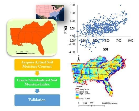
2. Materials and Methods

2.1. Data Acquisition

We used the Level 3 soil moisture data from L-Band Radiometer (SMAP L3_SM_P) on board the NASA satellite Soil Moisture Active Passive (SMAP). The SMAP Level 3 product is a daily global radiometer-only soil moisture product, which provides direct soil moisture measurement at 6 AM local solar time in the top 5-cm layer of the soil column in units of m3/m3 [27]. We obtained the data from NASA’s Earth Observing System Data and Information System (EOSDIS) Reverb Echo portal on EARTHDATA, and requested to transform NetCDF files into GeoTIFFs with the WGS 1984 Geographic Coordinate System.
The second dataset is the soil moisture data from NASA NLDAS. The NLDAS Noah Land Surface Model (LSM) L4 Hourly 0.125 × 0.125 degree V002 data that measure the top 10-cm soil moisture were downloaded from Goddard Earth Sciences (GES) Data and Information Center data portal, Mirador [28]. The NLDAS data time zone was Coordinated Universal Time (UTC), which has an overall six-hour time difference compared with the SMAP local solar time. Therefore, 1200 UTC data were collected for each day over the 36 years.
The third dataset is from the Soil Climate Analysis Network (SCAN). SCAN stations use probes to collect soil moisture data across the United States [29]. The probes were dielectric constant measuring devices placed at 5.08 cm depth [29]. The USDA National Resources Conservation Service (NRCS) provides the SCAN dataset as downloadable .csv tables. Table 1 shows the parameters and the uses of the data.

2.2. Data Processing

SMAP reached its orbit in January 2015, and the data were available since 1 April 2015. Therefore, only less than two years of data have been recorded at the time of this study. A pre-processing of the SMAP data removed invalid values and outliers. The units of SMAP and NLDAS soil moisture do not match. SMAP measures volume of water per unit volume of soil. NLDAS measures soil moisture in units of kilogram per square meter of soil over variable thicknesses. Equation (1) converts the unit of NLDAS to the volume ratio that is similar to SMAP units.
SM NLDAS   ( kg / m 2 ) W × T
where SMNLDAS represents the original soil moisture value and W is the density of water, or 1000 kilograms per cubic meter. T is the thickness of soil measured by NLDAS; in this case T is 0.1 m because NLDAS measures top 10-cm soil moisture.
We also notice the inconsistency of the soil depth measured by NLDAS and SMAP. The NLDAS measures the top 10 cm of the soil, 5 cm deeper than that of SMAP. Even though, according to Velpuri et al., SMAP shows a strong relationship with most soil moisture measurements at less than 20 cm depth [30]. We used a linear transformation to calibrate the two datasets. An example of the calibration on the NLDAS data is in Appendix A. Table A1 lists the calibration coefficients between NLDAS and SMAP.

2.3. Data Analysis

For each Julian day, there are 36 NLDAS observations from the past 36 years. Therefore, we were able to calculate the mean ( μ N L D A S ) and standard deviation ( σ N L D A S ) of each day. The daily SSI was calculated with Equation (2):
S S I = x SMAP μ N L D A S σ N L D A S
where xSMAP is the soil moisture content from SMAP Level 3 data for a single day, μNLDAS is the mean value of soil moisture content for the corresponding day from NLDAS, and σNLDAS is the standard deviation.

2.4. Validation

The SMAP mission specifies the accuracy of soil moisture to be within 0.04 (4%) m3/m3 volumetric in low or moderately vegetated areas in the following conditions [31]:
  • Vegetation water content ≤ 5 kg/m2
  • Urban fraction ≤ 0.25
  • Water fraction ≤ 0.1
  • Digital Elevation Model (DEM) slope standard deviation ≤ 3 degrees
Unfortunately, the southeast United States is not in the area where those accuracies are coherent. Therefore, we need to use other data sources to validate the soil moisture product. The validation was performed by comparing the soil moisture daily data from SMAP and NLDAS to daily soil moisture data retrieved from USDA SCAN stations. Table 2 lists the selected seven SCAN stations across the southeastern U.S. We selected the stations with a long-term collection of data, located in agricultural lands, plains, or grasslands, and reprehensive of diverse weather conditions. The comparison between SMAP and SCAN was on a daily basis, from 31 March 2015 to 16 July 2016. We also compared SCAN data and NLDAS data for 12 months, starting in January 2015 and ending in December 2015.
SSI was validated by several soil moisture products, including PDSI and MODIS data. PDSI data for April 2015 were downloaded as NetCDF files in the WGS 1984 Geographic Coordinate System from the National Integrated Drought Information System on the U.S. Drought Portal. We derived a normalized difference water index (NDWI) from MODIS surface reflectance data [11,32,33]:
NDWI = NIR SWIR NIR + SWIR
where NIR is the near infrared reflectance and SWIR is the short-wave infrared reflectance of the MODIS data. Both PDSI and NDWI data were resampled to 36 km for the SSI validation.

3. Results

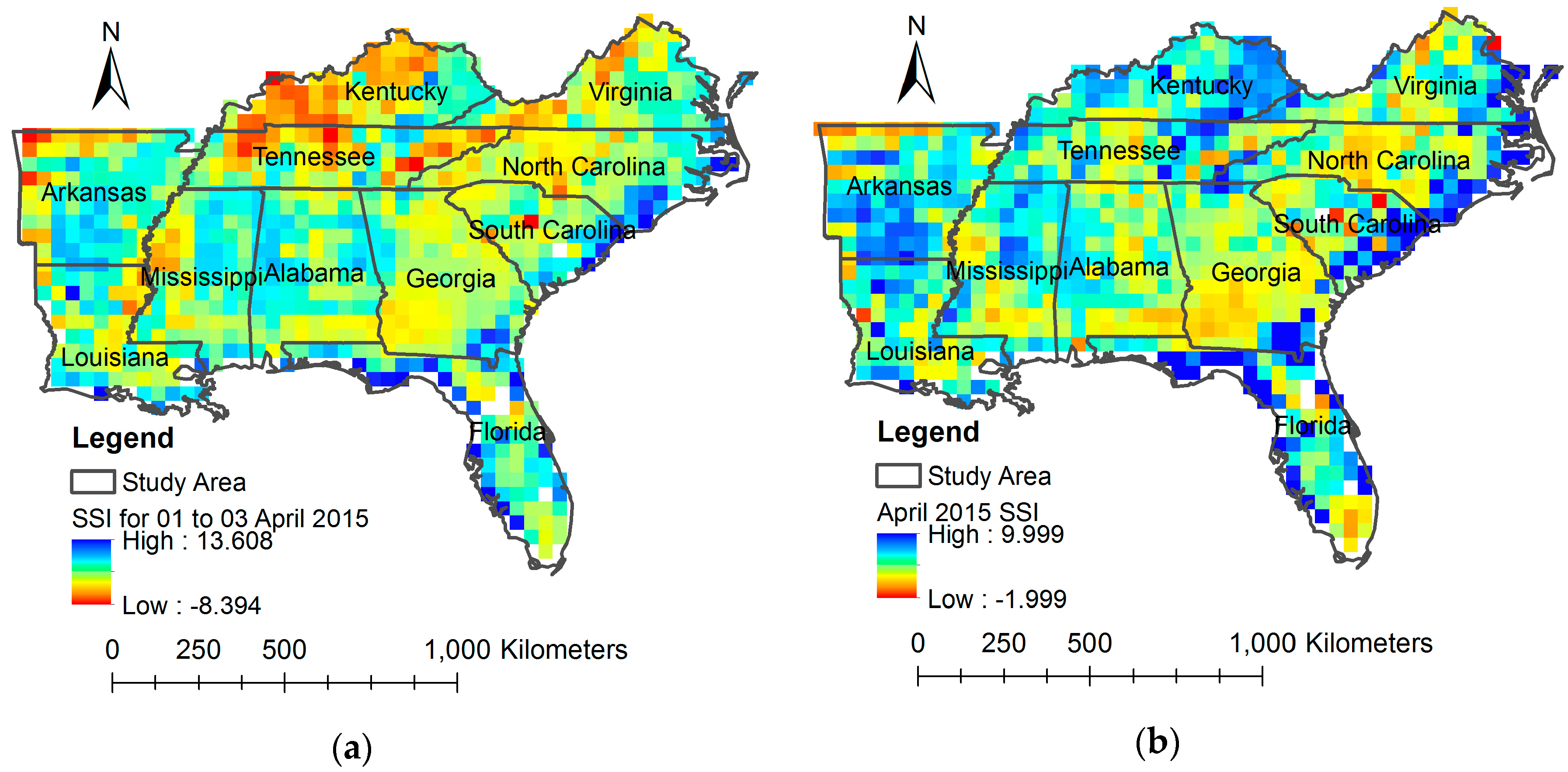
3.1. SSI Spatial Analysis

The first SMAP record was on 1 April 2015, when the SMAP radiometer started collecting routine science data. As SMAP requires a minimum of three consecutive days to cover the globe, the SSI results for each of the three consecutive days were mosaicked to cover the study area (Figure 1a). The standardized SSI is a z-score, indicating how many standard deviations that a SMAP value is from the historic mean. The yellow to red colors indicate negative z-scores, which means the values are lower than the historic soil moisture mean for those pixels. The green to blue colors indicate positive z-scores, which means the values are higher than the historic soil moisture average for those pixels.
Figure 1a reveals the regional climate variability for 1 to 3 April 2015 in the southeastern United States. Along the southeast coastal area ranging from North Carolina to Florid, the soil moisture values were significantly above their historic means. This pattern diminishes as the distance off the coast increased. The high SSI values in the southern North Carolina and western Florida indicated a wet soil condition compared to the past 36 years. On the contrary, the western Virginia and eastern Tennessee observed a below-average SSI, which indicated a dry soil condition compared to the past 36 years. Western Kentucky and Northwestern Tennessee observed severe dry soil conditions. The remaining states, including Louisiana, Mississippi, Alabama, and most of Arkansas, Georgia, and part of Virginia, North Carolina, and South Carolina were in an average condition. Arkansas and western Louisiana generally observed average soil moisture, with several lower values along the western border, and one pixel of higher value in northwestern Louisiana. SSI for April 2015, in contrast, shows the soil is generally wetter, except southern Mississippi, southern Alabama, Georgia, North Carolina and southern Florida (Figure 1b).

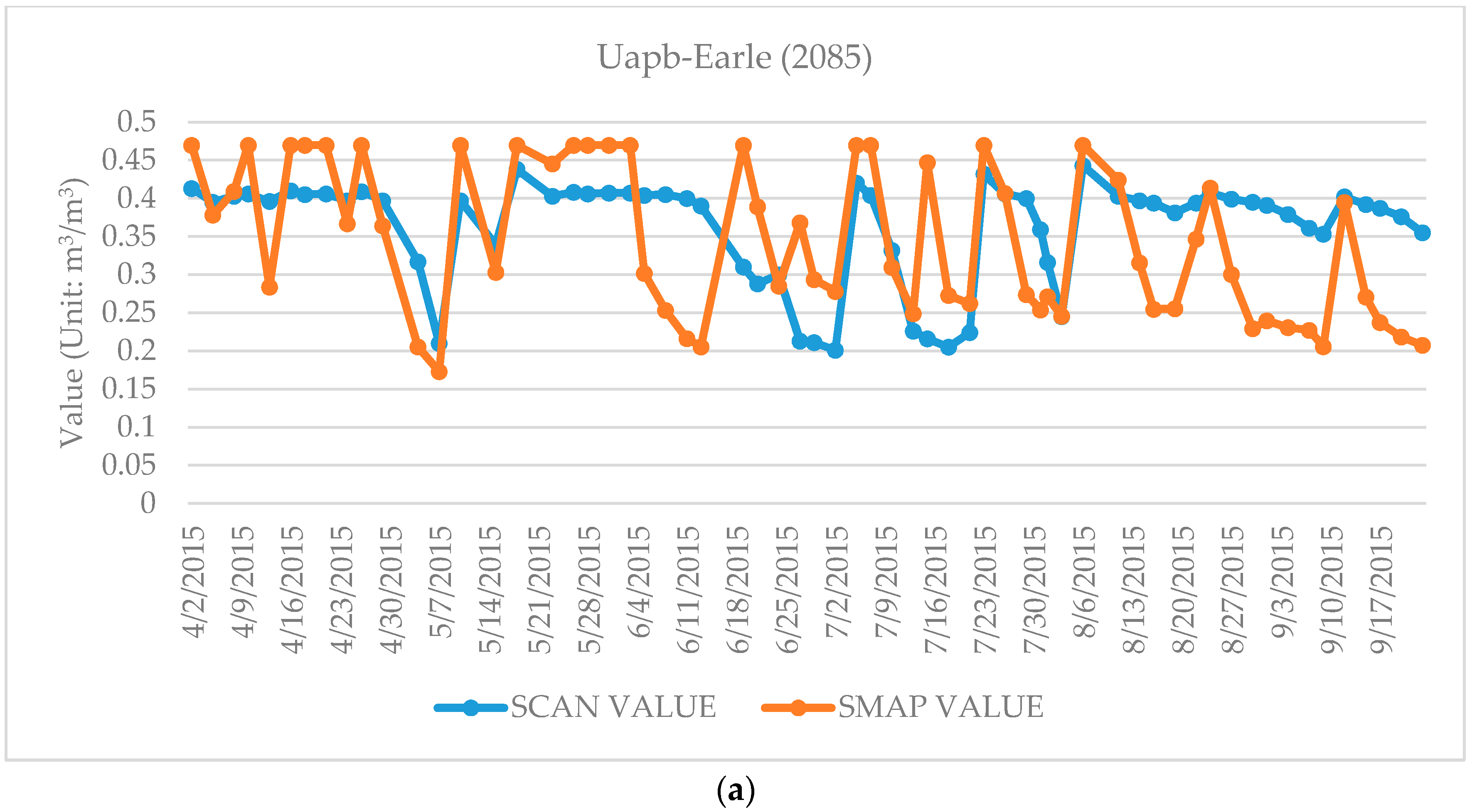
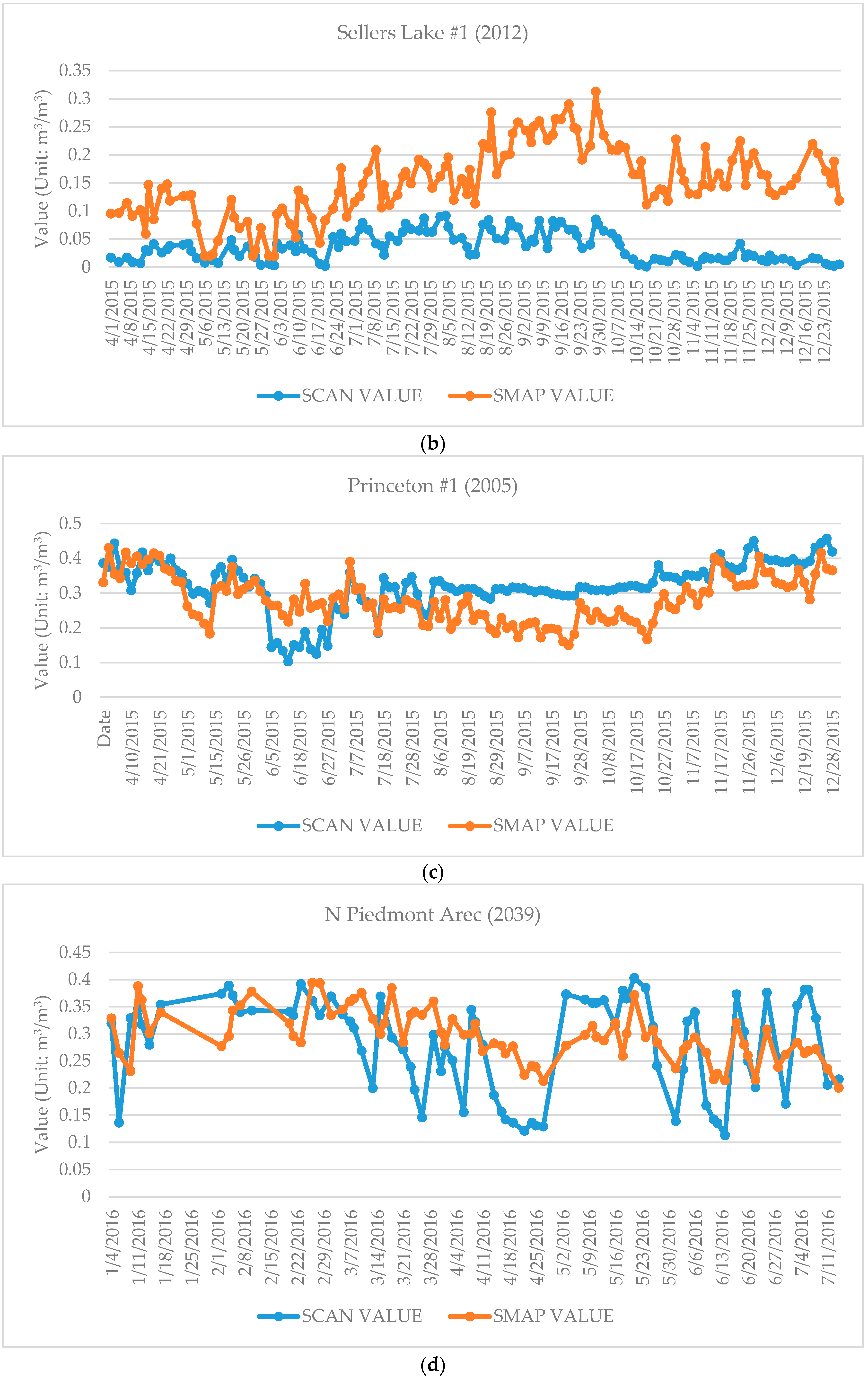
3.2. Validation Result

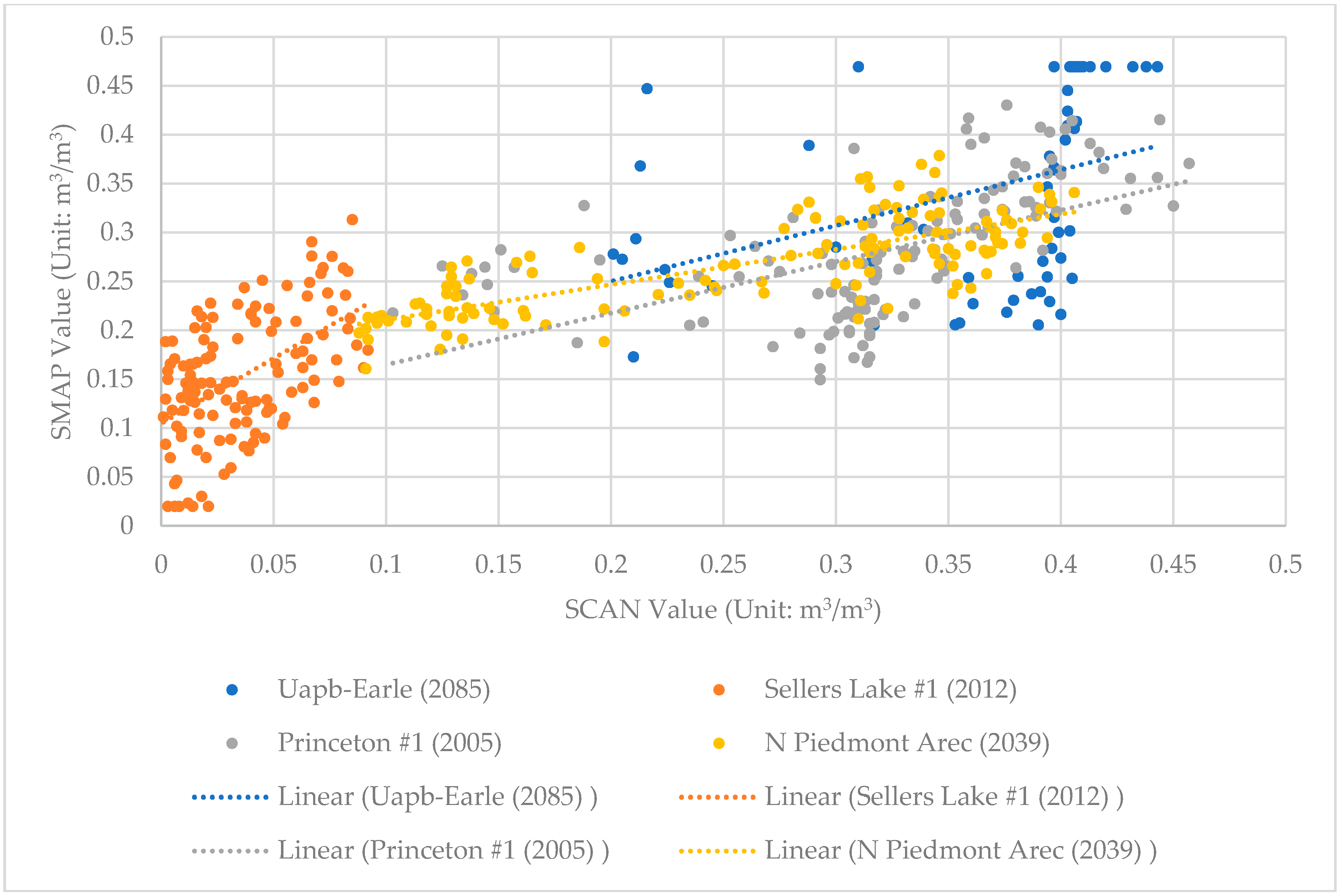
3.2.1. SMAP Validation

The correlations between SMAP soil moisture data and the SCAN data were between 0.1506 and 0.9177. The correlations between SCAN and NLDAS data were between 0.376 and 0.7742. The RMSEs for SMAP were between 0.0428 and 0.1379, which do not meet SMAP mission’s specification (0.04 or 4% m3/m3) for low or moderately vegetated areas. Given that the southeast United States are mostly covered by high vegetation, the validation result is still acceptable for drought monitoring. Table 3 shows the R-squared and RMSE for SMAP in 2015 and 2016. Note that the correlation for station Uapb-Earle in 2016 was invalid due to missing SCAN data.

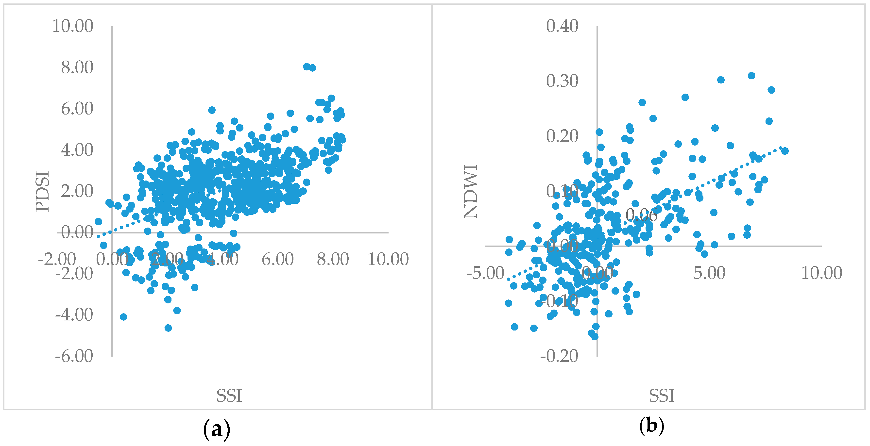
3.2.2. Validation with PDSI and NDWI

PDSI is a standardized index that spans −10 (dry) to +10 (wet) [34]. Figure 2a shows the reference image of PDSI for April 2015. Compare to the SSI result for April 2015 (Figure 1b), the drought patterns are generally consistent. The scatter plot shows the correlation between SSI and PDSI is moderate: the correlation coefficient (r) was 0.52 (Figure 3a). PDSI is effective in determining long-term drought [34], but not for short time periods such as daily soil moisture deficiency. For daily comparison, MODIS NDWI was used to test the accuracy of short-term SSI.
NDWI is dimensionless and ranges between −1 (low vegetation water content) to +1 (high vegetation water content) [33]. Figure 2b shows that the NDWI calculated for 1 to 3 April 2015 has a quite different pattern from the PDSI for April 2015 (Figure 2a), but has a very similar spatial pattern compared with the SSI for 1 to 3 April 2015 (Figure 1a). The dry condition monitored through NDWI in western Kentucky and western Tennessee matches the low-value areas by SSI. The wet condition in Florida from NDWI was also observed from SSI. This suggests that SSI is more sensitive than PDSI for short-term drought monitoring. Scatter plot shows the correlation between SSI and NDWI is strong: the correlation coefficient (r) value was 0.56 (Figure 3b).

4. Discussion

The SMAP validation revealed that the average correlation between SMAP data and SCAN data were 0.4611 for 2015 and 0.6240 for 2016. Four low R-squared values suggested some discrepancy between SMAP and SCAN data. The R-squared at the Uapb-Earle station in Arkansas for the year 2015 was exceptionally low (0.1506). Low R-squared values were also found at the N Piedmont Arec station in Virginia (for 2016), the Sellers Lake #1 station in Florida (for 2015), and the Princeton #1 station in Kentucky (for 2015). Figure 4 shows the correlations between SCAN values and SMAP values for the four stations.
To discover what caused these significantly low accuracies in the abovementioned stations, we created time-series plots to identify the outliers between SMAP and SCAN (Figure 5).
Figure 5a shows that at the Uapb-Earle station, the SMAP data and SCAN data are generally correlated, but the correlation drastically changed from around 4 June to 25 June, and then from 13 August to 10 September. Figure 5b shows the large disagreement at the Sellers Lake station. SCAN soil moisture values remained below 0.1 while SMAP abruptly jumped above 0.25 from August 21 to September 30. Figure 5c shows that at Princeton station, the agreement between SMAP and SCAN was good from April 2015 to May. Nevertheless, this harmony was broken on 5 June until 27 June. In these days, SCAN observations were between 0.1 and 0.2, while SMAP data were between 0.2 to 0.3. From 6 August to 15 November, SMAP data were consistently lower than the SCAN data. Figure 5d shows that at N Piedmont Arec station there was a reverse trend between SMAP and SCAN from 18 January to 1 February, then 5 March to 18 March, and then from 8 April to 14 April. One of the major limitations of using SCAN data for satellite data validation is that the scales are different. The station observations are from precise sensors buried in soil, which only see a few inches of soil volume, while satellite sensors collect surface radiance from a large footprint (e.g., SMAP ~ 36 × 36 km) [15]. The satellite data are complex averages of the surface conditions and environments. Therefore, although direct comparison between the two datasets has been a common approach, it may not offer sufficient accuracy assessment of the satellite data.
Another limitation is the high SSI scores along the coastal areas in Figure 1. It has been reported in the literature that open water might lead to considerably biased soil moisture retrievals [35]. Make corrections of the coastal soil moisture data would require huge amount of efforts and additional data, including detailed land cover data and in-situ observations at much finer resolutions.
The last limitation of the SSI is that the calculation was based on the normality assumption of the historical data. The outliers (droughts) detected by the deviation from means are only valid if the assumption holds. Therefore, this approach is sensitive to data noise. Although we used 36 years of data to calculate the means and standard deviations, the SSI model will benefit from including longer periods if possible.

5. Conclusions

This research proposes a climate index called the standardized soil moisture index (SSI) to detect droughts. SSI was derived from satellite soil moisture data of SMAP and the long-term land surface model NLDAS data to facilitate drought detection in short terms such as three days. By doing so, drought warnings can reach the farmers and foresters at a timely fashion.
We first validated the accuracies of the input data. The SMAP soil moisture data displayed good statistical correlations (R2 = 0.4611 for 2015 and 0.6240 for 2016) with in-situ SCAN data and with acceptable RMSEs (0.0819 for 2015 and 0.0748 for 2016). However, we found large inconsistency in areas that are not friendly for satellite observations such as vegetation, water bodies, urban, and high slope terrains.
The validation of SSI through PDSI and NDWI suggested SSI was an effective measure of soil moisture conditions. The correlation between SSI and PDSI for April 2015 is acceptable (r = 0.52), and the correlation between SSI and NDWI is slightly better (r = 0.56). PDSI is a monthly index. Therefore, SSI could provide shorter-term warnings than PDSI. Thus, SSI is a favorable index over PDSI for drought detection.
In summary, our SSI is a new climate index for drought detection. It is computed from daily satellite data and statistics from long-term soil moisture data, and therefore can provide short-term warning of drought conditions. Moreover, SSI is easy to interpret for farmers and foresters due to its simple and transparent statistical construct. Our research validated the SSI using multiple external sources of soil moisture data. The inconsistency of satellite observations with ground data could be solved by downscaling satellite data in the future work.

Supplementary Materials

The following are available online at https://0-www-mdpi-com.brum.beds.ac.uk/2072-4292/10/2/301/s1, Video: Southeast U.S. Agriculture-NASA DEVELOP Summer 2016 @ Wise County.

Acknowledgments

This material is based upon work supported by NASA through contract NNL11AA00B and cooperative agreement NNX14AB60A. We would like to thank DeWayne Cecil, Michael Bender, Michael Brooke, and Bob VanGundy for their help on this project. Thank Yousra Benchekroun, and Grant Bloomer for their help with the data and material processing. Thank Robert Rohli for the help with experimental design and paper revision.

Author Contributions

Yaping Xu and Kenton W. Ross conceived and designed the experiments; Yaping Xu and Kimberly Berry processed the data; Cuiling Liu and Yaping Xu analyzed the data and made the maps; Yaping Xu and Lei Wang wrote the paper; Lei Wang and Kimberly Berry revised the paper.

Conflicts of Interest

The authors declare no conflict of interest. The founding sponsors had no role in the design of the study; in the collection, analyses, or interpretation of data; in the writing of the manuscript, and in the decision to publish the results.

Appendix A

The calibration of NLDAS data for calculation SSI.
Table A1 shows the statistic information obtained from ArcGIS.
Take April 01, 2015 as an example,
  • Mean (NLDAS) = 23.705
  • STD (NLDAS) = 5.5943
  • Mean (SMAP) = 0.35731
  • STD (SMAP) = 0.11158
Therefore,
  • Mean (NLDAS) = 66.343 × Mean(SMAP)
  • STD (NLDAS) = 50.137 × STD(SMAP)
in which NLDAS Value = 100 times of SMAP Value because of the unit difference.
Therefore, in the equation of SSI, we should divide the mean of NLDAS by 66.343, and divide the STD by 50.137 to get a predicted SMAP value.
Table A1. NLDAS calibration.
DateNLDAS MeanSMAP MeanN/SNLDAS StdSMAP StdN/S
1 April 201523.7050.3573166.345.59430.1115850.13
2 April 201523.4130.3573465.525.71490.0867165.91
3 April 201523.9120.4032259.306.66330.0915372.80
1 April 201626.8600.3817170.376.50420.0834677.93
2 April 201626.0870.4433158.845.40960.0734673.64
3 April 201624.7920.4102160.445.40990.0888760.88
1 April 201723.8290.3631565.626.60620.1041663.43
2 April 201723.036N/A1N/A 16.4982N/A 1N/A 1
3 April 201725.4420.3616170.368.34950.1241267.27
1 2 April 2017 calibration was not available due to the missing data for SMAP.

References

  1. Melillo, J.M.; Richmond, T.; Yohe, G. Climate Change Impacts in the United States; Government Printing Office: Washington, DC, USA, 2014.
  2. McNulty, S.; Director, S.H.; Wiener, S.; Treasure, S.H.; Myers, J.M.; Farahani, H.; Fouladbash, L.; Marshall, D.; Steele, R.F. Southeast regional climate hub assessment of climate change vulnerability and adaptation and mitigation strategies. Agric. Res. Serv. 2015, 2015, 1–61. [Google Scholar]
  3. Parry, M.; Canziani, O.F.; Palutikof, J.P.; van der Linden, P.J.; Hanson, C.E. Climate Change 2007: Impacts, Adaptation and Vulnerability; Cambridge University Press: Cambridge, UK, 2007; Volume 4. [Google Scholar]
  4. Intergovernmental Panel on Climate Change. Climate Change 2014—Impacts, Adaptation and Vulnerability: Regional Aspects; Cambridge University Press: Cambridge, UK, 2014. [Google Scholar]
  5. Field, C.B. Managing the Risks of Extreme Events and Disasters to Advance Climate Change Adaptation: Special Report of the Intergovernmental Panel on Climate Change; Cambridge University Press: Cambridge, UK, 2012. [Google Scholar]
  6. SERCH LIGHTS Alerts Help Land Managers Prepare for Drought. Available online: https://forestthreats.org/research/projects/2015-accomplishment-highlights/serch-lights-alerts-help-land-managers-prepare-for-drought/ (accessed on 1 August 2016).
  7. Fact Sheet: Drought. Available online: http://www.nws.noaa.gov/om/csd/graphics/content/outreach/brochures/FactSheet_Drought.pdf (accessed on 1 August 2016).
  8. Thornthwaite, C.W.; Mather, J. The Water Balance; Drexel Institute Of Technology-Laboratory of Climatology: Centerton, NJ, USA, 1955. [Google Scholar]
  9. Ritchie, J. Soil water balance and plant water stress. In Understanding Options for Agricultural Production; Springer: Berlin, Germany, 1998; pp. 41–54. [Google Scholar]
  10. Palmer, W.C. Meteorological Drought; US Department of Commerce Weather Bureau: Washington, DC, USA, 1965; Volume 30.
  11. Zargar, A.; Sadiq, R.; Naser, B.; Khan, F.I. A review of drought indices. Environ. Rev. 2011, 19, 333–349. [Google Scholar] [CrossRef]
  12. Sivakumar, M.; Motha, R.; Wilhite, D.; Wood, D. Agricultural Drought Indices Proceedings of an Expert Meeting. 2–4 June 2010, Murcia, Spain; World Meteorological Organization: Geneva, Switzerland, 2010. [Google Scholar]
  13. Sheikh, V.; Visser, S.; Stroosnijder, L. A simple model to predict soil moisture: Bridging event and continuous hydrological (BEACH) modelling. Environ. Model. Softw. 2009, 24, 542–556. [Google Scholar] [CrossRef]
  14. Meng, L.; Quiring, S.M. A comparison of soil moisture models using soil climate analysis network observations. J. Hydrometeorol. 2008, 9, 641–659. [Google Scholar] [CrossRef]
  15. Crow, W.T.; Berg, A.A.; Cosh, M.H.; Loew, A.; Mohanty, B.P.; Panciera, R.; Rosnay, P.; Ryu, D.; Walker, J.P. Upscaling sparse ground—Based soil moisture observations for the validation of coarse-resolution satellite soil moisture products. Rev. Geophys. 2012, 50. [Google Scholar] [CrossRef]
  16. De Rosnay, P.; Drusch, M.; Boone, A.; Balsamo, G.; Decharme, B.; Harris, P.; Kerr, Y.; Pellarin, T.; Polcher, J.; Wigneron, J.P. Amma Land Surface Model Intercomparison Experiment coupled to The Community Microwave Emission Model: Almip-Mem. J. Geophys. Res. 2009, 114. [Google Scholar] [CrossRef]
  17. Petropoulos, G.P.; Ireland, G.; Barrett, B. Surface soil moisture retrievals from remote sensing: Current status, products & future trends. Phys. Chem. Earth 2015, 83, 36–56. [Google Scholar]
  18. Keyantash, J.; Dracup, J.A. The quantification of drought: An evaluation of drought indices. Bull. Am. Meteorol. Soc. 2002, 83, 1167–1180. [Google Scholar] [CrossRef]
  19. Hayes, M.J. Drought Indices; Wiley: Hoboken, NJ, USA, 2006. [Google Scholar]
  20. Quiring, S.M.; Papakryiakou, T.N. An evaluation of agricultural drought indices for the Canadian prairies. Agric. For. Meteorol. 2003, 118, 49–62. [Google Scholar] [CrossRef]
  21. McKee, T.B.; Doesken, N.J.; Kleist, J. The relationship of drought frequency and duration to time scales. In Proceedings of the 8th Conference on Applied Climatology, Anaheim, CA, USA, 17–22 January 1993; American Meteorological Society: Boston, MA, USA, 1993; pp. 179–183. [Google Scholar]
  22. Edwards, D.; McKee, T. Characteristics of 20th Century Drought in the United States at Multiple Time Scales; Colorado State University, Department of Atmospheric Science: Fort Collins, CO, USA, 1997. [Google Scholar]
  23. Illston, B.G.; Basara, J.B.; Crawford, K.C. Seasonal to interannual variations of soil moisture measured in Oklahoma. Int. J. Climatol. 2004, 24, 1883–1896. [Google Scholar] [CrossRef]
  24. What Is the U.S. Drought Monitor? Available online: http://droughtmonitor.unl.edu/data/docs/USDMbrochure.pdf (accessed on 19 November 2016).
  25. Al-Yaari, A.; Wigneron, J.P.; Kerr, Y.; Rodriguez-Fernandez, N.; O’Neill, P.E.; Jackson, T.J.; De Lannoy, G.J.M.; Al Bitar, A.; Mialon, A.; Richaume, P.; et al. Evaluating soil moisture retrievals from ESA’s SMOS and NASA’s SMAP brightness temperature datasets. Remote Sens. Environ. 2017, 193, 257–273. [Google Scholar] [CrossRef]
  26. Xia, Y.; Sheffield, J.; Ek, M.B.; Dong, J.; Chaney, N.; Wei, H.; Meng, J.; Wood, E.F. Evaluation of multi-model simulated soil moisture in NLDAS-2. J. Hydrol. 2014, 512, 107–125. [Google Scholar] [CrossRef]
  27. National Aeronautics and Space Administration (NASA). SMAP handbook. In Mapping Soil Moisture and Freeze/Thaw from Space; Jet Propulsion Laboratory: Pasadena, CA, USA, 2014. [Google Scholar]
  28. Xia, Y.; Ek, M.B.; Wu, Y.; Ford, T.; Quiring, S.M. Comparison of NLDAS-2 simulated and NASMD observed daily soil moisture. Part I: Comparison and analysis. J. Hydrometeorol. 2015, 16, 1962–1980. [Google Scholar] [CrossRef]
  29. Soil Climate Analysis Network (SCAN). Brochure. Available online: https://www.wcc.nrcs.usda.gov/scan/SCAN_brochure.pdf (accessed on 1 August 2016).
  30. Velpuri, N.M.; Senay, G.B.; Morisette, J.T. Evaluating new SMAP soil moisture for drought monitoring in the rangelands of the us high plains. Rangelands 2016, 38, 183–190. [Google Scholar] [CrossRef]
  31. Colliander, A.; Jackson, T.; Bindlish, R.; Chan, S.; Das, N.; Kim, S.; Cosh, M.; Dunbar, R.; Dang, L.; Pashaian, L. Validation of SMAP surface soil moisture products with core validation sites. Remote Sens. Environ. 2017, 191, 215–231. [Google Scholar] [CrossRef]
  32. McFeeters, S.K. The use of the Normalized Difference Water Index (NDWI) in the delineation of open water features. Int. J. Remote Sens. 1996, 17, 1425–1432. [Google Scholar] [CrossRef]
  33. Gao, B.-C. Ndwi—A Normalized Difference Water Index for remote sensing of vegetation liquid water from space. Remote Sens. Environ. 1996, 58, 257–266. [Google Scholar] [CrossRef]
  34. Dai, A.; Trenberth, K.E.; Qian, T. A global dataset of palmer drought severity index for 1870–2002: Relationship with soil moisture and effects of surface warming. J. Hydrometeorol. 2004, 5, 1117–1130. [Google Scholar] [CrossRef]
  35. Wu, Q.; Liu, H.; Wang, L.; Deng, C. Evaluation of AMSR2 soil moisture products over the contiguous United States using in situ data from the International Soil Moisture Network. Int. J. Appl. Earth Obs. Geoinf. 2016, 45, 187–199. [Google Scholar] [CrossRef]
Figure 1. (a) Mosaic of the three consecutive standardized soil moisture index (SSI) maps from 1 to 3 April 2015. Areas in yellow to red represent areas that are experiencing very dry conditions, indicating drought. (b) SSI map for the whole month of April 2015.
Remotesensing 10 00301 g001
Figure 2. (a) Palmer drought severity index (PDSI) for April 2015. Areas in yellow and red represent areas that are experiencing dry conditions; (b) Normalized difference water index (NDWI) calculated for 01 to 03 April 2015. Likewise, areas in yellow and red represent areas that are experiencing low vegetation water content and therefore a dry condition.
Remotesensing 10 00301 g002
Figure 3. (a) Scatter plot for April 2015. The correlation between SSI and PDSI is moderate (r = 0.52); (b) Scatter plot for 1 to 3 April 2015. The correlation between SSI and NDWI is strong (r = 0.56).
Remotesensing 10 00301 g003
Figure 4. Scatter plot between SCAN values and SMAP values for the four anomaly stations with the R-squared values: Uapb-Earle station in Arkansas (for the year 2015), R-squared value was 0.1506; N Piedmont Arec station in Virginia (for 2016), R-square value was 0.2499; the Sellers Lake #1 station in Florida (for 2015), R-square value was 0.2827; and the Princeton #1 station in Kentucky (for 2015), R-square value was 0.3115.
Remotesensing 10 00301 g004
Figure 5. SMAP and SCAN time plot comparison to identify the anomaly: (a) Uapb-Earle station in Arkansas (2085); (b) Sellers Lake #1 station in Florida (2012); (c) Princeton #1 station in Kentucky (2005); and (d) N Piedmont Arec station in Virginia (2039).
Remotesensing 10 00301 g005aRemotesensing 10 00301 g005b
Table 1. Data description.
Platform & SensorParameterUse
SMAP
Passive Radiometer
Soil moisture, Level-3, 36 km resolutionDaily measurement of soil moisture
NLDAS Soil moisture, Noah modelHistorical mean and standard deviation of soil moisture
USDA SCAN Soil moistureValidation
Table 2. Soil Climate Analysis Network (SCAN) stations used for validation.
Station IDState CodeStation Name
2013GAWatkinsville #1
2024MSGoodwin Ck Pasture
2053ALWtars
2039VAN Piedmont Arec
2005KYPrinceton #1
2012FLSellers Lake #1
2085ARUapb-Earle
Table 3. Soil Moisture Active Passive (SMAP) validation with SCAN stations.
Station IDStation NameR2 for 2015R2 for 2016RMSE for 2015RMSE for 2016
2013Watkinsville #10.68020.91240.05670.0791
2024Goodwin Ck Pasture0.76340.68170.07950.0591
2053Wtars0.46120.91770.06240.0428
2039N Piedmont Arec0.57830.24990.07120.0774
2005Princeton #10.31150.51440.07620.0526
2012Sellers Lake #10.28270.4680.12880.1379
2085Uapb-Earle0.1506N/A0.0983N/A
Average 0.46110.62400.08190.0748

