Classification and Mapping of Paddy Rice by Combining Landsat and SAR Time Series Data

Abstract

Rice is an important food resource, and the demand for rice has increased as population has expanded. Therefore, accurate paddy rice classification and monitoring are necessary to identify and forecast rice production. Satellite data have been often used to produce paddy rice maps with more frequent update cycle (e.g., every year) than field surveys. Many satellite data, including both optical and SAR sensor data (e.g., Landsat, MODIS, and ALOS PALSAR), have been employed to classify paddy rice. In the present study, time series data from Landsat, RADARSAT-1, and ALOS PALSAR satellite sensors were synergistically used to classify paddy rice through machine learning approaches over two different climate regions (sites A and B). Six schemes considering the composition of various combinations of input data by sensor and collection date were evaluated. Scheme 6 that fused optical and SAR sensor time series data at the decision level yielded the highest accuracy (98.67% for site A and 93.87% for site B). Performance of paddy rice classification was better in site A than site B, which consists of heterogeneous land cover and has low data availability due to a high cloud cover rate. This study also proposed Paddy Rice Mapping Index (PMI) considering spectral and phenological characteristics of paddy rice. PMI represented well the spatial distribution of paddy rice in both regions. Google Earth Engine was adopted to produce paddy rice maps over larger areas using the proposed PMI-based approach.

1. Introduction

Rice is one of the important food resources for most of the world’s population, especially those in Asia [1,2]. The annual average of rice consumption per capita was approximately 54 kg during 2017–2018 (Agricultural Market Information System (AMIS), http://statistics.amis-outlook.org/), and the consumption has increased with increasing world population [3]. Muthayya et al. [4] noted that the demand for rice over the next 30 years is expected to increase by 90% in Asia. Paddy rice mapping and monitoring are crucial for food security and agricultural mitigation because they allow for identifying and forecasting rice production [5]. In general, the annual or seasonal surveys have been conducted for measuring cultivated areas during the crop growing season [5,6]. The sampling survey, however, is costly, labor-intensive, and time-consuming. In addition, the survey based paddy rice mapping has a relatively slow update cycle (e.g., every five years). Rice cultivated areas often change due to human activities as well as natural disasters such as drought, floods, and wildfire. Thus, up-to-date information on paddy rice areas is essential for decision makers, scientists, and also farmers to monitor and manage the areas in a timely and sustainable manner.

Satellite remote sensing has been employed as an alternative with advantages of high temporal resolution and spatial continuity. There are several studies for paddy rice classification using single optical sensor data, such as Moderate Resolution Imaging Spectroradiometer (MODIS) and Advanced Very High Resolution Radiometer (AVHRR) [7,8]. However, mixed pixels have often caused misclassification when using single sensor data (e.g., MODIS) [9]. Multi-temporal and high-resolution data have been used to overcome such a mixed pixel problem [10]. Recent studies have emphasized the capability of multi-temporal data to identify paddy rice areas because paddy rice has its own phenology (e.g., transplanting), which is a distinct characteristic of paddy rice compared to other crop or land cover types [11,12,13,14,15,16,17]. Clauss et al. [18] mapped paddy rice in China using Support Vector Machine (SVM) with MODIS time series data. Their approach performed well to map paddy rice with an overall accuracy of 90%. Jin et al. [9] attempted to map paddy rice distribution using multi-temporal Landsat data at regional scale with phenology information. They used a rule-based decision tree approach to determine optimal threshold values to map paddy rice using multi-temporal Normalized Difference Vegetation Index (NDVI), Enhanced Vegetation Index (EVI), and Land Surface Water Index (LSWI) as input data. The results showed the coefficient of determination (R²) of 0.85 between satellite-based and census recorded paddy rice areas. Dong et al. [19] developed a time series Landsat-based paddy rice mapping platform to produce paddy rice maps from 1986 to 2010. Vegetation indices were used to conduct paddy rice mapping with a five-year interval based on a land cover-adapted thresholding approach.

Although optical sensor data are useful to map paddy rice, there is a limitation for data acquisition due to cloud contamination. Synthetic Aperture Radar (SAR) data have been used to complement the cloud problems of optical sensor images because SAR data are not influenced by weather conditions [20,21]. Several studies employed SAR data for land cover/land use as well as paddy rice mapping [1,21,22,23,24]. Optical sensor and SAR data have complementary information. Multi- or hyperspectral data provide information of reflective and emissive features of the Earth’s surface, while the SAR data provide information about the surface roughness, texture and dielectric properties of natural and man-made objects [22,25]. Thus, the integration of multispectral and SAR data produces more reliable results than those from single sensor data [25]. Over the years, research efforts have been made in fusion of different sensor data in the remote sensing field [1,23,26,27]. Torbick et al. [26] aimed to monitor paddy rice agriculture fusing optical vegetation indices from Landsat 8 and dual-polarization C and L band backscattering coefficients from Sentnel-1 and PALSAR-2 across the Myanmar using a random forest (RF) approach. The results showed the accuracy with R² of 0.78 for the harvested rice areas in comparison with census statistics. They concluded that the fusion of optical and SAR data has a great potential to monitor and analyze paddy rice production.

Given the increasing interests in remote sensing-based paddy rice mapping and monitoring, several review papers on this topic have been published [5,17,28]. Dong et al. [17] divided paddy rice mapping studies into four categories, using (1) reflectance data and statistical approaches, (2) vegetation index (VI) and enhanced statistical approaches, (3) temporal analysis approaches with VI or RADAR data, and (4) phenology-based approaches. They discussed the current challenges and opportunities in future paddy rice mapping: to improve algorithms with the development of land cover classification approaches, to improve data acquisition capacity with high spatial resolution (~30 m) such as combined Landsat and Sentinel-2 data, and to improve computing capacity such as using Google Earth Engine. In particular, the Landsat series have been provided for free with an opening from the archive datasets to the general public. Added to this benefit are large swaths with a width of 185-km and a 16-day temporal resolution, which produces valuable information for the repeated measurement of space and time [29,30]. Moreover, accumulated archives with more than 40 years of data have the potential to fuel long-term studies with regional and global land cover classifications [31]. Given this background, we identified some issues that should be improved. This present study investigated the following approaches to improve the identification of paddy rice areas over two distinct regions with different climatic and environmental characteristics:

• paddy rice classification using multi-sensor fusion (optical sensor and SAR) and multi-temporal data through machine learning approaches (RF and SVM);
• development of a paddy rice mapping index (PMI) while considering spectral and phenological characteristics; and,
• paddy rice classification using Google Earth Engine based on the PMI approach over larger areas.

The present study aims at advance paddy rice classification by expanding the dimensionality of data on both spectral and temporal domains. We conducted paddy rice classification through fusion of optical sensor and SAR time series data using two machine learning approaches, RF and SVM. This study examined six schemes to identify the effect of data dimensionality on paddy rice classification. The six schemes composed of various combinations of input data by sensor and collection date considering the phenology of paddy rice over two different regions. This study also proposed Paddy rice Mapping Index (PMI) when considering the spectral and temporal characteristics of paddy rice that can be applied to areas that have different climatic and environmental characteristics.

2. Study Area and Data

2.1. Study Area

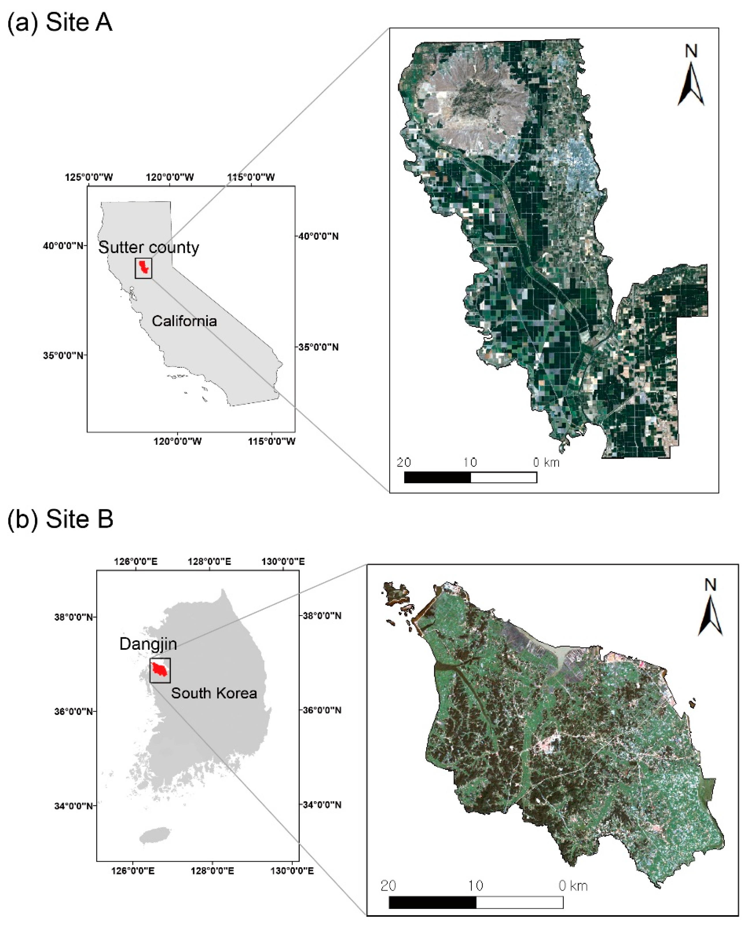
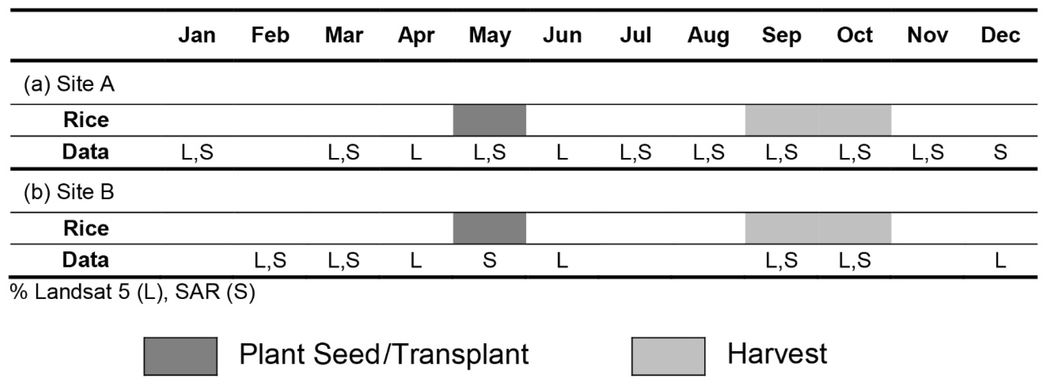
The study area consisted of two regions with different climatic and environmental characteristics (Figure 1). The first study site (site A) was Sutter County in California State, United States, which is known for its high rice productivity. About 90% of site A is composed of vegetated areas, and almost 40% of the vegetated areas are paddy rice. Temperature ranges from 4.06 °C in January to 36.11 °C in July on average, and the annual precipitation is around 558.8 mm. In site A, rice is planted mid-May by dropping rice seeds into flooded paddies from small planes (i.e., direct seeding) and harvested between September and October (Figure 2). The second study site (site B) was Dangjin in South Korea. Site B is one of the highest rice production regions in South Korea. Site B has relatively heterogeneous land covers, with many fragmented patches when compared to site A. The annual mean temperature is 11.4 °C and the annual precipitation is 1158.7 mm. Since South Korea has a rainy season between June and July caused by the Asian Monsoon, it is not easy to collect cloud-free satellite optical sensor images during this time. Rice planting and harvesting in site B occur at similar time intervals as site A (Figure 2). Unlike site A, manual or machine-based rice transplantation in May is common in site B.

2.2. Satellite Data

In this study, two types of time series satellite data (optical and SAR) were used. Multispectral Landsat 5, 7, and 8 level-1 images were acquired from the United States Geological Survey (USGS) (path/row 44/33 (for site A) and 116/34 (for site B)). Three visible bands, Blue (0.45–0.53 μm), Green (0.52–0.60 μm), and Red (0.63–0.69 μm), and three Infrared (IR) bands, near-infrared (NIR) (0.76–0.90 μm), shortwave-infrared 1 (SWIR1) (1.55–1.75 μm), and SWIR2 (2.08–2.35 μm), at 30 m spatial resolution were used. A total of 16 Landsat 5 images from 2007 to 2009 for site A, and 11 images from 2003 to 2005 at site B were acquired (

Table 1. Acquisition dates of satellite data at site A.

ALOS PALSAR	Landsat 5
29 December 2007	15 January 2009
	31 January 2009
26 March 2007	20 March 2009
28 March 2008	2 April 2008
	5 April 2009
	21 April 2009
13 May 2008	7 May 2009
	23 May 2009
	8 June 2009
	24 June 2009
1 July 2009	10 July 2009
	26 July 2009
13 August 2006	27 August 2009
26 September 2007	7 September 2007
1 October 2009	30 October 2009
13 November 2008	15 November 2009
27 December 2008

and

Table 2. Acquisition dates of satellite data at site B.

RADARSAT 1	Landsat 5
18 February 2004	12 February 2004
	13 March 2003
25 March 2005	18 March 2005
	29 March 2003
	31 March 2004
6 May 2003	30 April 2003
30 May 2003	1 June 2003
	3 June 2004
27 September 2003	21 September 2003
15 October 2004	9 October 2004
	12 December 2004

). Unlike site A, where enough cloud free images for every month are available, it is hard to obtain clear images at site B during the rainy season (June to July). Figure 2 shows data availability with crop schedules by month. Atmospheric correction using ENVI Fast Line-of-sight Atmospheric Analysis of Hypercubes (FLAASH) to Landsat images were conducted to produce scaled reflectance data. Then, Normalized Difference Water Index (NDWI) and Normalized Difference Vegetation Index (NDVI) were calculated using Green, Red, and NIR reflectance data (Equations (1) and (2)).

$$\mathrm{NDWI}=\frac{\mathrm{Green}-\mathrm{NIR}}{\mathrm{Green}+\mathrm{NIR}}$$

(1)

$$\mathrm{NDVI}=\frac{\mathrm{NIR}-\mathrm{Red}}{\mathrm{NIR}+\mathrm{Red}}$$

(2)

Multi temporal SAR images from the Advanced Land Observing Satellite (ALOS) Phased Array type L-band SAR (PALSAR) (site A) and RADARSAT-1 (site B) for horizontal transmit and horizontal receive (HH) polarization data were used. According to Zhang et al. [32] and Le Toan et al. [33], among the SAR signals at different polarizations, horizontal (HH) and vertical (VV) polarizations, the HH backscattered signals are higher and are more dominated by specular reflection for the rice canopy and water surfaces than the VV backscattered ones. HH polarization data have been used in many paddy rice mapping studies [17,32,34,35]. ALOS PALSAR L band fine beam data with HH polarization at 6.25 m spatial resolution were used. A total of 10 images from ALOS PALSAR between 2006 and 2009 were used for site A (Table 1). A total of 6 images collected from the RADARSAT-1 C band standard mode with HH polarization at 30 m spatial resolution between 2003 and 2005 were used for site B (Table 2). Preprocessing of SAR data was carried out with Alaska Satellite Facility (ASF) Map Ready software (http://www.asf.alaska.edu), and the backscatter coefficient σ0 (dB) was calculated through Equation (3) [36].

σ0 = 10 × log[DN]2 + CF

(3)

where DN is the digital number of a SAR image and CF is a calibration factor. SAR data were resampled to a 30 m pixel size and were projected to the Universal Transverse Mercator (UTM) coordinate system to collocate with Landsat data. SAR images have high speckle noise; hence, many filters, including Lee, Kuan, Frost, and Gamma MAP have been used to despeckle SAR images in the literature. In this study, Lee filter [37], one of the well-known despeckling filters, was applied to remove noise with 3 × 3 window size. Geometric correction was conducted using ninety-five ground control points (GCP) collected from both Landsat and SAR images, and the resultant root mean square error (RMSE) ranged from 10 m to 15 m (less than one pixel).

Elevation data at 30 m resolution from the Shuttle Radar Topography Mission (SRTM) digital elevation models (DEM) that was obtained from Earth Explorer (https://earthexplorer.usgs.gov/) was used as an input variable for paddy rice classification. DEM provides land cover related information. For example, most paddy rice is located in relatively flat areas and low elevations. Many studies have used elevation data as input variable for land cover classification [38,39,40].

2.3. Reference Data

Ground reference data were collected from the 2004 Sutter County land use survey data and United States Department of Agriculture (USDA) 2009 Cropland Data Layer (CDL) with 1:100,000 scale (site A) and 2002 Korea land cover data with 1:25,000 scale (site B), which were provided by California Department of Water Resource, USDA, and Korea Ministry of Environment, respectively. USDA CDL was produced using Landsat data and Resourcesat-1 based on a decision tree approach [41], and Korea land cover was produced using Landsat, Indian Remote Sensing satellite-1C (IRS-1C), and Satellite Pour l’Observation de la 5 (SPOT 5) Terre data. Since there was a 2–3 years gap between ground reference data and satellite data, we refined ground reference data using high resolution Google Earth images that were collected in the corresponding years through visual inspection. There are nineteen (site A) and twenty-two (site B) land cover classes in the ground reference data and they were aggregated to six (site A) and eight (site B) land cover classes by grouping similar classes (

Table 3. The original land cover, aggregated land cover, the number of samples (1100), and the percentage of area for each class.

(a) Site A
Original Land Cover	Aggregated Land Cover	Area (%)	# of Training Sample	# of Test Sample
Urban, municipal, commercial, industrial urban landscape, residential, semi-agricultural	Built up	4.1	40	12
Paddy rice	Paddy rice	36	291	120
Citrus and subtropical, deciduous fruits and nuts, field crops, grain and hay crops, idle, Pasture, truck, nursery and berry crops, vineyards	Field	33.3	265	91
Riparian vegetation, native vegetation	Vegetation	23.3	177	66
Barren and wasteland	Bare soil	1.9	13	6
Water	Water	1.2	14	5
(b) Site B
Original Land Cover	Aggregated Land Cover	Area (%)	# of training sample	# of test sample
Residential, industrial urban landscape, commercial, recreational facilities, trafficked areas, municipal	Built up	6	58	30
Paddy rice	Paddy rice	29	236	88
Crop field, protected cultivation, orchard, other field	Field	14.5	138	73
Deciduous tree, coniferous tree, mixed forest	Forest	25	200	58
Native grass, artificial grassland	Grass	1.4	51	11
Inland wetland, coastal wet land	Wetland	1.5	17	11
Barren, wasteland	Bare soil	1.6	12	12
Inland water, coastal marine water	water	21	89	17

). A total of 1100 sample points were randomly extracted from input variables at each site. These samples were divided into training data (800 samples) and test data (300 samples), and the number of samples for each class was determined considering the area percentage for each class throughout the study area. The original land cover, aggregated land cover, the number of samples, and the area percentage of each class are summarized in Table 3.

3. Methodology

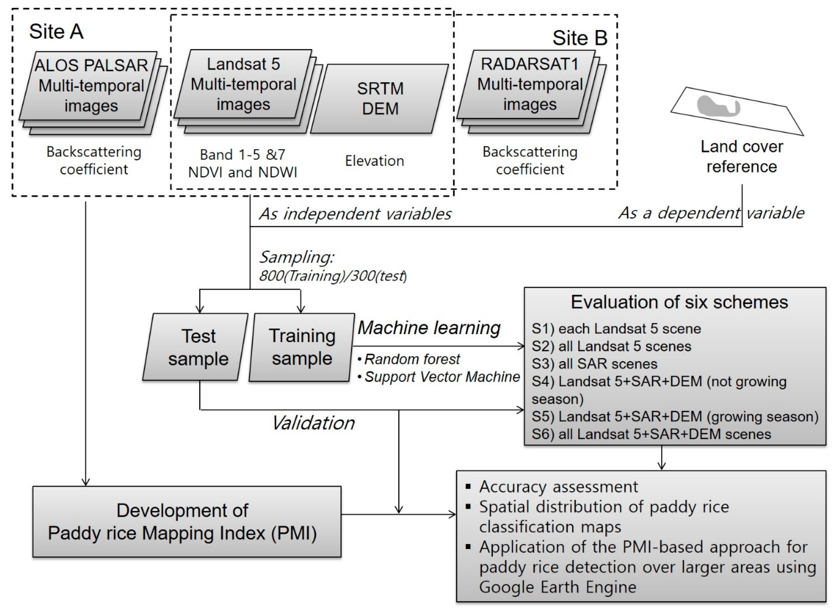
A total of 10 input variables—Landsat bands 1–5 and 7, NDVI, NDWI, SAR backscattering coefficients, and DEM—were used for paddy rice classification. Figure 3 shows a flowchart of this study. Classification models were constructed using training data through two machine learning approaches, RF and SVM.

RF is based on classification and regression trees (CART), which is a non-parametric model and constructs rule sets from data [42,43]. RF has two randomization processes, randomly selecting a subset of training samples (e.g., ~70%) for each tree and selecting a subset of variables at each node of a tree (e.g., squared root of the number of total variables). RF consists of many decision trees (the number of trees is 1000 in this study), and each tree has a decision. Finally, the class of an unknown pixel is determined through the majority voting of the results of trees. RF has been successfully conducted for various classification tasks in the literature [38,44,45,46,47,48,49,50,51]. RF also provides information about relative variable importance. Relative variable importance is based on an increased mean squared error (MSE) using out-of-bag data (i.e., unused training samples for each tree), which is calculated when randomly permuting an independent variable [52,53]. In this study, RF was implemented by R software (https://www.r-project.org/) through Random forest package with default settings (i.e., the number of randomly sampled variables as candidates at each split is the square root of the number of input variables; the minimum size of the terminal node is 1), except for the number of trees.

SVM is a supervised non-parametric approach and has been used in many studies in the remote sensing field [54,55,56,57,58,59,60]. The use of SVM has significantly increased because it works well in cases of limited training data sets and produces higher accuracy than other traditional approaches, such as Maximum Likelihood (ML) [61,62]. SVM conducts classification by determining hyperplanes that optimally separates classes [63]. One hyperplane only separates two classes so multiple hyperplanes are used to classify multiple classes. Kernel functions are typically adopted to transform the data dimensionality to make it easy to identify optimum hyperplanes. There are various kernel functions including linear, polynomial, radial basis function (RBF), and sigmoid [64]. This study used RBF kernel, widely used in classification tasks, and a grid-search method was used to determine the optimum values of parameters (i.e., gamma in the kernel function and penalty parameter) [65,66].

In this study, six schemes were tested to identify the improvement of classification performance when fusing multi-sensor time series data. Accuracy assessment was conducted under each scenario using test data (300 samples). Overall accuracies of multi-class classification (six classes for site A and eight classes for site B) and binary classification (i.e., paddy rice vs. non-paddy rice) were calculated for six schemes. The six schemes were designed considering sensor types and collection dates.

• Scheme 1 (S1): only Landsat data on each date were used for classification.
• Scheme 2 (S2): only Landsat data on all dates were used for classification.
• Scheme 3 (S3): only SAR data on all dates were used for classification.
• Scheme 4 (S4): Landsat, SAR, and DEM data during no growing season (November to March) were used for classification.
• Scheme 5 (S5): Landsat, SAR, and DEM data during the growing season (April to October) were used for classification.
• Scheme 6 (S6): Landsat, SAR, and DEM data on all dates were used for classification.

In order to evaluate the significant difference between classifications, the McNemar test, a non-parametric test based on the proportion correct/incorrect was conducted. Large error matrices can be collapsed to a binary size (i.e., 2 × 2) as the binary distinction between correct and incorrect class allocations should be focused for comparison [67,68]. The standardized normal test statistics (z) from the McNemar test is calculated as:

$$z=\frac{{\mathrm{f}}_{\mathrm{AB}}-{\mathrm{f}}_{\mathrm{BA}}}{\sqrt{{\mathrm{f}}_{\mathrm{AB}}+{\mathrm{f}}_{\mathrm{BA}}}}$$

(4)

where f_AB indicates the samples correctly identified in classification A, but is incorrectly classified in classification B; and, f_BA means the samples correctly identified in classification B, but incorrectly classified in classification A. The 5% level of significance (α = 0.05) was used for the McNemar test.

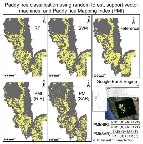
Important spectral and temporal characteristics for paddy rice classification were identified from the temporal pattern of each variable and variable importance, as provided by RF. In this study, Paddy rice Mapping Index (PMI) was proposed by considering the phenological characteristics of paddy rice in NIR and SAR backscattering coefficients. NIR reflectance and SAR backscattering coefficients are low during the planting/transplanting season (May) and increase during the growing season (Figure 4 and Figure 5). Paddy rice maps were produced from two classification models and PMI. The spatial distribution of the paddy rice maps was also compared with the reference paddy rice maps. PMI-based paddy rice mapping over a larger area (i.e., entire California State) was also conducted using Google Earth Engine.

4. Results

4.1. Evaluation of Paddy Rice Classification

Table 4. Summary of classification accuracies (%) at site A. The highest accuracy identified by model and classification type (i.e., multiclass vs. binary) is shown in bold.

	Multiclass Classification				Binary Classification
	RF		SVM		RF		SVM
	OA (%)	Kappa Coefficient	OA (%)	Kappa Coefficient	OA (%)	Kappa Coefficient	OA (%)	Kappa Coefficient
Scheme 1
15 January	75.00	0.64	76.00	0.65	85.00	0.68	86.00	0.70
31 January	76.33	0.65	80.67	0.72	85.33	0.69	89.33	0.77
20 March	84.33	0.77	85.67	0.79	94.67	0.89	96.67	0.93
2 April	66.00	0.51	72.00	0.59	78.67	0.56	81.33	0.61
5 April	83.33	0.76	87.67	0.82	95.00	0.89	95.67	0.91
21 April	84.67	0.78	86.00	0.80	95.67	0.91	96.33	0.92
7 May	85.33	0.79	88.00	0.83	97.00	0.94	98.33	0.96
23 May	85.00	0.78	87.00	0.81	99.67	0.99	99.67	0.99
8 June	86.33	0.80	90.33	0.86	98.33	0.96	99.00	0.98
24 June	85.00	0.78	87.67	0.82	98.33	0.96	97.67	0.95
10 July	86.33	0.80	88.67	0.84	98.33	0.96	99.00	0.98
26 July	86.33	0.80	91.33	0.87	98.67	0.97	100.00	1.00
27 August	86.67	0.81	88.67	0.84	96.67	0.93	97.67	0.95
7 September	73.67	0.62	75.67	0.65	88.67	0.76	89.67	0.77
30 October	82.33	0.74	82.67	0.75	90.33	0.80	89.67	0.78
15 November	84.33	0.77	85.33	0.79	93.67	0.87	94.67	0.89
Scheme 2	92.33	0.89	94.33	0.92	100.00	1.00	99.33	0.99
Scheme 3	80.00	0.71	78.33	0.69	90.67	0.80	91.33	0.81
Scheme 4	93.33	0.90	93.00	0.90	99.33	0.99	98.33	0.96
Scheme 5	90.00	0.85	92.33	0.89	99.67	0.99	99.33	0.99
Scheme 6	94.33	0.92	95.00	0.93	100.00	1.00	100.00	1.00

and

Table 5. Summary of classification accuracies (%) at site B. The highest accuracy identified by model and classification type (i.e., multiclass vs. binary) is shown in bold.

	Multiclass Classification				Binary Classification
	RF		SVM		RF		SVM
	OA (%)	Kappa Coefficient	OA (%)	Kappa Coefficient	OA (%)	Kappa Coefficient	OA (%)	Kappa Coefficient
Scheme 1
12 February	73.00	0.65	74.67	0.68	87.33	0.72	87.00	0.71
13 March	77.33	0.71	77.00	0.71	91.33	0.81	90.67	0.79
18 March	79.33	0.74	80.00	0.74	91.33	0.81	91.33	0.81
29 March	77.33	0.71	77.00	0.70	88.00	0.73	85.67	0.69
31 March	81.67	0.77	81.67	0.77	91.33	0.81	92.00	0.82
30 April	81.67	0.77	82.33	0.78	95.67	0.90	95.00	0.89
1 June	82.67	0.78	83.67	0.79	96.67	0.92	97.33	0.94
3 June	84.33	0.80	84.00	0.80	98.67	0.97	98.00	0.95
21 September	81.67	0.77	81.33	0.76	95.00	0.88	95.67	0.90
9 October	80.33	0.75	81.33	0.76	92.67	0.83	95.00	0.88
12 December	76.33	0.70	76.67	0.70	90.00	0.78	90.00	0.78
Scheme 2	86.33	0.83	88.67	0.86	98.00	0.95	99.33	0.98
Scheme 3	71.67	0.64	72.67	0.65	89.33	0.76	90.67	0.78
Scheme 4	84.67	0.80	85.67	0.82	94.00	0.86	94.67	0.88
Scheme 5	88.00	0.85	87.00	0.84	97.67	0.95	97.67	0.95
Scheme 6	88.00	0.85	87.67	0.84	98.00	0.95	98.67	0.97

show the accuracy assessment results of each approach for both multi-class and binary classifications. This experiment is repeated for 10 times, and the highest overall accuracy and kappa coefficient are shown in Table 4 and Table 5. In scheme 1, summer season data showed high accuracy in both sites because of the greenness of the paddy rice. While schemes 2 and 6 showed the highest accuracy in site A (100% and 1.00) and site B (99.33% and 0.99). It is not surprising that the accuracy is high when using time series data since they provide the phenology information of paddy rice. The use of SAR data only (i.e., scheme 3) did not work well for paddy rice classification, resulting in relatively low accuracy (~91%). The McNemar test results showed that there was a significant difference between scheme 3 and the other schemes for both sites (

Table 6. Summary of McNemar test results (|z|-values) of binary classifications for site A. The best classification for scheme 1 was used. |Z|-values are in bold if significantly different using α = 0.05.

	S1RF	S1SVM	S2RF	S2SVM	S3RF	S3SVM	S4RF	S4SVM	S5RF	S5SVM	S6RF	S6SVM
S1RF	-	-	-	-	-	-	-	-	-	-	-	-
S1SVM	2.00	-	-	-	-	-	-	-	-	-	-	-
S2RF	2.00	0.00	-	-	-	-	-	-	-	-	-	-
S2SVM	0.81	1.41	1.41	-	-	-	-	-	-	-	-	-
S3RF	4.54	5.29	5.29	4.75	-	-	-	-	-	-	-	-
S3SVM	4.02	5.10	5.10	4.54	0.45	-	-	-	-	-	-	-
S4RF	0.81	1.41	1.41	0.00	4.91	4.71	-	-	-	-	-	-
S4SVM	0.38	2.24	2.24	1.73	4.42	4.04	1.73	-	-	-	-	-
S5RF	1.34	1.00	1.00	0.58	5.01	4.81	0.58	1.63	-	-	-	-
S5SVM	0.82	1.41	1.41	0.00	4.91	4.71	0.00	1.34	1.00	-	-	-
S6RF	2.00	0.00	0.00	1.41	5.29	5.10	1.41	2.24	1.00	1.41	-	-
S6SVM	2.00	0.00	0.00	1.41	5.29	5.10	1.41	2.24	1.00	1.41	0.00	-

and

Table 7. Summary of McNemar test results (|z|-values) of binary classifications for site B. The best classification for scheme 1 was used. |Z|-values are in bold if significantly different using α = 0.05.

	S1RF	S1SVM	S2RF	S2SVM	S3RF	S3SVM	S4RF	S4SVM	S5RF	S5SVM	S6RF	S6SVM
S1RF	-	-	-	-	-	-	-	-	-	-	-	-
S1SVM	1.00	-	-	-	-	-	-	-	-	-	-	-
S2RF	0.82	0.00	-	-	-	-	-	-	-	-	-	-
S2SVM	1.41	2.00	2.00	-	-	-	-	-	-	-	-	-
S3RF	5.52	5.06	5.49	5.84	-	-	-	-	-	-	-	-
S3SVM	5.60	5.15	5.43	5.78	1.51	-	-	-	-	-	-	-
S4RF	3.13	2.56	2.83	3.58	3.33	3.28	-	-	-	-	-	-
S4SVM	2.83	2.24	2.36	3.30	3.48	3.78	0.63	-	-	-	-	-
S5RF	1.34	2.00	0.58	2.24	5.10	5.19	2.40	2.06	-	-	-	-
S5SVM	1.13	1.41	0.45	2.24	5.10	5.06	2.30	1.96	0.00	-	-	-
S6RF	0.82	0.00	0.00	2.00	5.49	5.43	2.83	2.36	0.58	0.44	-	-
S6SVM	0.00	0.82	1.41	1.41	5.67	5.60	3.13	2.83	1.73	1.73	1.41	-

). It is because scheme 3 uses SAR data of all dates only for classification and showed worse accuracy than the other schemes, which indicates that optical sensor data are crucial for paddy rice classification. In site B, scheme 5 showed a significantly higher accuracy than scheme 4, which implies that data from the growing season would be more contributing than data from the no growing season (from November to March) for paddy rice classification.

There is no big difference in classification accuracy by classification model. The McNemar test also showed that there was no significant difference between RF and SVM classifications (Table 6 and Table 7). However, the accuracy of SVM was slightly higher (~1–3%) than that of RF at both of the sites. The producer’s accuracy (PA) and user’s accuracy (UA) of SVM were also higher than RF (Supplementary Tables S1 and S2). The classification accuracies for site A (95% (0.93) in multiclass classification, 100% (1.00) in binary classification) were higher than those for site B (88.67% (0.86) in multiclass classification, 99.33% (0.98) in binary classification). The PA and UA in site A were also higher than those in site B (Supplementary Tables S1 and S2). In comparison with site A, site B is very cloudy during summer due to the Asian Monsoon, so there were not enough Landsat data for site B during summer which is important to classify land cover and paddy rice.

4.2. Analysis of Temporal and Spectral Characteristics of Paddy Rice

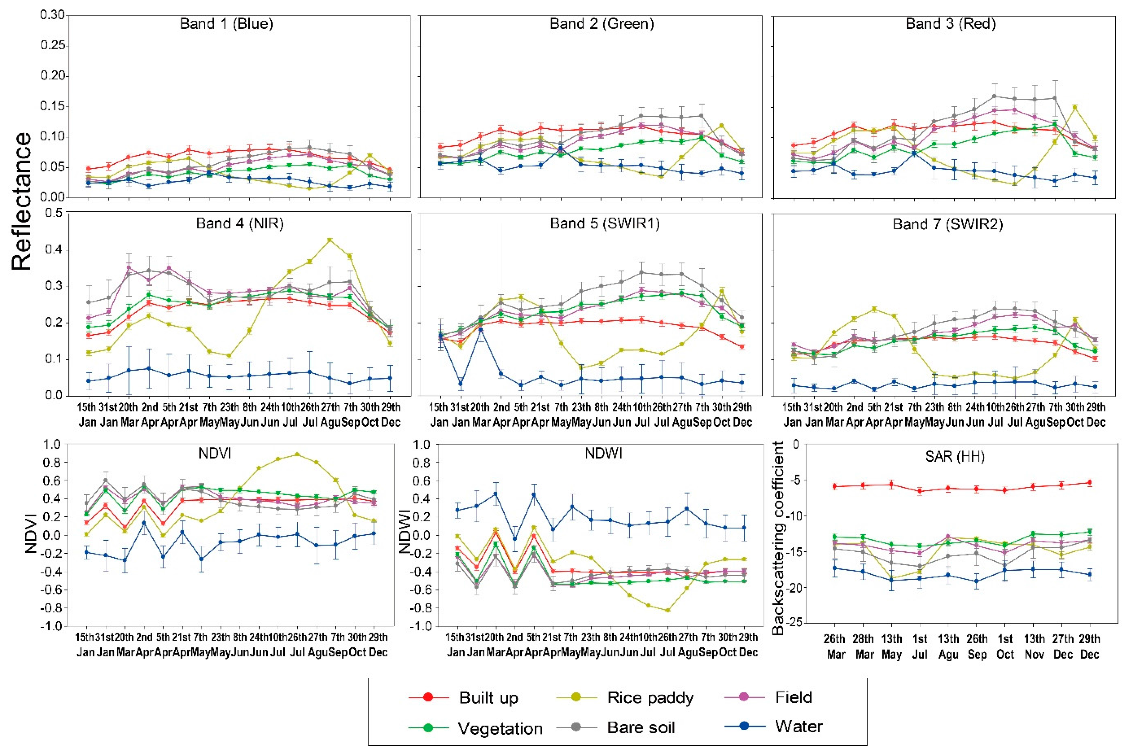
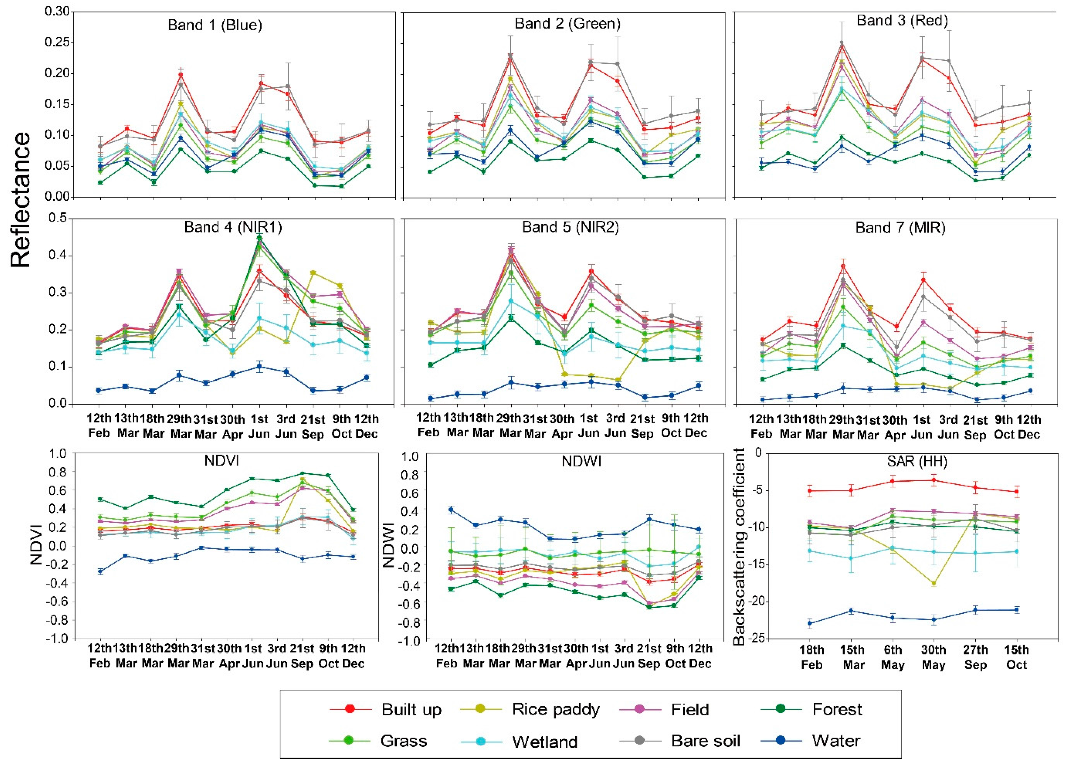
Figure 4 and Figure 5 shows the temporal patterns of nine variables (visible, NIR and SWIR bands, and SAR backscattering) for each land cover class at sites A and B, respectively. Although atmospheric correction was conducted through ENVI FLAASH, there are some fluctuations (Figure 5). This is because the graphs are not in order of years, but in order of months to better show both the phenological and spectral patterns of the paddy rice (refer to Table 1 and Table 2). Fluctuant patterns are more visible at site B, as it suffers from more severe atmospheric affects (e.g., clouds, fogs) than site A. Built-up class (refer to Table 3) generally results in a flat temporal pattern (Figure 4), but there are outliers in the built up class on 29 March, 1 June, and 3 June due to the atmospheric effect (Figure 5). SAR backscattering coefficients were not relatively affected by atmospheric conditions and the order of years with the flat temporal pattern in built-up class (Figure 4 and Figure 5).

There are no noticeable temporal characteristics in the visible bands (bands 1–3). The reflectance is low and shows typical characteristics, including the highest reflectance in built up areas, and the lowest reflectance in water. The reflectance of paddy rice and vegetation (e.g., field, forest, grass) increase in the NIR band during their growing season. In paddy rice, the reflectance of the NIR band shows a peak in August when photosynthesis is most active, and decreases in September to October when the color of paddy rice turns yellow (Figure 4 and Figure 5). SWIR2 is sensitive to leaf water content, and the more leaf water content there is, the lower the reflectance of SWIR2 is. Paddy rice shows the lowest reflectance of SWIR2 during the growing season, including the transplanting season (May) when the paddy is flooded (Figure 4 and Figure 5).

NDVI increases during the growing season in vegetation (paddy rice, grass, field, and forest), and paddy rice especially grows after transplanting (May). Contrary to NDVI, NDWI sensitive to water deficit during the growing season in vegetation. SAR backscattering shows the lowest roughness in water and the highest (brightest) in built up. Paddy rice shows a distinct phenological pattern in comparison with other land cover classes because paddy rice is flooded during the planting (transplanting) season, unlike other vegetation classes that have a continuously increased/decreased pattern (Figure 4 and Figure 5).

While paddy rice is distinguishable between July and September at site A, vegetation related classes (paddy rice, field, forest, and grass) show a similar pattern in NIR, MIR2, NDVI, and NDWI at site B. This is because sites A and B have different climatic and environmental characteristics: data availability due to clouds (site B has a high cloud cover rate) and the composition of land cover, especially in vegetation types (site B has more forests and denser vegetation areas than site A). However, the difference between planting and harvest seasons of paddy rice is distinct in both sites, and the characteristics of paddy rice are well depicted, especially in NIR spectral bands and SAR backscattering coefficients.

4.3. Paddy Rice Mapping Index (PMI)

PMI was developed when considering the phenological characteristics of paddy rice in terms of NIR and SAR backscattering coefficients (Equations (5) and (6)). PMI means the slope of NIR or SAR backscattering coefficients between the transplanting and harvest seasons because the difference of NIR and SAR backscattering coefficients between the two seasons in paddy rice is much higher than other classes. Since optical sensor data has higher data availability at a lower cost than SAR data, NIR based PMI might have a higher practicality than SAR based PMI.

$$\mathrm{PMI}(\mathrm{NIR})=\frac{\mathrm{NIR}1\left(\mathrm{Harvest}\right)-\mathrm{NIR}1\left(\mathrm{transplanting}\right)}{\mathrm{NIR}1\left(\mathrm{Harvest}\right)+\mathrm{NIR}1\left(\mathrm{transplanting}\right)}$$

(5)

$$\mathrm{PMI}(\mathrm{SAR})=\frac{\mathrm{SAR}\left(\mathrm{Harvest}\right)-\mathrm{SAR}\left(\mathrm{transplanting}\right)}{\mathrm{SAR}\left(\mathrm{Harvest}\right)+\mathrm{SAR}\left(\mathrm{transplanting}\right)}$$

(6)

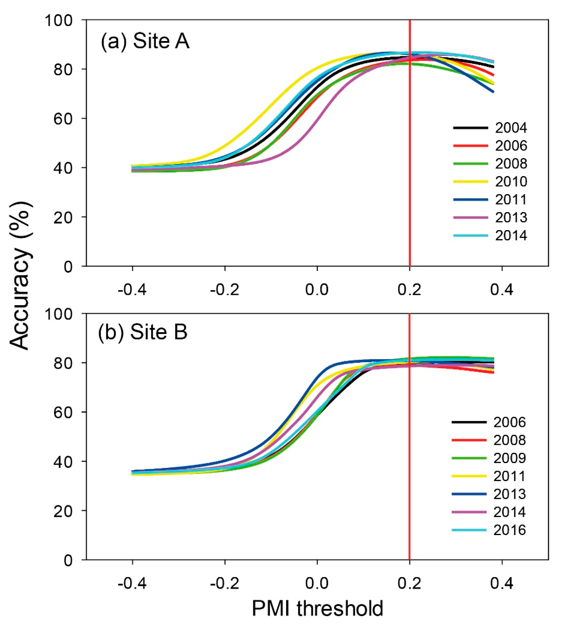
Since PMI is related to the probability of a pixel being paddy rice, it is necessary to determine an optimum threshold to identify paddy rice areas. The optimization of the threshold of NIR based PMI was conducted using reference data for the entire study areas (3,354,085 pixels at site A and 2,694,510 pixels at site B) based on the overall accuracy of binary classification (paddy rice or non-paddy rice). The optimization of SAR based PMI was not conducted due to the limited number of time series data. Figure 6 shows the change of accuracy with increasing thresholds of NIR-based PMI from −0.4 to 0.4 at interval of 0.02 for 13 years for both sites A and B (from 2004 to 2016). There are missing years due to clouds. PMI was calculated using NIR images from Landsat 5, 7, and 8. The highest accuracies were achieved when the threshold was near 0.2 for 10 years at both sites. Site A (~85%) shows higher accuracy than site B (~80%) because site A consisted of relatively homogeneous land cover, as discussed above. Figure 6c shows the box plot of optimal thresholds for 13 years at both of the sites. We determined 0.2 to be the optimal threshold of PMI, and a pixel is determined to be paddy rice when the PMI value of the pixel is greater than 0.2. In addition, it should be noted that the accuracy did not change much with the thresholds between 0.18–0.22 for both sites.

4.4. Spatial Distributions of Paddy Rice Maps

4.4.1. Comparisons of Spatial Distributions of Paddy Rice Maps

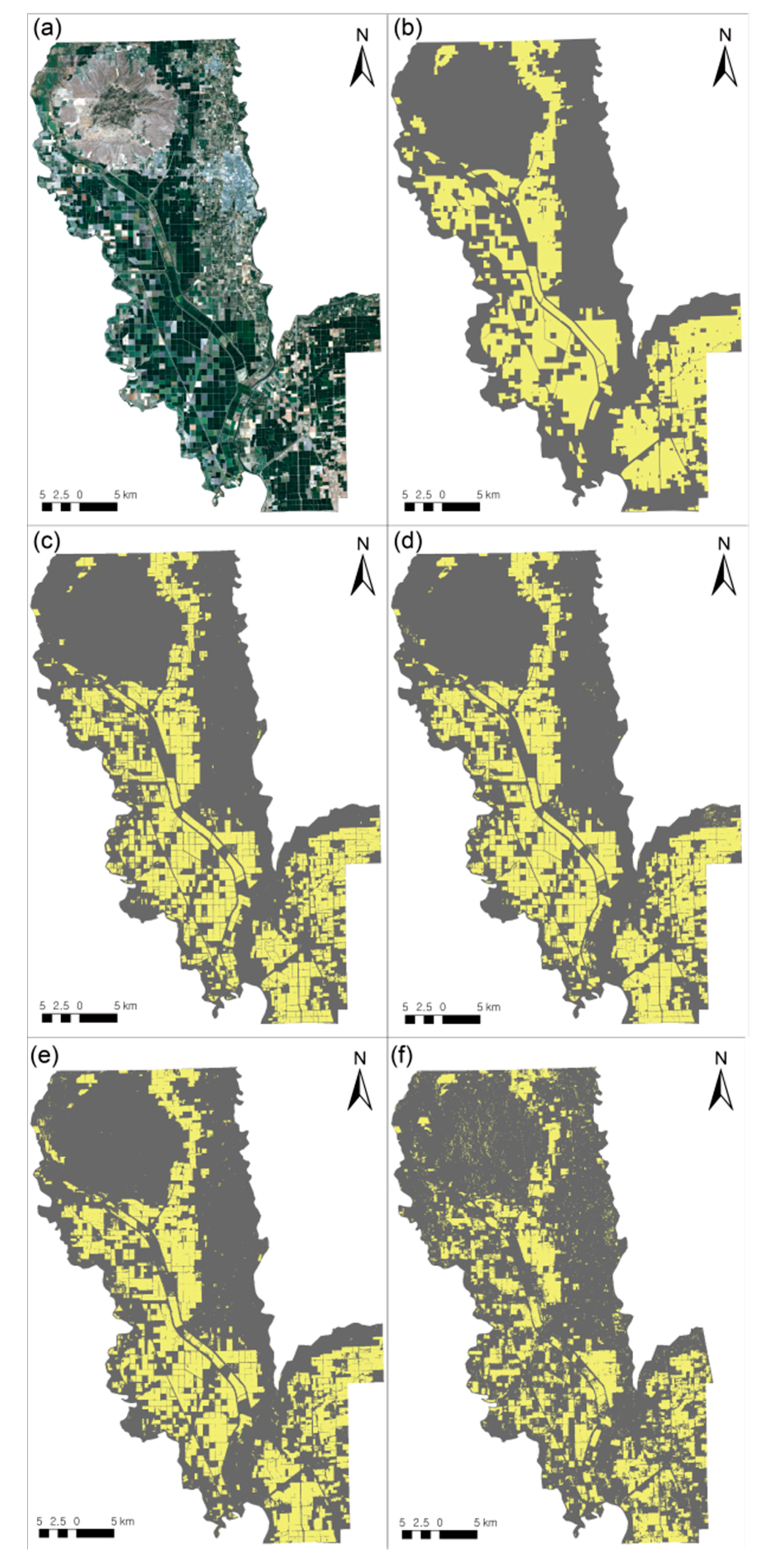
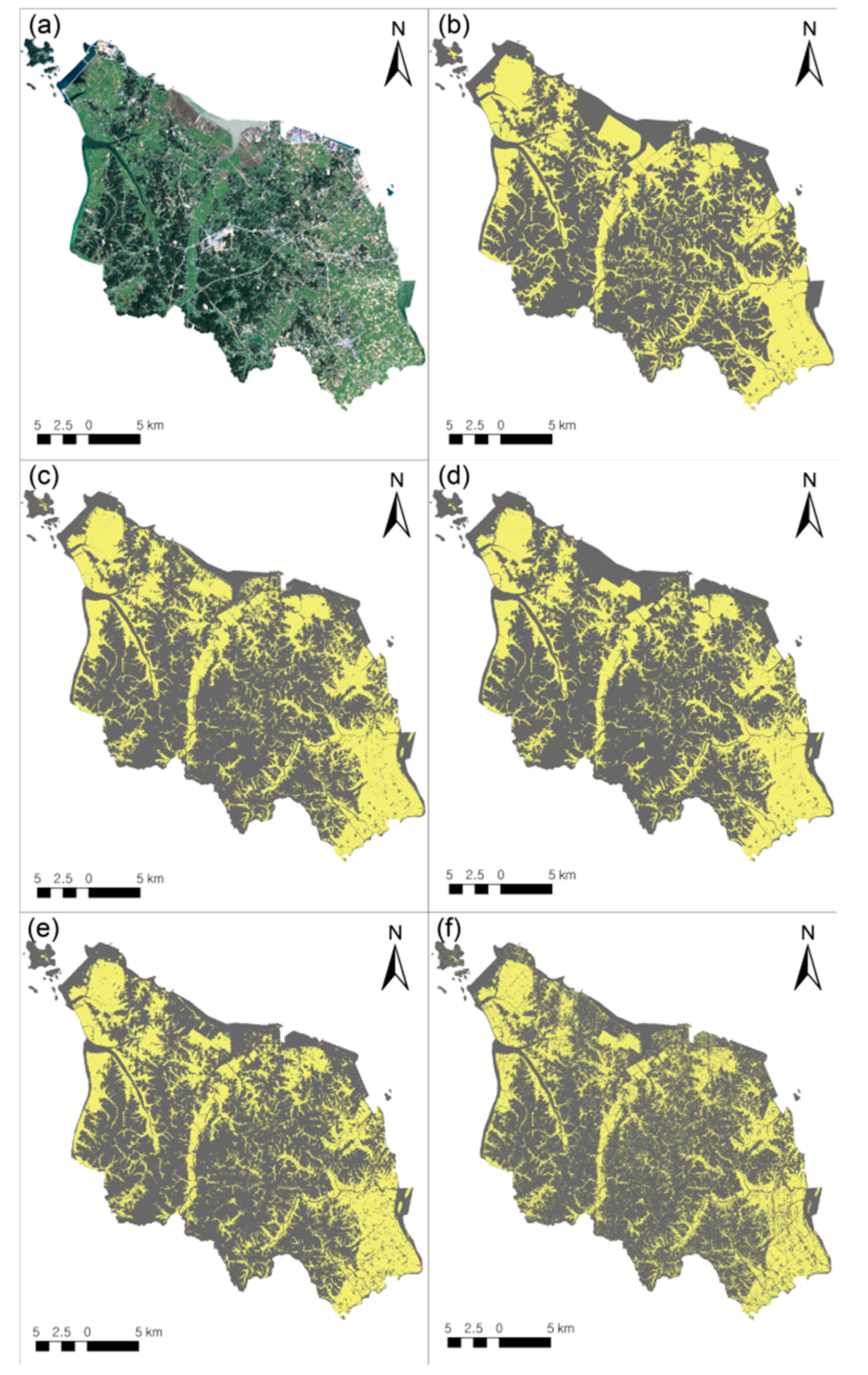
The visual comparison of paddy rice maps from RF-, SVM-, PMI (NIR)-, and PMI (SAR)-derived classification at both sites appears in Figure 7 and Figure 8. Machine learning-based paddy rice maps (Figure 7c,d and Figure 8c,d) were produced through scheme 6, which resulted in the best performance among the six schemes (Table 4 and Table 5) using RF and SVM classifiers. There is not much difference between two classifiers at site A, while the SVM result shows clearer paddy rice parcels than RF at site B. Paddy rice was not well detected and underestimated at site B because paddy rice and field are mixed within a pixel, especially at site B (Figure 8c–f).

PMI based paddy rice maps were calculated using NIR and SAR backscattering coefficients (Equations (5) and (6)) and, the thresholds applied were 0.2 (NIR) and −0.15 (SAR). The threshold of SAR based PMI was not fully optimized because the availability of time series of SAR data was very limited, so the threshold, (−0.15), was derived by averaging one year PMI optimized thresholds from two sites. SAR based PMI produced more noisy paddy rice maps than NIR based PMI due to speckle, which is one of the limitations of SAR images [69]. The overall accuracy of binary classification (paddy rice or non-paddy rice) for the entire study areas (3,354,085 pixels at site A and 2,694,510 pixels at site B) was calculated. That classification results with two machine learning classifiers (~95% at site A and ~90% at site B) were more accurate than PMI (NIR) based results (~87% at site A and ~83% at site B).

4.4.2. PMI-Based Paddy Rice Mapping Using Google Earth Engine

PMI was applied to a larger area (paddy rice cultivated area in California State; Figure 9) using the threshold of 0.2. Figure 9 shows PMI based paddy rice maps on the Google Earth Engine platform. The reference paddy rice map was obtained from USDM CDL 2016. Paddy rice was well detected through PMI, although there were some false alarms that were caused by clouds. These results indicate that PMI can effectively map and monitor yearly paddy rice areas at a national or larger scale through Google Earth Engine through the improvement of computing capacity. We also tested the PMI-based paddy rice mapping for other regions where rice is cultivated (Pohang in South Korea, Acadia county in Louisiana State, and Arkansas county in Arkansas state, United State; Supplementary Figure S1). Paddy rice was well detected through PMI where the fields are flooded during the transplanting season (Pohang and Acadia County).

5. Discussion

Paddy rice classification was conducted by expanding the dimensionality of data on both spectral and temporal domains using two machine learning approaches, RF and SVM. The six schemes that were composed of various combinations of input data by sensor and collection date were carried out, and the effect of data dimensionality was analyzed over two different regions. The spectral and temporal characteristics of paddy rice were identified, and Paddy rice Mapping Index (PMI) was proposed based on the phenological characteristics of paddy rice.

SAR data contributed to paddy rice classification more for site A than site B, which implies that it might not be ideal to use SAR data only for paddy rice classification in areas with rugged terrains and heterogeneous land cover. Nonetheless, SAR data were able to improve classification accuracy when using with Landsat data. Although it is considered that the fusion of Landsat and SAR might not be necessary for areas with low cloud cover, such a fusion can be effective to paddy rice classification for Asia because most regions in Asia are very cloudy, especially for the growing season, which limits the availability of optical time series data.

The performance of SVM was better than that of RF at both sites, which is consistent with Pouteau et al. [70] and Raczko & Zagajewski [71]. In this study, classifications were conducted in a 10-dimensional feature space for scheme 1, and more than 60-dimensional feature space for the other schemes. As SVM is known to work well in a large dimensional feature space, it could be better for SVM to classify paddy rice than RF [70]. Raczko and Zagajewski [71] stated that the number of training samples has an impact on the performance of a classifier, and Kavzoglu & Mather [72] stated that more than 400 pixels per class are needed for robust classification. In this study, a relatively small number of training samples (less than 200 pixels per class) were used, which might explain the better performance of SVM than RF because SVM works well with a small sample size as well as mixed pixels [56,73].

Land cover was more heterogeneous in site B than site A with a higher number of classes (six classes in site A and eight classes in site B). The population density of site B (249 people/km²) was about four times more than that of site A (61 people/km²), and classes were more patched and thus more mixed within a pixel in site B than site A. Those factors influenced the classification accuracy at site B. The size of paddy rice fields needs to be considered in the future research as discussed in Dong et al. [17]. Higher resolution data, such as RapidEye, are needed to classify paddy rice where the size of paddy rice field is small, such as in site B.

The approach proposed in this study have benefited from the use of phenological characteristics of paddy rice (i.e., time series data). The phenology of paddy rice in terms of various spectral bands and vegetation indices can be used for numerous applications because such phenology is a relative characteristic that varies by region. There are many fields that use the phenological characteristics of crops (e.g., paddy rice), such as classifying different vegetation (crop) types [74,75], crop yield estimation [76,77], gross and net primary production (GPP/NPP) estimation [78], and quantifying crop water requirements [79]. In addition, the approach that was developed in this study can be applied to any inaccessible regions where in situ data are not available, such as North Korea. For example, previous studies conducted classification over inaccessible regions applying training samples from different areas that have similar climate and environmental characteristics [80] or unsupervised classification [81].

While machine learning-based classification requires training data, which is often challenging for certain areas, PMI-based paddy rice mapping does not require any in situ data for training. Although the validation accuracy of PMI based results was relatively lower than those of the machine learning approaches, the spatial distribution of paddy rice well matched that of the reference paddy rice data. PMI can be applied to different regions with the same threshold (greater than 0.2) or an adjusted threshold considering the dates of data acquisition. Consequently, PMI is considered to be useful to map paddy rice because PMI is calculated using a very simple equation and needs only two Landsat images or similar satellite data with NIR bands during the planting and harvest seasons. An annual update of paddy rice maps is possible using PMI. However, the availability of optical sensor data due to cloud contamination could be a limiting factor, especially for East Asia. This limitation can be overcome using geostationary satellite data, such as planned Geostationary Ocean Color Imager (GOCI)-2, which have high temporal resolution (~hourly) with 250 m spatial resolution. It is expected that fully clear images during two seasons can be successfully obtained every year using geostationary satellite data.

Paddy rice mapping at a regional or continental scale can be conducted using PMI through Google Earth Engine with an aid of the continued improvement of computing capacity. However, in this study, paddy rice detected using PMI was somewhat confused with other crops where paddy rice is planted in dry fields. It is one of the limitations of using PMI, in that PMI can be successfully applied only where paddy rice is planted in flooded fields.

6. Conclusions

As the population in the world increases, the demand of rice also increases. Thus, providing accurate and up-to-date paddy rice maps is very important. A satellite-based approach produces paddy rice maps with a fast update cycle in comparison with the traditional survey approach. In this study, Landsat, SAR, and SRTM data were used to classify paddy rice at two sites that have different climatic and environmental characteristics. This study evaluated six schemes to identify the improvement of classification performance through the investigation of the characteristics of study areas, classifiers, and fusion of multi-sensor time series data. As expected, the classification accuracy was the highest when using multi-sensor time series data (scheme 6). Site A showed better performance than site B because Site A consisted of more homogeneous land cover and had higher data availability during the growing season than site B. The performance of SVM classifier was slightly better (accuracy of 1–3%) than RF, especially at site B because SVM works well in a small sample size and at a mixed pixel. Paddy Rice Mapping Index (PMI) considering spectral and phenological characteristics of paddy rice was proposed in this study. NIR and SAR backscattering coefficients detected the phenological characteristic of paddy rice well. Although the performance of PMI is slightly worse than the RF or SVM classifications based on multi-sensor time series data, PMI is useful to operationally map paddy rice, because PMI is simply calculated only using two scenes and does not require training data, which implies that the PMI-based approach can be applied to different regions. In addition, paddy rice can be easily mapped using the Google Earth Engine platform.

There are some limitations in the use of PMI. PMI can be applied only where paddy rice areas are flooded during the transplanting season. As the current threshold, greater than 0.21, based on the results for 13 years is a little arbitrary, more robust and adaptive thresholding approaches should be considered. There are some misclassified pixels due to the heterogeneous composition of the land cover within a pixel at site B. In further studies, the size of paddy rice fields need to be considered when selecting satellite images, and higher resolution data, such as RapidEye or Worldview series, need to be evaluated to detect small size paddy rice patches.

References

- Karila, K.; Nevalainen, O.; Krooks, A.; Karjalainen, M.; Kaasalainen, S. Monitoring changes in rice cultivated area from SAR and optical satellite images in Ben Tre and Tra Vinh Provinces in Mekong Delta, Vietnam. Remote Sens. 2014, 6, 4090–4108. [Google Scholar] [CrossRef]
- Mohanty, S.; Wassmann, R.; Nelson, A.; Moya, P.; Jagadish, S. Rice and climate change: Significance for food security and vulnerability. Int. Rice Res. Inst. 2013, 14, 1–12. [Google Scholar]
- Purevdorj, M.; Kubo, M. The future of rice production, consumption and seaborne trade: Synthetic prediction method. J. Food Distrib. Res. 2005, 36, 250–259. [Google Scholar]
- Muthayya, S.; Sugimoto, J.D.; Montgomery, S.; Maberly, G.F. An overview of global rice production, supply, trade, and consumption. Ann. N. Y. Acad. Sci. 2014, 1324, 7–14. [Google Scholar] [CrossRef] [PubMed]
- Mosleh, M.K.; Hassan, Q.K.; Chowdhury, E.H. Application of remote sensors in mapping rice area and forecasting its production: A review. Sensors 2015, 15, 769–791. [Google Scholar] [CrossRef] [PubMed]
- Yuanshu, J.; Gen, L.; Jianjun, C.; Yiwen, S. Determination of paddy rice growth indicators with MODIS data and ground-based measurements of LAI. In Proceedings of the 2013 the International Conference on Remote Sensing, Environment and Transportation Engineering (RSETE 2013), Nanjing, China, 26–28 July 2013. [Google Scholar]
- Fang, H.; Wu, B.; Liu, H.; Huang, X. Using NOAA AVHRR and Landsat TM to estimate rice area year-by-year. Int. J. Remote Sens. 1998, 19, 521–525. [Google Scholar] [CrossRef]
- Thenkabail, P.S.; Schull, M.; Turral, H. Ganges and Indus river basin land use/land cover (LULC) and irrigated area mapping using continuous streams of MODIS data. Remote Sens. Environ. 2005, 95, 317–341. [Google Scholar] [CrossRef]
- Jin, C.; Xiao, X.; Dong, J.; Qin, Y.; Wang, Z. Mapping paddy rice distribution using multi-temporal Landsat imagery in the Sanjiang Plain, northeast China. Front. Earth Sci. 2016, 10, 49–62. [Google Scholar] [CrossRef] [PubMed]
- Long, J.A.; Lawrence, R.L.; Greenwood, M.C.; Marshall, L.; Miller, P.R. Object-oriented crop classification using multitemporal ETM+ SLC-off imagery and random forest. GISci. Remote Sens. 2013, 50, 418–436. [Google Scholar]
- Xiao, X.; Boles, S.; Frolking, S.; Li, C.; Babu, J.Y.; Salas, W.; Moore, B. Mapping paddy rice agriculture in South and Southeast Asia using multi-temporal MODIS images. Remote Sens. Environ. 2006, 100, 95–113. [Google Scholar] [CrossRef]
- Gumma, M.K.; Nelson, A.; Thenkabail, P.S.; Singh, A.N. Mapping rice areas of South Asia using MODIS multitemporal data. J. Appl. Remote Sens. 2011, 5, 053547. [Google Scholar] [CrossRef]
- Nuarsa, I.W.; Nishio, F.; Hongo, C.; Mahardika, I.G. Using variance analysis of multitemporal MODIS images for rice field mapping in Bali Province, Indonesia. Int. J. Remote Sens. 2012, 33, 5402–5417. [Google Scholar] [CrossRef]
- Son, N.-T.; Chen, C.-F.; Chen, C.-R.; Duc, H.-N.; Chang, L.-Y. A phenology-based classification of time-series MODIS data for rice crop monitoring in Mekong Delta, Vietnam. Remote Sens. 2013, 6, 135–156. [Google Scholar] [CrossRef]
- Qin, Y.; Xiao, X.; Dong, J.; Zhou, Y.; Zhu, Z.; Zhang, G.; Du, G.; Jin, C.; Kou, W.; Wang, J. Mapping paddy rice planting area in cold temperate climate region through analysis of time series Landsat 8 (OLI), Landsat 7 (ETM+) and MODIS imagery. ISPRS J. Photogramm. Remote Sens. 2015, 105, 220–233. [Google Scholar] [CrossRef] [PubMed]
- Zhang, G.; Xiao, X.; Dong, J.; Kou, W.; Jin, C.; Qin, Y.; Zhou, Y.; Wang, J.; Menarguez, M.A.; Biradar, C. Mapping paddy rice planting areas through time series analysis of MODIS land surface temperature and vegetation index data. ISPRS J. Photogramm. Remote Sens. 2015, 106, 157–171. [Google Scholar] [CrossRef] [PubMed]
- Dong, J.; Xiao, X. Evolution of regional to global paddy rice mapping methods: A review. ISPRS J. Photogramm. Remote Sens. 2016, 119, 214–227. [Google Scholar] [CrossRef]
- Clauss, K.; Yan, H.; Kuenzer, C. Mapping Paddy Rice in China in 2002, 2005, 2010 and 2014 with MODIS Time Series. Remote Sens. 2016, 8, 434. [Google Scholar] [CrossRef]
- Dong, J.; Xiao, X.; Kou, W.; Qin, Y.; Zhang, G.; Li, L.; Jin, C.; Zhou, Y.; Wang, J.; Biradar, C. Tracking the dynamics of paddy rice planting area in 1986–2010 through time series Landsat images and phenology-based algorithms. Remote Sens. Environ. 2015, 160, 99–113. [Google Scholar] [CrossRef]
- Zhu, Z.; Woodcock, C.E.; Rogan, J.; Kellndorfer, J. Assessment of spectral, polarimetric, temporal, and spatial dimensions for urban and peri-urban land cover classification using Landsat and SAR data. Remote Sens. Environ. 2012, 117, 72–82. [Google Scholar] [CrossRef]
- Niu, X.; Ban, Y. Multi-temporal RADARSAT-2 polarimetric SAR data for urban land-cover classification using an object-based support vector machine and a rule-based approach. Int. J. Remote Sens. 2013, 34, 1–26. [Google Scholar] [CrossRef]
- Amarsaikhan, D.; Saandar, M.; Ganzorig, M.; Blotevogel, H.; Egshiglen, E.; Gantuyal, R.; Nergui, B.; Enkhjargal, D. Comparison of multisource image fusion methods and land cover classification. Int. J. Remote Sens. 2012, 33, 2532–2550. [Google Scholar] [CrossRef]
- Sheoran, A.; Haack, B. Classification of California agriculture using quad polarization radar data and Landsat Thematic Mapper data. GISci. Remote Sens. 2013, 50, 50–63. [Google Scholar]
- Xie, L.; Zhang, H.; Wu, F.; Wang, C.; Zhang, B. Capability of rice mapping using hybrid polarimetric SAR data. IEEE J. Sel. Top. Appl. Earth Obs. Remote Sens. 2015, 8, 3812–3822. [Google Scholar] [CrossRef]
- Stefanski, J.; Kuemmerle, T.; Chaskovskyy, O.; Griffiths, P.; Havryluk, V.; Knorn, J.; Korol, N.; Sieber, A.; Waske, B. Mapping land management regimes in western Ukraine using optical and SAR data. Remote Sens. 2014, 6, 5279–5305. [Google Scholar] [CrossRef]
- Torbick, N.; Chowdhury, D.; Salas, W.; Qi, J. Monitoring Rice Agriculture across Myanmar Using Time Series Sentinel-1 Assisted by Landsat-8 and PALSAR-2. Remote Sens. 2017, 9, 119. [Google Scholar] [CrossRef]
- Wang, J.; Xiao, X.; Qin, Y.; Dong, J.; Zhang, G.; Kou, W.; Jin, C.; Zhou, Y.; Zhang, Y. Mapping paddy rice planting area in wheat-rice double-cropped areas through integration of Landsat-8 OLI, MODIS, and PALSAR images. Sci. Rep. 2015, 5, 10088. [Google Scholar] [CrossRef] [PubMed]
- Kuenzer, C.; Knauer, K. Remote sensing of rice crop areas. Int. J. Remote Sens. 2013, 34, 2101–2139. [Google Scholar] [CrossRef]
- Dube, T.; Mutanga, O. Evaluating the utility of the medium-spatial resolution Landsat 8 multispectral sensor in quantifying aboveground biomass in uMgeni catchment, South Africa. ISPRS J. Photogramm. Remote Sens. 2015, 101, 36–46. [Google Scholar] [CrossRef]
- Matongera, T.N.; Mutanga, O.; Dube, T.; Lottering, R.T. Detection and mapping of bracken fern weeds using multispectral remotely sensed data: A review of progress and challenges. Geocarto Int. 2018, 33, 209–224. [Google Scholar] [CrossRef]
- Irons, J.R.; Dwyer, J.L.; Barsi, J.A. The next Landsat satellite: The Landsat data continuity mission. Remote Sens. Environ. 2012, 122, 11–21. [Google Scholar] [CrossRef]
- Zhang, Y.; Wang, C.; Wu, J.; Qi, J.; Salas, W.A. Mapping paddy rice with multitemporal ALOS/PALSAR imagery in southeast China. Int. J. Remote Sens. 2009, 30, 6301–6315. [Google Scholar] [CrossRef]
- Le Toan, T.; Ribbes, F.; Wang, L.-F.; Floury, N.; Ding, K.-H.; Kong, J.A.; Fujita, M.; Kurosu, T. Rice crop mapping and monitoring using ERS-1 data based on experiment and modeling results. IEEE Trans. Geosci. Remote Sens. 1997, 35, 41–56. [Google Scholar] [CrossRef]
- Shao, Y.; Fan, X.; Liu, H.; Xiao, J.; Ross, S.; Brisco, B.; Brown, R.; Staples, G. Rice monitoring and production estimation using multitemporal RADARSAT. Remote Sens. Environ. 2001, 76, 310–325. [Google Scholar] [CrossRef]
- Miyaoka, K.; Maki, M.; Susaki, J.; Homma, K.; Noda, K.; Oki, K. Rice-planted area mapping using small sets of multi-temporal SAR data. IEEE Geosci. Remote Sens. Lett. 2013, 10, 1507–1511. [Google Scholar] [CrossRef]
- Shimada, M.; Isoguchi, O.; Tadono, T.; Isono, K. PALSAR radiometric and geometric calibration. IEEE Trans. Geosci. Remote Sens. 2009, 47, 3915–3932. [Google Scholar] [CrossRef]
- Lee, J.-S. Digital image enhancement and noise filtering by use of local statistics. IEEE Trans. Pattern Anal. Mach. Intell. 1980, 2, 165–168. [Google Scholar] [CrossRef] [PubMed]
- Rodriguez-Galiano, V.F.; Ghimire, B.; Rogan, J.; Chica-Olmo, M.; Rigol-Sanchez, J.P. An assessment of the effectiveness of a random forest classifier for land-cover classification. ISPRS J. Photogramm. Remote Sens. 2012, 67, 93–104. [Google Scholar] [CrossRef]
- Zhou, W. An object-based approach for urban land cover classification: Integrating LiDAR height and intensity data. IEEE Geosci. Remote Sens. Lett. 2013, 10, 928–931. [Google Scholar] [CrossRef]
- Balzter, H.; Cole, B.; Thiel, C.; Schmullius, C. Mapping CORINE land cover from Sentinel-1A SAR and SRTM digital elevation model data using Random Forests. Remote Sens. 2015, 7, 14876–14898. [Google Scholar] [CrossRef]
- Johnson, D.M.; Mueller, R. The 2009 Cropland Data Layer. Photogramm. Eng. Remote Sens. 2010, 76, 1201–1205. [Google Scholar]
- Naidoo, L.; Cho, M.A.; Mathieu, R.; Asner, G. Classification of savanna tree species, in the Greater Kruger National Park region, by integrating hyperspectral and LiDAR data in a Random Forest data mining environment. ISPRS J. Photogramm. Remote Sens. 2012, 69, 167–179. [Google Scholar] [CrossRef]
- Prasad, A.M.; Iverson, L.R.; Liaw, A. Newer classification and regression tree techniques: Bagging and random forests for ecological prediction. Ecosystems 2006, 9, 181–199. [Google Scholar] [CrossRef]
- Pelletier, C.; Valero, S.; Inglada, J.; Champion, N.; Dedieu, G. Assessing the robustness of Random Forests to map land cover with high resolution satellite image time series over large areas. Remote Sens. Environ. 2016, 187, 156–168. [Google Scholar] [CrossRef]
- Griffiths, P.; van der Linden, S.; Kuemmerle, T.; Hostert, P. A pixel-based Landsat compositing algorithm for large area land cover mapping. IEEE J. Sel. Top. Appl. Earth Obs. Remote Sens. 2013, 6, 2088–2101. [Google Scholar] [CrossRef]
- Ghimire, B.; Rogan, J.; Galiano, V.R.; Panday, P.; Neeti, N. An evaluation of bagging, boosting, and random forests for land-cover classification in Cape Cod, Massachusetts, USA. GISci. Remote Sens. 2012, 49, 623–643. [Google Scholar] [CrossRef]
- Lawrence, R.L.; Wood, S.D.; Sheley, R.L. Mapping invasive plants using hyperspectral imagery and Breiman Cutler classifications (RandomForest). Remote Sens. Environ. 2006, 100, 356–362. [Google Scholar] [CrossRef]
- Waske, B.; Braun, M. Classifier ensembles for land cover mapping using multitemporal SAR imagery. ISPRS J. Photogramm. Remote Sens. 2009, 64, 450–457. [Google Scholar] [CrossRef]
- Richardson, H.J.; Hill, D.J.; Denesiuk, D.R.; Fraser, L.H. A comparison of geographic datasets and field measurements to model soil carbon using random forests and stepwise regressions (British Columbia, Canada). GISci. Remote Sens. 2017, 54, 573–591. [Google Scholar] [CrossRef]
- Amani, M.; Salehi, B.; Mahdavi, S.; Granger, J.; Brisco, B. Wetland classification in Newfoundland and Labrador using multi-source SAR and optical data integration. GISci. Remote Sens. 2017, 54, 779–796. [Google Scholar] [CrossRef]
- Guo, Z.; Du, S. Mining parameter information for building extraction and change detection with very high-resolution imagery and GIS data. GISci. Remote Sens. 2017, 54, 38–63. [Google Scholar] [CrossRef]
- Im, J.; Park, S.; Rhee, J.; Baik, J.; Choi, M. Downscaling of AMSR-E soil moisture with MODIS products using machine learning approaches. Environ. Earth Sci. 2016, 75, 1120. [Google Scholar] [CrossRef]
- Park, S.; Im, J.; Jang, E.; Rhee, J. Drought assessment and monitoring through blending of multi-sensor indices using machine learning approaches for different climate regions. Agric. For. Meteorol. 2016, 216, 157–169. [Google Scholar] [CrossRef]
- Foody, G.M.; Mathur, A. Toward intelligent training of supervised image classifications: Directing training data acquisition for SVM classification. Remote Sens. Environ. 2004, 93, 107–117. [Google Scholar] [CrossRef]
- Pal, M.; Mather, P. Support vector machines for classification in remote sensing. Int. J. Remote Sens. 2005, 26, 1007–1011. [Google Scholar] [CrossRef]
- Dalponte, M.; Ene, L.T.; Marconcini, M.; Gobakken, T.; Næsset, E. Semi-supervised SVM for individual tree crown species classification. ISPRS J. Photogramm. Remote Sens. 2015, 110, 77–87. [Google Scholar] [CrossRef]
- Yang, B.; Dong, Z.; Liu, Y.; Liang, F.; Wang, Y. Computing multiple aggregation levels and contextual features for road facilities recognition using mobile laser scanning data. ISPRS J. Photogramm. Remote Sens. 2017, 126, 180–194. [Google Scholar] [CrossRef]
- Li, X.; Zhang, C.; Li, W. Building block level urban land-use information retrieval based on Google Street View images. GISci. Remote Sens. 2017, 54, 819–835. [Google Scholar] [CrossRef]
- Wang, C.; Pavlowsky, R.T.; Huang, Q.; Chang, C. Channel bar feature extraction for a mining-contaminated river using high-spatial multispectral remote-sensing imagery. GISci. Remote Sens. 2016, 53, 283–302. [Google Scholar] [CrossRef]
- Chu, H.-J.; Wang, C.-K.; Kong, S.-J.; Chen, K.-C. Integration of full-waveform LiDAR and hyperspectral data to enhance tea and areca classification. GISci. Remote Sens. 2016, 53, 542–559. [Google Scholar] [CrossRef]
- Mantero, P.; Moser, G.; Serpico, S.B. Partially supervised classification of remote sensing images through SVM-based probability density estimation. IEEE Trans. Geosci. Remote Sens. 2005, 43, 559–570. [Google Scholar] [CrossRef]
- Mountrakis, G.; Im, J.; Ogole, C. Support vector machines in remote sensing: A review. ISPRS J. Photogramm. Remote Sens. 2011, 66, 247–259. [Google Scholar] [CrossRef]
- Huang, C.; Davis, L.; Townshend, J. An assessment of support vector machines for land cover classification. Int. J. Remote Sens. 2002, 23, 725–749. [Google Scholar] [CrossRef]
- Kavzoglu, T.; Colkesen, I. A kernel functions analysis for support vector machines for land cover classification. Int. J. Appl. Earth Obs. Geoinf. 2009, 11, 352–359. [Google Scholar] [CrossRef]
- Joachims, T. Learning to Classify Text Using Support Vector Machines: Methods, Theory and Algorithms; Kluwer Academic Publishers: Norwell, MA, USA, 2002. [Google Scholar]
- Shao, Y.; Lunetta, R.S. Comparison of support vector machine, neural network, and CART algorithms for the land-cover classification using limited training data points. ISPRS J. Photogramm. Remote Sens. 2012, 70, 78–87. [Google Scholar] [CrossRef]
- Foody, G.M. Thematic map comparison. Photogramm. Eng. Remote Sens. 2004, 70, 627–633. [Google Scholar] [CrossRef]
- Gong, B.; Im, J.; Mountrakis, G. An artificial immune network approach to multi-sensor land use/land cover classification. Remote Sens. Environ. 2011, 115, 600–614. [Google Scholar] [CrossRef]
- Joshi, N.; Baumann, M.; Ehammer, A.; Fensholt, R.; Grogan, K.; Hostert, P.; Jepsen, M.R.; Kuemmerle, T.; Meyfroidt, P.; Mitchard, E.T. A review of the application of optical and radar remote sensing data fusion to land use mapping and monitoring. Remote Sens. 2016, 8, 70. [Google Scholar] [CrossRef]
- Pouteau, R.; Meyer, J.-Y.; Taputuarai, R.; Stoll, B. Support vector machines to map rare and endangered native plants in Pacific islands forests. Ecol. Inf. 2012, 9, 37–46. [Google Scholar] [CrossRef]
- Raczko, E.; Zagajewski, B. Comparison of support vector machine, random forest and neural network classifiers for tree species classification on airborne hyperspectral APEX images. Eur. J. Remote Sens. 2017, 50, 144–154. [Google Scholar] [CrossRef]
- Kavzoglu, T.; Mather, P.M. The use of backpropagating artificial neural networks in land cover classification. Int. J. Remote Sens. 2003, 24, 4907–4938. [Google Scholar] [CrossRef]
- Foody, G.M.; Mathur, A. The use of small training sets containing mixed pixels for accurate hard image classification: Training on mixed spectral responses for classification by a SVM. Remote Sens. Environ. 2006, 103, 179–189. [Google Scholar] [CrossRef]
- Kim, H.-O.; Yeom, J.-M. Sensitivity of vegetation indices to spatial degradation of RapidEye imagery for paddy rice detection: A case study of South Korea. GISci. Remote Sens. 2015, 52, 1–17. [Google Scholar] [CrossRef]
- Ramoelo, A.; Skidmore, A.K.; Cho, M.A.; Schlerf, M.; Mathieu, R.; Heitkönig, I.M. Regional estimation of savanna grass nitrogen using the red-edge band of the spaceborne RapidEye sensor. Int. J. Appl. Earth Obs. Geoinf. 2012, 19, 151–162. [Google Scholar] [CrossRef]
- Kim, M.; Ko, J.; Jeong, S.; Yeom, J.-M.; Kim, H.-O. Monitoring canopy growth and grain yield of paddy rice in South Korea by using the GRAMI model and high spatial resolution imagery. GISci. Remote Sens. 2017, 54, 534–551. [Google Scholar] [CrossRef]
- Bouman, B. ORYZA2000: Modeling Lowland Rice; IRRI: Los Baños, Philippine, 2001; Volume 1. [Google Scholar]
- Ciais, P.; Reichstein, M.; Viovy, N.; Granier, A.; Ogée, J.; Allard, V.; Aubinet, M.; Buchmann, N.; Bernhofer, C.; Carrara, A. Europe-wide reduction in primary productivity caused by the heat and drought in 2003. Nature 2005, 437, 529. [Google Scholar] [CrossRef] [PubMed]
- Onojeghuo, A.; Blackburn, G.; Wang, Q.; Atkinson, P.; Kindred, D.; Miao, Y. Rice crop phenology mapping at high spatial and temporal resolution using downscaled MODIS time-series. GISci. Remote Sens. 2018, in press. [Google Scholar] [CrossRef]
- Zhang, H.; Li, Q.; Liu, J.; Shang, J.; Du, X.; Zhao, L.; Wang, N.; Dong, T. Crop classification and acreage estimation in North Korea using phenology features. GISci. Remote Sens. 2017, 54, 381–406. [Google Scholar] [CrossRef]
- Su, T. Efficient paddy field mapping using Landsat-8 imagery and object-based image analysis based on advanced fractel net evolution approach. GISci. Remote Sens. 2017, 54, 354–380. [Google Scholar] [CrossRef]
Figure 1.
Study area (Landsat 5 true color composition). (a) Site A is Sutter County in California State with the Landsat image collected on 26 July 2009 and (b) site B is Dangjin in South Korea with the Landsat image collected on 21 September 2003.
Figure 2.
Rice planting and harvest schedules, and satellite data availability.
Figure 3.
Process flow chart of this study.
Figure 4.
Phenological and spectral patterns of variables for each class (site A).
Figure 5.
Phenological and spectral patterns of variables for each class (site B).
Figure 6.
Threshold of Paddy rice Mapping Index (PMI) (near-infrared (NIR) based) and box plot of PMI threshold for 10 years.
Figure 7.
Spatial distribution of paddy rice maps at site A. (a) Landsat 5 RGB image on 26 July 2009; (b) reference map; (c) Random forest (scheme 6)-derived map; (d) Support Vector Machine (SVM) (scheme 6)-derived map; (e) PMI (NIR)-derived map; and, (f) PMI (Synthetic Aperture Radar (SAR))-derived map. Paddy rice fields are shown in yellow.
Figure 8.
Spatial distribution of paddy rice maps at site B. (a) Landsat 5 RGB image on 21 September 2003; (b) reference map; (c) Random forest (scheme 6)-derived map; (d) SVM (scheme 6)-derived map; (e) PMI (NIR)-derived map; and, (f) PMI (SAR)-derived map. Paddy rice fields are shown in yellow.
Figure 9.
Spatial distribution of paddy rice maps at California State based on Google Earth Engine. (a) RGB image from Landsat 8 on 26 May 2016 (planting season); (b) RGB image from Landsat 8 on 30 August 2016; (c) PMI result; and, (d) reference map. Paddy rice fields are shown in yellow.