Urban Built-Up Area Boundary Extraction and Spatial-Temporal Characteristics Based on Land Surface Temperature Retrieval

1
Key Lab of Urban Environment and Health, Institute of Urban Environment, Chinese Academy of Sciences, Xiamen 361021, China
2
University of Chinese Academy of Sciences, Beijing 100049, China
3
School of public Administration, China University of Geosciences, Wuhan 430079, China
4
Department of Geography and Planning, University of Toledo, Toledo, OH 43606, USA
*
Authors to whom correspondence should be addressed.
Remote Sens. 2018, 10(3), 473; https://0-doi-org.brum.beds.ac.uk/10.3390/rs10030473
Submission received: 8 December 2017
/
Revised: 6 March 2018
/
Accepted: 16 March 2018
/
Published: 17 March 2018
(This article belongs to the Section Remote Sensing Image Processing)
Abstract
:The analysis of the spatial and temporal characteristics of urban built-up area is conducive to the rational formulation of urban land use strategy, scientific planning and rational distribution of modern urban development. Based on the remote sensing data in four separate years (1999, 2004, 2010 and 2014), this research identified and inspected the urban built-up area boundary based on the temperature retrieval method. Combined with the second land investigation data and Google map data in Jingzhou, this paper used the qualitative and quantitative analysis methods to analyze the spatial-temporal characteristics of Jingzhou urban built-up area expansion over the past 15 years. The analysis shows that the entire spatial form of the urban built-up area has been evolving towards a compact and orderly state. On this basis, the urban area-population elasticity coefficient and algometric growth model were used to determine the reasonability of the urban sprawl. The results show that the expansion of built-up area in Jingzhou is not keeping up with the speed of population growth.
1. Introduction
Urban development is an organic process, and analyzing the urban built-up area expansion characteristics is advantageous when determining the urban land use trend and intensive land use degree. This will further benefit the reasonable formulation of urban land use strategies, scientific planning of urban development and urban land layout. Extensive studies have been conducted on urban built-up area expansion over the past several decades. GIS and remote sensing technology have been used for dynamic simulation and monitoring of urban expansion, and several models of urban expansion have been proposed [1,2,3,4,5,6,7,8,9,10]. The concentric zone model and fan-shaped form of urban expansion were proposed by Burgess and Hoyt [8,9]. Since the 1960s, remote sensing technology has been increasingly applied to the dynamic monitoring of urban land use. Jensen et al. [1] and Marquez et al. [2] performed an empirical monitoring of residential lands at the urban margins. They divided the expansion of urban construction land into three forms: marginal, compact and multi-point. In 1989, Singh [3] summarized the major methods of remote sensing monitoring as post-classification comparison, compositing of multi-phase images, image difference method/ratio method, vegetation index method, principal components analysis and change vector analysis. In 2000, Masek et al. [4] used the Landsat MSS and TM images of the years 1973, 1985, 1990 and 1996 to extract the urban expansion features of Washington D.C. and depict the dynamics of urban expansion. In 2003, Zha et al. [5] presented a new method based on the Normalized Difference Built-up Index (NDBI), and this method has been successfully applied to automatically extract the urban land in Wuxi City, Eastern China, by manipulating the spectral bands of TM imagery. Data of MODIS and DMSP/OLS nighttime lights were used to map urban areas and urban expansion in China in recent years [6,7,8]. In 2007, Braimoh et al. [11] explored the spatial factors of land use change and analyzed the urban expansion of Lagos City on the west coast of the Gulf of Guinea. The Landsat TM data were used to analyze the changes of urban land, and the spatial factors were discussed.
As the urban built-up area expands, the evaporation and heat loss of net radiation received by the underlying surface of the urban built-up area are less than those of the suburban and rural areas [12]. However, the heat stored in the heated underlying surface and the sensible heat flux are greater than those of the suburban and rural areas [13]. The land surface temperature of the built-up area is much higher than that of the suburban and rural areas due to the heat emissions from the residences, traffics, industries and manual labor in the built-up area [14]. A clear boundary of land surface temperature can usually be identified between the urban and rural areas [15]. The remote sensing data in the thermal infrared band can be used to retrieve the land surface temperature [16]. On this basis, the threshold method can be used to extract the boundary between the urban built-up area and the suburban and rural area. It was not until the 1980s that the algorithms for retrieving the land surface temperature were developed [17,18]. Once the 1990s began, more intensive studies were devoted to the algorithms for retrieval of land surface temperatures, as well as the discussions of the ground emissivity and atmospheric transmittance as the important parameters for land surface temperature retrieval [19,20,21,22,23,24,25,26,27]. There have been no less than 17 proposed split window algorithms so far. Based on the methods used for parameter calculation, these algorithms fall into four categories: specific emissivity model, composite model, two-parameter model, thermal radiation model and simple model. From 2001–2015, a mono-window algorithm for retrieving the land surface temperature was described based on the Landsat 5 [19] and 8 [22] thermal infrared images, followed by a thorough analysis of the precision and error of land surface retrieval. This algorithm developed by Qin et al. in 2001 [19] only requires three essential parameters for LST retrieval from the one TIR band data of Landsat TM/ETM+: ground emissivity, atmospheric transmittance and effective mean atmospheric temperature. In addition, a series of studies was performed on the techniques for estimating the ground emissivity, basic atmospheric parameters and mean atmospheric temperature [27,28,29,30,31].
In recent years, Jingzhou City’s social and economic development has been accelerating under favorable urban development strategies. However, the fast urban growth, is not properly supervised. As an important city amidst the strategy of middle-part development and in the Yangtze River Economic Belt, Jingzhou City already exhibits a more profound development potential than many other small- and medium-sized cities. The research on the urban layout and functional division can shed new light onto the reasonable formulation of urban planning strategies. In addition, other similar small-sized cities can learn from the valuable experiences of Jingzhou [32]. The study of spatial-temporal characteristics and driving forces of urban expansion will be helpful for the monitoring of the dynamic change of urban land utilization in the process of urbanization and carrying out macro-control and management of land resources. Based on which boundary of the urban built-up area was extracted, we used the TM/ETM+/OLI_TIRS images of four time phases (1999, 2004, 2010 and 2014) to retrieve the land surface temperature. To identify the temporal-spatial characteristics of the urban built-up area expansion of Jingzhou City over the past 15 years, the qualitative and quantitative methods were combined. Finally, the urban area-population elasticity coefficient and algometric growth model were used to determine whether the urban sprawl is reasonable.
2. Materials and Methods
2.1. Area under Study
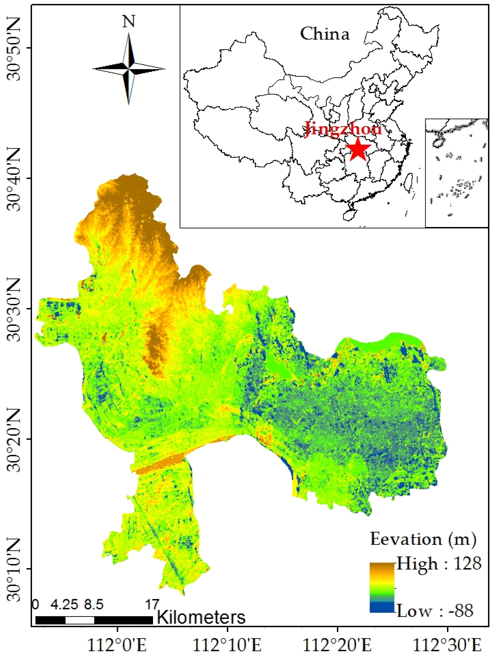
Jingzhou City is located in the south-central part of Hubei Province; the middle reaches the Yangtze River. The city lies adjacent to Wuhan in the east, Yichang in the west, Changde in the south and Jingmen and Xiangyang in the north (Figure 1). Jingzhou City has an abundant amount of precipitation as it has a subtropical monsoon climate. With a relative altitude ranges from 20 cm–50 cm, the plain area accounts for the highest proportion. Due to the strategies of the middle-part and Yangtze River Delta zone developments, as well as the improvement of the investment environment, Jingzhou City has witnessed a rapid urban sprawl in recent years. All of these have made a dramatic impact on the ecological environment and basic farmland in the suburban areas of Jingzhou City.
2.2. Data Source and Pretreatment
The images were of high quality and lacked a cloud layer, and they were qualified for land surface temperature retrieval. The data sources of images are shown in Table 1.
The pretreatment of the remote sensing images consisted of geometric correction and cloud removing. For geometric correction, the remote sensing images are projected onto a horizontal plane to conform to the map projection system. Geographic referencing is the process of assigning coordinates to the map. Combined with Gauss–Kruger projection and second-order polynomial curve fitting, the nearest neighbor algorithm was used for resampling under the GIS software on a 1:50,000-scale map. To perform a precise geometric correction of the remote sensing images, the obtained ETM+, TM and OLI_TIRS images were subjected to Gauss–Kruger/Krasovsky projection [33].
2.3. Method
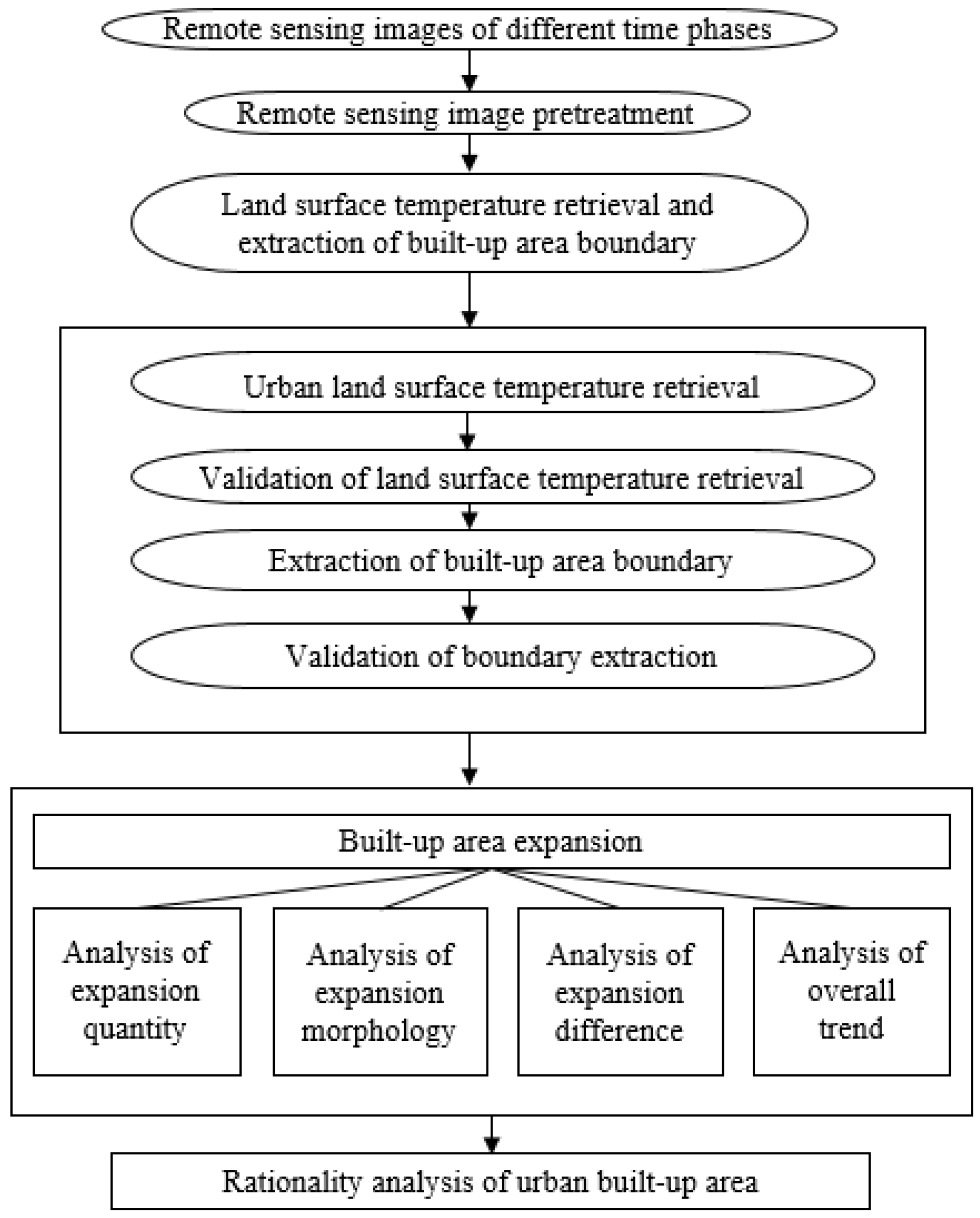
The basic principle was to use the Landsat TM/ETM+/OLI_TIRS images to extract the boundaries of urban built-up areas in different periods. Then, the temporal-spatial characteristics of urban built-up area expansion of Jingzhou in the past 15 years were analyzed. The conceptual and theoretical framework of the study is shown in Figure 2.
2.4. Extraction of Urban Built-Up Area Boundary
2.4.1. Rationale of Land Surface Temperature Retrieval
The mono-window algorithm was used to retrieve the land surface temperature due to its high precision. This algorithm proposed by Qin et al. [19] is based on heat conduction equation and requires no atmospheric correction. The atmosphere can be divided into several parallel, but distinct layers on a clear day without an obvious vertical atmospheric vortex. The real-time ground meteorological data (e.g., air temperature and atmospheric water content) can be combined with the standard atmospheric data, even in the absence of real-time atmospheric profiles. This algorithm has the following equation [19,20]:
where Ts is land surface temperature (K); Ta is mean atmospheric temperature (K); a and b are constants (see Table 2); C and D are intermediate variables, with C = ετ and D = (1 − τ) ([1 + (1 − ε) τ]; ε is ground emissivity; τ is atmospheric transmittance; TTIB (TIB is the thermal infrared bans which include band 6 of TM, band 6H of ETM+ and band 10 of TIRS) is the brightness temperature of the pixels (K) detected by the sensor at the satellite altitude, and it represents the changes of surface thermal radiation and surface temperature. Band 6H of ETM+ is high gain state data with slightly high sensitivity to inverse brightness temperature than the low gain state.
Ts = [a × (1 − C − D) + (b × (1 − C − D)) + C + D] × TTIB − D × Ta]/C
2.4.2. Calculation of Brightness Temperature
The pixel temperature can be directly obtained by Planck radiation [19,20,34] or the equation below:
where K1 and K2 are the band-specific thermal conversion constants for thermal infrared band.
TTIB = K2/ln(1 + K1/L(λ))
For the Landsat 5 images (TM) and Landsat 7 images (ETM+), the spectral radiance computed from the DN value has the following relation with its DN value [34]:
L(λ) = Grescale × QDN + Brescale
In the formula, L(λ) is the spectral radiance (W·m−2·sr−1·μm−1) of the thermal infrared band. QDN refers to the original DN value, 0 ≤ QDN ≤ 255. Grescale refers to the band-specific rescaling gain factor (W·m−2·sr−1·μm−1/QDN). Brescale refers to the band-specific rescaling bias factor (W·m−2·sr−1·μm−1).
For Landsat 8 images (TIRS), the spectral radiance computed from the DN value has the following relation with its DN value [22]:
L(λ) = MLQDN + AL
In the formula, ML (W·m−2·sr−1·μm−1/QDN) is the band-specific multiplicative rescaling factor from the metadata (RADIANCE_MULT_BAND_x, where x is the band number), and AL (W·m−2·sr−1·μm−1) is the band-specific additive rescaling factor from the metadata (RADIANCE_ADD_BAND_x, where x is the band number). The constants for computing brightness temperature are shown in Table 3.
2.4.3. Calculation of Atmospheric Transmittance
The Atmospheric Correction Parameter Calculator at http://atmcorr.gsfc.nasa.gov/ can be used to calculate the atmospheric transmittance. Besides the year 2000, the values of atmospheric transmittance after 2004 (2004, 2010 and 2014) were obtained as 0.89, 0.31 and 0.88, respectively.
According to Qin et al. [20], the values of atmospheric transmittance before 2000 can be calculated from the atmospheric water content and air temperature. We used the 1999 remote sensing images to perform atmosphere simulation (ENVI FLAASH). The results show that the average atmospheric water content is 4.0492 g/cm−2, and the region of interest has a mid-latitude summer climate. Based on Table 4, the atmospheric transmittance is 0.48.
2.4.4. Calculation of Mean Atmospheric Temperature
Using the air temperature data provided by the Jingzhou weather station, the surface air temperatures T0 (2 m) at 10:55 a.m. on 10 September 1999, 10:41 a.m. on 8 April 2004, 10:52 a.m. on 30 July 2010 and 11:02 a.m. on 6 May 2014 were estimated as 30.5 °C, 20.3 °C, 35.3 °C and 26.3 °C, respectively. The annual mean atmospheric temperatures (Ta) in each year were then estimated as 297.254666 K, 287.807324 K, 301.700474 K and 293.36159 K, respectively, by using the mean atmospheric temperature equation for the mid-latitude summer climate.
The mean atmospheric temperature equation for the mid-latitude summer climate is written as [20]:
Ta = 16.0110 + 0.92621 × T0
2.4.5. Calculation of Ground Emissivity
For Landsat 5 Images and Landsat 7 Images
Combined with the algorithm proposed by Qin [20], the parameter values were assigned using the equation proposed by Sobrino et al. [27]. Thus, for water bodies, εw = 0.995; for bare soil, εs = 0.972; and for vegetation, εv = 0.986. Table 5 presents the ground emissivity equations for different land cover types.
The mixed surfaces are composed by bare soil and vegetation with different vegetation covers and different values of soil and vegetation emissivities. Pv is vegetation cover, estimated by:
PV = [(NDVI − NDVIS)/(NDVIV − NDVIS)]2
NDVIW, NDVIV and NDVIS are the corresponding mean NDVI value of the water body, vegetation and bare soil, which are extracted by supervised classification on the remote sensing image processing platform. NDVI is the Normalized Difference Vegetation Index, and p3 and p4 represent the NDVI value of red band and near-infrared band respectively. NDVI is estimated by:
NDVI = (p4 − p3)/(p4 + p3)
For Landsat 8 Images
Combined with the algorithm proposed by Wang et al. [22], the parameter values were assigned using the equation proposed by Sobrino et al. [38]. Thus, for water bodies, εw = 0.991; for bare soil, εs = 0.966. Table 6 presents the ground emissivity equations for different land cover types.
Subject to:
where C is a term due to surface roughness and F′ is a geometrical factor ranging between zero and one.
Cλ = (1 − 0.966) × 0.973 × F′(1 − PV)
PV is estimated by:
PV = [(NDVI − NDVIS)/(NDVIV − NDVIS)]2
NDVIW, NDVIV and NDVIS are the corresponding mean NDVI value of the water body, vegetation and bare soil, which are extracted by supervised classification on the remote sensing image processing platform. The p4 and p5 represent the NDVI value of red band and near-infrared band respectively. NDVI is estimated by:
NDVI = (p5 ‒ p4)/(p4 + p5)
3. Results
3.1. Results of Land Surface Temperature Retrieval
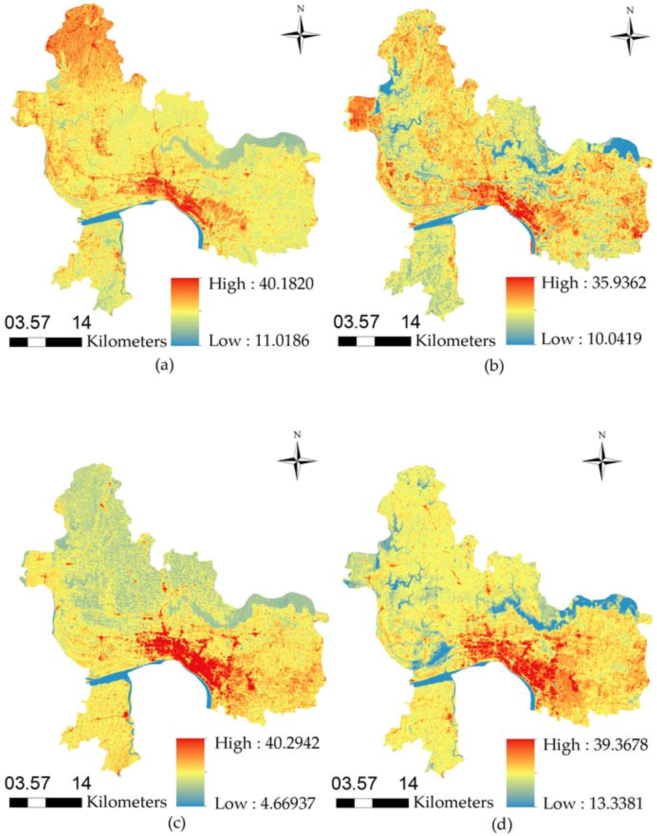
The land surface temperatures of Jingzhou City were retrieved in the thermal infrared band for the years 1999, 2004, 2010 and 2014 by using the above of brightness temperature, atmospheric transmittance and ground emissivity equations. Figure 3 shows the results.
It can be seen from the above figures that in Jingzhou city, the vegetation (green regions and part of the blue regions) follow the water bodies (blue regions and part of the green regions) as having the lowest temperature. Farmland temperatures are higher than vegetation (yellow regions and part of the green regions). Urban land surface temperature is much higher than the temperature of the suburban areas (red regions), and this is the so-called urban heat island. Thus, the temperature varies considerably for different types of underlying surfaces; the water bodies have the lowest temperatures, followed by the underlying surfaces in the suburban areas (forest land, grassland and farmland); the underlying surfaces of the urban built-up areas have the highest temperatures, including the urban construction and industrial lands. Comparison of the air temperatures at the time of satellite passing during the four years indicates that the underlying surfaces of the urban built-up areas always have the highest temperature. Thus, the underlying surfaces of the urban built-up areas and suburban areas will be higher than the air temperature during the daytime. The thermal properties of the underlying surfaces, vegetation cover and soil humidity can be used to explain this difference. Generally, the underlying surfaces of the urban built-up areas have a smaller reflectance than suburban areas. This means the underlying surfaces of the urban built-up areas absorb a greater amount of solar radiation. Impervious materials usually make up the road surface, which allows less heat to escape. Moreover, the rough surface and low vegetation cover in the urban built-up areas also cause an increase in temperature of the underlying surfaces, as compared with the farmland and water bodies. Suburban areas are generally covered by forestland, farmland and grassland, whose thermal capacity, thermal conductivity and thermal inertia are all smaller than those of the urban built-up areas. However, the soil water content and vegetation cover of the suburban areas are much higher than those of the urban built-up areas. This is the reason why the ground temperature of the suburban areas is much lower than that of the urban built-up areas. Water bodies have higher specific heat and thermal inertia, and therefore, the temperature increases more slowly and the surface temperature distributes more uniformly. During the daytime, water bodies have a lower temperature than the underlying surfaces of the urban built-up areas and suburban areas.
3.2. Urban Built-Up Area Boundary Extraction
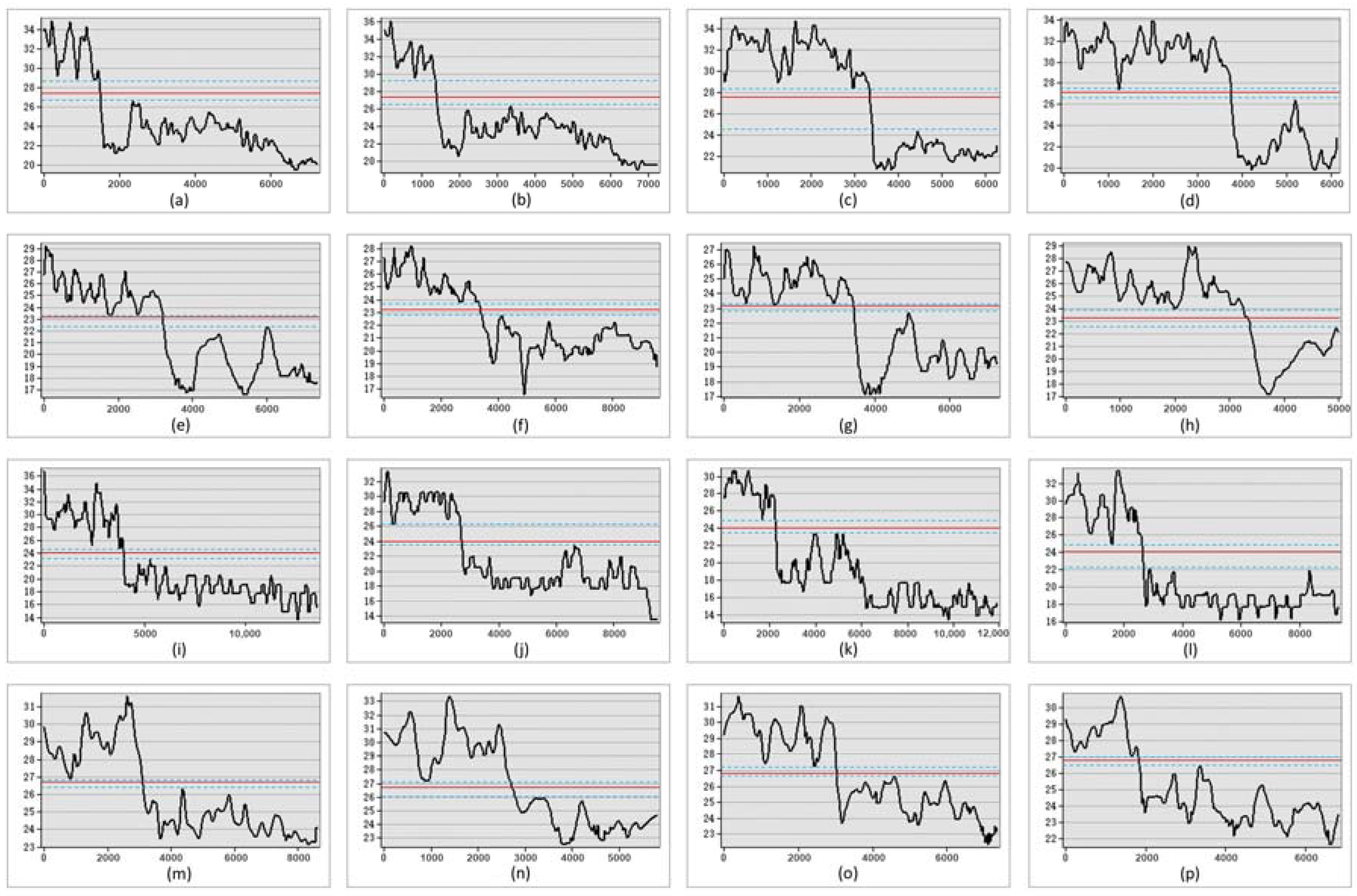
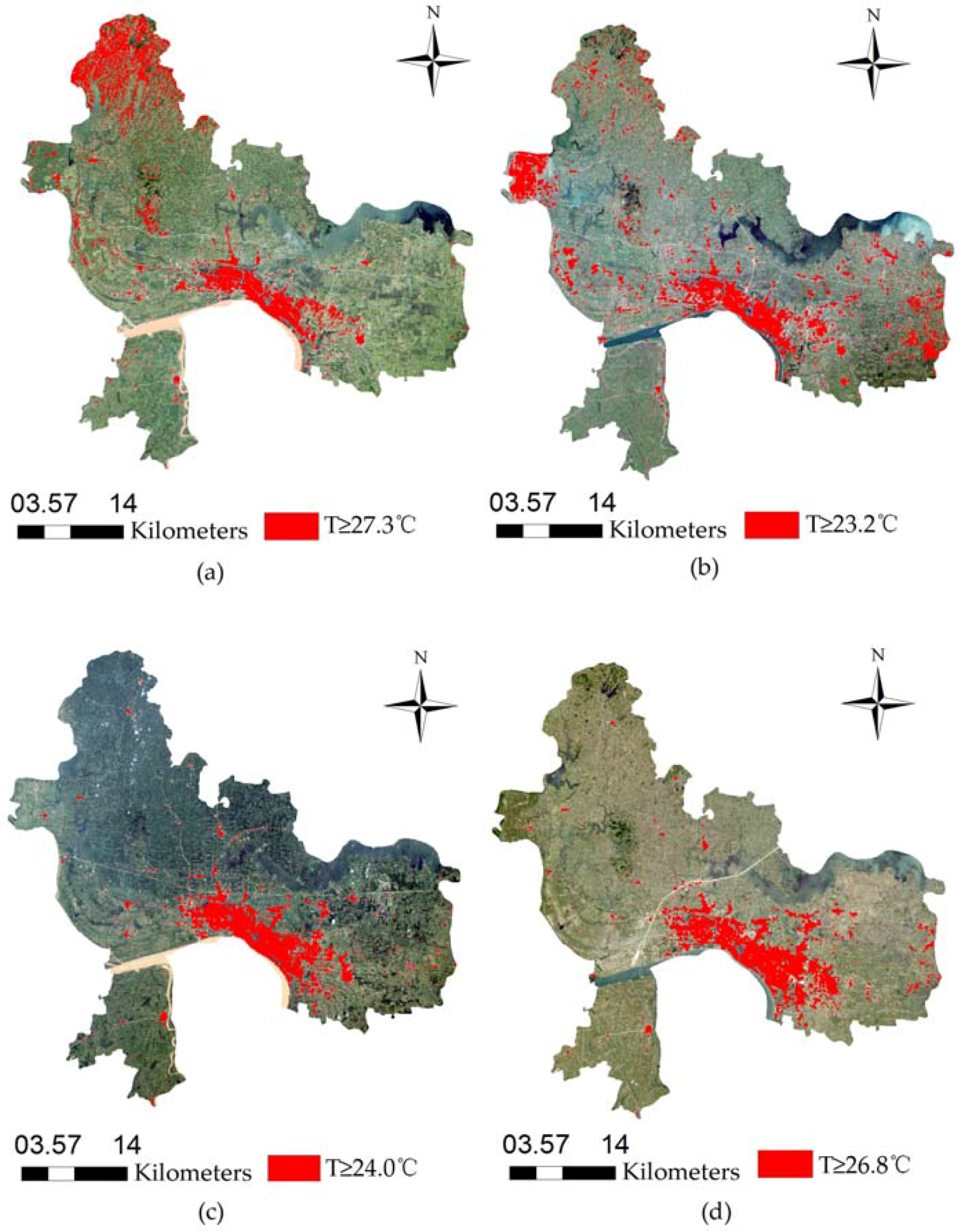
We drew four interpolated lines from high temperature areas to low temperature areas on the images of land surface temperature in the four years, respectively (Figure 4). The data of interpolated lines were then analyzed, and the temperature value of the lowest total frequency and maximum total frequency difference with the adjacent temperature value is extracted in each set of data. We found that these temperature values were concentrated within the two blue lines of the figure and only appeared outside once. We can conclude that these are the temperature threshold’s range of the urban built-up area boundary. After averaging these temperature values for each year, the temperature threshold of four years can be obtained. The temperature thresholds for discriminating the urban built-up areas in 1999, 2004, 2010 and 2014 were set to be 27.3 °C, 23.2 °C, 24 °C and 26.8 °C, respectively. The regions above the threshold values were extracted as the urban built-up areas. The boundaries extracted for the four time phases are shown below.
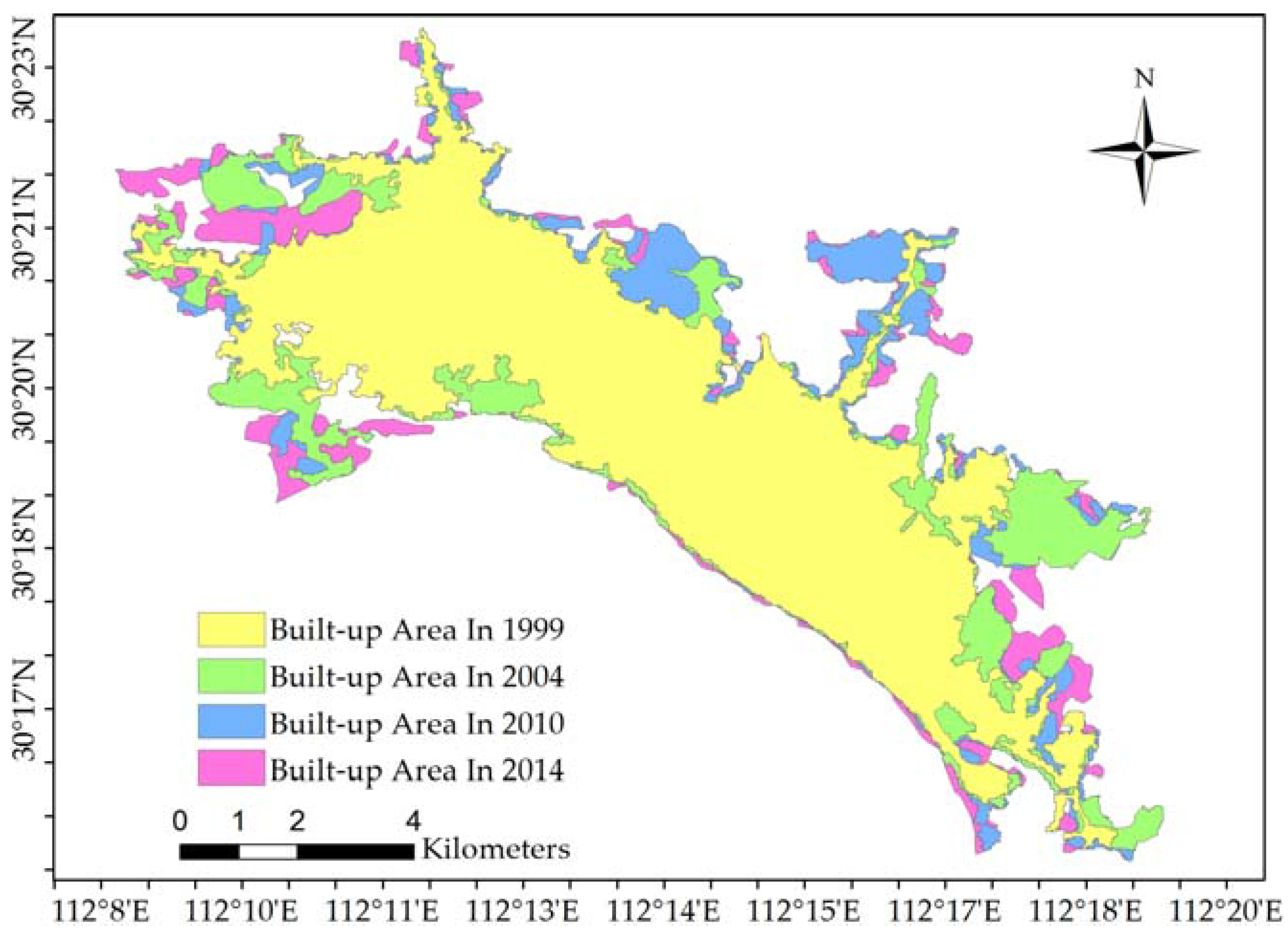
The extracted regions (red color) in the four maps basically coincide with the existing urban built-up areas (Figure 5). From 1999–2014, the areas in red continue to expand, indicating a constant increase of the urban built-up areas in the past 15 years. This is what we call the urban sprawl. The lakes and greening areas in the urban built-up areas have a lower temperature and therefore are not shown in red. Since the Jingzhou Industrial Park on Oriental Avenue is not yet connected to the previously built-up area, it is removed from the map. Then, GIS software was used to process the small red patches, and image fusion was completed to obtain the built-up area boundaries during the four years (Figure 6).
4. Discussion
4.1. Overall Trend of Built-Up Area Expansion of Jingzhou
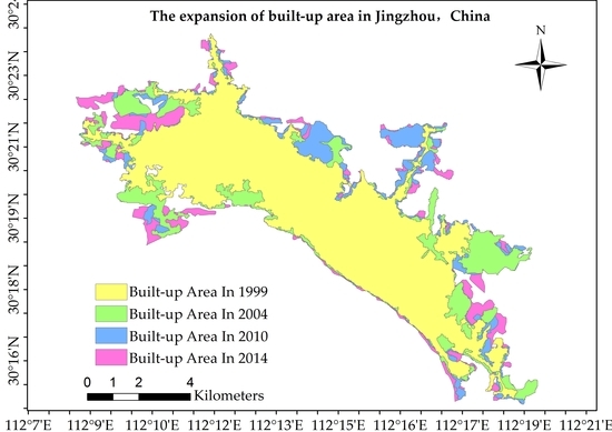
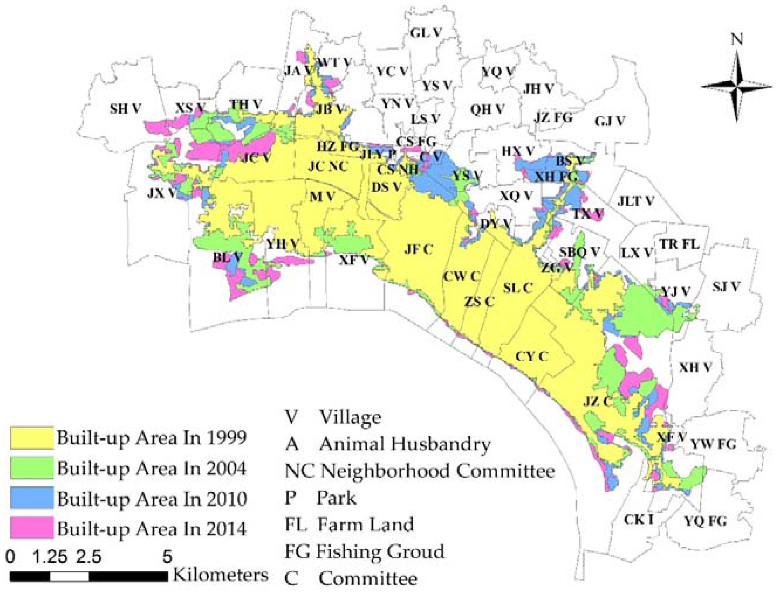
The built-up area boundaries were extracted from the pretreated remote sensing images of the four time phases, along with the size of the built-up areas during each year. First, GIS was used for superposition of the images, and the distribution of the built-up area expansion in the Jingzhou and Shashi District of Jingzhou City was analyzed. Figure 7 shows the processed map, which indicates a constant increase of the scale of the built-up areas in both the Jingzhou and Shashi District of Jingzhou City from 1999–2014. The built-up area of 1999 is used as the center for both districts, though the intensity of expansion varies in different directions, and the expansion is most intensive in the axial direction.
In 1999, the built-up area in Jingzhou City was 50.243 km2, and all of the area was distributed between the Jingcheng District, Chongwen District community (CW C), Zhongshan Road community (ZS C), Shengli Road community (SL L), Chaoyang road community (CY C), and Jingzhou Development Zone. In 2004, the built-up area of Jingzhou had increased 11.035 km2 from 1999 to 61.278 km2. In the Jingzhou District, the northward expansion towards the Xinsheng Village (XS V), Taihui Village (TH V) and Jing’an Village (JA V) makes the greatest contribution. For the Shashi District, the built-up area expansion is mainly contributed by the northward, east-northward and south-eastward expansion of Jingzhou Development Zone. In 2010, the built-up area in Jingzhou had increased 5.264 km2 from 2004 to 66.542 km2. The new built-up areas in the Jingzhou District appeared in the periphery of the built-up areas of 2004. They were mainly concentrated in the Jingcheng Village (JC V), Xinsheng Village (XS V), Taihui Village (TH V) and Bailong Village (BL V). In addition to further enlargement of Jingzhou Development Zone, the expansion from Jiefang Road Community (JF C) to the Sanbanqiao Village (SBQ) and from the Shengli Road community (SL C) to the Tongxin (TX V) and Baishuo (BS V) villages made the greatest contribution for the Shashi District. In 2014, the built-up area of Jingzhou reached up to 73.898 km2. From 2010–2014, the new built-up areas in Jingzhou District were mainly concentrated in the Jingcheng Village (JC V), Xinsheng Village (XS V), Taihui Village (TH V), Bailong Village (BL V) and Sanhong Village (SH V). The new built-up areas in the Shashi District were mainly concentrated in the Jingzhou Development Zone, with a mild expansion from the Shengli Road community (SL C) to the Tongxin Village (TX V).
4.2. Spatial and Temporal Characteristics of Built-Up Area Expansion of Jingzhou
4.2.1. Expansion Quantity
We further extracted the size of the built-up area in the four years based on the extracted boundaries of Jingzhou urban built-up areas, which are 50.243 km2, 61.278 km2, 66.542 km2 and 73.898 km2, respectively. The percentage of the urban expansion are 4.393% (1999–2004), 1.432% (2004–2010) and 2.764% (2010–2014). The trend of urban built-up area expansion of Jingzhou was analyzed (Table 7 and Table 8).
4.2.2. Index Calculation
Compactness Index
The compactness index is an important index to measure the spatial morphological change of urban built-up area [39] (see Equation (15)).
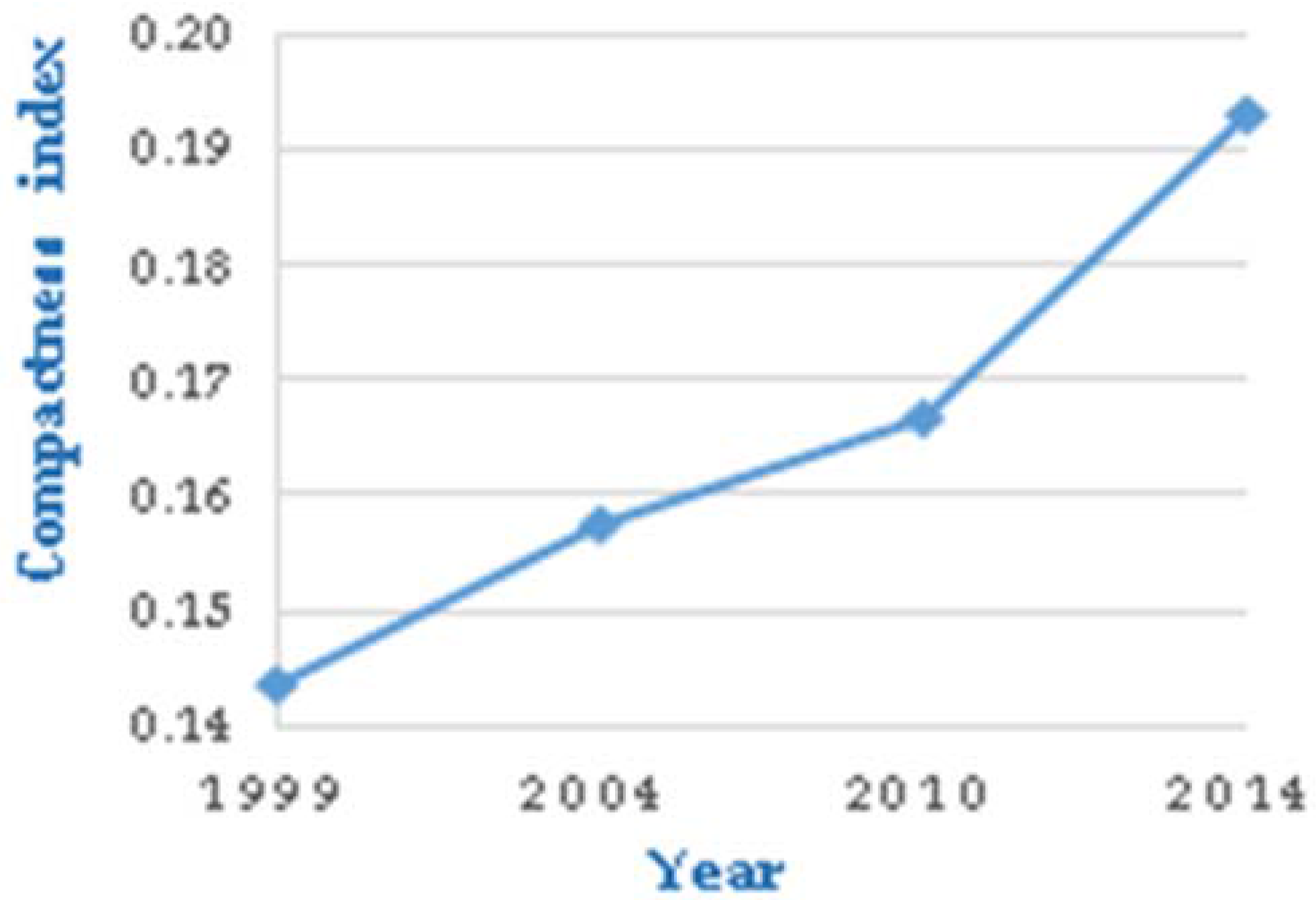
In the equation, J is the compact degree of urban built-up area, S is the area of urban built-up area and Z is the perimeter of urban built-up area. If the shape of the urban built-up area is close to circular, the compact index will be close to one, and the urban space is more compact. On the contrary, if the compact index is far from one, the urban space is less compact. As shown in Table 8 and Figure 8, from 1999–2014, the compactness index of the built-up area remains low, but a gradual increasing trend is shown. Therefore, the morphology becomes simpler as the urban spatial compactness increases.
Fractal Dimension
The spatial fractal dimension can be used to describe the complexity of urban boundary shape and show the change of land use shape [40]. The fractal dimension of urban spatial shape can be defined as:
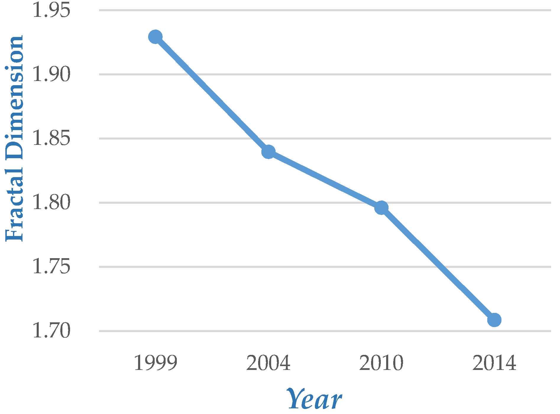
In the equation, F represents the fractal dimension of urban patches in a certain period, and S and Z are the area and circumference of the patches in the urban built-up area in a certain period. The closer the geometry is to the circle, the smaller is the fractal dimension, otherwise it is bigger. In the above table, the fractal dimension from 1999–2014 is far from being one, indicating a complicated spatial form of Jingzhou’s built-up area. In Figure 9, the fractal dimension of 1999 is the largest (1.9293), and that of 2014 is the smallest (1.7085). The fractal dimension decreases every year from 1999–2014. Apparently, internal restructuring is the dominating trend in Jingzhou’s urban development over the past 15 years.
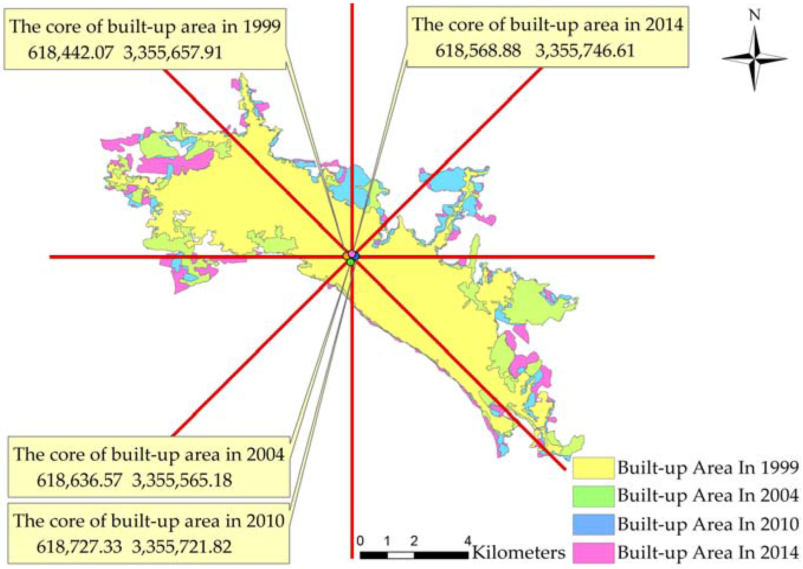
Barycenter Index of the Built-Up Area
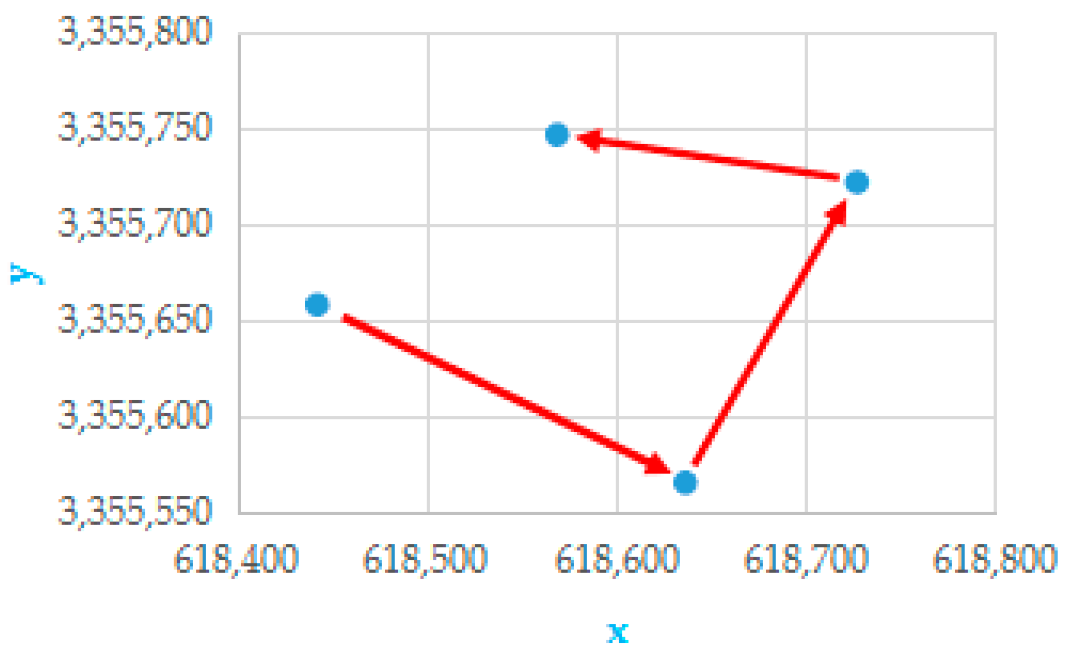
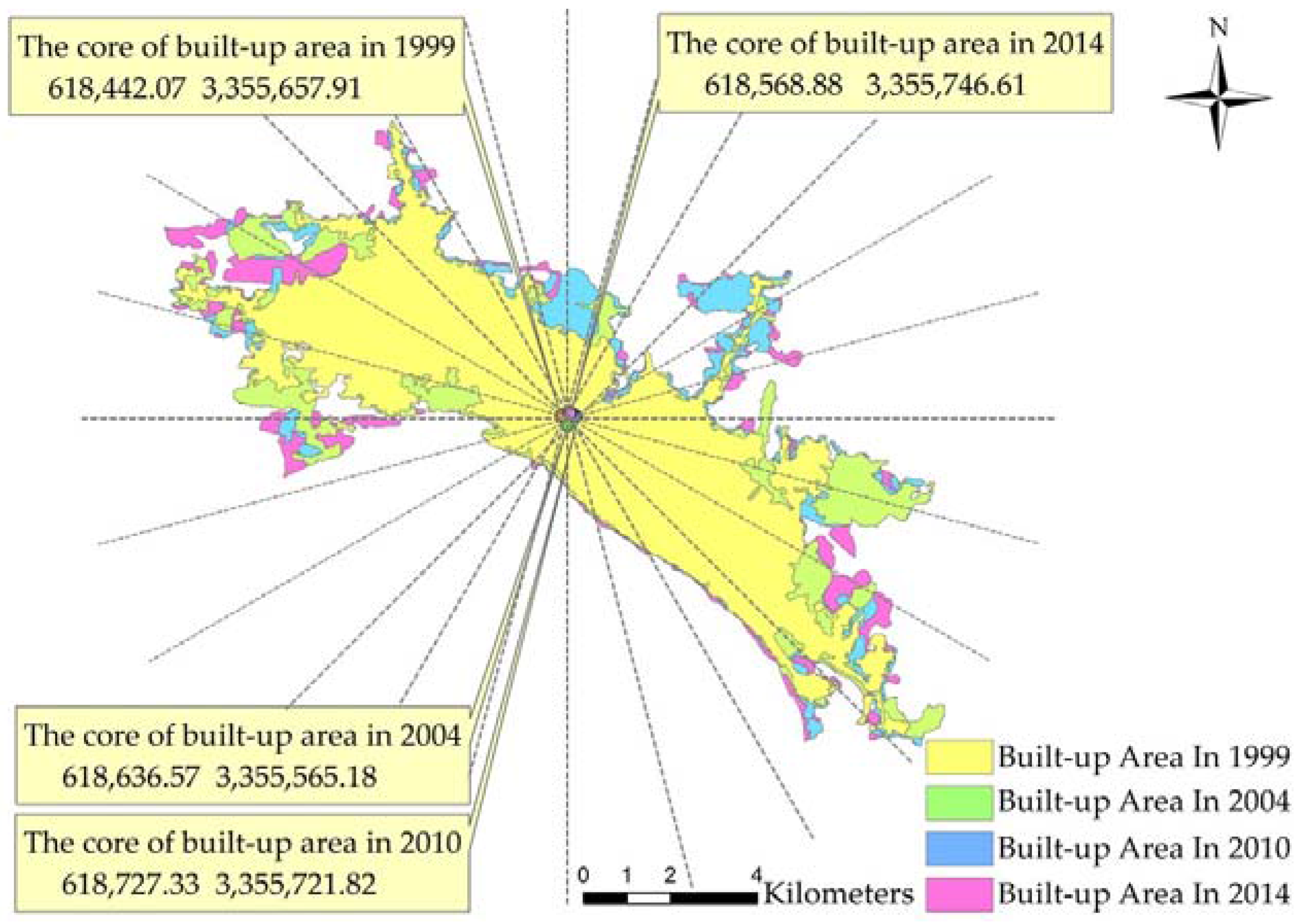
The barycenter index can be used to describe urban spatial distribution. The barycenter of the built-up area is the equilibrium point of the city’s uniform distribution. It can be obtained by computing weighted average of the geometric center coordinates of each urban plot. Using the GIS software, we calculated the coordinates of the barycenter for each year based on the geometric shape of the built-up area (see the Figure 10). The map portrays the location of the barycenter of the built-up area. In Figure 10, we observe that the barycenter of the built-up area barely shifts from 1999–2014. This means that spatial extension is the primary form of urban expansion in Jingzhou.
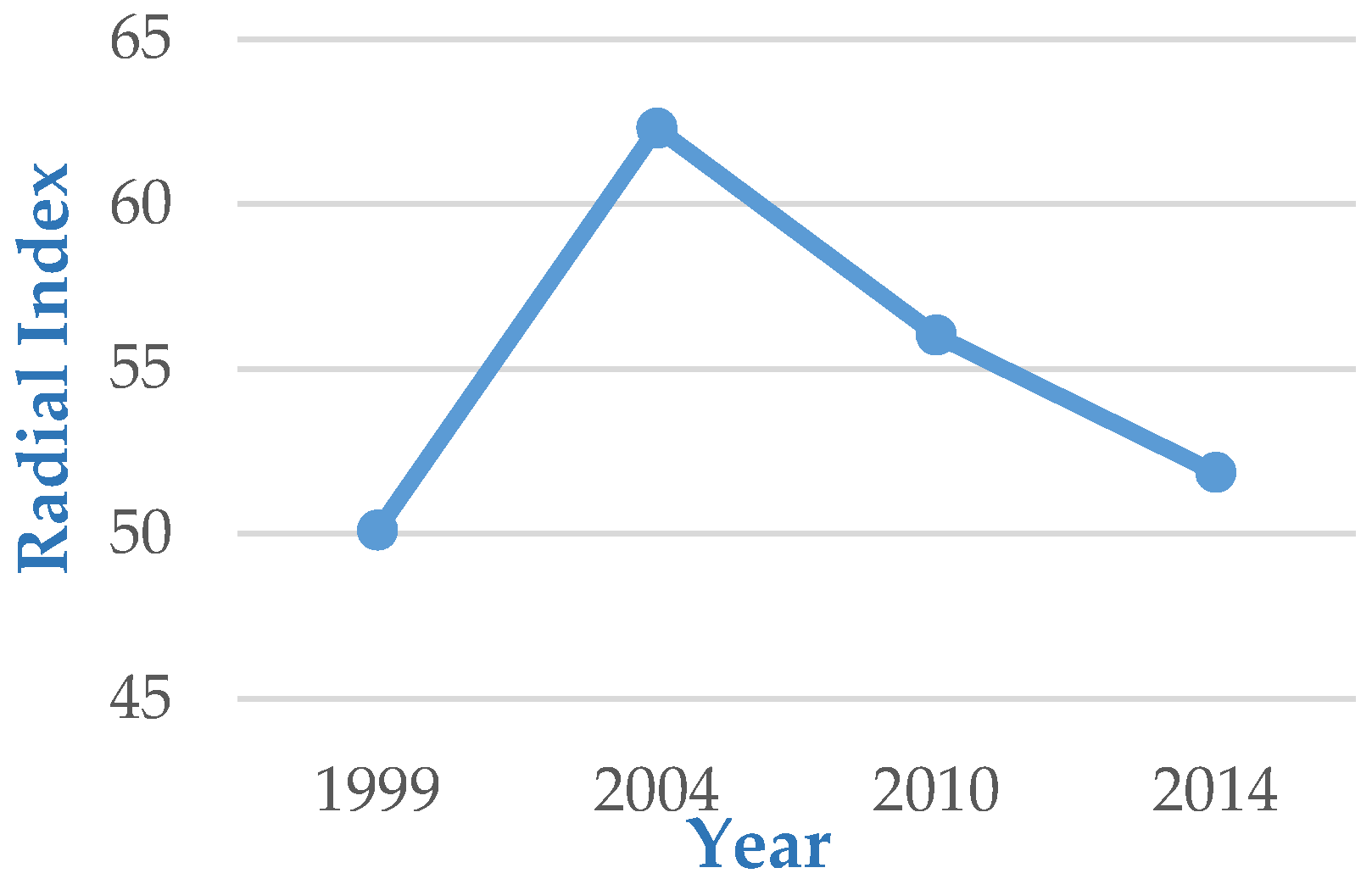
Radial Index
The radial index, also known as the Boyce–Clark shape index, was first proposed by Boyce and Clark [39]. By using each year’s barycenter of the built-up area as the core, 24 radial lines are drawn from the core. The inclusion angle between the two adjacent lines is 15° (Figure 11). As shown in Figure 12, the radial indices of the built-up area from 1999–2014 were calculated. It is found that the radial index is generally high, indicating spatial form irregularity of Jingzhou’s built-up area. The radial index increases from 1999–2004, indicating the growing spatial form irregularity. After 2004, the radial index consistently decreases, indicating the increasing spatial form regularity of Jingzhou’s built-up area.
Difference of Spatial Extent of Built-Up Area Expansion
By taking the position with average coordinates of the barycenter over four years as the center, eight directions of built-up area expansion were drawn up. The calculation equation [41] is:
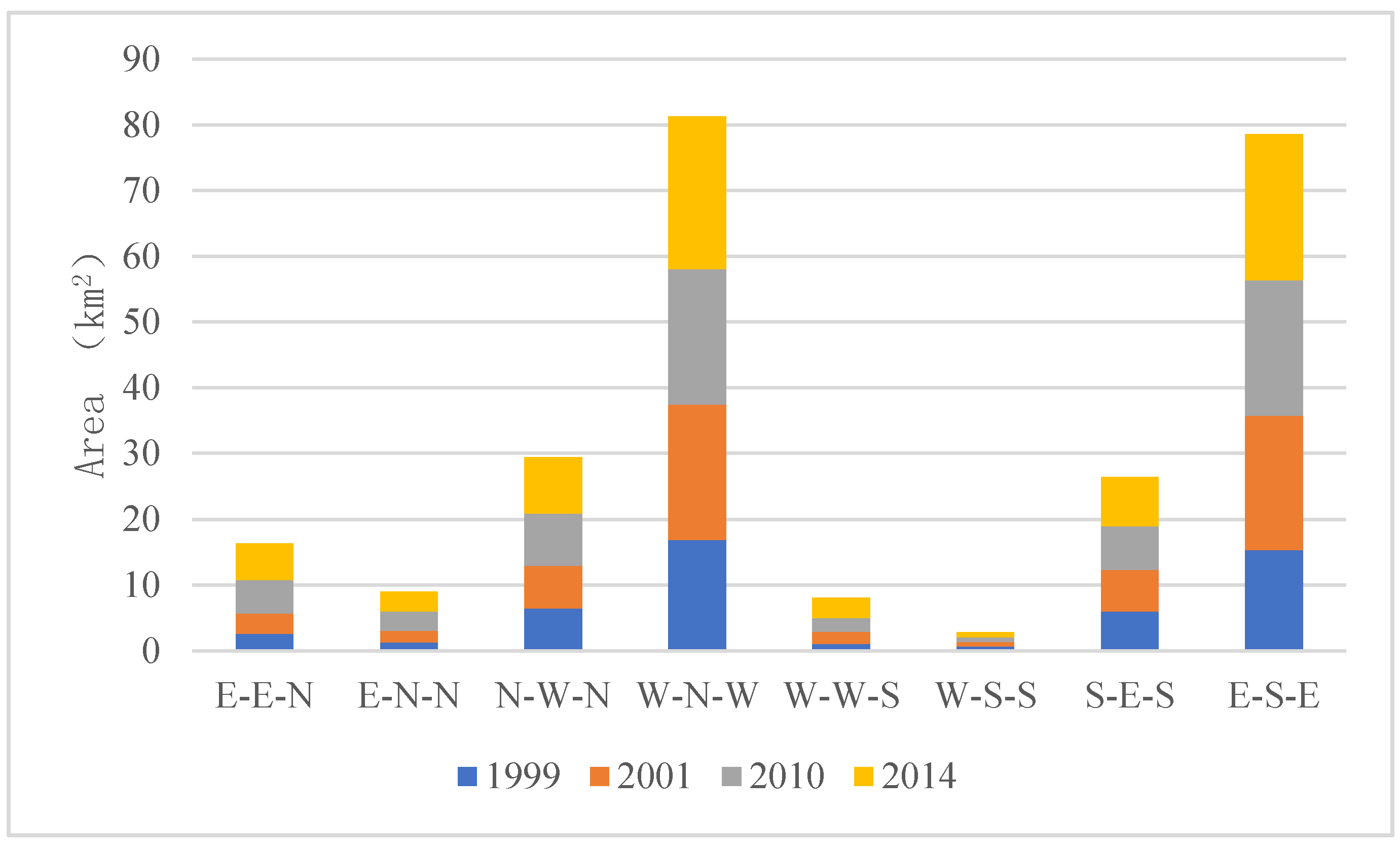
The SBC, ri and n in the upper equation represent the radial index, the radius of a graph center to the periphery of the graph and the number of radiation radii with the same angle difference. Then, the built-up area at two different positions in each of the eight directions (Figure 13) during each period was calculated by using the GIS software. Thus, the standard deviations for each year were obtained, as shown in Table 8.
It can be seen from Table 9 that throughout 1999–2014, the urban built-up area increases in different directions. The land surface temperature retrieval is affected to some degree by cloud removal, leading to an underestimation in the west-south-south direction in 2010 and 2011; when compared with the former year, the built-up are is smaller, but within a range of allowable error. The change of standard deviation of the built-up area from 1999–2014 indicates the spatial expansion in eight directions, and the difference in area increments in the different directions continues to accumulate over time. As shown in the figure below, from 1999–2014, the spatial extent of the built-up area differs significantly in each direction, especially in the east-south-east direction and the west-north-west direction (Figure 14).
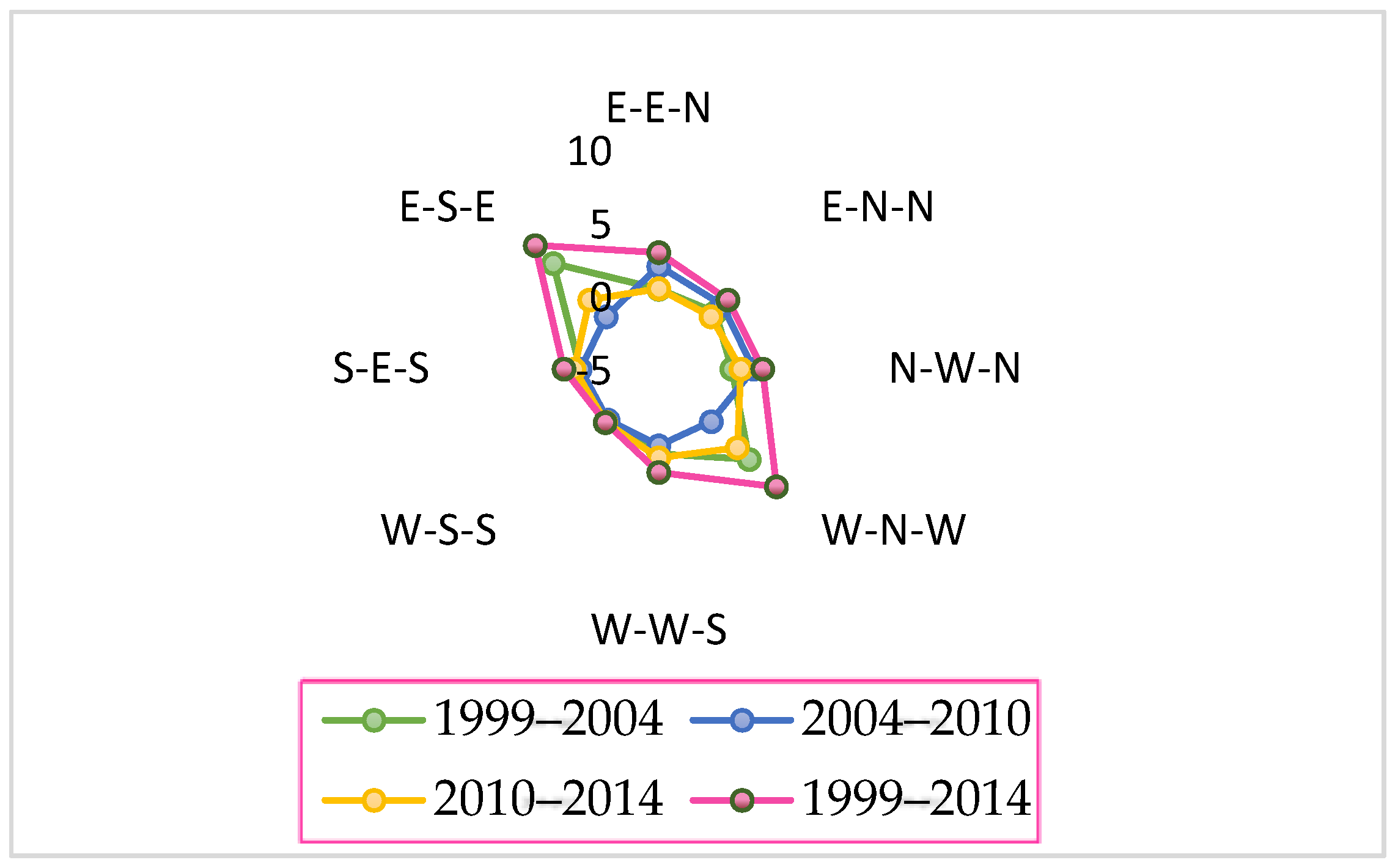
According to Table 10 and Figure 15, the expansion is fastest in the east-south-east direction from 1999–2004, followed by that in the west-north-west direction. From 2004–2010, the expansion is the fastest in the east-east-north direction, followed by that in the east-north-north direction. The expansion rate first decreases, then increases, and slows down from 2004–2010. The standard deviation is the smallest from 2004–2010, indicating the smallest difference in the expansion rate of the built-up area in the eight directions. In the last column, the total expansion quantity is the highest in the east-south-east direction from 1999–2014, and it is the lowest in the west-south-south direction.
4.3. Rationality Evaluation of the Built-Up Area Expansion of Jingzhou City
4.3.1. Urban Area-Population Elasticity Coefficient
The urban area-population elasticity coefficient can be used to describe the relationship between urban expansion speed and urban population growth rate [42]. The calculation equation is:
R(i) = S(i)/Pop(i)
R(i), Pop(i) and S(i) respectively represent the expansion elastic coefficient of the built-up area, the average growth rate of the urban population and the average growth rate of the built-up area during the i period. The urban area used for the evaluation was the built-up area retrieved from the remote sensing images. The China City Statistical Yearbook was referenced for the urban population. Equation (17) was used to calculate the expansion elasticity index of Jingzhou’s built-up area from 1999–2014 (see Table 11).
Through a comprehensive analysis of the urbanization process in China, scholars believe that a reasonable value of R(i) is 1.12 (if urban population increases by 1%, the area of built-up area should increase by 1.12% [42]). If R(i) < 1.12, urban construction land will be in short supply; if R(i) > 1.12, the efficiency of land use is low. According to the above table, the urban area-population elasticity coefficients of Jingzhou City are all above the empirical value of 1.12. The built-up area continues expanding even with a negative population growth, especially during the years 2010–2014, indicating that the expansion rate of Jingzhou’s built-up area is much faster than the population growth rate.
4.3.2. Allometric Growth Model
The spatial and temporal evolution of urban and urban systems will obey the law of hetero-velocity growth in some sense [43]. The calculation equation is:
A represents the area of the built-up area; a is the proportional coefficient; and b is the scaling factor. P stands for urban population, and t stands for the year. The scaling factor b indicates the different growth relation of different speeds [43]: when b = 0.9, the urban area and urban population are growing at a same growth rate, and their growth rate is more appropriate; when b < 0.9, the growth is negative, and the growth of the urban area is slower than the urban population; when b > 0.9, the growth is positive, and the growth of the urban area is expanding faster than the urban population.
A = aPtb
By using statistical software, the allometric growth model was derived based on the built-up area of Jingzhou in the Jingzhou Statistical Yearbook (1999–2014) and the urban population of Jingzhou in the China City Statistical Yearbook (1999–2014):
At = 3.166 × 10⁻⁵Pt3.072
The goodness-of-fit is 0.403, and it passes the significance test at the 0.01 level. The scaling factor b = 3.072, which is above the empirical value of 0.9. Hence, the rate of spatial expansion of Jingzhou’s built-up area is greater than the population growth rate. This means the urban sprawl is unreasonably fast for the urban population growth of Jingzhou.
5. Conclusions
- (1)
- Based on land surface temperature retrieval from the remote sensing images, this study established the procedures for extracting the built-up area boundary of Jingzhou. The Landsat 5, 7 and 8 images were chosen as the data sources by considering the features of the study area, research goals, requirements on remote sensing images for retrieval and availability of the remote sensing images. After pretreatment, the land surface temperature maps of Jingzhou in different years were calculated by using the mono-window algorithm. The threshold method was used to extract the built-up area from the remote sensing images.
- (2)
- Urban sprawl of Jingzhou uses the 1999 built-up area as the core, and the expansion rate differs in different directions. The expansion is the fastest along the axial direction. The expansion quantity and expansion rate both increase initially, then decrease. The development trend of the expansion speed is extra high-speed (urban expansion intensity >1.92) and high-speed (1.05 < urban expansion intensity < 1.92) and then extra high-speed. With a gradual improvement of the urbanization level, the intensity of the expansion initially increases, then decreases. There seems to be a trend of growing compactness over time for the spatial form of the built-up area, with the contour of the built-up area becoming increasingly regular. From 1999–2014, the spatial form of the built-up area evolves towards a more compact and orderly state. The barycenter of the built-up area barely shifts over time, indicating that extension from the initial site of the built-up area is the dominant form of expansion. However, over the past 15 years, the spatial extent of the built-up area has significantly differed in different directions. The expansion is the fastest in the east-south-east direction, followed by that in the west-north-west direction; the expansion in the west-south-south direction is the slowest.
- (3)
- According to the calculation of the urban area-population elasticity coefficient, the urban sprawl of Jingzhou is much faster than the population growth rate. The algometric growth model has proven this. In conclusion, the expansion of Jingzhou’s built-up area is too fast for the local population growth.
The urban built-up area boundary extraction, based on land surface temperature retrieval, can be applied to most cities that have a significant urban heat island effect and be helpful for carrying out macro-control and management of land resources. However, there are some cities that have a cold island effect. Future research will focus on the urban built-up area boundary extraction of types of cities and improving the precision of land surface temperature inversion and the setting of temperature thresholds of the urban built-up boundary.
Acknowledgments
This work was supported by the National Natural Science Foundation of China (71673258). Landsat 5, 7 and 8 images are available from the U.S. Geological Survey. We would also thank the Editor and the anonymous reviewers for their insightful suggestions and comments.
Author Contributions
Lin Wang designed and conducted the experiments and wrote the manuscript. Jianghong Zhu and Yanqing Xu provided suggestions for the data analysis and manuscript writing. Zhanqi Wang revised the manuscript and assumed the foundational responsibility. All co-authors have contributed to the group discussions on the analysis, results and to the final draft.
Conflicts of Interest
The authors declare no conflict of interest.
References
- Jensen, J.R.; Toll, D.L. Detecting residential land-use development at the urban fringe. Photogramm. Eng. Remote Sens. 1982, 48, 629–643. [Google Scholar]
- Marquez, L.O.; Smith, N.C. A framework for linking urban form and air quality. Environ. Model. Softw. 1999, 14, 541–548. [Google Scholar] [CrossRef]
- Singh, A. Digital change detection techniques using remotely-sensed data. Int. J. Remote Sens. 1989, 10, 989–1003. [Google Scholar] [CrossRef]
- Masek, J.; Lindsay, F.; Goward, S. Dynamics of urban growth in the Washington DC metropolitan area, 1973–1996, from Landsat Observations. Int. J. Remote Sens. 2000, 21, 3473–3486. [Google Scholar] [CrossRef]
- Zha, Y.; Gao, J.; Zhang, Y. Grassland productivity in an alpine environment in response to climate change. Area 2005, 37, 332–340. [Google Scholar] [CrossRef]
- Huang, X.; Schneider, A.; Friedl, M.A. Mapping sub-pixel urban expansion in China using MODIS and DMSP/OLS nighttime lights. Remote Sens. Environ. 2016, 175, 92–108. [Google Scholar] [CrossRef]
- Jing, W.; Yang, Y.; Yue, X.; Zhao, X.D. Mapping Urban Areas with Integration of DMSP/OLS Nighttime Light and MODIS Data Using Machine Learning Techniques. Remote Sens. 2015, 7, 12419–12439. [Google Scholar] [CrossRef]
- Lu, D.; Tian, H.; Zhou, G.; Ge, H. Regional mapping of human settlements in southeastern China with multisensor remotely sensed data. Remote Sens. Environ. 2008, 112, 3668–3679. [Google Scholar] [CrossRef]
- Hall, P. The future of the metropolis and its form. Reg. Stud. 1997, 31, 211–220. [Google Scholar] [CrossRef]
- Bourne, L.S. Reurbanization, uneven urban development, and the debate on new urban forms. Urban Geogr. 1996, 17, 690–713. [Google Scholar] [CrossRef]
- Braimoh, A.K.; Onishi, T. Spatial determinants of urban land use change in Lagos, Nigeria. Land Use Policy 2007, 24, 502–515. [Google Scholar] [CrossRef]
- Kuang, W.; Liu, Y.; Dou, Y.; Chi, W.; Chen, G.; Gao, C.; Yang, T.; Liu, J.; Zhang, R. What are hot and what are not in an urban landscape: Quantifying and explaining the land surface temperature pattern in Beijing, China. Landsc. Ecol. 2015, 30, 357–373. [Google Scholar] [CrossRef]
- Wang, N.; Wu, H.; Nerry, F.; Li, C.; Li, Z.-L. Temperature and emissivity retrievals from hyperspectral thermal infrared data using linear spectral emissivity constraint. IEEE Trans. Geosci. Remote Sens. 2011, 49, 1291–1303. [Google Scholar] [CrossRef]
- Zhang, Y.; Chen, L.; Wang, Y.; Chen, L.; Yao, F.; Wu, P.; Wang, B.; Li, Y.; Zhou, T.; Zhang, T. Research on the contribution of urban land surface moisture to the alleviation effect of urban land surface heat based on Landsat 8 data. Remote Sens. 2015, 7, 10737–10762. [Google Scholar] [CrossRef]
- Li, Z.-L.; Tang, B.-H.; Wu, H.; Ren, H.; Yan, G.; Wan, Z.; Trigo, I.F.; Sobrino, J.A. Satellite-derived land surface temperature: Current status and perspectives. Remote Sens. Environ. 2013, 131, 14–37. [Google Scholar] [CrossRef]
- Wu, H.; Li, Z.L. Scale issues in remote sensing: A review on analysis, processing and modeling. Sensors (Basel) 2009, 9, 1768–1793. [Google Scholar] [CrossRef] [PubMed]
- Dewan, A.; Corner, R. Dhaka Megacity: Geospatial Perspectives on Urbanisation, Environment and Health; Springer: Berlin, Germany, 2014. [Google Scholar]
- Gilmore, S.; Saleem, A.; Dewan, A. Effectiveness of DOS (Dark-Object Subtraction) method and water index techniques to map wetlands in a rapidly urbanising megacity with Landsat 8 data. In Proceedings of the Research at Locate’15, Brisbane, Australia, 10–12 March 2015. [Google Scholar]
- Qin, Z.H.; Zhang, M.H.; Karnieli, A.; Berliner, P. Mono-window algorithm for retrieving land surface temperature from Landsat TM6 data. Acta Geogr. Sin. 2001, 56, 466–474. [Google Scholar]
- Qin, Z.; Karnieli, A.; Berliner, P. A mono-window algorithm for retrieving land surface temperature from Landsat TM data and its application to the Israel-Egypt border region. Int. J. Remote Sens. 2001, 22, 3719–3746. [Google Scholar] [CrossRef]
- Wan, Z.; Li, Z.L. A physics-based algorithm for retrieving land-surface emissivity and temperature from EOS/MODIS data. IEEE Trans. Geosci. Remote Sens. 1997, 35, 980–996. [Google Scholar]
- Wang, F.; Qin, Z.; Song, C.; Tu, L.; Karnieli, A.; Zhao, S. An improved mono-window algorithm for land surface temperature retrieval from Landsat 8 thermal infrared sensor data. Remote Sens. 2015, 7, 4268–4289. [Google Scholar] [CrossRef]
- Jiménez-Muñoz, J.C.; Sobrino, J.A. A generalized single-channel method for retrieving land surface temperature from remote sensing data. J. Geophys. Res. Atmos. 2003, 108. [Google Scholar] [CrossRef]
- Sobrino, J.; Jimenezmunoz, J.; Verhoef, W. Canopy directional emissivity: Comparison between models. Remote Sens. Environ. 2005, 99, 304–314. [Google Scholar] [CrossRef]
- Zhang, R.; Tian, J.; Su, H.; Sun, X.; Chen, S.; Xia, J. Two improvements of an operational two-layer model for terrestrial surface heat flux retrieval. Sensors (Basel) 2008, 8, 6165–6187. [Google Scholar] [CrossRef] [PubMed]
- Zhang, Y.; Odeh, I.O.A.; Han, C. Bi-temporal characterization of land surface temperature in relation to impervious surface area, NDVI and NDBI, using a sub-pixel image analysis. Int. J. Appl. Earth Obs. Geoinf. 2009, 11, 256–264. [Google Scholar] [CrossRef]
- Sobrino, J.A.; Raissouni, N.; Li, Z.L. A comparative study of land surface emissivity retrieval from NOAA data. Remote Sens. Environ. 2001, 75, 256–266. [Google Scholar] [CrossRef]
- Baig, M.H.A.; Zhang, L.; Shuai, T.; Tong, Q. Derivation of a tasselled cap transformation based on Landsat 8 at-satellite reflectance. Remote Sens. Lett. 2014, 5, 423–431. [Google Scholar] [CrossRef]
- Cuenca, R.; Ciotti, S.; Hagimoto, Y. Application of Landsat to evaluate effects of irrigation forbearance. Remote Sens. 2013, 5, 3776–3802. [Google Scholar] [CrossRef]
- Nie, Q.; Xu, J. Understanding the effects of the impervious surfaces pattern on land surface temperature in an urban area. Front. Earth Sci. 2014, 9, 276–285. [Google Scholar] [CrossRef]
- Jimenez-Munoz, J.C.; Sobrino, J.A.; Plaza, A.; Guanter, L.; Moreno, J.; Martinez, P. Comparison between fractional vegetation cover retrievals from vegetation indices and spectral mixture analysis: Case study of PROBA/CHRIS data over an agricultural area. Sensors (Basel) 2009, 9, 768–793. [Google Scholar] [CrossRef] [PubMed]
- Lin, G.S. Chinese urbanism in question: State, society, and the reproduction of urban spaces. Urban Geogr. 2007, 28, 7–29. [Google Scholar] [CrossRef]
- Irons, J.R.; Dwyer, J.L.; Barsi, J.A. The next Landsat satellite: The Landsat data continuity mission. Remote Sens. Environ. 2012, 122, 11–21. [Google Scholar] [CrossRef]
- Chander, G.; Markham, B.L.; Helder, D.L. Summary of current radiometric calibration coefficients for Landsat MSS, TM, ETM+, and EO-1 ALI sensors. Remote Sens. Environ. 2009, 113, 893–903. [Google Scholar] [CrossRef]
- Jin, M.; Li, J.; Wang, C.; Shang, R. A practical split-window algorithm for retrieving land surface temperature from Landsat-8 data and a case study of an urban area in China. Remote Sens. 2015, 7, 4371–4390. [Google Scholar] [CrossRef]
- Jimenez-Munoz, J.C.; Sobrino, J.A.; Skokovic, D.; Mattar, C.; Cristobal, J. Land surface temperature retrieval methods from Landsat-8 thermal infrared sensor data. IEEE Geosci. Remote Sens. Lett. 2014, 11, 1840–1843. [Google Scholar] [CrossRef]
- Sobrino, J.A. Minimum configuration of thermal infrared bands for land surface temperature and emissivity estimation in the context of potential future missions. Remote Sens. Environ. 2014, 148, 158–167. [Google Scholar] [CrossRef]
- Sobrino, J.A.; Jimenez-Muoz, J.C.; Soria, G.; Romaguera, M.; Guanter, L.; Moreno, J.; Plaza, A.; Martinez, P. Land surface emissivity retrieval from different VNIR and TIR sensors. IEEE Trans. Geosci. Remote Sens. 2008, 46, 316–327. [Google Scholar] [CrossRef]
- Boyce, R.R.; Clark, W.A.V. The concept of shape in geography. Geogr. Rev. 1964, 54, 561–572. [Google Scholar] [CrossRef]
- Mandelbrot, B.B.; Wheeler, J.A. The Fractal Geometry of Nature; W.H. Freeman: New York, NY, USA, 1982; Volume 147, p. 468. [Google Scholar]
- Li, N.; Qiang, W.I.; Niu, S.W.; Zhang, H.X.; He, H. Trends and features of China’s urban expansion from 1992 to 2012 based on DMSP/OLS data. Int. Proc. Chem. Biol. Environ. Eng. 2016, 91. [Google Scholar] [CrossRef]
- Mu, J.X. Study on the Expansion of Construction Land in Xi’an. Mod. City Res. 2007, 4, 38–42. [Google Scholar]
- Chen, Y.G.; Liu, J.S. Reconstructing Steindl’s model: From the law of allometric growth to the rank-size rule of urban systems. Sci. Geogr. Sin. 2001, 21, 412–416. [Google Scholar]
Figure 1.
Geographic location of Jingzhou City.

Figure 2.
The flowchart of the study with key techniques and working procedure.

Figure 3.
(a) Image of land surface temperature in 1999; (b) image of land surface temperature in 2004; (c) image of land surface temperature in 2010; (d) image of land surface temperature in 2014.
Figure 3.
(a) Image of land surface temperature in 1999; (b) image of land surface temperature in 2004; (c) image of land surface temperature in 2010; (d) image of land surface temperature in 2014.

Figure 4.
(a–d) are the profile graphs of interpolated lines in 1999; (e–h) are the profile graphs of interpolated lines in 2004; (i–l) are the profile graphs of interpolated lines in 2010; (m–p) are the profile graphs of interpolated lines in 2014. The blue lines are the temperature threshold’s range of the urban built-up area boundary, and the red lines are temperature thresholds of the urban built-up boundary.

Figure 5.
(a) Extraction of urban built-up area boundary in 1999; (b) extraction of urban built-up area boundary in 2004; (c) extraction of urban built-up area boundary in 2010; (d) extraction of urban built-up area boundary in 2014.
Figure 5.
(a) Extraction of urban built-up area boundary in 1999; (b) extraction of urban built-up area boundary in 2004; (c) extraction of urban built-up area boundary in 2010; (d) extraction of urban built-up area boundary in 2014.

Figure 6.
The boundary of built-up area in Jingzhou from 1999–2004.

Figure 7.
The expansion of built-up area in Jingzhou.

Figure 8.
Changes of the compactness index in Jingzhou’s built-up area.

Figure 9.
Changes of fractal dimension in Jingzhou’s built-up area.

Figure 10.
Spatial barycenter diversion of the built-up area in Jingzhou.

Figure 11.
Twenty four radial lines from the core of the built-up area.

Figure 12.
Changes of radial index in Jingzhou’s built-up area.

Figure 13.
Eight directions of spatial expansion of Jingzhou’s built-up area.

Figure 14.
Change curves of Jingzhou’s built-up area in eight directions.

Figure 15.
Wind rose diagram of the built-up area’s spatial expansion in eight directions in different periods.
Figure 15.
Wind rose diagram of the built-up area’s spatial expansion in eight directions in different periods.


Table 1.
Date source.
| Satellite | Sensor | Day | Time | Spectral Band | Resolution |
|---|---|---|---|---|---|
| Landsat 5 | TM image | 8 April 2004 | GMT 02:41:57 | 3, 4, 6 | 30, 30, 120 |
| Landsat 5 | TM image | 30 July 2010 | GMT 02:52:55 | 3, 4, 6 | 30, 30, 120 |
| Landsat 7 | ETM image | 10 September 1999 | GMT 02:55:22 | 3, 4, 6 (high gain) | 30, 30, 60 |
| Landsat 8 | OLI_TIRS image | 6 May 2014 | GMT 03:02:07 | 4, 5, 10 | 30, 30, 100 |
| Data Type | Temperature Range (°C) | a | b |
|---|---|---|---|
| Landsat 5 | 0–70 | −67.36 | 0.46 |
| 0–30 | −60.33 | 0.43 | |
| 20–50 | −67.95 | 0.46 | |
| Landsat 7 | 0–70 | −67.36 | 0.46 |
| 20–70 | −70.18 | 0.46 | |
| Landsat 8 | 20–70 | −70.18 | 0.46 |
| 0–50 | −62.72 | 0.44 | |
| −20–30 | −55.43 | 0.41 |
Table 3.
Constants for computing brightness temperature.
| Constants | K1 (W·m−2·sr−1·μm−1) | K2 | Grescale (W·m−2·sr−1·μm−1) | Brescale (W·m−2·sr−1·μm−1) | ML (W·m−2·sr−1·μm−1) | AL (W·m−2·sr−1·μm−1) | |
|---|---|---|---|---|---|---|---|
| Images | |||||||
| Landsat5 TM (band 6) | 607.76 | 1260.56 | 0.05632156 | 1.238 | N/A | N/A | |
| Landsat7 ETM+ (band 6H) | 666.09 | 1282.71 | 0.0371 | 3.2 | N/A | N/A | |
| Landsat8 TIRS (band 10) | 774.89 | 1321.8 | N/A | N/A | 0.0003342 | 0.1 |
Table 4.
Estimation of atmospheric transmittance.
| Atmospheric Profile | Atmospheric Water Content (w) (g/cm−2) | Atmospheric Transmittance Equation | Squared Coefficient of Correlation (R2) | Standard Error of Estimate (SEE) |
|---|---|---|---|---|
| Mid-latitude summer climate | 0.2–1.6 | τ10 = 0.9184–0.0725 w | 0.983 | 0.0043 |
| 1.6–4.4 | τ10 = 1.0163–0.1330 w | 0.999 | 0.0033 | |
| 4.4–5.4 | τ10 = 0.7029–0.0620 w | 0.966 | 0.0081 |
Table 5.
Estimation of ground emissivity of Landsat 5 images and Landsat 7 images.
| Ground Emissivity ε | NDVI | Land Cover Type |
|---|---|---|
| ε = εw = 0.995 | NDVI ≤ NDVIW | Water body |
| ε = εs = 0.972 | NDVIW < NDVI ≤ NDVIS | Bare soil |
| ε = 0.004PV + 0.986 | NDVIS < NDVI < NDVIV | Mixed Surface |
| ε = εv = 0.986 | NDVI ≥ NDVIV | Vegetation |
| Ground Emissivity ε | NDVI | Land Cover Type |
|---|---|---|
| ε = εs = 0.991 | NDVI < NDVIW | Water body |
| ε = εs = 0.966 | NDVIW ≤ NDVI < NDVIW | Bare soil |
| ε = 0.973PV + 0.966(1 − PV) + Cλ | NDVIS ≤ NDVI ≤ NDVI V | Mixed Surface |
| ε = 0.973PV + Cλ | NDVI > NDVIV | Vegetation |
Table 7.
Expansion quantity analysis of built-up area.
| Year | 1999–2004 | 2004–2010 | 2010–2014 |
|---|---|---|---|
| Area increment (km2) | 11.035 | 5.264 | 7.356 |
| Increase rate of area (%) | 21.963 | 8.590 | 11.055 |
| Expansion rate (km2/a) | 2.207 | 0.877 | 1.839 |
| Expansion intensity index (%) | 4.393 | 1.432 | 2.764 |
Table 8.
Built-up area and related parameters in different periods.
| Year | Area (km2) | Perimeter (km2) | X Coordinate of Barycenter (m) | Y Coordinate of Barycenter (m) | Compactness Index | Fractal Dimension | Radial Index |
|---|---|---|---|---|---|---|---|
| 1999 | 50.24 | 174.99 | 618,442.07 | 3,355,657.91 | 0.14 | 1.93 | 50.11 |
| 2004 | 61.28 | 176.21 | 618,636.57 | 3,355,565.18 | 0.16 | 1.84 | 62.30 |
| 2010 | 66.54 | 173.47 | 618,727.33 | 3,355,721.82 | 0.17 | 1.80 | 56.02 |
| 2014 | 73.90 | 157.89 | 618,568.88 | 3,355,746.61 | 0.19 | 1.71 | 51.86 |
Table 9.
Built-up area’s spatial extent in eight directions in different periods (unit: km2).
| Direction | 1999 | 2004 | 2010 | 2014 |
|---|---|---|---|---|
| East-east-north | 2.63 | 3.08 | 5.09 | 5.57 |
| East-north-north | 1.30 | 1.77 | 2.92 | 2.98 |
| North-west-north | 6.47 | 6.46 | 7.95 | 8.56 |
| West-north-west | 16.86 | 20.58 | 20.63 | 23.22 |
| West-west-south | 1.06 | 1.84 | 2.07 | 3.12 |
| West-south-south | 0.64 | 0.74 | 0.66 | 0.79 |
| South-east-south | 5.98 | 6.32 | 6.68 | 7.45 |
| East-south-east | 15.30 | 20.48 | 20.55 | 22.22 |
| Total | 50.24 | 61.28 | 66.54 | 73.90 |
| Mean | 6.28 | 7.66 | 8.32 | 9.24 |
| Standard deviation | 6.03 | 7.68 | 7.43 | 8.13 |
Table 10.
Built-up area’s spatial expansion in eight directions in different periods (unit: km2).
| Direction | 1999–2004 | 2004–2010 | 2010–2014 | 1999–2014 |
|---|---|---|---|---|
| East-east-north | 0.45 | 2.01 | 0.48 | 2.94 |
| East-north-north | 0.47 | 1.16 | 0.05 | 1.68 |
| North-west-north | −0.01 | 1.48 | 0.61 | 2.09 |
| West-north-west | 3.72 | 0.06 | 2.58 | 6.36 |
| West-west-south | 0.78 | 0.23 | 1.05 | 2.05 |
| West-south-south | 0.10 | −0.09 | 0.13 | 0.15 |
| South-east-south | 0.35 | 0.35 | 0.77 | 1.47 |
| East-south-east | 5.18 | 0.06 | 1.68 | 6.927 |
| Total | 11.04 | 5.26 | 7.36 | 23.66 |
| Expansion rate | 2.21 | 0.88 | 1.84 | 1.58 |
| Standard deviation | 1.82 | 0.73 | 0.794 | 2.25 |
Table 11.
Expansion elasticity index of the built-up area in different years.
| Period | 1999−2004 | 2004−2010 | 2010−2014 |
|---|---|---|---|
| S(i) | 4.39 | 1.43 | 2.76 |
| Pop(i) | 0.51 | 0.32 | −0.32 |
| R(i) | 8.55 | 4.42 | −8.54 |
© 2018 by the authors. Licensee MDPI, Basel, Switzerland. This article is an open access article distributed under the terms and conditions of the Creative Commons Attribution (CC BY) license (http://creativecommons.org/licenses/by/4.0/).
Share and Cite
MDPI and ACS Style
Wang, L.; Zhu, J.; Xu, Y.; Wang, Z. Urban Built-Up Area Boundary Extraction and Spatial-Temporal Characteristics Based on Land Surface Temperature Retrieval. Remote Sens. 2018, 10, 473. https://0-doi-org.brum.beds.ac.uk/10.3390/rs10030473
AMA Style
Wang L, Zhu J, Xu Y, Wang Z. Urban Built-Up Area Boundary Extraction and Spatial-Temporal Characteristics Based on Land Surface Temperature Retrieval. Remote Sensing. 2018; 10(3):473. https://0-doi-org.brum.beds.ac.uk/10.3390/rs10030473
Chicago/Turabian StyleWang, Lin, Jianghong Zhu, Yanqing Xu, and Zhanqi Wang. 2018. "Urban Built-Up Area Boundary Extraction and Spatial-Temporal Characteristics Based on Land Surface Temperature Retrieval" Remote Sensing 10, no. 3: 473. https://0-doi-org.brum.beds.ac.uk/10.3390/rs10030473
Note that from the first issue of 2016, this journal uses article numbers instead of page numbers. See further details here.