Using a Similarity Matrix Approach to Evaluate the Accuracy of Rescaled Maps

Abstract

Rescaled maps have been extensively utilized to provide data at the appropriate spatial resolution for use in various Earth science models. However, a simple and easy way to evaluate these rescaled maps has not been developed. We propose a similarity matrix approach using a contingency table to compute three measures: overall similarity (OS), omission error (OE), and commission error (CE) to evaluate the rescaled maps. The Majority Rule Based aggregation (MRB) method was employed to produce the upscaled maps to demonstrate this approach. In addition, previously created, coarser resolution land cover maps from other research projects were also available for comparison. The question of which is better, a map initially produced at coarse resolution or a fine resolution map rescaled to a coarse resolution, has not been quantitatively investigated. To address these issues, we selected study sites at three different extent levels. First, we selected twelve regions covering the continental USA, then we selected nine states (from the whole continental USA), and finally we selected nine Agriculture Statistical Districts (ASDs) (from within the nine selected states) as study sites. Crop/non-crop maps derived from the USDA Crop Data Layer (CDL) at 30 m as base maps were used for the upscaling and existing maps at 250 m and 1 km were utilized for the comparison. The results showed that a similarity matrix can effectively provide the map user with the information needed to assess the rescaling. Additionally, the upscaled maps can provide higher accuracy and better represent landscape pattern compared to the existing coarser maps. Therefore, we strongly recommend that an evaluation of the upscaled map and the existing coarser resolution map using a similarity matrix should be conducted before deciding which dataset to use for the modelling. Overall, extending our understanding on how to perform an evaluation of the rescaled map and investigation of the applicability of the rescaled map compared to the existing land cover map is necessary for users to most effectively use these data in Earth science models.

1. Introduction

Human activity increasingly impacts the Earth’s environment and ecosystems [1,2]. To characterize the Earth’s fundamental characteristics and environmental processes, maps have been created for providing information about the distribution and dynamic changes of the land cover. This map information has served as input for a great variety of models to better understand the earth including climate change [3], biogeochemical cycling [4], and carbon cycling [5], to name but a few. Therefore, characterizing the distribution of the land cover is crucial for Earth science and decision making.

To efficiently and effectively characterize the spatial distribution of land cover, remotely sensed imagery and associated technologies are employed for producing land cover maps at different spatial resolutions (i.e., raster/pixel sizes). As Grekousis et al. [6] reported, 23 global and 41 regional land cover products based on remote sensing technologies have been produced and released for use by the Earth science community. For example, the United States Department of Agriculture (USDA), National Agriculture Statistic Service (NASS) annually produces the Cropland Data Layer (CDL) at 30 m resolution for U.S.A. [7]. Other existing maps provide essential information at different spatial resolutions including 1 km, 500 m, 300 m, 250 m, and 30 m [8], and have continued to improve in detail (spatial resolution) over time.

However, in addition to these existing maps at specific spatial resolutions, other spatial resolutions may also be required to obtain optimal results for various Earth science models. Previous research has revealed that model outputs have varied considerably when using land cover maps of different spatial resolutions. For example, Buyantuyev and Wu [9] demonstrated that using land cover maps of different spatial resolutions resulted in variation of estimated land surface temperature. Grafius et al. [10] stated that the outputs of their ecosystem service models varied due to the use of land cover maps with differing spatial resolutions. Many researchers have emphasized that often the existing spatial resolutions cannot meet the requirements needed to obtain the optimal results for various Earth science models. In other words, the modeler would rather rescale a finer resolution map to the desired spatial resolution, if possible, then to use an existing coarse scale map.

Recognizing the need for various spatial resolutions by the Earth science community, rescaling techniques have been developed to fill the resolution gaps for existing land cover maps [11]. These rescaling techniques consist of two possible outcomes: upscaling and downscaling. The upscaling method decreases the spatial resolution while the downscaling method increases the spatial resolution [12]. These two methods have been documented as vitally necessary and efficient ways to obtain maps at different spatial resolutions to support a variety of Earth science research [11,13,14].

Upscaling produces coarser resolution maps from finer resolution maps using two different approaches: numerical aggregation and categorical aggregation. Numerical aggregation first computes the pixel value (e.g., digital number, DN) for the coarser resolution imagery based on some function between the finer resolution pixels and the coarser resolution pixels [15]. Then, the coarser resolution imagery is classified to produce the upscaled map. To conduct numerical aggregation, mean aggregation and central pixel resampling (CPR) are commonly employed. The mean aggregation algorithm calculates the average of the pixel values from the finer resolution imagery as the pixel value for the coarser resolution map [15]. The CPR algorithm selects the finer resolution image’s central pixel value corresponding to the coarser resolution pixel as the output pixel value [16].

The other common way to obtain upscaled maps, categorical aggregation, assigns a class label to an upscaled map based on class labels in the associated finer resolution map by using different aggregation logic. The choice of aggregation logic includes: Majority Rule Based (MRB) (e.g., [17]), Random Rule Based (RRB) (e.g., [18]) and Point-centered Distance-Weighted moving window (PDW) [14]. MRB determines the class label for an upscaled map by selecting the most frequently occurring class of the fine resolution map. RRB randomly selects a class from the specific pixels of the fine resolution map. PDW first employs a weighted sampling grid of variable resolution to sample the existing map. Then, the class label for the corresponding location in the upscaled map is randomly selected from the frequency of the class labels derived from the samples.

Downscaling generates finer resolution maps from a coarser resolution map using either a numerical or categorical approach. Similar to the upscaling methods, the numerical approach first predicts finer resolution images that are then classified to obtain the downscaled map. The categorical approach directly transforms the categorical variable, usually representing the land cover class, from the coarser resolution map to the corresponding finer resolution map [13]. One common method of downscaling is area-to-point prediction (ATPP). The ATPP approach interpolates the coarser resolution imagery to generate the finer resolution imagery by integrating support information from multiple sources of data. A variety of complex algorithms have been developed to conduct the ATPP such as area-point-kriging (ATPK) [19], area-to-point cokriging (ATPCK) [12], etc. For example, ATPCK incorporates the support information from imagery of different resolutions into a random field model to predict the finer resolution. The correlation within and cross-correlation between the imagery of different resolutions are used to minimize the variance of the error [12]. More details about ATPP can be found in Tang et al. [12] and Atkinson [13].

The categorical method for downscaling is frequently conducted by employing super-resolution mapping (SRM) algorithms [13]. The SRM divides a coarser resolution pixel into several finer resolution pixels and determines the class label for the finer resolution pixels by translating the coarse resolution fractions into a finer resolution land cover map [20,21]. Existing approaches produce a hard-classified land cover map at finer resolution typically choosing one class label based on the maximum a posteriori (MAP) principle. This principle is similar to that of many hard classification algorithms that assign the class label with the highest posteriori probability as the class type for the output classified map [21]. For example, Ling et al. [21] fused the class membership (CMP) of the finer resolution pixel derived by using the local smoothness priority (LSP) and the downscaled coarse fraction (DCF), respectively. The CMP is on the assumption that one pixel belongs to one of the predefined land cover classes, which represents the spatial distribution information of classes. The LSP represents the relationship between neighboring fine resolution pixels, while the DCF considers the fractional values between neighboring coarse resolution pixels. These SRM algorithms have been successfully conducted to generate finer resolution maps.

Since rescaling techniques have been well documented as necessary and effective approaches to produce land cover maps at a wide range of spatial resolutions (e.g., [14,22]), how to evaluate these upscaled or downscaled maps is becoming a critical issue. Although existing mapping projects typically have reference data that were used to assess the accuracy of that map, utilization of these reference data for validating any rescaled maps created by others is problematic. Often, the reference data are not readily available to the map users. In addition, the reference data do not match the spatial resolution of either an upscaled or downscaled map. Therefore, a simple and easy way to evaluate the accuracy of rescaled maps needs to be developed. Additionally, producing rescaled maps draws into question whether the rescaled maps are better than the existing land cover maps for use in Earth science modeling. If so, then methods for evaluating the rescaled maps will be beneficial for the community to make better decisions for selecting the appropriate datasets.

Therefore, the primary objective of this paper is to present a new method using a similarity matrix based on a contingency table to evaluate the accuracy of the rescaled maps. This method will also allow testing to see if existing, coarse resolution maps have a higher or lower accuracy than rescaled maps derived from existing fine resolution maps. Finally, testing if the extent (i.e., size) of the study sites has an influence on the accuracy of rescaled maps has not been quantitatively performed. Thus, the experiments done in this research vary the study area sizes over three different extent levels. All the analysis in this research was conducted using upscaled crop/non-crop maps derived by the MRB.

2. Materials and Methods

In this section, we describe the selection of data and study areas, the principles behind and the calculation of the similarity matrix, the design of our experiments using study areas of three different spatial extents, and the techniques for producing the upscaled maps. The methods consist of (1) selection of two datasets: the base map and the existing coarser resolution map; (2) selection of the study areas with different landscape patterns and different extents (i.e., size of area); (3) the similarity matrix approach proposed to evaluate either the rescaled maps or the existing, coarser resolution maps compared to the finer resolution maps; and (4) the MRB aggregation method that was used to produce the upscaled maps to test the performance of similarity matrix and explore if the upscaled maps are better than the existing coarser resolution maps.

2.1. Data Descriptions

Based on the objectives of this paper, two datasets were required. The first dataset, NASS’s CDL data were utilized to generate the crop/non-crop base maps that were used to produce the upscaled maps. The crop/non-crop base maps were also used as reference maps for assessing the existing coarser resolution maps (i.e., Global Food Security-Support Analysis Data, GFSAD). The CDL data can be obtained from the NASS’s online geospatial application-CropScape (https://nassgeodata.gmu.edu/CropScape/). These data are annually updated, raster-formatted, and geo-referenced land cover maps [23], whose accuracies for major crops range from 85% to 95% [24]. Due to its high accuracy for predicting the information of crops and identifying the field crops, the CDL data are extensively applied in Earth science research [7,25]. Therefore, this paper utilized the CDL data at 30 m spatial resolution for the year 2010 to generate the crop/non-crop maps for each of the different study sites. The crop/non-crop maps were extracted by simplifying the crop type of CDL data based on the metadata provided by NASS (available online: https://www.nass.usda.gov/Research_and_Science/Cropland/metadata/meta.php).

The other dataset needed in this study was the existing crop/non-crop maps at specific spatial resolutions that could then be compared with the upscaled maps. The GFSAD Crop Dominance Global 1 km and 250 m for nominal year 2010 were obtained from the Land Processes Distributed Active Archive Center (LP DAAC) provided by the National Aeronautics and Space Administration (NASA) (available from: https://lpdaac.usgs.gov/dataset_discovery/measures/measures_products_table/gfsad1kcd_v001). The GFSAD crop/non-crop (cropland extent) maps were produced as part of a NASA project evaluating global food security in the twenty-first century. More details regarding GFSAD can be found in Teluguntla et al. [26] and Teluguntla et al. [27]. Note that GFSAD data at 30 m resolution were not used to produce the base maps in this study because maps for the year 2010 are not available. To facilitate comparison of the upscaled maps created in this study and the existing GFSAD maps, the GFSAD maps at 1 km and 250 m were resampled to 960 m and 240 m, respectively. ArcGIS version 10.4 was used to resample the GFSAD maps using the majority resampling technique. This technique determines the corresponding 4 by 4 cells in the input space that are closest to the center of the output cell and uses the majority of the 4 by 4 neighbors (http://pro.arcgis.com/en/pro-app/tool-reference/data-management/resample.htm).

2.2. Study Areas

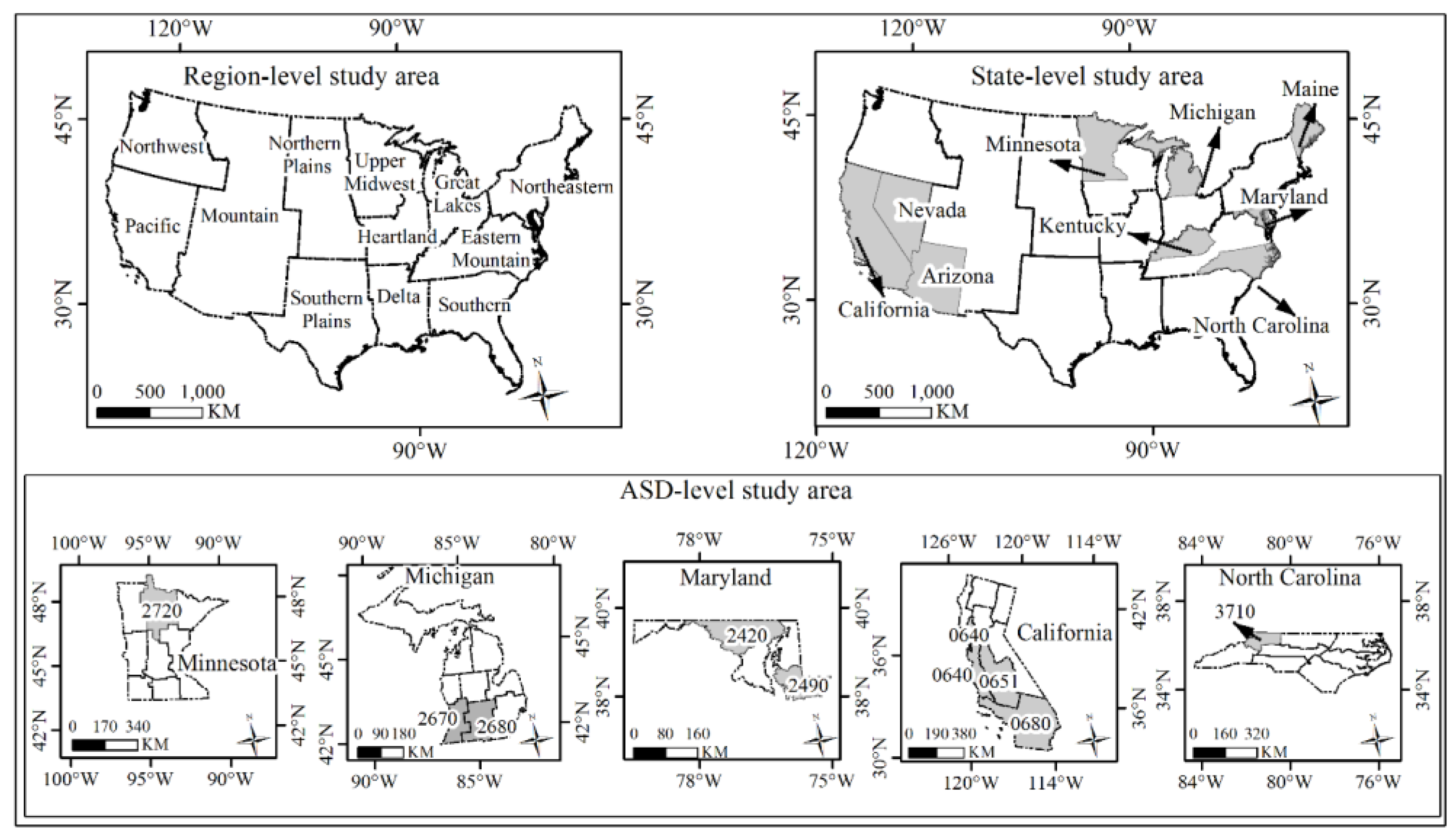
To analyze the influence of the size of the area on the upscaling accuracy, this research employed study sites for three different extents: regional level maps (a portion of the USA), US state level maps, and Agricultural Statistical District (ASD) level maps. The boundaries of the regions and the ASDs are defined by the USDA’s NASS. The U.S.A. has been divided into twelve regions (Figure 1). Each ASD is a group of counties based on the geography, climate, and cropping practice within each state [24], and has been widely-used in agricultural research (e.g., [11]).

To evaluate the landscape pattern of each of the study sites, the Patch-Per-Unit area (PPU) (Equation (1)), a measure of the heterogeneity [28], was employed to compute the heterogeneity for each study site. As the landscape becomes heterogeneous, PPU increases [28]. The crop/non-crop base maps derived from NASS’s CDL were utilized to compute the PPU for each state study site. The highest PPU for all states was 134.97, while the lowest was 4.72. The PPU (heterogeneity of each state) was then divided into three levels: lower level (0 < PPU ≤ 40), medium level (40 < PPU ≤ 100), and higher level (PPU >100). Three states were then selected for analysis from each of the three heterogeneity levels.

PPU = m/(n × λ),

(1)

where m is the total number of patches, n is the total number of pixels, λ is a scaling constant equal to the area of a pixel.

The PPU of each of the ASDs in the nine selected states were then calculated and divided into three different levels: lower level (0 < PPU ≤ 50), medium level (50 < PPU ≤ 120), and higher level (PPU >120). For each level of heterogeneity, three ASDs were randomly selected for analysis in this study. Therefore, we selected a total of twelve regions, nine states, and nine ASDs to be analyzed in this study. The landscape characteristics of these regions, states, and ASDs are shown in

Table 1. Landscape pattern for study sites at different levels. TA, NP and PLAND, respectively, represents the total area, the number of fields, and the proportion of crop in the landscape scenarios. Patch-Per-Unit area (PPU) measures the fragmentation of the study sites. Note that PPU were performed in kilometer square (km²) in this paper.

		TA (km2)	NP	PLAND	Mean Size of Fields (km2)	PPU
Regions	Heartland	326,626.3	178,538	36.44	1.83	54.66
	Mountain	1,734,205.4	238,082	6.93	7.28	13.73
	Northern Plains	796,517.3	479,110	38.72	1.66	60.15
	Northwest	642,992.8	82,452	8.46	7.80	12.82
	Pacific	696,249.9	64,637	5.50	10.77	9.28
	Upper Midwest	509,763.7	368,148	39.35	1.38	72.22
	Delta	382,528.1	109,111	17.81	3.50	28.52
	Eastern Mountain	508,588.4	334,785	13.68	1.51	65.83
	Great Lakes	351,437.4	249,684	33.18	1.40	71.05
	Northeastern	464,858.1	278,917	14.50	1.67	60.00
	Southern	513,624.9	202,950	9.35	2.53	39.51
	Southern Plains	866,793.2	219,485	13.35	3.95	25.32
States	Arizona	295,386.1	36,500	2.89	8.09	12.36
	California	409,884.8	89,759	8.59	4.57	21.90
	Kentucky	104,780.0	118,632	16.09	0.88	113.22
	Maine	84,430.3	34,942	3.93	2.41	41.39
	Maryland	26,193.8	34,777	29.46	0.75	132.77
	Michigan	150,745.8	139,808	23.31	1.07	92.74
	Minnesota	218,696.7	163,526	33.15	1.34	74.77
	Nevada	286,485.4	13,522	1.09	21.18	4.72
	North Carolina	128,187.2	140,766	15.78	0.91	109.81
ASDs	0640	41,552.6	10,371	3.82	4.01	24.96
	0651	71,221.8	41,474	27.60	1.72	58.23
	0680	118,264.7	10,448	2.59	11.32	8.83
	2420	9077.0	14,788	33.54	0.61	162.92
	2490	4582.1	3724	28.70	1.23	81.27
	2670	11,901.4	17,895	36.60	0.67	150.36
	2680	16,872.1	28,429	52.40	0.59	168.50
	2720	37,161.4	4261	1.52	8.72	11.47
	3710	8652.0	10,074	8.72	0.85	116.44

.

2.3. Description of the Similarity Matrix

The similarity matrix proposed here to evaluate the rescaling is based on a contingency table approach as shown in

Table 2. Similarity matrix to assess the accuracy of the upscaled maps.

		Upscaled Map
		Class 1	Class 2	Class i	Class k	Total
Base map	Class 1	A11	A12	A1i	A1k	A1+
	Class 2	A21	A22	A2i	A2k	A2+
	…	…	…	…	…	…
	Class i	…	…	Aii	…	Ai+
	…	…	…	…	…	…
	Class k	Ak1	Ak2	Aki	Akk	Ak+
	Total	A+1	A+2	A+i	A+k

. Each row represents the area of each class in the upscaled map, while each column represents the area of each class in the base map. A_ik denotes the area that is classified as class i in the base map but as class k in the upscaled map. Note that class k can be the same or different with class i. Entries on the diagonal represent the consistent area (i.e., similarity) for each class between the base map and the upscaled map. Thus, A_ii shows how many areas for class i are correctly identified in the upscaled map. A_+k sums the area of the class k in the upscaled map (the column total), and A_+i sums the area of the class i in the base map (the row total). The omission error (OE) for class i of the upscaled map can be evaluated by Equation (2), which represents the percentage of area for class i that is omitted from the upscaled map. The OE of class i also represents the underestimation of class i in the upscaled map. The commission error (CE) for class i can be evaluated by Equation (3), which represents the percentage of area for class i that is committed from the correct base map. The CE of class i represents the overestimation of the class i in the upscaled map. The overall similarity (OS) can be evaluated by Equation (4), which represents the percentage of the area for all classes that are correctly represented in the upscaled maps.

$$(A_{i+}-A_{ii})/A_{i+}$$

(2)

$$(A_{+i}-A_{ii})/A_{+i}$$

(3)

$${\displaystyle \sum _{i=0}^n{A}_{ii}}/{\displaystyle \sum _{i=0}^n{A}_{i+}=}{\displaystyle \sum _{i=0}^n{A}_{ii}}/{\displaystyle \sum _{i=0}^n{A}_{+i}}$$

(4)

2.4. Calculation of Similarity Matrix

To generate the similarity matrix, five steps should be taken:

• Compute the total number of the square windows ($N_{SW}$) to cover the base map. First, determine the total number of rows, M, and the total number of columns, N, for the upscaled map based on the desired spatial resolution (pixel size). Then, $N_{SW}$ is computed by $N_{SW}=M\times N$.
• Place $N_{SW}$ square windows (corresponding to the upscaled pixel size) over the base map. The square window, $W^{mn}$, corresponds to the pixel at row m and column n in the upscaled map.
• Identify the class type of the upscaled pixel corresponding to $W^{mn}$, which is denoted as class j (the entire upscaled pixel is class j). Then, identify the class types of the base map pixels within $W^{mn}$, which is denoted as class i.
• Calculate the area of class i of the base map pixels within $W^{mn}$. This area is denoted as $A_{ij}^{mn}$. Note that class i can be either the same or different than class j from the upscaled map. The area for class i in the base map that is classified as class j in the upscaled map, $A_{ij}$, can be computed by $A_{ij}={\displaystyle \sum _{\begin{array}{l}m=1,M\\ n=1,N\end{array}}{A}_{ij}^{mn}}$, which is used to fill in the values in the contingency table to obtain the similarity matrix.
• The OS, OE, and CE can be obtained to evaluate the accuracy of the upscaled map according to the principles in the Section 2.3.

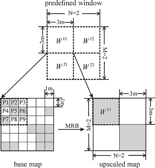
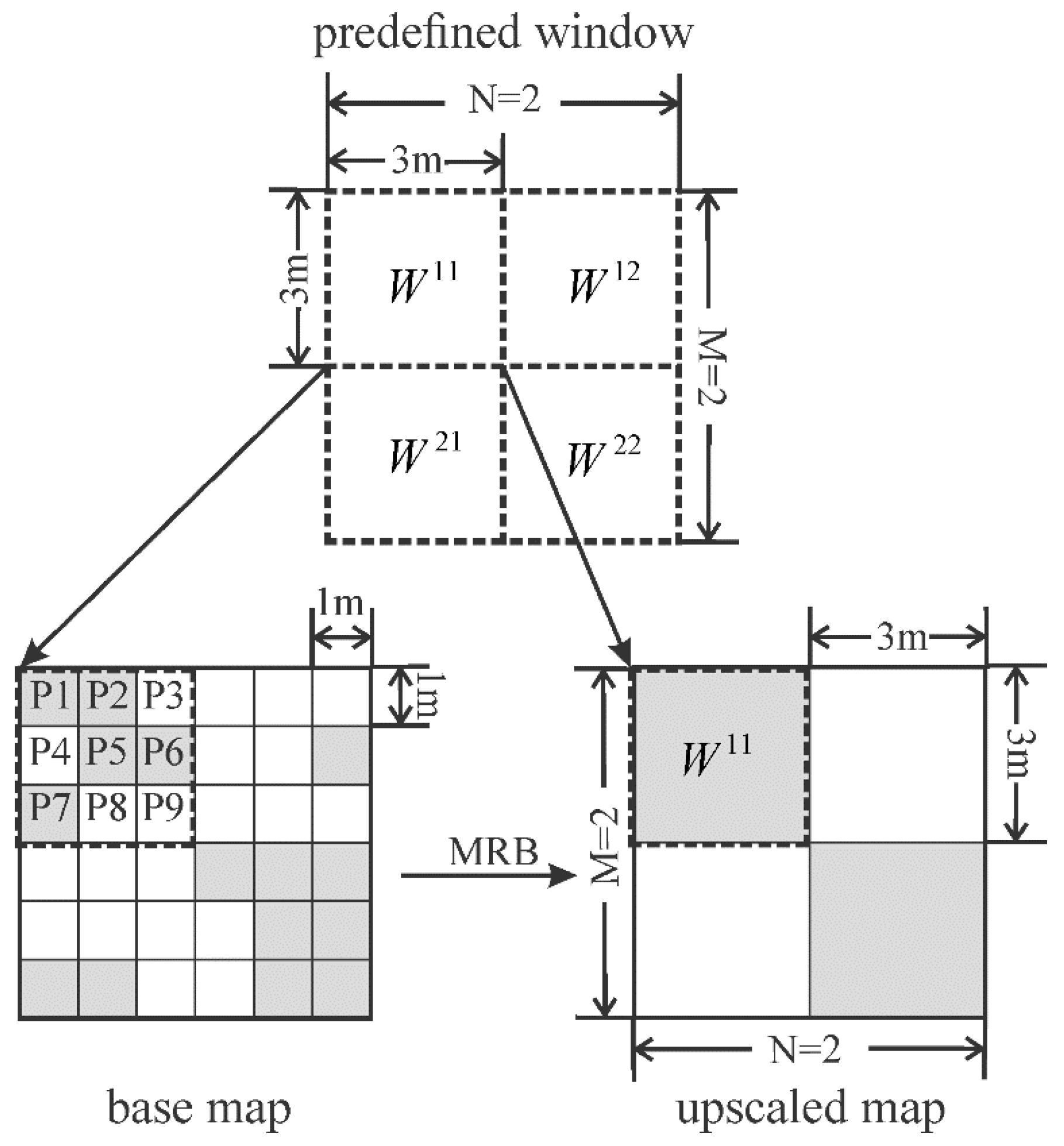
Figure 2 presents an example of generating the similarity matrix and will make this method much clearer. The base map covers an area of 36 m² and has a spatial resolution (pixel size) of 1 m (resulting in 36 pixels in this study area). There are two classes in this map; Class 1 (C1) is the gray color and Class 2 (C2) is the white color in both the base and upscaled maps. The desired spatial resolution of the upscaled map is 3 m.

Step 1: The number of square windows ($N_{SW}$) in the upscaled map is 4 (the number of rows is M = 2 and the number of columns is N = 2; 2 × 2 = 4).

Step 2: The computed windows are placed over the base map. The size of each square window is same as the spatial resolution (pixel size = 3 m) of the upscaled map.

Step 3: The class type of $W^{11}$ is C1 for the upscaled map as determined using the MRB upscaling method. The pixels within $W^{11}$ in the base map are marked as P1, P2, P3, P4, P5, P6, P7, P8, and P9 in Figure 2. The corresponding map classes are C1, C1, C2, C2, C1, C1, C1, C2, and C2, respectively.

Step 4: Compute $A_{ij}^{mn}$ for $W^{11}$. Then, $A_{11}^{11}=5$, $A_{21}^{11}=4$, $A_{12}^{11}=0$, and $A_{22}^{11}=0$. Thus, $A_{11}={\displaystyle \sum _{\begin{array}{l}m=1,2\\ n=1,2\end{array}}{A}_{11}^{mn}}=12$.

Repeat step 3 and step 4 to obtain $A_{ij}$ for $W^{12}$, $W^{21}$, $W^{22}$. For $W^{12}$, $A_{11}^{12}=0$, $A_{21}^{12}=0$, $A_{12}^{12}=1$, $A_{22}^{12}=8$. For $W^{21}$, $A_{11}^{12}=0$, $A_{21}^{12}=0$, $A_{12}^{21}=2$, $A_{22}^{21}=7$. For $W^{22}$, $A_{11}^{12}=7$, $A_{21}^{12}=2$, $A_{12}^{22}=0$, $A_{22}^{12}=0$. Then $A_{21}={\displaystyle \sum _{\begin{array}{l}m=1,2\\ n=1,2\end{array}}{A}_{21}^{mn}}=6$, $A_{12}={\displaystyle \sum _{\begin{array}{l}m=1,2\\ n=1,2\end{array}}{A}_{12}^{mn}}=3$, and $A_{22}={\displaystyle \sum _{\begin{array}{l}m=1,2\\ n=1,2\end{array}}{A}_{22}^{mn}}=15$.

Step 5:

Table 3. Similarity matrix for the example in Figure 2. OS, OE, and CE represent overall similarity, omission error, and commission error, respectively.

		Upscaled Map
		C1	C2	Total	OE (%)
Base map	C1	12	3	15	20.0
	C2	6	15	21	28.6
	Total	18	18
	CE (%)	33.3	16.7	OS = 75.0%

shows the results of similarity matrix for this example. Based on the similarity matrix, OE, CE and OS can be computed. The OS for this example is 75.0%. The CE and OE for this example can be found in Table 3.

2.5. Design of the Experiment

To investigate the performance of the similarity matrix on rescaling techniques, the upscaling method was selected to be used in this research. No analysis was performed for downscaling, but the approach should work the same. The crop/non-crop maps were upscaled based on a widely-used aggregation method (i.e., MRB). The details of the MRB are described in Section 2.6. The similarity matrix was then obtained to illustrate the accuracy of the upscaled maps.

To explore if existing, coarser resolution land cover maps are better than newly created upscaled maps derived from accurate and finer resolution land cover maps, existing land cover maps at two different resolutions (240 m and 960 m) were chosen. Note that we are aware that producing land cover maps at coarse resolutions are vitally important for various research projects. Thus, our work here only aims to develop a tool (i.e., the similarity matrix) for evaluating the upscaled maps. It is not our intent to minimize the contributions of the existing, coarser resolution land cover maps for the Earth science community.

2.6. Upscaling Method

The MRB method for upscaling categorical maps has been recommended by [15] for agricultural projects. Therefore, our work utilized this method as an appropriate way to obtain the upscaled maps. To implement the MRB, a predefined square window corresponding to the coarser resolution pixel is constructed. Then, the MRB assigns the class type for the coarser resolution pixel based on selection of the most frequently occurring class in the base map within the predefined square window [17,18]. If there is more than one major class in the square window, the class for the coarser resolution map will be randomly determined from these major classes [15]. In this work, the base map was upscaled to 240 m and 960 m, respectively.

3. Results

The CDL data were used to generate the crop/non-crop base maps which were then used to create the upscaled maps at 240 m and 960 m spatial resolution for each study site. The similarity matrix, proposed here was then employed to assess the accuracy of these upscaled maps. This assessment method can not only quantify how well the upscaling techniques represent the area of all the land cover types, but also the omitted and committed area information for each map class. The accuracy of the GFSAD maps was estimated using a similarity matrix for comparison with the upscaled maps. After assessing the upscaled maps and the GFSAD maps, there were four issues of concern left to be analyzed: (1) a comparison of the accuracy of the upscaled maps and the GFSAD maps; (2) a comparison of the study site heterogeneity between the upscaled maps and the GFSAD maps; (3) the influence of heterogeneity on the accuracy of upscaled maps and GFSAD maps, and (4) the influence of extent on the accuracy of the upscaled maps.

3.1. Accuracy Assessment and Comparisons of Upscaled and GFSAD Maps

There are a total of 30 base maps generated from CDL data for all study sites (12 regions + 9 states + 9 ASDs). For each study site, two upscaled maps (at 240 m and 960 m) were generated using these base maps. Figure 3 shows an example of these base map and the corresponding upscaled maps for the Heartland region study area. The results show that the upscaled maps have different spatial distributions of the land cover from the base map. In addition, the upscaled maps visually show that the difference in the spatial distribution of the land cover became larger as the upscaled map became coarser.

The similarity matrix for each upscaled map and each GFSAD map was obtained using the procedure developed in this project. An example of the similarity matrix for the upscaled map at 240 m for the Heartland region study site is shown in

Table 4. An example of similarity matrix for the upscaled map at 240 m of the Heartland region. The unit of area is km².

		Upscaled Map
		Non-Crop	Crop	Total	OE (%)
Base map	Non-crop	192,370.09	15,044.26	207,414.346	7.82
	Crop	11,638.43	107,291.75	118,930.176	9.79
	Total	204,008.52	122,336.01
	CE (%)	5.70	12.30	OS = 91.82%

. The results show that the crop was omitted 9.79% and committed 12.30% of the time in the 240 m upscaled map. The OS for this example is 91.82%.

Table 5. The Overall Similarity (OS) of the upscaled maps for all study sites.

Regional Level			States Level			ASD Level
Study Site	240 m	960 m	Study Site	240 m	960 m	Study Site	240 m	960 m
	OS (%)			OS (%)			OS (%)
Heartland	91.82	86.88	Arizona	98.98	98.63	0640	97.87	97.12
Mountain	97.78	96.44	California	98.05	97.28	0651	94.67	92.55
Northern Plains	89.53	82.53	Kentucky	91.29	88.42	0680	99.26	98.96
Northwest	97.89	96.49	Maine	97.34	96.40	2420	83.87	76.39
Pacific	98.67	98.12	Maryland	87.03	79.97	2490	89.55	80.41
Upper Midwest	90.00	84.94	Michigan	91.47	87.06	2670	85.49	77.67
Delta	95.60	93.35	Minnesota	92.57	88.47	2680	83.32	73.85
Eastern Mountain	91.99	89.15	Nevada	99.57	99.32	2720	99.09	98.73
Great Lakes	90.21	84.87	North Carolina	91.01	86.91	3710	92.70	91.47
Northeastern	92.16	88.70
Southern	94.62	92.55
Southern Plains	96.09	93.32

presents a summary of the OS for all of the upscaled maps (12 regions, 9 states, and 9 ASDs).

Table 6. The Omission Error (OE) and Commission Error (CE) for the crop map class in the upscaled maps for all study sites.

Resolution	Region	OE (%)	CE (%)	State	OE (%)	CE (%)	ASD	OE (%)	CE (%)
240 m	Heartland	9.79	12.30	Arizona	21.99	14.58	0640	36.54	23.11
960 m		17.37	18.40		30.26	19.77		54.25	31.50
240 m	Mountain	18.92	13.86	California	10.65	11.92	0651	7.17	11.56
960 m		32.36	21.97		14.64	16.56		9.17	16.36
240 m	Northern Plains	12.21	14.45	Kentucky	37.95	20.68	0680	16.67	12.45
960 m		21.21	23.28		53.78	28.15		24.19	17.47
240 m	Northwest	12.40	12.56	Maine	50.40	25.84	2420	26.68	22.51
960 m		21.30	20.34		82.37	34.79		39.41	33.54
240 m	Pacific	11.94	12.16	Maryland	25.48	19.78	2490	20.05	16.76
960 m		17.16	16.95		41.06	31.05		40.60	30.90
240 m	Upper Midwest	11.42	13.63	Michigan	18.81	17.96	2670	20.48	19.41
960 m		17.82	19.92		29.98	26.62		33.31	29.31
240 m	Delta	13.19	11.73	Minnesota	9.81	12.25	2680	14.20	17.04
960 m		19.43	18.13		15.38	18.67		20.27	27.09
240 m	Eastern Mountain	41.36	22.69	Nevada	26.56	15.18	2720	44.19	22.03
960 m		63.10	30.44		45.31	23.68		69.87	32.41
240 m	Great Lakes	13.94	15.31	North Carolina	38.71	22.89	3710	68.42	32.68
960 m		21.83	23.26		65.80	33.12		92.42	42.61
240 m	Northeastern	33.63	23.55
960 m		56.62	32.85
240 m	Southern	40.21	22.41
960 m		62.97	30.96
240 m	Southern Plains	16.92	12.99
960 m		30.00	22.28

presents a summary of the OE and CE for the crop map class in all of the upscaled maps. At all spatial extents and study sites, the OS decreased and OE and CE increased when the upscaled maps became coarser. For example, the OS for the Heartland study site decreased from 91.82% to 86.88% and OE and CE increased from 9.79% to 17.37%, and from 12.3% to 18.40% when the basemap was upscaled from 240 m to 960 m.

Table 7. The Overall Similarity (OS) of the Global Food Security-Support Analysis Data (GFSAD) maps for each study site.

Regional Level			State Level			ASD Level
Study Site	240 m	960 m	Study Site	240 m	960 m	Study Site	240 m	960 m
	OS (%)			OS (%)			OS (%)
Heartland	85.43	41.93	Arizona	98.38	84.80	0640	96.49	44.51
Mountain	95.83	57.20	California	94.35	72.20	0651	81.04	50.16
Northern Plains	80.60	39.92	Kentucky	87.51	35.57	0680	98.22	82.89
Northwest	96.03	57.20	Maine	96.22	59.34	2420	71.08	42.53
Pacific	96.32	77.06	Maryland	77.69	38.80	2490	80.96	45.48
Upper Midwest	83.89	53.08	Michigan	84.86	52.85	2670	75.30	38.59
Delta	91.77	48.92	Minnesota	87.88	54.75	2680	69.74	52.42
Eastern Mountain	88.67	31.81	Nevada	99.13	83.96	2720	98.63	47.08
Great Lakes	81.63	46.83	North Carolina	86.37	27.93	3710	91.37	29.12
Northeastern	87.39	40.15
Southern	91.66	43.27
Southern Plains	92.50	41.25

presents the OS for all GFSAD maps for all of the study sites and

Table 8. The Omission Error (OE) and Commission Error (CE) for the crop map class in the GFSAD maps.

Resolution	Study Site	OE (%)	CE (%)	Study Site	OE (%)	CE (%)	Study Site	OE (%)	CE (%)
240 m	Heartland	28.09	14.19	Arizona	43.34	18.45	0640	84.26	31.94
960 m		0.06	61.44		15.09	85.74		14.42	94.38
240 m	Mountain	48.70	18.27	California	57.12	16.71	0651	60.25	17.44
960 m		5.61	86.64		2.41	76.66		0.49	64.41
240 m	Northern Plains	32.53	20.65	Kentucky	70.60	19.12	0680	52.59	25.34
960 m		0.03	60.81		0.58	80.08		9.92	87.86
240 m	Northwest	31.28	18.51	Maine	94.76	21.87	2420	78.06	27.08
960 m		1.75	83.66		25.14	93.09		1.80	63.32
240 m	Pacific	58.68	16.60	Maryland	65.75	20.99	2490	55.29	19.60
960 m		5.19	81.26		4.76	67.71		8.09	66.39
240 m	Upper Midwest	27.39	15.73	Michigan	51.23	21.89	2670	50.74	25.36
960 m		0.31	54.36		2.96	67.13		0.79	62.73
240 m	Delta	37.56	12.14	Minnesota	22.38	15.45	2680	38.78	23.65
960 m		1.71	74.17		0.15	57.73		0.56	47.58
240 m	Eastern Mountain	75.05	23.58	Nevada	76.41	14.44	2720	80.56	32.63
960 m		2.40	83.54		36.62	95.78		8.86	97.44
240 m	Great Lakes	41.43	19.19	North Carolina	74.41	31.63	3710	97.74	36.34
960 m		0.99	61.59		2.41	82.24		3.29	89.35
240 m	Northeastern	81.07	23.40
960 m		4.85	81.02
240 m	Southern	82.96	26.56
960 m		14.38	87.30
240 m	Southern Plains	43.18	18.66
960 m		3.11	81.84

shows the OE and CE for the crop map class in all of the GFSAD maps. The OS of GFSAD maps at 960 m were, for many of the sites, significantly lower than the OS of the GFSAD maps at 240 m. For example, the OS for the Mountain region at 960 m decreased by 38.63 percentage points compared to the OS at 240 m. Additionally, the OE of the GFSAD maps at 960 m were lower than at 240 m, while CE at 960 m were higher when compared to the 240 m map.

To achieve one of the primary objectives of this paper, the accuracies of the upscaled maps and the GFSAD maps were compared. Table 5, Table 6, Table 7 and Table 8 show that the upscaled maps obtained higher accuracy (higher OS, lower OE and CE) when compared to the GFSAD maps at each of the three different extent levels. For example, the OS of the upscaled map at 240 m for the Heartland region study site was higher by 6.39 percentage points compared to the coarse resolution GFSAD map at 240 m (Table 5 and Table 7). Also, the OE and CE for the crop class of the upscaled map at 240 m for the Heartland region study site were lower by 18.3 percentage points and 1.89 percentage points, respectively, compared to the GFSAD map at 240 m.

3.2. Comparisons of Heterogeneity between Upscaled Maps and GFSAD Maps

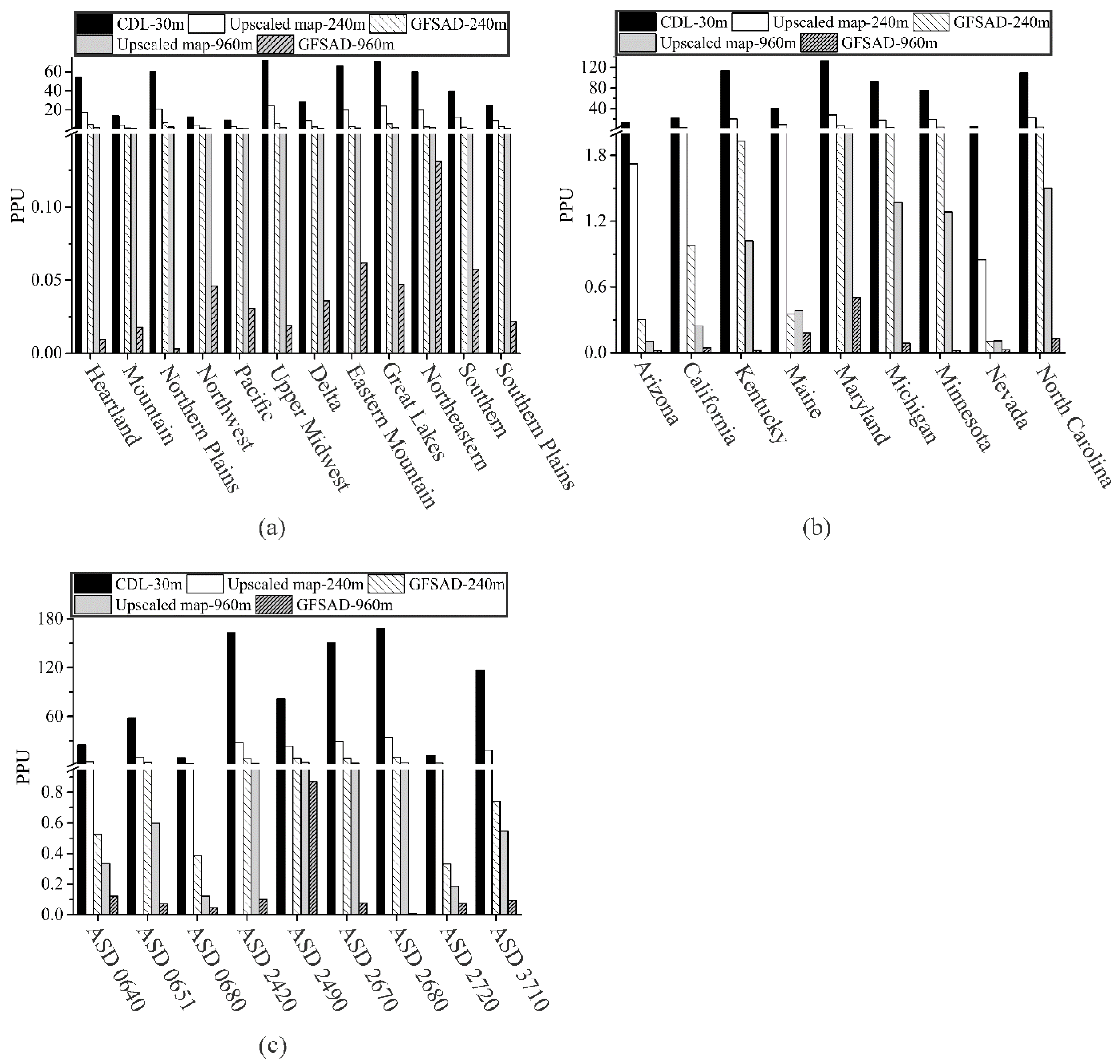
Figure 4 presents the PPU of the crop/non-crop map at 30 m (the reference data), the upscaled maps and the GFSAD maps for comparison. The results show that the PPU of the upscaled maps are closer to the PPU of the reference data compared to the PPU of the GFSAD maps. For example, for the Northern Plains region study site, the PPU of the reference data, the upscaled map at 240 m, and the GFSAD map at 240 m, were 60.15, 21.05, and 6.85, respectively. Additionally, the PPU of the maps at 240 m (either upscaled maps or GFSAD maps) are closer to the PPU of the reference data compared to the PPU of the coarser resolution maps at 960 m. For example, for the Heartland region study site, the PPU of reference map, the upscaled maps at 240 m and 960 m were 54.66, 17.53, and 1.31, respectively.

3.3. Influence of Heterogeneity on Upscaled Maps and GFSAD Maps

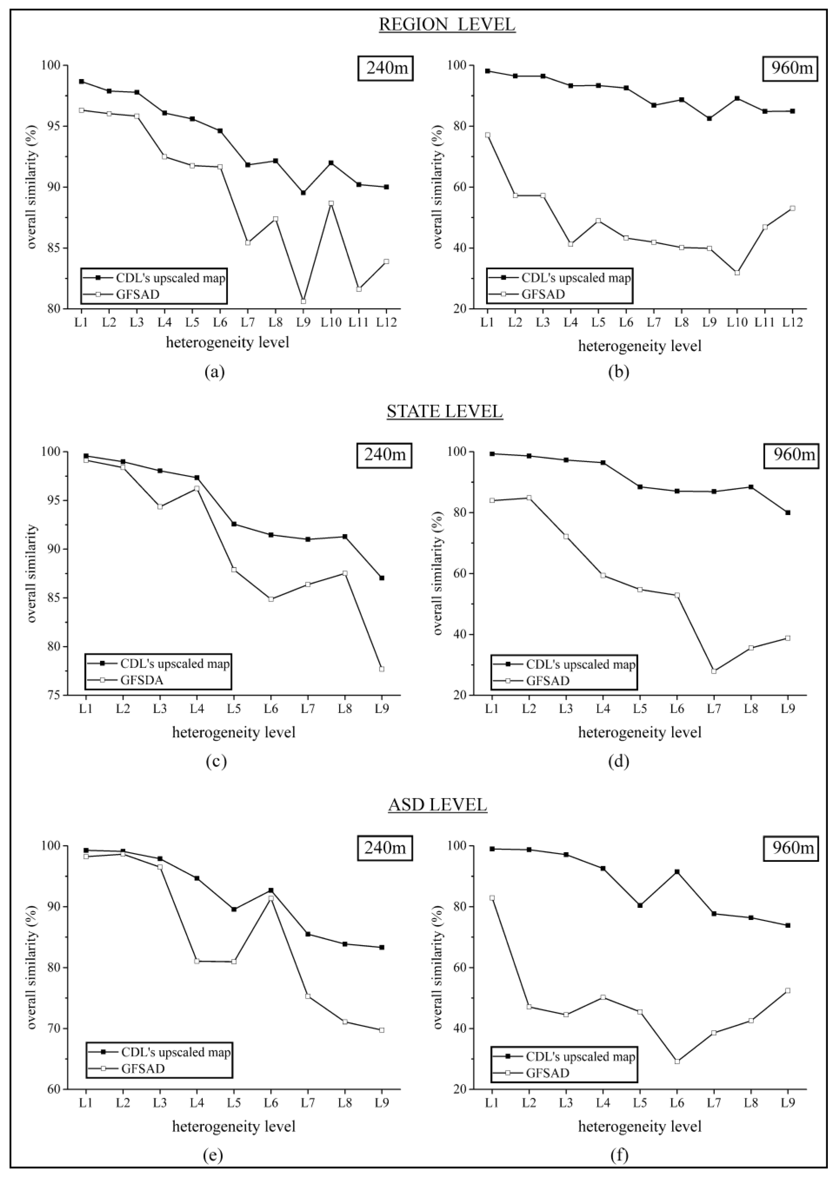
Figure 5 shows the relationship between the OS of either the upscaled maps or the GFSAD maps and the heterogeneity of each grouping of study sites by extent (i.e., regional, state, and ASDs). The study sites at each spatial extent were grouped into one of several heterogeneity levels (L1 to Lh) based on their PPU. For example, there are a total of 12 region level study sites, thus, the heterogeneity was defined as 12 levels (Figure 5a,b), which increased corresponding to L1, L2, …, L12. The results show that higher heterogeneity results in lower accuracy of the upscaled maps and the GFSAD maps at each resolution. For example, when the PPU increased from 9.28 to 72.22 (heterogeneity level L1 to L12 in Figure 5), the OSs for the region-level study sites were reduced from 98.67% to 90.00%, and from 96.32% to 83.89%, respectively, for the upscaled map at 240 m and the GFSAD map at 240 m (Figure 5a). Additionally, either OE, CE, or both increased for the upscaled and the GFSAD maps when the study site became more heterogeneous (Table 6 and Table 8). For example, Maryland with PPU of 132.77 was more heterogeneous than the Nevada with PPU of 4.72. For the Maryland, the CE for crop of the GFSAD map at 240 m was higher by 6.55 percentage points, comparing to the Nevada (Table 8).

3.4. Influence of Extent on the Accuracy of Upscaled Maps

The results show that the extent of the study sites did not impact the accuracy of upscaled maps. First, for some study sites, there is no influence on the accuracy of the upscaled maps when the extent of the study site changes. For example, the state of Arizona and the ASD2720 had similar landscape pattern (landscape heterogeneity, and mean size of the fields (Table 1)). Note that the Arizona covered about 295,386.1 km² that is about eight times larger than ASD2720 which is located in Minnesota (Table 1). The OS of upscaled maps at 960 m for these two study sites were 98.63%, and 98.73%, respectively (Table 5).

Second, for some other study sites, the accuracy of the upscaled maps for the regions (i.e., the very large areas) varied such that some were lower and others higher than the small areas. For example, the Northwest region covered about 642,992.8 km² which is about 17 times larger than the ASD2720 (Table 1). The OS of upscaled map at 240 m for the Northwest region was lower by about 1.2 percentage points compared to the ASD2720 (Table 5).

4. Discussion

4.1. Significance of the Similarity Matrix

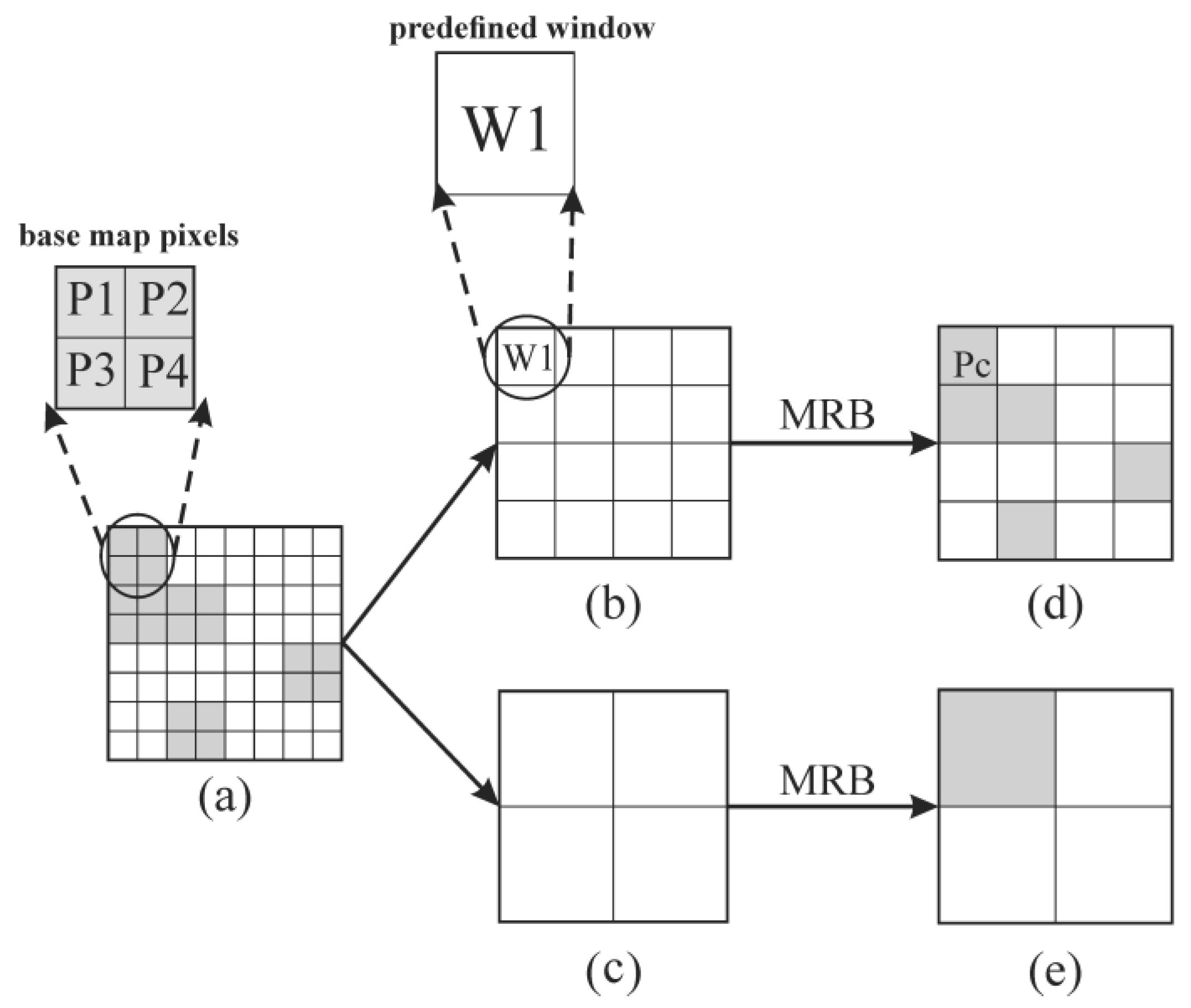
Rescaling techniques inevitably lead to errors in land cover area (e.g., [11,14]). These errors in area are not only derived from the omitted areas from the base map but also by the committed areas created in the upscaled map. If the OS is 100% (i.e., the base map and the upscaled map are exactly the same (Figure 6a,d), it is not necessary to compute the OE and CE. However, an OS of 100% rarely occurs (e.g., [11]). Even if the OS of 100% occurs at a particular spatial resolution, it is difficult to know if the OS will also be 100% at another spatial resolution. Figure 6 shows an example where the base map (Figure 6a) is upscaled by the MRB to two different spatial resolutions (Figure 6d,e). Figure 6b,c are predefined windows for producing Figure 6d,e, respectively. The gray color represents class 1, while the white color represents class 2. In some situations, the area information of one class in the upscaled map will be same as its area information in the base map. For example, the base map pixels, P1, P2, P3, and P4, were aggregated to upscaled pixel Pc (Figure 6d). Since class 2 occurred more frequently within the predefined window, W1, the class type of Pc is class 2 according to the principle of MRB. However, the OS cannot be always 100% due to the CE and OE. For example, In Figure 6d, the OS is 100%, while in Figure 6e the OS is 81.25%. Up to now, there has been no standard and simple way to evaluate the accuracy of the rescaled map and to report the uncertainty information of the rescaled map to the users of the land cover map. The similarity matrix proposed here provides such a way.

4.2. Issues for Generating Upscaled Maps

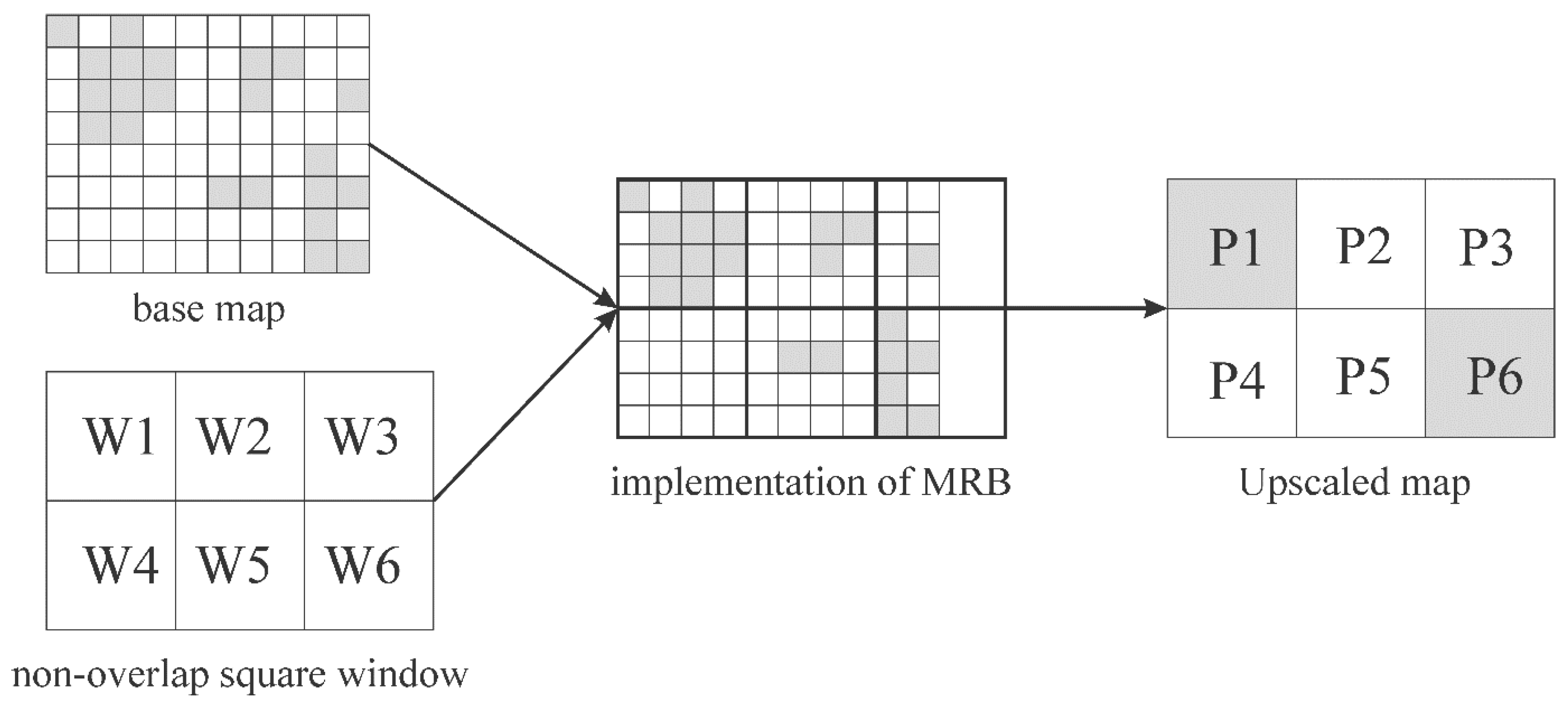
An important upscaling issue that should be noted here is the problem that can occur around the edges of the study area. If the dimensions of the base map and the rescaled map are not equally divisible, then some partial upscaled pixels will fall outside of the edge of the base map. As Figure 7 demonstrates, two non-overlapping windows (W3 and W6) fall outside the edge of the base map. The upscaled pixels, P3 and P6, are determined based on only the pixels in the base map that fall within the W3 and W6. Thus, for W3 and W6, there are only eight pixels used to determine the class type in the upscaled map.

Interactive Data Language (IDL 8.3) was used to conduct MRB rescaling in this project. For this language, the implementation of the MRB rescaling algorithm begins from the upper-left pixel as the first pixel and ends with the lower-right pixel as the last pixel. Hence, the potential error of the determination of the boundary pixel in an upscaled map only occurs at the right edge and/or the bottom edge of the upscaled map. However, the similarity matrix is not impacted because only existing class types are included in the matrix calculation. In addition, the similarity matrix presents the uncertainty information by considering the error derived from the boundary pixels in the upscaled maps. These conditions further strengthen our confidence to recommend the similarity matrix to be extensively used to evaluate the rescaled maps.

4.3. Accuracy Analysis between Upscaled Maps and GFSAD Maps

Since one of our objectives was to compare existing coarser resolution maps with the upscaled maps, the GFSAD maps also were assessed using the similarity matrix. One issue that should be noted is that the crop/non-crop maps derived from the CDL data were assumed as the reference data for assessing the GFSAD maps [29]. We are aware that the CDL data are not 100% accurate. However, this dataset is highly accurate and was readily available at finer resolution [7] and therefore, was very appropriate for use in this project.

The comparisons of accuracy between the upscaled maps and GFSAD maps show that the upscaled maps can obtain higher accuracies (Table 5, Table 6, Table 7 and Table 8). These results demonstrate that employing upscaled maps will be a better way to further conduct the related earth modeling research compared to using the GFSAD maps. Note that we are not saying here that all the existing coarser resolution maps should be replaced by the upscaled maps, but rather that the similarity matrix should be used to test which is better.

The lower accuracy of the GFSAD map in the USA mainly results from fact that coarser spatial resolution imagery were used for producing the GFSAD maps, while the finer spatial resolution imagery were used for producing the CDL data. The finer resolution imagery used to generate the CDL data include Lansat-5 Thematic Mapper (TM), Landsat-7 Enhanced TM plus (ETM+), Landsat-8 Optical Land Imager (OLI), Resourcesat-1 Advanced Wide Field Sensor (AWiFS), Disaster Monitoring Constellation (DMC) DEIMOS-1, and UK2 sensors. This finer-resolution imagery was used to obtain base maps that can accurately represent the distribution of land cover. However, the GFSAD maps are mainly based on the MODerate resolution Imaging Spectroradiometer (MODIS) imagery at 250 m [29]. As is known, greater amounts of mixed pixels exist in the coarser resolution imagery, which can introduce more errors into the classified maps (i.e., GFSAD map) [30]. Therefore, compared to the upscaled maps derived from accurate, finer resolution CDL data, GFSAD likely will not obtain higher accuracy of the distribution of land cover.

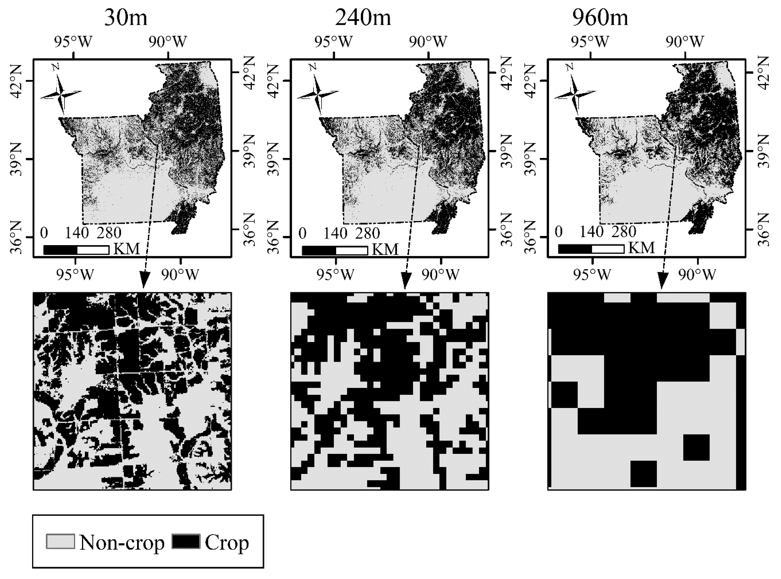
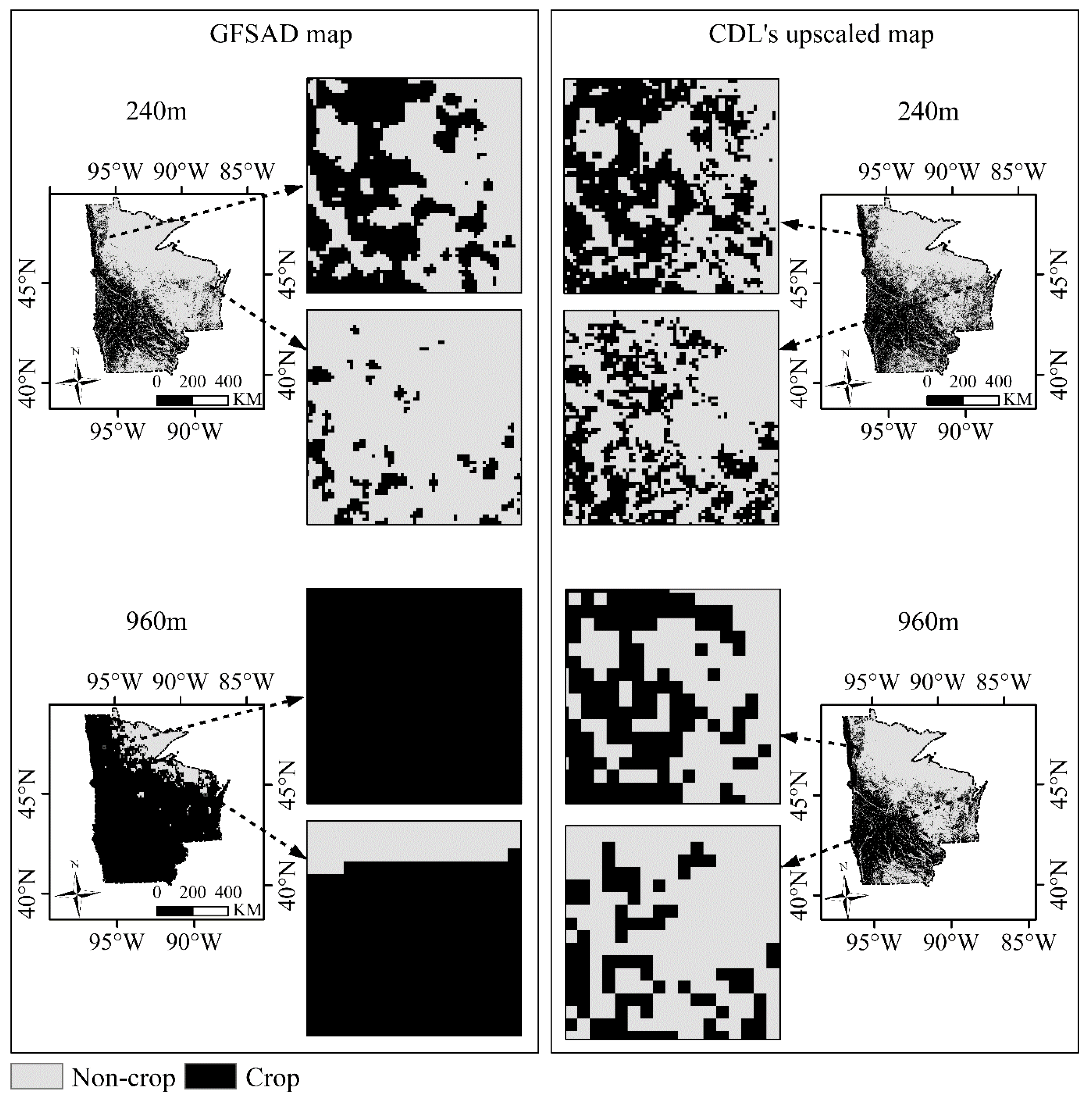
To visually show the difference between the upscaled map and the GFSAD map, two sub-areas in the region of Upper-Midwest were selected (Figure 8). The upscaled map either at 240 m or at 960 m accurately presents the crop distribution. The GFSAD map at 960 m of the region was mostly classified as crop, while the upscaled map present the original crop distribution as accurate as possible. These results demonstrate that the upscaled map can more accurately represent the distribution of land cover, which further strengthens our confidence in recommending the use of upscaled maps as inputs for earth science models. However, assessing and comparing the performance of the upscaled maps and existing coarser resolution maps are required before making these decisions.

4.4. Differences in Heterogeneity between the Upscaled Maps and the GFSAD Maps

A vitally important issue underlying different land cover maps is the difference in representations of landscape pattern. As acknowledged, several studies have reported that the representation of landscape pattern is biased in the upscaled map (e.g., [11,15]). However, comparisons between the representation of landscape pattern based on the upscaled map and the existing coarser resolution map has not been explored. Therefore, the heterogeneity, evaluated by PPU, was selected to be analyzed in this research. Note that the study sites with higher PPU are more heterogeneous than study sites with lower PPU.

The comparisons of heterogeneity represented by the PPU values (Figure 4) and by visual observation (Figure 8) between the upscaled maps and the GFSAD maps demonstrated that upscaled maps can obtain a better representation of the landscape patterns when compared to the GFSAD maps. This is because the upscaled maps can more accurately represent the distribution of land cover compared to the GFSAD maps. Furthermore, for users, a good quality land cover map should not only have a better map accuracy, but also a better representation of landscape pattern. Therefore, considering the comparisons of the PPU between two datasets and the users’ requirements, the upscaled map is more suitable and should be used in Earth science models.

4.5. Considerations with Respect to Heterogeneity

The heterogeneity of the study site has been emphasized as a major factor impacting the accuracy of the upscaled maps (e.g., [11,31]) and the accuracy of classification maps (e.g., [32]), in general. Thus, the influence of heterogeneity on upscaled maps and GFSAD maps should be explored. As expected, the accuracies of both the upscaled maps and the GFSAD maps were considerably impacted by the heterogeneity of the study sites. Lower accuracies for the upscaled and the GFSAD maps, at each resolution, were obtained in the more heterogeneous areas compared to the homogeneous areas (Figure 5, Table 5, Table 6, Table 7 and Table 8). This is because the spectral heterogeneity and spectral complexity of the imagery are higher in heterogeneous areas, which results in lower classification map accuracy (e.g., CDL data, GFSAD map) [32]. If these heterogeneous maps (e.g., CDL data) were used as base maps for upscaling, mapping error would increase in the upscaled map and the accuracy of the upscaled map would be reduced [11]. Therefore, given the lower upscaling accuracy in the heterogeneous areas, users should be cautious when utilizing upscaled maps in heterogeneous landscapes.

Recognizing the negative effect of heterogeneity on the upscaled maps requires not only that caution be taken when using the upscaling techniques in the heterogenous areas, but also demonstrates the need for developing improved upscaling techniques. The improved upscaling techniques should consider the heterogeneity as a factor to improve the upscaling accuracy. Additionally, the analyst that is producing the land cover map should be aware of lower accuracy occurring in the heterogeneous areas. More accurate and improved classification techniques are also recommended to be developed and employed for improving the accuracy of the land cover products, especially in the heterogeneous areas. These accurate land cover products can be further used for producing upscaled maps at different resolution meeting the requirements for various Earth observation models or their related research (e.g., [33]).

4.6. Considerations with Respect to Extent of Maps

Landscape pattern has strong influence on the accuracy of the upscaled maps, as demonstrated by previous research (e.g., [31,34]). However, previous research rarely explored if the extent (i.e., size of the area) of the study sites impacted the upscaled maps. Therefore, as part of our research we employed different size study sites from large regions of the US to individual states, to smaller ASDs within a state. Although we did not test different upscaling methods to see if extent has an influence on the upscaling accuracy, it is worthy of discussion based on the results derived from using just the MRB approach.

The results of this study demonstrated that there was no difference between upscaled maps at the same spatial resolution for different extent levels (i.e., region level, state level, and ASD level). As long as the heterogeneity is similar, the upscaling accuracy did not show much difference between study area sizes. Instead, it is evident that heterogeneity and not extent is the main factor impacting the upscaling accuracy.

4.7. Implications, Limitations, and Future Work

The results of this work have important implications for decision making. The similarity matrix has been demonstrated as an efficient and effective method to assess the rescaled map. This method can provide detailed information on the accuracy of the rescaled map, which is important for users who wish to use these maps for further applications. In addition, comparisons between the upscaled map and any existing coarser resolution map draw demonstrate that it may be better to use the upscaled map than an existing coarser resolution map. The higher performance of the upscaled maps, in terms of accuracy and landscape pattern, confirms that they can be reliably used for Earth science modelling. Note that, here, we did do not emphasize the upscaled maps can always be better than the existing maps. The results illustrate that the upscaled maps can be one option for map users. Therefore, we strongly recommend that a comparison using the similarity matrix should be conducted to assess any existing coarse resolution maps with potential upscaled maps for use in any modelling.

Further, the role of heterogeneity in producing upscaled maps confirms that landscape pattern is an important consideration for those researchers developing upscaling techniques to obtain more accurate upscaled maps. Moreover, this study provides evidence that it is not necessary to consider the extent when developing a new upscaling technique. Overall, the achievements of this paper are essential for guiding land cover map users to select suitable datasets for their models and encourage them to consider heterogeneity when developing any new upscaling techniques.

Finally, we are aware that our research may have three limitations. The first major limitation is that there was no GFSAD map at 30 m resolution for 2010. Therefore, we used the CDL data at 30 m to generate the crop/non-crop map as the reference data to compare the results between GFSAD maps and the upscaled maps. These comparisons were based on the assumption that the CDL data are 100% correct, which we acknowledge is not the case. This limitation resulted in errors in the final results, which would be extremely difficult to quantitatively assess without an extremely accurate reference data. In order to do this assessment, reference data covering the entire USA would be needed. The cost for producing such a dataset in prohibitive and justifies our use of a very accurate (not 100%) data set (e.g., CDL).

The second limitation is that the results of this paper are based on the simple case of a crop/non-crop map and not a more complex land cover map with many land cover classes. Thus, our analysis should be repeated in future work using upscaled maps and the existing land cover maps that are more complex. Additionally, only the upscaling of maps has been explored in this paper. While these techniques are directly applicable to downscaled maps, the paper does not demonstrate this use and should be the subject of future work.

The third limitation is that only a single upscaling technique (i.e., MRB) was used here. As acknowledged, different upscaling techniques perform differently (e.g., [15]). The goal of this paper was to demonstrate the power of the similarity matrix and not to evaluate upscaling algorithms. Therefore, it would be useful to use the similarity matrix approach to compare different upscaling techniques in some future work.

5. Conclusions

This paper first proposed a new method, the similarity matrix, for assessing the accuracy of rescaled maps using three measurements: overall similarity (OS), omission error (OE), and commission error (CE). A conventional upscaling technique, Majority Rule Based aggregation (MRB), was used to produce the upscaled maps to demonstrate the performance of the similarity matrix. Additionally, this paper explored if these upscaled maps perform better than existing coarse resolution crop/non-crop maps. To conduct these experiments, two datasets: the Cropland Data Layer (CDL) at 30 m for 2010 and the GFSAD nominal data for 2010 at 250 m and 1 km, were utilized. The CDL data were first used to extract the crop/non-crop maps for (1) providing the base maps for upscaling, and (2) providing reference data to assess the accuracy of the upscaled maps and the GFSAD maps. Further, to determine if the extent of the study site has influence on the performance of the upscaling, three different extent levels were employed. There were twelve regions covering the continental USA, nine states, and nine Agricultural Statistic Districts (ASDs) that were selected to perform the experiments. Several conclusions resulted from this analysis: (1) the similarity matrix can successfully assess the accuracy of the rescaled map and report the uncertainty information for the rescaled map. This information is beneficial for land cover map users for further assessing the uncertainty or accuracy of their models. Also, the similarity matrix can provide information for making decisions about selecting the datasets for further analysis such as use in Earth science modeling; (2) the upscaled maps outperformed the existing coarser resolution GFSAD maps in both accuracy and representation of the landscape pattern. This result demonstrates that evaluating the performance of the upscaled map and the existing coarser resolution map is required before making a decision for selecting the datasets as the input to the users’ model; (3) the influence of heterogeneity on the upscaling accuracy does not only reveal that lower accuracy was produced in the heterogeneous area, but also recommends that a new upscaling technique should consider heterogeneity as an important factor to improve the accuracy of the upscaling technique, and (4) the results between different study sites with different extents quantitatively confirms that the performance of upscaling has not been impacted by the extent of study site. In conclusion, extending our understanding on how to assess the rescaled map, determination for selecting the upscaled map or the existing land cover map, and suggestions for developing new upscaling techniques, is vitally helpful to the Earth science community as users of land cover maps.

Future work should focus on four aspects: (1) different downscaling/upscaling techniques should be employed to investigate if the downscaled/upscaled maps can really perform better than the existing land cover maps; (2) comparisons between upscaled maps and downscaled maps should be demonstrated; (3) landscape pattern should be considered for developing new downscaling/upscaling techniques, and (4) the land cover map with more map classes should be employed to explore if the upscaled map and downscaled map still can be a prospective data source for Earth science modelling research.

References

- Congalton, R.G.; Gu, J.; Yadav, K.; Thenkabail, P.; Ozdogan, M. Global land cover mapping: A review and uncertainty analysis. Remote Sens. 2014, 6, 12070–12093. [Google Scholar] [CrossRef]
- Wang, Z.; Hoffmann, T.; Six, J.; Kaplan, J.O.; Govers, G.; Doetterl, S.; Oost, K.V. Human-induced erosion has offset one-third of carbon emissions from land cover change. Nat. Clim. Change 2017, 7, 345. [Google Scholar] [CrossRef]
- Pachauri, R.K.; Allen, M.R.; Barros, V.R.; Broome, J.; Cramer, W.; Christ, R.; Church, J.A.; Clarke, L.; Dahe, Q.; Dasgupta, P.; et al. Climate Change 2014: Synthesis Report. Contribution of Working Groups I, II and III to the Fifth Assessment Report of the Intergovernmental Panel on Climate Change; Pachauri, R.K., Meyer, L., Eds.; IPCC: Geneva, Switzerland, 2014. [Google Scholar]
- Sellers, P.J.; Dickinson, R.E.; Randall, D.A.; Betts, A.K.; Hall, F.G.; Berry, J.A.; Collatz, G.J.; Denning, A.S.; Mooney, H.A.; Nobre, C.A.; et al. Modeling the exchanges of energy, water, and carbon between continents and the atmosphere. Science 1997, 275, 502–509. [Google Scholar] [CrossRef] [PubMed]
- Chang, J.; Ciais, P.; Viovy, N.; Vuichard, N.; Herrero, M.; Havlík, P.; Wang, X.; Sultan, B.; Soussana, J.-F. Effect of climate change, CO2 trends, nitrogen addition, and land-cover and management intensity changes on the carbon balance of European grasslands. Glob. Change Biol. 2016, 22, 338–350. [Google Scholar] [CrossRef] [PubMed] [Green Version]
- Grekousis, G.; Mountrakis, G.; Kavouras, M. An overview of 21 global and 43 regional land-cover mapping products. Int. J. Remote Sens. 2015, 36, 5309–5335. [Google Scholar] [CrossRef]
- Boryan, C.G.; Yang, Z.; Willis, P.; Di, L. Developing crop specific area frame stratifications based on geospatial crop frequency and cultivation data layers. J. Integr. Agric. 2017, 16, 312–323. [Google Scholar] [CrossRef]
- Pielke, R.A. Land use and climate change. Science 2005, 310, 1625–1626. [Google Scholar] [CrossRef] [PubMed]
- Buyantuyev, A.; Wu, J. Effects of thematic resolution on landscape pattern analysis. Landsc. Ecol. 2007, 22, 7–13. [Google Scholar] [CrossRef]
- Grafius, D.R.; Corstanje, R.; Warren, P.H.; Evans, K.L.; Hancock, S.; Harris, J.A. The impact of land use/land cover scale on modelling urban ecosystem services. Landsc. Ecol. 2016, 31, 1509–1522. [Google Scholar] [CrossRef]
- Sun, P.; Congalton, R.G.; Grybas, H.; Pan, Y. The impact of mapping error on the performance of upscaling agricultural maps. Remote Sens. 2017, 9, 901. [Google Scholar] [CrossRef]
- Tang, Y.; Atkinson, P.M.; Zhang, J. Downscaling remotely sensed imagery using area-to-point cokriging and multiple-point geostatistical simulation. ISPRS J. Photogramm. Remote Sens. 2015, 101, 174–185. [Google Scholar] [CrossRef]
- Atkinson, P.M. Downscaling in remote sensing. Int. J. Appl. Earth Obs. Geoinformation 2013, 22, 106–114. [Google Scholar] [CrossRef]
- Gardner, R.H.; Lookingbill, T.R.; Townsend, P.A.; Ferrari, J. A new approach for rescaling land cover data. Landsc. Ecol. 2008, 23, 513–526. [Google Scholar] [CrossRef]
- Raj, R.; Hamm, N.A.S.; Kant, Y. Analysing the effect of different aggregation approaches on remotely sensed data. Int. J. Remote Sens. 2013, 34, 4900–4916. [Google Scholar] [CrossRef]
- Bian, L.; Butler, R. Comparing effects of aggregation methods on statistical and spatial properties of simulated spatial data. Photogramm. Eng. Remote Sens. 1999, 65, 73–84. [Google Scholar]
- Saura, S. Effects of remote sensor spatial resolution and data aggregation on selected fragmentation indices. Landsc. Ecol. 2004, 19, 197–209. [Google Scholar] [CrossRef]
- He, H.S.; Ventura, S.J.; Mladenoff, D.J. Effects of spatial aggregation approaches on classified satellite imagery. Int. J. Geogr. Inf. Sci. 2002, 16, 93–109. [Google Scholar] [CrossRef]
- Kyriakidis, P.C. A geostatistical framework for area-to-point spatial interpolation. Geogr. Anal. 2004, 36, 259–289. [Google Scholar] [CrossRef]
- Boucher, A.; Kyriakidis, P.C.; Cronkite-Ratcliff, C. Geostatistical solutions for super-resolution land cover mapping. IEEE Trans. Geosci. Remote Sens. 2008, 46, 272–283. [Google Scholar] [CrossRef]
- Ling, F.; Du, Y.; Li, X.; Zhang, Y.; Xiao, F.; Fang, S.; Li, W. Superresolution land cover mapping with multiscale information by fusing local smoothness prior and downscaled coarse fractions. IEEE Trans. Geosci. Remote Sens. 2014, 52, 5677–5692. [Google Scholar] [CrossRef]
- Frazier, A.E. A new data aggregation technique to improve landscape metric downscaling. Landsc. Ecol. 2014, 29, 1261–1276. [Google Scholar] [CrossRef]
- Boryan, C.; Yang, Z.; Mueller, R.; Craig, M. Monitoring US agriculture: the US Department of Agriculture, National Agricultural Statistics Service, Cropland Data Layer Program. Geocarto Int. 2011, 26, 341–358. [Google Scholar] [CrossRef]
- USDA. National Agricultural Statistics Service Frequently Asked Questions Related to Quick Stats County Data. Available online: https://www.nass.usda.gov/Data_and_Statistics/County_Data_Files/Frequently_Asked_Questions.htm (accessed on 17 May 2017).
- Wright, C.K.; Wimberly, M.C. Recent land use change in the Western Corn Belt threatens grasslands and wetlands. Proc. Natl. Acad. Sci. 2013, 110, 4134–4139. [Google Scholar] [CrossRef] [PubMed]
- Teluguntla, P.; Thenkabail, P.S.; Xiong, J.; Gumma, M.K.; Congalton, R.G.; Oliphant, A.; Poehnelt, J.; Yadav, K.; Rao, M.; Massey, R. Spectral matching techniques (SMTs) and automated cropland classification algorithms (ACCAs) for mapping croplands of Australia using MODIS 250-m time-series (2000–2015) data. Int. J. Digit. Earth 2017, 10, 944–977. [Google Scholar] [CrossRef]
- Teluguntla, P.; Thenkabail, P.S.; Xiong, J.; Gumma, M.K.; Giri, C.; Milesi, C.; Ozdogan, M.; Congalton, R.G.; Tilton, J. Global Food Security Support Analysis Data (GFSAD) at Nominal 1 km (GCAD) derived from remote sensing in support of food security in the twenty-first century: Current achievements and future possibilities. In Land Resources Monitoring, Modeling, and Mapping with Remote Sensing; Thenkabail, P.S., Ed.; CRC Press: Boca Raton, FL, USA, 2015; pp. 131–160. [Google Scholar]
- Frohn, R.C. Remote Sensing for Landscape Ecology: New Metric Indicators for Monitoring, Modeling, and Assessment of Ecosystems; CRC Press: Boca Raton, FL, USA, 1997. [Google Scholar]
- Massey, R.; Sankey, T.T.; Congalton, R.G.; Yadav, K.; Thenkabail, P.S.; Ozdogan, M.; Sánchez Meador, A.J. MODIS phenology-derived, multi-year distribution of conterminous U.S. crop types. Remote Sens. Environ. 2017, 198, 490–503. [Google Scholar] [CrossRef]
- Costa, H.; Foody, G.M.; Boyd, D.S. Using mixed objects in the training of object-based image classifications. Remote Sens. Environ. 2017, 190, 188–197. [Google Scholar] [CrossRef]
- Sun, P.; Congalton, R.G.; Pan, Y. Improving the upscaling of land cover maps by fusing uncertainty and spatial structure information. Photogramm. Eng. Remote Sens. 2018, 84, 87–100. [Google Scholar] [CrossRef]
- Oguro, Y.; Suga, Y.; Takeuchi, S.; Ogawa, M.; Konishi, T.; Tsuchiya, K. Comparison of SAR and optical sensor data for monitoring of rice plant around Hiroshima. Adv. Space Res. 2001, 28, 195–200. [Google Scholar] [CrossRef]
- Lechner, A.M.; Rhodes, J.R. Recent progress on spatial and thematic resolution in landscape ecology. Curr. Landsc. Ecol. Rep. 2016, 1, 98–105. [Google Scholar] [CrossRef]
- Moody, A.; Woodcock, C.E. The influence of scale and the spatial characteristics of landscapes on land-cover mapping using remote sensing. Landsc. Ecol. 1995, 10, 363–379. [Google Scholar] [CrossRef]
Figure 1.
Study sites. Note that the region-level study sites consist of all twelve regions. The state-level study sites consist of nine states. The Agriculture Statistic District (ASD)-level study sites consist of nine ASDs. The number in ASD level study area represents the identify number of the ASD for marking different ASDs. For example, 2720 in the Figure 1 represents the study site of ASD2720.
Figure 2.
A general scheme for implementation of similarity matrix. Class 1 is gray and Class 2 is white.
Figure 3.
The crop/non-crop base map generated from Cropland Data Layer (CDL) data and the related upscaled maps for the Heartland region study area.
Figure 4.
Comparisons of Patch-Per-Unit area (PPU) of the upscaled maps and the Global Food Security-Support Analysis Data (GFSAD) maps. (a–c) are the results of region level study site, state level study site, and ASD level study site, respectively. Note that CDL-30 m represents the crop/non-crop map derived from CDL data at 2010.
Figure 5.
The relationship between heterogeneity and the Overall Similarity (OS). The graphs at (a,c,e) show the OS of the upscaled maps at 240 m and the GFSAD maps at 240 m, respectively, for region level, state level and ASD level. The graphs at (b,d,f) show the OS of the upscaled maps at 960 m and the Global Food Security-Support Analysis Data (GFSAD) maps at 960 m, respectively, for region level, state level and ASD level. Note Li in the X-axis represents the heterogeneity level of study sites corresponding to each extent level.
Figure 6.
An example of upscaled maps derived by Majority Rule Based aggregation (MRB). Two classes are in it. Class 1 is with the gray color. Class 2 is with the white color. (a) is the base map; (b,c) are predefined windows for implementing upscaling; (d,e) are two upscaled maps at two different resolutions.
Figure 7.
Boundary issues derived from the implementation of the Majority Rule Based (MRB).
Figure 8.
An example of difference between upscaled maps and the Global Food Security-Support Analysis Data (GFSAD) maps for 240 m and 960 m, respectively, for the region of Upper Midwest. The left panel presents the GFSAD maps at 240 m and 960 m, respectively. The right panel presents the upscaled maps at 240 m and 960 m, respectively.