Estimation of Penetration Depth from Soil Effective Temperature in Microwave Radiometry

Abstract

Soil moisture is an essential variable in Earth surface modeling. Two dedicated satellite missions, the Soil Moisture and Ocean Salinity (SMOS) and the Soil Moisture Active Passive (SMAP), are currently in operation to map the global distribution of soil moisture. However, at the longer L-band wavelength of these satellites, the emitting behavior of the land becomes very complex due to the unknown deeper penetration depth. This complexity leads to more uncertainty in calibration and validation of satellite soil moisture product and their applications. In the framework of zeroth-order incoherent microwave radiative transfer model, the soil effective temperature is the only component that contains depth information and thus provides the necessary link to quantify the penetration depth. By means of the multi-layer soil effective temperature (Lv’s $T_{eff}$) scheme, we have determined the relationship between the penetration depth and soil effective temperature and verified it against field observations at the Maqu Network. The key findings are that the penetration depth can be estimated according to Lv’s $T_{eff}$ scheme with the assumption of linear soil temperature gradient along the optical depth; and conversely, the soil temperature at the penetration depth should be equal to the soil effective temperature with the same linear assumption. The accuracy of this inference depends on to what extent the assumption of linear soil temperature gradient is satisfied. The result of this study is expected to advance understanding of the soil moisture products retrieved by SMOS and SMAP and improve the techniques in data assimilation and climate research.

1. Introduction

Soil moisture is a key variable in weather forecast and climate research because it plays a role in both the energy and water cycles [1,2,3,4]. It controls how much water returns to the atmosphere via land-atmosphere interactions and it also carries the energy in terms of the latent heat flux when evaporated to reshape the atmospheric circulation. Therefore, availability of accurate and near real-time global soil moisture is critical for the improvement of weather forecast and climate projection skills [5,6,7].

Since the 1970s, satellite remote sensing has been used to estimate global soil moisture with microwave frequencies and more recently focus has been on L-band (1400–1427 MHz), which is sensitive to the dielectric constant as well as is a protected radio astronomy band with minimum radio frequency interference (RFI). Both the Soil Moisture and Ocean Salinity (SMOS) [8] and the Soil Moisture Active Passive (SMAP) [9] missions operate at L-band for providing the brightness temperature and soil moisture data products. With the efforts from SMOS and SMAP missions, abundant data have been produced and applied in various studies [10,11,12,13,14].

However L-band radiometry for monitoring soil moisture is strongly affected by the soil temperature and soil moisture [15,16], which usually leads to questions on where the satellite is exactly sensing [17,18,19]. Corresponding to the satellite missions, plenty of in situ soil moisture monitoring networks have been established to calibrate and validate (Cal/Val) L-band brightness temperature ($T_b$) or soil moisture data [20]. Usually, the soil moisture and soil temperature sensors are installed at certain depths (e.g., 2.5 cm, 5 cm, 10 cm or deeper) based on experiences or to match numerical simulations of soil moisture and soil temperature. However, such in situ defined depths do not precisely match the satellite sensing depths, at which the T_b or soil moisture data are retrieved. Hence errors may arise because the Cal/Val data are not correspondingly sampled, in other words, are not comparable to the satellite observations. Additionally, different satellite soil moisture products may have different sensing depths, as different frequencies are used. As such, the various satellite soil moisture products may lack consistency and generate ambiguity in Cal/Val and their applications [21].

In regard to the dielectric constant and the soil effective temperature, the SMOS/SMAP sensors may measure soil moisture deeper over the dry soil than over the wet soil. Even for the same region, the sensing depths may vary in a certain range, depending on the soil moisture and soil temperature profiles [19,22]. For that reason, different satellite soil moisture products can be only made inter-comparable, after defining exactly the sensing depths. Furthermore, data assimilation approach has been deemed as the most feasible method for estimating the soil moisture profile [22,23], by extrapolating the remotely sensed surface information to lower depths in the soil via a coupled heat and moisture flow model. It is, therefore, critical to understand which depth is sensed by a satellite sensor for a sound retrieval and use of soil moisture and soil temperature profile information. The exact sensing depth strongly affects the accuracy of the soil moisture and soil temperature profile retrieval, as the soil moisture and soil temperature near the land surface has strong gradients and can be varying dramatically. One way to infer soil moisture sensing depth is by correlating brightness temperature and in-site soil moisture time-series so that the soil moisture layer that corresponds best with brightness temperature is considered to be the sensing layer [24,25]. To get soil moisture at different depth, this method always requires precise and vertically dense soil profile measurement or simulation. Another way is to use models to compute the sensing depth according to its definition [26,27] or an empirical model [26,28]. However, these methods need either vertically dense profile information or relay on prior knowledge, which is hard to acquire in practice. Besides soil, it should be noted that vegetation also has an impact on the penetration depth. The attenuation by vegetation is mainly due to the vegetation water content. Usually, the penetration depth only focuses on soil because comparatively, the influence of atmospheric attenuation at L-band is almost negligible.

As the penetration depth (henceforth we use penetration depth synonymously with sensing depth and emission depth) is defined by energy attenuation, it is possible to infer it from T_eff. In general, all current two-layer $T_{eff}$ schemes use a weighting function for the soil temperature between upper layer and deeper layer. Such weighting function can be a constant [29], a fitting function [30,31], or an exponential function [15,16]. The weighting function is supposed to reflect the impact of soil moisture on the soil effective temperature. However, there is no variable of depth contained in Choudhury’s [29], Wigneron’s [30] or Holmes’ [31] $T_{eff}$ schemes. As indicated by the integral scheme, the weighting function would be more representative if it considers the influence of both soil moisture and soil temperature. However, it is difficult to quantify its effect on soil effective temperature, because soil temperature also affects soil moisture (e.g., as in dielectric constant models). In other words, $T_{eff}$ is a weighted mean of the soil temperature along the vertical profile. Therefore, it must be $T_{\min }<T_{eff}<T_{\max }$ (if $T_{\min }\ne T_{\max }$, e.g., non-uniform profile which is always the case for a land surface subject to radiative heating and cooling). Considering the diurnal variation and a semi unbounded soil column, T_max and $T_{\min }$ usually appear at the surface skin or the deep layer where the soil temperature is almost constant. When the above condition is satisfied the sample layer covers the variation of $T_{eff}$. This also means as the soil temperature profile is continuous, there must be a layer where its soil temperature equals to $T_{eff}$.

In order to investigate the relationship between the penetration depth and $T_{eff}$, in terms of $T_{eff}$ calculation, we first review the hypotheses of the coherent/incoherent microwave radiative transfer models and the definition of satellite sensing depth (Section 2). We then analytically quantify the relationship between the penetration depth and $T_{eff}$ (Section 3). Next, we use the field soil moisture and soil temperature observation at Maqu Network to verify the developed approach and demonstrate its application to SMAP (Section 4). Finally, we discuss the uncertainties of the developed method (Section 5) and conclude with some final thoughts for future work (Section 6).

2. Theoretical Background

In this section, we first review the default assumption in zeroth-order incoherent model in which there is only one emissivity for all layers and then reformulate the Lv’s $T_{eff}$ scheme in terms of the optical depth $\tau$ and clarify the definition of penetration depth.

2.1. Microwave Radiative Transfer Model

The SMOS and SMAP soil moisture retrieval algorithms are based on the following equation

$$T_B=\epsilon T_{eff}$$

(1)

where $T_B$ is the brightness temperature detected by the radiometer, $\epsilon$ is the unique emissivity in the zeroth-order incoherent microwave radiative transfer model (e.g., based on Fresnel reflectivity equation) and $T_{eff}$ is the soil effective temperature which utilizes the net radiative energy affected by the soil moisture/temperature gradient in the profile [32]. Equation (1) implies that ε does not contain depth information. Meanwhile T_eff is expressed in terms of soil physical temperature of different layers, usually of two layers as

T_eff = w₁T₁ + w₂T₂

(2)

where $T_1$ represents the soil temperature at 0–5 cm and $T_2$ is for 40–80 cm or even deeper depending on the soil texture. The $w_1$ and $w_2$ are weighting function which are mainly affected by soil moisture, wavelength and slightly by soil temperature [16,33] (Note: All specific variables in this study are listed in

Table 1. Variables used in this study.

Abbreviation	Definition	Unit	Expression
$T_{eff}$	soil effective temperature	K	Equations (5), (6), (12) and (13)
$T_b$	brightness temperature	K
$\theta$	soil moisture	Vol/Vol
$T_{\max }$	maximum soil temperature along soil temperature profile	K
$T_{\min }$	minimum soil temperature along soil temperature profile	K
$T_i$	soil temperature at $i$th layer	K
$w_i$	weighting function for $T_{eff}$	-	Defined in [29,31,34]
$\mathsf{\Delta }{x}_i$	soil thickness at $i$th layer	m
$x_{(i)}$	soil depth (at $i$th layer)	m	$x_i={\displaystyle \sum _{j=1}^i\mathsf{\Delta }{x}_j}$
$\mathsf{\Delta }{\tau }_i$	optical thickness at $i$th layer	m	$\mathsf{\Delta }{\tau }_i=\mathsf{\Delta }{x}_i\frac{2\pi }{\lambda }\frac{{\epsilon }^{″}}{\sqrt{{\epsilon }^{\prime }}}=\mathsf{\Delta }{x}_i\cdot \alpha \left(x\right)$
${\tau }_{i(x)}$	optical depth at $i$th layer (or corresponding to soil depth $x$)	m	${\tau }_i={\displaystyle \sum _{j=1}^i\mathsf{\Delta }{\tau }_j}$
$T_{nor}/T_{inor}$	normalized soil temperature (at $i$th layer)	-	$T_{(i)nor}=\frac{T_{(i)}-T_{surf}}{T_{deep}-T_{surf}}$
$T_{surf}$	skin temperature	K
$T_{deep}$	soil temperature at deep layer that the soil temperature could be considered as constant	K
$a$	Soil temperature gradient	$K/\tau$	$a=dT/d\tau$
$\alpha \left(x\right)$	attenuation parameter	-	$\alpha \left(x\right)=\frac{4\pi }{\lambda }{\epsilon }^{″}\left(x\right)/2{\left[{\epsilon }^{\prime }\left(x\right)\right]}^{\frac{1}{2}}$
${\tau }_{deep}$	$\tau$ deep enough that the soil temperature could be considered as constant	-	${\tau }_{deep}\approx 5$

). The sum of weighting function should satisfy:

$$w_1+w_2=1$$

(3)

In the above equations, the unique emissivity is a variable to simplify the coherent microwave radiative transfer model, assuming that the dielectric and temperature properties of the soil are uniform throughout the emitting layer.

Combining Equations (2) and (3) leads to following expressions:

$$\{\begin{array}{l}1=w_1+w_2\\ T_{eff}=w_1{T}_1+w_2{T}_2\end{array}$$

(4)

As we know, $T_{eff}\in \left(T_1,T_2\right)$ if $T_1<T_2$. The opposite case is also possible as $T_{eff}\in \left(T_2,T_1\right)$ if $T_1>T_2$. For a special case, when $T_1=T_{eff}$ (or $T_2=T_{eff}$), the only possible solution is $w_1=1$ (or $w_2=1$). $w_1=1$ is the necessary and sufficient condition for $T_1=T_{eff}$.

In the following, we will prove that the soil temperature at one time of the optical depth equals to $T_{eff}$ with linear soil temperature gradient assumption. The accuracy of this inference depends on whether the linear assumption is satisfied which is basically the case if more layers are observed (e.g., via the use of Lv’s multilayer $T_{eff}$ scheme).

2.2. Soil Effective Temperature

The concept of soil effective temperature $T_{eff}$ is developed to describe the emissive capacity of a soil column. According to the Rayleigh-Jeans approximation, in the microwave domain the emitted energy from the soil is proportional to the thermodynamic temperature [35] as shown in Equation (1), where the $\epsilon$ is the emissivity that is strongly related to soil moisture, while $T_{eff}$ is the effective temperature and is formulated by [36] as:

$$T_{eff}={\displaystyle {\int }_0^{\infty }T\left(x\right)\alpha \left(x\right)\exp \left[-{\displaystyle {\int }_0^x\alpha \left(x^{\prime }\right)d{x}^{\prime }}\right]}dx$$

(5)

where $\alpha \left(x\right)=\frac{4\pi }{\lambda }{\epsilon }^{″}\left(x\right)/2{\left[{\epsilon }^{\prime }\left(x\right)\right]}^{\frac{1}{2}}$. Equation (5) states that $T_{eff}$ at the soil surface is a superposition of the intensities emitted at various depths within the soil.

An accurate computation of $T_{eff}$ is thus critical for obtaining relevant values of soil emissivity from brightness temperature measurements. It follows that soil moisture can be retrieved from the estimate of soil emissivity [35]. However, the soil moisture and soil temperature profile information is usually limited in a field experiment, because discrete observation sensors are usually installed empirically at limited vertical intervals. Recently, a new scheme (hereafter, Lv’s scheme, [16,33]) has been derived directly from Equation (5) as

$$T_{eff}=T_1\left(1-e^{-\mathsf{\Delta }{\tau }_1}\right)+{\displaystyle \sum _{i=2}^{n-1}{T}_i\left(1-e^{-\mathsf{\Delta }{\tau }_i}\right){\displaystyle \prod _{j=1}^{i-1}{e}^{-\mathsf{\Delta }{\tau }_j}}}+T_n{\displaystyle \prod _{j=1}^{n-1}{e}^{-\mathsf{\Delta }{\tau }_j}}$$

(6)

in which $\mathsf{\Delta }{\tau }_i=\mathsf{\Delta }{x}_i\frac{4\pi }{\lambda }\frac{{\epsilon }^{″}}{2\sqrt{{\epsilon }^{\prime }}}$, a parameter related to wavelength $\lambda$, to soil moisture through the dielectric constant (${\epsilon }^{\prime }$—real part, ${\epsilon }^{″}$—imaginary part), and to sampling depth $\mathsf{\Delta }{x}_i$ for each layer. Comparing to other two-layer schemes, Lv’s scheme uses an exponential function to distribute the weight among different layers. In Equation (6), $T_i$ depicts the mean soil temperature of the $i$th layer, with $1-e^{-{\tau }_i}$ indicating its weight in the calculation of $T_{eff}$. Parameter ${\tau }_i$ is the key variable for Lv’s scheme, and is a function of $\mathsf{\Delta }{x}_i$. While $\lambda$ is fixed for any specified sensor and the dielectric constant is varying with soil moisture and temperature, $\mathsf{\Delta }{x}_i$ is the only remaining variable which needs to be determined.

As stated in Lv et al. (2016b), $\mathsf{\Delta }{x}_1$ could be determined by considering ${\tau }_1$ as a function of $\mathsf{\Delta }{x}_1$ and the integral exponential function ${\displaystyle \int e^{-\tau }d\tau =}1-e^{-\tau }$,

$$e^{-{\tau }_{1s}}=\frac{1}{{\tau }_1}{\displaystyle {\int }_0^{{\tau }_1}{e}^{-\tau }d\tau }=\frac{1}{{\tau }_1}\left(1-e^{-{\tau }_1}\right)$$

(7)

where ${\tau }_{1s}$ is calculated using the depth where the first layer sensors are installed ($\mathsf{\Delta }{x}_{1s}$). With Equation (7), ${\tau }_1$ can be determined as well as the Δx₁ used in Equation (6). The physical meaning of $\mathsf{\Delta }{x}_1$ could be inferred from Equation (6) that $T_1$ matches the layer-averaged soil temperature integrated from the surface to the sampling depth $\mathsf{\Delta }{x}_1$, which is used for calculating $1-e^{-{\tau }_1}$. It is to note that $\mathsf{\Delta }{x}_1$ (i.e., the bulk sampling layer thickness) is different from $\mathsf{\Delta }{x}_{1s}$ (i.e., the exact installation depth). Therefore, the soil moisture and soil temperature detected at $\mathsf{\Delta }{x}_{1s}$ represents average values from surface to $\mathsf{\Delta }{x}_1$, so that $\mathsf{\Delta }{x}_{1s}$ will be called the representative depth for the first layer. The representative depth is computed from the known installation depth for soil moisture and soil temperature sensors and has no relation to the deeper layers below. Let ${\tau }_1=\mathsf{\Delta }{x}_1\cdot \frac{4\pi }{\lambda }\cdot \frac{{\epsilon }^{″}}{2\sqrt{{\epsilon }^{\prime }}}$ (noting $\mathsf{\Delta }{\tau }_i={\tau }_i-{\tau }_{i-1}, and {\tau }_{i-1}=0$ for the first layer). Since soil depth at ith layer can be expressed as $x_i={\displaystyle \sum _{j=1}^i\mathsf{\Delta }{x}_j}$, it follows ${\tau }_i={\displaystyle \sum _{j=1}^i\mathsf{\Delta }{\tau }_j}$. Hence, $\tau$ monotonically increases with soil column depth $x$. With $\left[\tau ,T\right]$ instead of $\left[x,T\right]$ we can compute the correlation coefficient ($cc$) along the profile.

2.3. Penetration Depth

For the non-isothermal case, Njoku and Entekhabi (1996) defined the penetration depth (e.g., the temperature sensing depth, hereafter as PD1) as the depth, which satisfies the following condition:

$$\frac{{\displaystyle {\int }_0^{\mathsf{\Delta }{x}_T}T\left(x\right)\alpha \left(x\right)\exp \left[-{\displaystyle {\int }_0^x\alpha \left(x^{\prime }\right)d{x}^{\prime }}\right]dx}}{{\displaystyle {\int }_0^{\infty }T\left(x\right)\alpha \left(x\right)\exp \left[-{\displaystyle {\int }_0^x\alpha \left(x^{\prime }\right)d{x}^{\prime }}\right]dx}}=\frac{1}{e}$$

(8)

The equals to one time of the optical thickness (or optical depth, Napierian absorbance) with the linear assumption and is the natural logarithm of the ratio of incident to transmitted radiant intensity through soil at L-band. The optical thickness gives a measurement about the attenuation of radiation through the medium (e.g., soil in this study). According to Equation (8), the penetration depth will be affected by those factors influencing the soil effective temperature, including soil temperature, soil moisture, and wavelength $\lambda$ [36]. For SMOS and SMAP missions, the wavelength is a given constant, $\lambda =21$ cm. The impact of soil moisture and soil temperature on the soil effective temperature is functional through the dielectric models, while the soil moisture’s influences dominate over the soil temperature one. When soil temperature is neglected and wavelength is fixed, a monotonic relationship between the soil moisture and the penetration depth ($\mathsf{\Delta }{x}_T=f\left(\theta \right)$) could be founded. However, it is not clearly stated how the change in penetration depth is related to the in situ observation. $\mathsf{\Delta }{x}_T$ is a characteristic length, the value of which is somewhat arbitrary and could not be computed without knowing detailed soil moisture and soil temperature profiles [37].

Meanwhile, there is another definition of the penetration depth (PD2) [32]. The radiative transfer theory has shown that while the thickness of the emitting layer may actually exceed 1 m for low-frequency radiation, the magnitude of its contribution becomes infinitesimal after a comparatively shallow depth (e.g., compared to 1 m layer). This comparatively shallow depth, which provides most of the measurable energy contribution, is also called the penetration depth (PD2) [38]. Nevertheless, the PD2 is somewhat less quantitative since the magnitude of its contribution cannot be quantified. Hence, the penetration depth in this study refers to only PD1, e.g., $\mathsf{\Delta }{x}_T$.

3. Method and Data

3.1. Predigest of Wilheit’s $T_{eff}$ Scheme

Equation (5) is Wilheit’s is integral scheme and Equations (6) and (7) have been explained in previous studies ([16,33]). This subsection shows how Equation (5) is reformulated with the integral optical depth (dτ), instead of depth ($dx$) with Lv’s scheme. In the above sections we stated that at the soil surface there is a superposition of the intensities emitted at various depths within the soil. In Lv’s scheme,

$$\{\begin{array}{l}\mathsf{\Delta }{\tau }_i=\mathsf{\Delta }{x}_i\frac{2\pi }{\lambda }\frac{{\epsilon }^{″}}{\sqrt{{\epsilon }^{\prime }}}=\mathsf{\Delta }{x}_i\cdot \alpha \left(x\right)\\ {\tau }_i={\displaystyle \sum _{j=1}^i\mathsf{\Delta }{\tau }_j}\\ x_i={\displaystyle \sum _{j=1}^i\mathsf{\Delta }{x}_j}\end{array}$$

(9)

Apparently, the parameter $\tau$ is the same as the concept of optical depth. According to $\mathsf{\Delta }\tau =\mathsf{\Delta }x\cdot \frac{4\pi }{\lambda }\cdot \frac{{\epsilon }^{″}}{2\sqrt{{\epsilon }^{\prime }}}$ and $\tau =\mathsf{\Delta }{\tau }_1=1$ (i.e., here $\tau$ equals to one time of the optical depth), the penetration depth $\mathsf{\Delta }{x}_s$ can be expressed as,

$$\mathsf{\Delta }{x}_s=\frac{\lambda }{2\pi }\cdot \frac{\sqrt{{\epsilon }^{\prime }}}{{\epsilon }^{″}}$$

(10)

Equation (10) is equivalent to the penetration depth as identified by previous studies [18,28,32] although it is inferred from Lv’s scheme. It is worth noting that the concept of penetration depth does not only indicate the depth where radiation is reduced to $1/e$ of its original value, but also indicates the depth where the physical temperature represents the average temperature of that emitting layer. Considering the pre-mentioned assumption that the dielectric and temperature properties of the soil are uniform throughout the emitting layer, this means $\exp \left[-{\displaystyle {\int }_0^x\alpha \left(x^{\prime }\right)d{x}^{\prime }}\right]=e^{-\tau }$ and $\alpha \left(x\right)dx=d\tau$. Therefore Equation (5) could be simplified as

$$T_{eff}={\displaystyle {\int }_0^{\infty }T\left(x\right)e^{-\tau }}d\tau$$

(11)

As such, Equation (11) can be rewritten by replacing physical depth $x\in \left[0,\infty \right)$ with the optical thickness $\tau \in \left[0,\infty \right)$ as follows:

$$T_{eff}={\displaystyle {\int }_0^{\infty }T\left(\tau \right)e^{-\tau }}d\tau$$

(12)

With Equation (12), we replace integral item $dx$ with $d\tau$. $\tau$ is also used in the description of radiometry in atmosphere and vegetation and it should also work with soil column. With $d\tau$, $T_{eff}$ becomes concise and convenient for following analysis.

3.2. Characteristic Expression of $T_{eff}$

The essence of $T_{eff}$ calculation is a series of weighting values which reflect the soil temperature gradient (for example, the Choudhury’s scheme) [29] and further the impact of soil moisture, for example, Wigneron’s [34] and Holmes’ scheme [31]. Keeping this in mind, we can simplify the soil temperature gradient by normalizing it as follows:

$$T_{inor}=\frac{T_i-T_{surf}}{T_{deep}-T_{surf}}$$

(13)

where $T_{surf}$ is the soil temperature at the soil surface. $T_{deep}$ is the soil temperature at the soil bottom where soil temperature could be considered as constant at inter-annual scale. $T_i$ is the physical soil temperature at $i$th layer. Besides, we already know that in Lv’s scheme, Wilheit’s integral scheme could be simplified as Equation (12), where τ_i is the optical depth at ith layer. One ${\tau }_i$ value corresponds to only one physical soil depth for a certain soil temperature/moisture combination at any moment (${\tau }_i={\tau }_{i-1}+\mathsf{\Delta }{x}_i\frac{2\pi }{\lambda }\frac{{\epsilon }^{″}}{\sqrt{{\epsilon }^{\prime }}}$). As such, we can deem soil temperature a function of $\tau$. Furthermore, since the soil depth is between $[0,+\infty )$ as is $\tau$, we can use ${1-e^{-\tau }|}_0^{\infty }$ to represent the variation between $\left[0,1\right]$.

To indicate how the normalized soil temperature was applied to calculate $T_{eff}$, the simplest case (i.e., the linear case) was demonstrated as follows. The linear case could be expressed as

$$T_i=T_{surf}+a{\tau }_i\left(\tau <{\tau }_{deep}\right)$$

(14)

and for the layers where ${\tau }_i\ge {\tau }_{deep}$:

$$T_i=T_{surf}+a{\tau }_{deep}=T_{deep}$$

(15)

where $a$ is the soil temperature gradient with optical depth (unit: $K/\tau$). ${\tau }_{deep}$ is where it is deep enough that the soil temperature could be considered as constant. For example, when τ_deep = 5, the contribution from deeper layer $\tau >5$ is $e^{-5}\approx 0.0067$. Therefore, the soil temperature below ${\tau }_{deep}$ has negligible impact on $T_{eff}$. In other words, it does not matter where exactly ${\tau }_{deep}$ is as long as it is deep enough while Equation (14) is valid. We suggest ${\tau }_{deep}\ge 5$. According to Equation (12), we can calculate the normalized soil temperature:

$$\begin{array}{ll}{T}_{inor}& =\frac{T_i-T_{surf}}{T_{deep}-T_{surf}}\\ & =\frac{T_{surf}+a{\tau }_i-T_{surf}}{T_{surf}+a{\tau }_i{}_{deep}-T_{surf}}\\ & =\frac{{\tau }_i}{{\tau }_{deep}}\left(\tau <{\tau }_{deep}\right)\end{array}$$

(16)

Then, 0 ≤ ΔT_nor ≤ 1. Put Equation (14) in Lv’s scheme as

$$\begin{array}{ll}{T}_{eff}& ={\displaystyle {\int }_0^{\infty }T\left(\tau \right)}{e}^{-\tau }d\tau \\ & ={\displaystyle {\int }_0^{{\tau }_{deep}}\left(T_{surf}+a\tau \right)}{e}^{-\tau }d\tau +{\displaystyle {\int }_{{\tau }_{deep}}^{\infty }\left(T_{surf}+a{\tau }_{deep}\right)}{e}^{-\tau }d\tau \\ & ={\displaystyle {\int }_0^{{\tau }_{deep}}{T}_{surf}}{e}^{-\tau }d\tau +{\displaystyle {\int }_0^{{\tau }_{deep}}a\tau }{e}^{-\tau }d\tau +\left(T_{surf}+a{\tau }_{deep}\right){\displaystyle {\int }_{{\tau }_{deep}}^{\infty }{e}^{-\tau }}d\tau \\ & =T_{surf}\left(1-e^{-{\tau }_{deep}}\right)+a\left[1-e^{-{\tau }_{deep}}\cdot \left({\tau }_{deep}+1\right)\right]+\left(T_{surf}+a{\tau }_{deep}\right)\cdot e^{-{\tau }_{deep}}\\ & =T_{surf}+a\left(if{e}^{-{\tau }_{deep}}\approx 0\right)\end{array}$$

(17)

Hence, $T_{eff}=T_{surf}+a$ (i.e., considering $e^{-{\tau }_{deep}}\approx 0$). Comparing to Equation (14), this means $T_{eff}$ equals to the soil temperature at $\tau =1$, with the linear assumption of soil moisture and soil temperature profile. The same normalization as in Equation (16) with $T_{eff}$ in Equation (12), we have:

$$\frac{T_{eff}-T_{surf}}{T_{deep}-T_{surf}}=\frac{T_{eff}-T_{surf}}{T_{surf}+a{\tau }_{deep}-T_{surf}}=\frac{T_{surf}+a-T_{surf}}{a{\tau }_{deep}}=\frac{1}{{\tau }_{deep}}$$

(18)

Using $\frac{T_i-T_{surf}}{T_{deep}-T_{surf}}$ to normalize Equation (12) on both sides, we get,

$$\begin{array}{ll}\frac{T_{eff}-T_{surf}}{T_{deep}-T_{surf}}& ={\displaystyle {\int }_0^{\infty }\frac{T-T_{surf}}{T_{deep}-T_{surf}}{\mathrm{e}}^{-\tau }}d\tau \\ & ={\displaystyle {\int }_0^{\infty }{T}_{nor}{e}^{-\tau }}d\tau \\ & ={\displaystyle {\int }_0^{{\tau }_x}\frac{\tau }{{\tau }_{deep}}{e}^{-\tau }}d\tau when{\tau }_x\to \infty \\ & =\frac{1}{{\tau }_{deep}}\left[1-e^{-{\tau }_x}\cdot ({\tau }_x+1)\right]when{\tau }_x\to \infty \\ & =\frac{1}{{\tau }_{deep}}\end{array}$$

(19)

where ${\tau }_x$ is a mark for $\tau$ at $x$. $1-e^{-{\tau }_x}\cdot ({\tau }_x+1)$ is the characteristic expression for $T_{eff}$ calculation in linear case because it is not related to the gradient a and ${\tau }_{deep}$. The term $1-e^{-{\tau }_x}\cdot ({\tau }_x+1)$ describes the distribution of radiation along $\tau$. With Equation (14), Equation (19) is an analytic solution for Equations (5) and (12) after normalization. It reflects the cumulative energy starting from ${1-e^{-{\tau }_x}\cdot ({\tau }_x+1)|}_0=0$ to deep layer where ${1-e^{-{\tau }_x}\cdot ({\tau }_x+1)|}_{+\infty }=1$. Since this distribution is not related to $a$ and ${\tau }_{deep}$, $1-e^{-{\tau }_x}\cdot ({\tau }_x+1)$ is universal for all linear cases. Therefore, $T_{eff}\sim \tau \sim x$ relationship (Equations (9) and (19)) is quantified by $1-e^{-{\tau }_x}\cdot ({\tau }_x+1)$ which is fundamental if we want to determine $T_b\sim T_{eff}\sim \tau \sim x$ (Equations (1), (9) and (19)) in future. It is to note that $0<{\tau }_x<{\tau }_{deep}$. Equation (19) is based on the $\frac{dT}{d\tau }$ linear assumption. Here we use correlation coefficient ($cc$) between $T$ profile and $\tau$ profile to measure this linear assumption. Usually, $T$ profile and $\tau$ profile are hard to acquire from either field observation or reanalysis data because only a few layers of soil are measured or modelled.

After normalizing soil temperature in Equation (16) and Equation (12), it appears that the soil temperature at the penetration depth equals to $T_{eff}$ while $dT/d\tau$ is linear.

3.3. In-Situ Data, MERRA-2 and SMAP

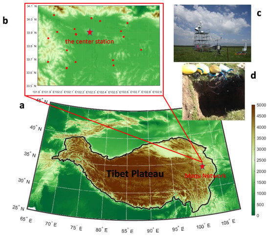
Maqu network is located in the northeast margin of the Tibetan Plateau (Figure 1). The average elevation is about 3300 m above the sea level. The network was built in 2008 and continuously provides soil moisture and soil temperature profile information at 20 sites since then [39]. Since its establishment, the Maqu Network has provided accurate soil moisture and soil temperature measurements for evaluating soil moisture data from satellites [40,41]. The vegetation of the Maqu network consists of meadow and grass less than 1 m in height with roots extending tens of centimeters in depth. An accumulated humus layer of around 10 cm is mixed with the soil. Bushes and trees are scarce in this region, while desert dunes appear along the river off and on. Besides these 20 sites of profile monitoring, there is a complete land-atmosphere interaction observation site which consists of a boundary layer meteorology tower, an eddy covariance system and two dense soil moisture and soil temperature profile measurements.

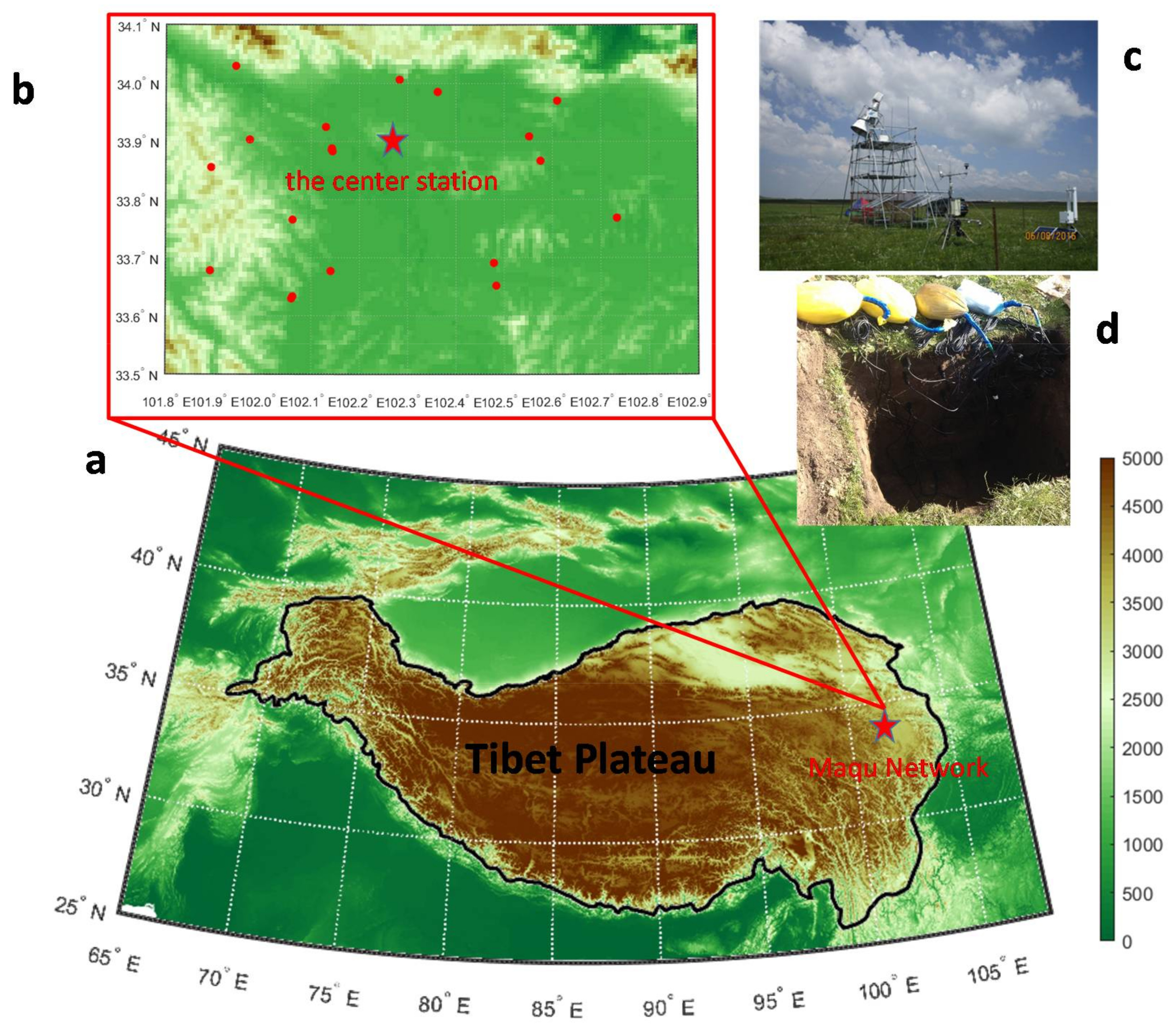
A vertically dense soil moisture and soil temperature profile observation at the center station of Maqu network is used in this study (Figure 1d and Figure 2). To facilitate the comparison with SMAP soil moisture products, the profile data used in this study is provided by ECH20 5TM soil moisture/soil temperature sensors, covering the period from 6 August to 27 November 2016 (Figure 2). It has 20 sensors installed at 19 layers, with two duplicate sensors at 2.5 cm. The depth configuration is illustrated in Figure 2d. Soil moisture data is calibrated with soil texture, bulk density and organic matter content. Furthermore, soil samples are collected near the micro-meteorological observing system, indicating that the soil consists of sand fraction of 26.95% and clay of 9.86% at 0.05 m, respectively, while 29.2% and 10.15% at 0.2 m, 31.6% and 10.43% at 0.4 m [42]. The layer settings for the other sites are 5 cm, 10 cm, 20 cm, 40 cm, and 80 cm or simply 5 cm and 10 cm with an additional infrared sensor for the skin temperature. With such a vertically dense profile observation, we can compute $cc$ for [τ, T] profile at any moment. Mironov’s dielectric constant model was for calculating the real and complex parts of dielectric constants in this study [43].

The in situ data above is used to compute the temporal variation of penetration depth. To extend the understanding of the relationship between soil effective temperature and penetration depth, we also use MERRA-2 (The Modern-Era Retrospective analysis for Research and Applications, Version 2) [44] and SMAP Level 3 radiometer global daily 36 km EASE-Grid soil moisture, Version 4 product in this study to illustrate a spatial distribution of penetration depth. MERRA-2 is supposed to replace former MERRA dataset with the advances made in the assimilation system that enable assimilation of modern hyperspectral radiance and microwave observations, along with GPS-Radio Occultation datasets. The spatial resolution used in this study is 0.625 × 0.5 degree. While soil properties are retrieved from MERRA-2 constant fields, only soil temperature, soil moisture and surface temperature at SMAP over passing time are collected. Since March 2015, SMAP is providing promising global soil moisture distribution with its passive radiometer every 2–3 days [45]. The spatial resolution for passive sensor is 36 km that is double the resolution compared with MERRA-2. In this case, the SMAP L3 product is downscaled with nearest neighbor interpolation method to rebuild the soil moisture map matching with MERRA-2. Since there is just one frequency operated by SMAP, the soil moisture detected should reflect the average emission capacity within a certain depth of soil column, but not a particularly fixed depth. This average soil moisture synthesizes the strong penetration due to longer wavelength at L-band as another virtual concept of $T_{eff}$. As noted in the introduction part, vegetation also affects the penetration depth. In this study, the in situ soil moisture and soil temperature data at Maqu Center Station were used to directly compute the $T_{eff}$ and penetration depth within the soil column, sparing the need to consider the vegetation effect. For SMAP soil moisture product, the impact of vegetation is already removed during the retrieval procedure. It should also be noted that there are other sites at Maqu Network but none of them has vertically dense profile measurement. Without such measurement, the calculated penetration depth strongly depends on the fixed soil moisture layer. In contrast to the SMAP soil moisture product which is derived from average emissivity, the soil moisture at fixed depth is not the same as the average soil moisture. Therefore, it is not appropriate to compute penetration depth for the rest sites at Maqu network.

4. Results

In this section, the penetration depth is first calculated according to Equation (10) for SMOS/SMAP at 1.4 GHz. The result is intended to give a broad view on how penetration depth is affected by soil moisture and soil temperature theoretically. After that, Equation (8) and Equation (11) are applied at Maqu Center Station, where a dedicated penetration depth time series is generated for further analysis. With the penetration depth acquired at Maqu Center Station, we then can select accordingly the soil moisture and soil temperature observation to compare with the integral soil effective temperature by Equation (12).

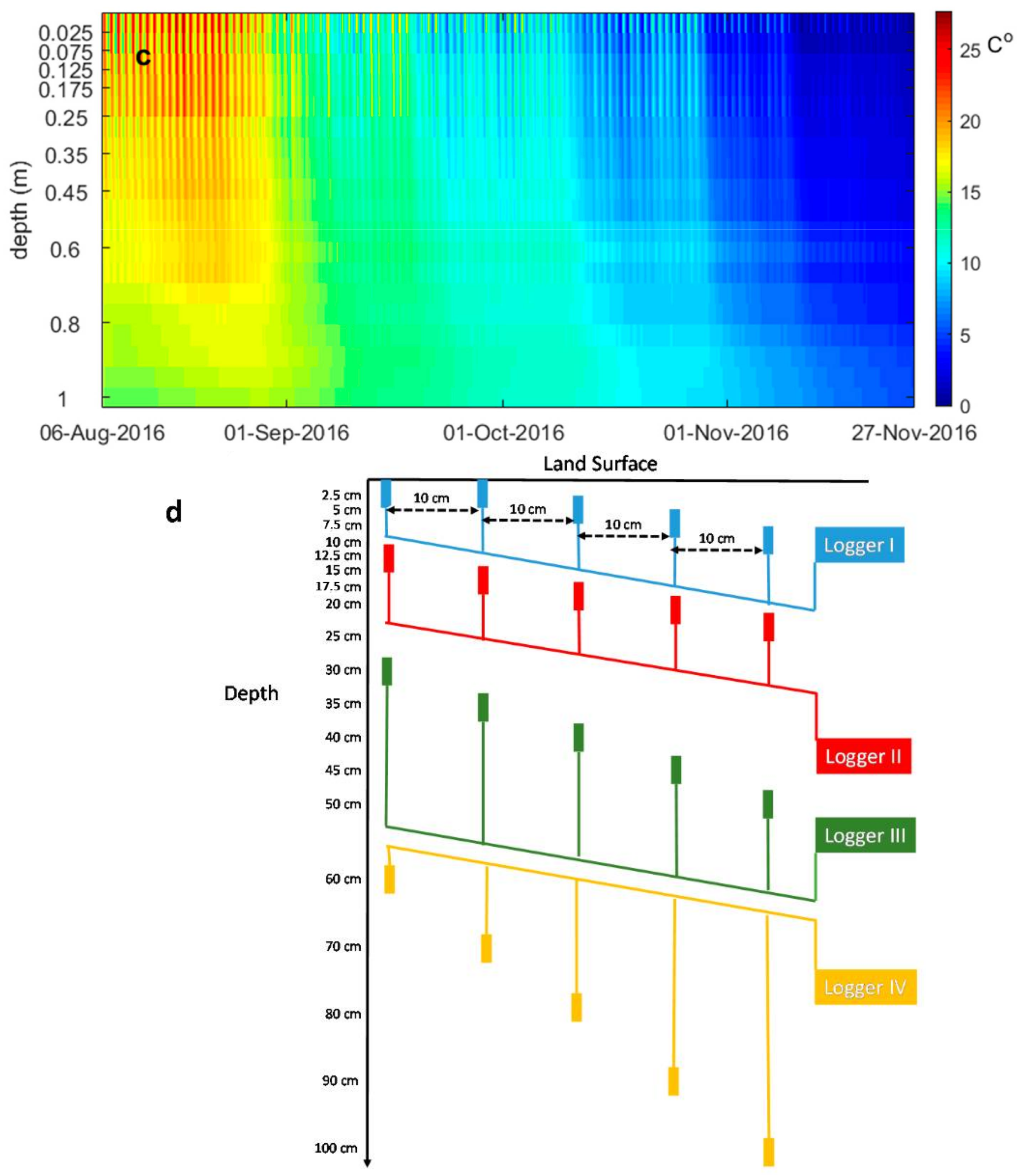
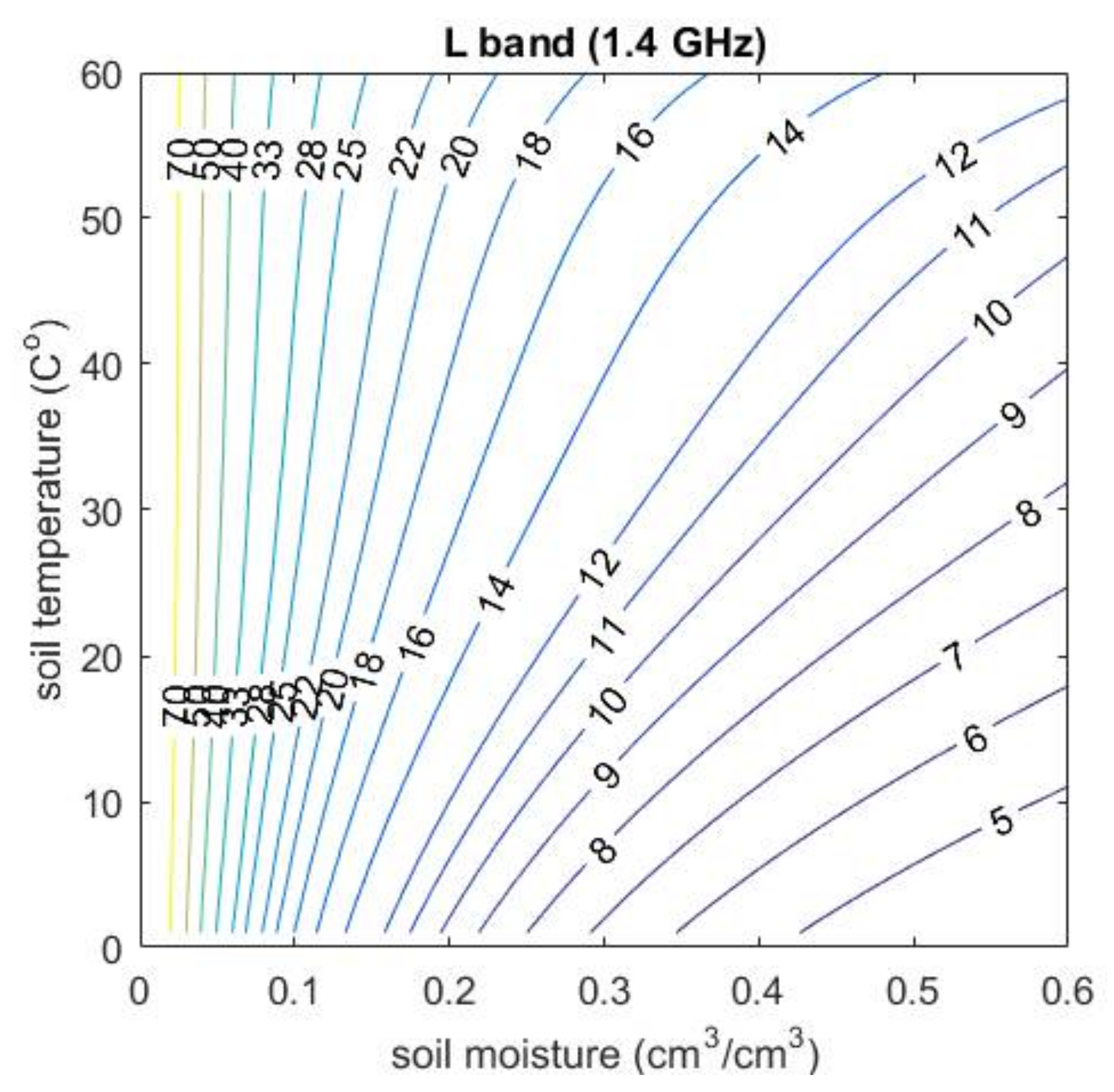
Figure 3 uses the operational channel of SMOS/SMAP (L-band, 1.4 GHz) as examples to show how the soil moisture and soil temperature affect the penetration depth. It is clear that soil moisture is the dominant factor in affecting the penetration depth when the soil is dry, while soil temperature has more impact on the penetration depth for the wet soil. With the range of soil moisture of 0.01–0.6 cm³ cm⁻³ and soil temperature of 0–60 °C, the penetration depth ranges from 3–70 cm for L-band. When the soil is very dry (i.e., soil moisture is less than 0.01 cm³ cm⁻³), the penetration depth is the greatest. Generally, the penetration depth would be 12 cm for L-band at 0.3 cm³ cm⁻³ and 30 °C. If the soil is not so dry, the effect of soil temperature needs to be considered. For instance, in Figure 3, the penetration depth could be 11 cm when soil moisture is 0.55 cm³ cm⁻³ and soil temperature is 50 °C. Nevertheless, the same penetration depth is also associated with soil moisture of 0.2 cm³ cm⁻³ and soil temperature of 10 °C. However, an error of soil temperature both in measurement and model simulation larger than 10 °C is rare and soil moisture dominate the penetration depth especially for dry soil. In this case, although the calculation of the penetration depth strongly depends on the dielectric constant model but the difference can be ignored. If the layers configuration were too sparse, the estimation would not be so precise in practice as in Figure 3. This is partly the reason why a vertically dense soil moisture and soil temperature profile was mounted at the Maqu Center Site with dense layers (19 layers within the top one meter). Such intensive layering would greatly minimize the uncertainty introduced by the dielectric models.

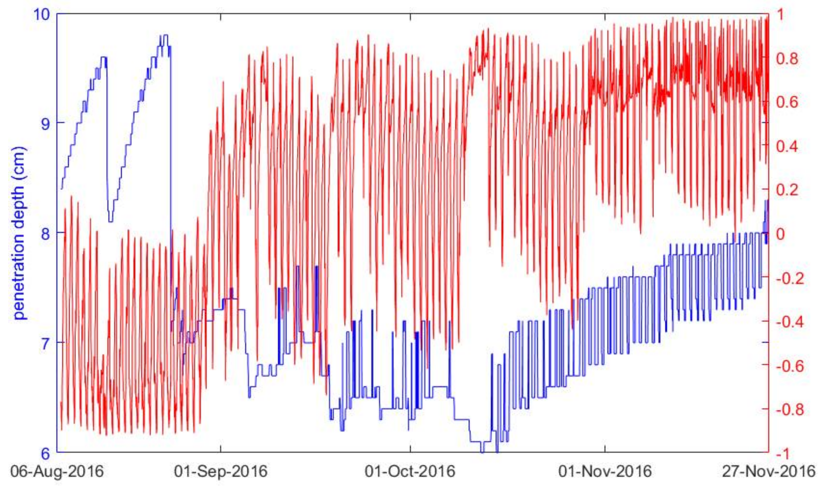
Figure 4 shows the time series of the penetration depth (Blue) and correlation coefficient (Red) between the soil temperature at the penetration depth and the corresponding soil effective temperature. With vertically dense soil moisture/temperature profile measurement at Maqu Center Station, the penetration depth in Figure 4 is computed by Equations (8) and (12). While soil moisture ranges from 0.15 to 0.45 cm³ cm⁻³, the penetration depth varies from 6 to 10 cm at the center site. The average penetration depth is about 9 cm for the time before August 25 and 7 cm for the rest. As can be seen the penetration depth is strongly correlated with soil moisture which explains the variation in the period. Meanwhile, the penetration depth has its diurnal changes (around 1 cm) and is affected dominantly by soil temperature.

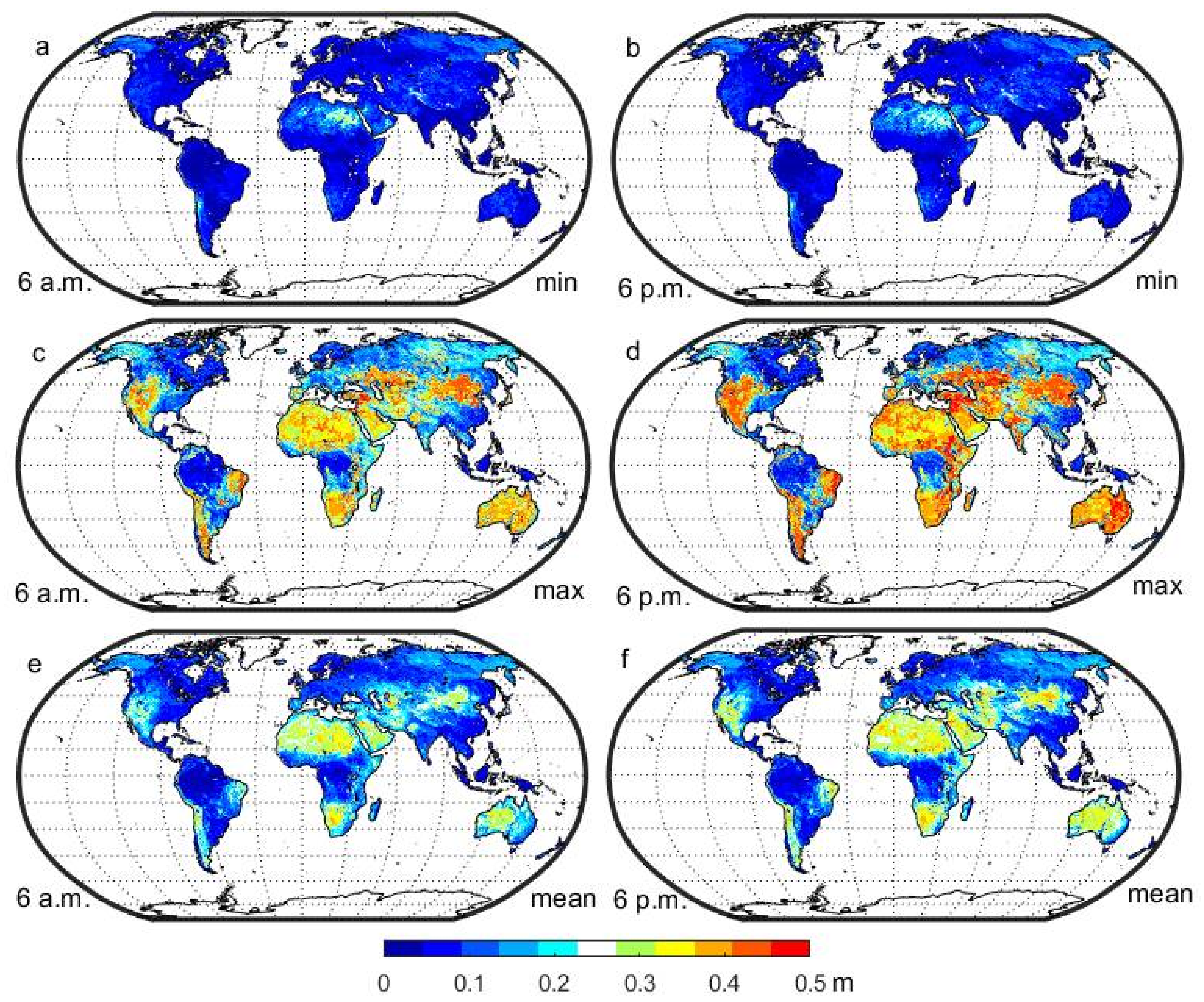
From the foregoing we highlighted the essence of T_eff as the mid-level of soil temperature profile in terms of Equations (1), (5) and (12) which could represent the average soil temperature of the soil column. Similarly, the soil moisture detected by satellites are also supposed to be the average soil moisture of the soil column in the view of emission depth. With T_eff computed from MERRA-2 and global soil moisture map acquired from SMAP, Figure 5 illustrates a global distribution of the penetration depth by Equation (10).

The minimum cases (Figure 5a,b) reflect the penetration depth especially after the rainfall when the soil moisture is then higher. If there is a sufficient rain event, the surface soil layer would be fully moist even the soil column would be dry. Therefore, the penetration depth would be less than 0.1 m or even 0.05 m around the globe. In comparison, the cases for maximum penetration depth (Figure 5c,d) occur after a long drying period when the soil moisture has drawn down from the surface to deeper layers. This situation depends on how dry the soil could be so such regions coincide with the arid regions like central Asia, Australia and Sahara where the penetration depth is over 0.3 m. The annual mean value of penetration depth (Figure 5e,f) is from 0.05 to 0.2 m except the extremely dry regions. According to Equation (7) in Lv’s scheme, the soil moisture/temperature sampled at 0.05 m represents the radiative contribution from 0 m to more than 0.1 m (depending on the specific profile) so 0.05 m samples may match with the satellite signal in most regions. In general, there is not too much difference between 6 a.m. and 6 p.m. while the latter may have deeper penetration depth of a few centimeters because T_eff is higher.

5. Discussion

Because the penetration depth is defined as the depth at which the intensity of the radiation inside the medium reduces to $1/e$ (about 37%) of its original value at the surface (or from its source origin to the surface from a sensing point of view), it means there are about 37% signal comes beneath the penetration depth. To characterize the penetration depth, several factors (see below) need to be considered and their uncertainties quantified, among which the validity of the assumption of linear temperature gradient is of most significance which we will briefly discuss as follows.

Several factors influence the characteristics of penetration depth which means that for Cal/Val the satellite soil moisture product, it is very important to know the overpassing time, because the penetration depth can vary diurnally. On the other hand, Equations (12) and (19) are derived based on the linear assumption (i.e., $\frac{dT}{d\tau }=const$). If the soil moisture and soil temperature profiles are complex or have great gradients, the remotely sensed soil moisture may not be at the penetration depth as calculated by Equation (12).

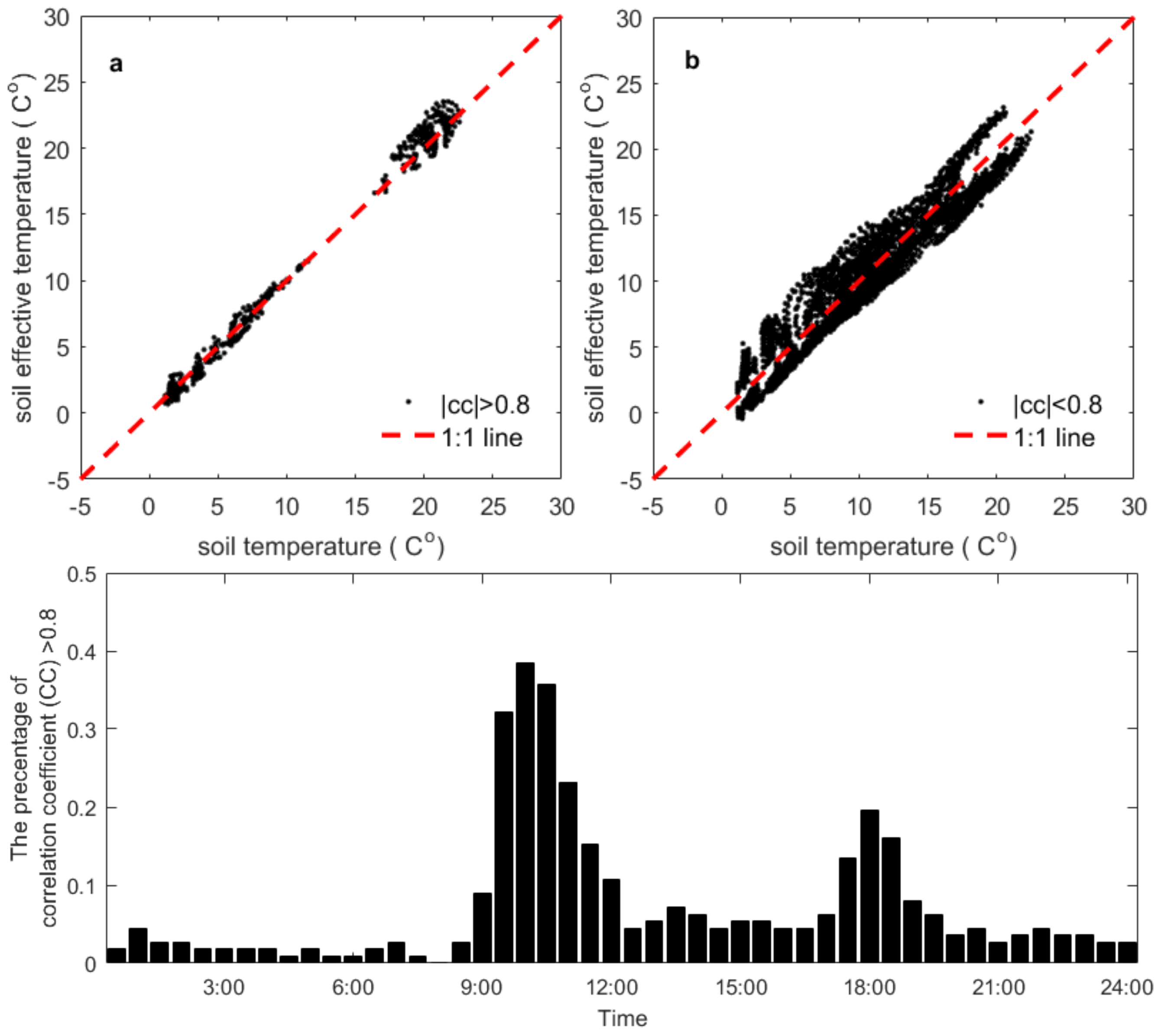
To which extent the linear assumption could be satisfied is quantified by the absolute value of correlation coefficient $\left|cc\right|$ between the soil temperature profile and the optical depth profile at Maqu Center Station. Figure 6 gives a glance about the validity of the linear assumption. It could be seen that the best accuracy was achieved when the assumption is valid if the data satisfy ($\left|cc\right|>0.8$), which accounts for 10.89% during the experiment period. The $\left|cc\right|>0.8$ appears mainly around 10:00 o’clock (local time) and about 40% of the observation period. The second occurrence peak is around 18:00 o’clock (local time) which coincides with SMOS/SMAP descending/ascending overpassing time. Other than the validity of the liner assumption, the assumption of $e^{-{\tau }_{deep}}\approx 0$ in Equation (18) can affect the correlation coefficient as well.

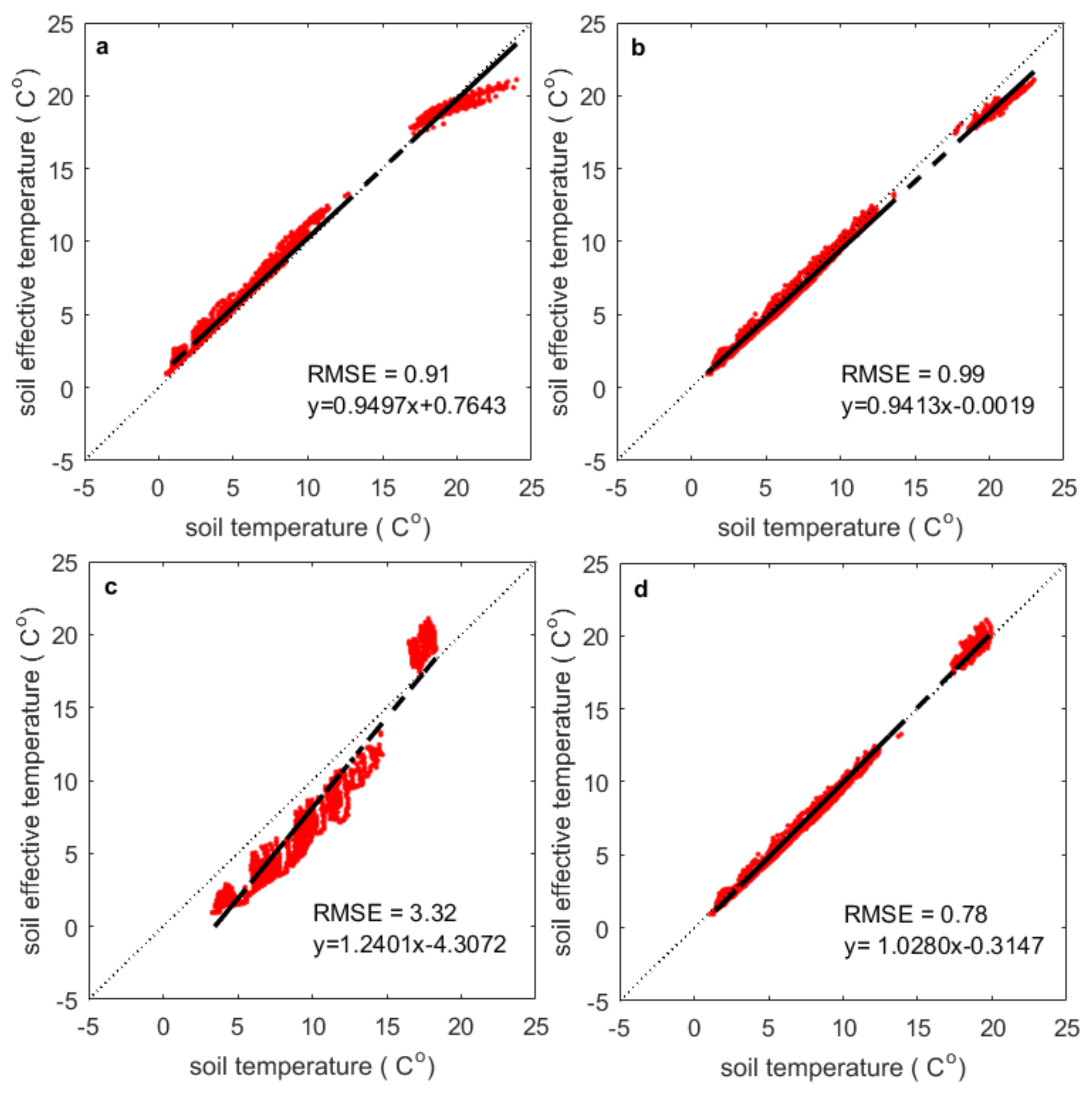
Equation (19) indicates that the soil temperature value at one certain depth could represent the soil temperature profile in terms of soil effective temperature (e.g., Lv’s two-layer scheme vs. Wilheit’s integral scheme) and that depth is the penetration depth. The soil temperature observed at 5 cm, 10 cm, 40 cm and the penetration depth in Figure 4 are compared with the soil effective temperature calculated by Wilheit’s scheme in Figure 7. It is seen that the soil temperature variation at 2.5 cm (Figure 7a) has a slight underestimation bias and the distribution of points is much scattered than at the penetration depth (Figure 7d). For the soil temperature approximately between 15 and 20 °C, the difference can reach about 5 °C. When the soil temperature is out of that temperature range, the difference become relatively smaller. The variation range of soil temperature at 10 cm (Figure 7b) matches better but is still worse than that at the penetration depth. From Figure 4, it is known that the average penetration depth is about 7 cm after 20 August. Therefore the relatively similar accuracy is reasonable between Figure 7b,d. The soil temperature at 40 cm (Figure 7c) has a positive/negative bias after/before 20 August. RMSE reaches 3.32 °C. Obviously 40 cm cannot represent the soil profile (Figure 7c) to calculate T_eff.

For those data with $\left|cc\right|>0.8$ (i.e., $\frac{dT}{d\tau }=\mathit{const}$) (see Figure 6), the soil temperature at the penetration depth is very close to as expected by Equation (19). The penetration depth contains all the factors which affect the soil effective temperature, such that the soil effective temperature varies with the penetration depth.

6. Conclusions

The concept of penetration depth in microwave radiometry was published more than four decades ago and its importance has long been realized by the microwave remote sensing community. The penetration depth is a characteristic length in the soil column which should be considered as a dynamic whole instead of just a few centimeters at the surface layer and becomes especially important with the increased wavelength for the dedicated soil moisture mission SMOS/SMAP. Because the penetration depth is defined based on the integral effective soil temperature, it leaves a gap between the simple two-layer schemes (e.g., commonly used in the operational soil moisture retrieval) and the integral one. Nevertheless, the implication behind the penetration depth has so far not been fully investigated and explained. The casually referred 1/e residual is just a “qualitative” number and how it is linked with satellite soil moisture sensing depth has not been analytically determined.

In this study, with rigorous mathematical derivations based on Lv’s $T_{eff}$ scheme, we have proved that the penetration depth is not only a “qualitative” number but a characteristic depth which synthesizes emitting behavior of a soil column in microwave radiometry. In Lv’s scheme, the optical depth $\tau$ appears in $T_{eff}$ and thus unifies the radiative transfer processes in atmosphere, vegetation and soil. More specifically, $\tau$ quantifies the attenuation of radiation transfer in a medium, being the air dielectric properties in the atmosphere, vegetation optical thickness (mainly the water content in leaves) in vegetation, as well as soil dielectric properties (e.g., mainly soil moisture) in the soil. The use of the integral $\tau$ instead of soil depth $x$ is proposed in this study for the first time and with $\tau$ appearing in the $T_{eff}$ formula, we can determine essential characteristics in $T_{eff}$. By means of $\tau$, it is proved that the penetration is not just the depth where the energy is reduced to 1/e of its original value but it is also the median value of soil temperature in the soil column. The penetration depth is strongly related to soil moisture but also has diurnal variation which may have an amplitude of several centimeters at the center station of Maqu network.

The question of at which depth L-band soil moisture monitoring satellites such as SMOS/SMAP measure has confused the soil moisture community at large. As stated in introduction, the sensitive layer is supposed to be the depth where these satellites are sensing in previous studies. In SMAP retrieval [46], vegetation and soil surface roughness are accounted in terms of emissivity calibration. The final soil moisture product is derived from a smooth emission model. A precise estimation of vegetation and roughness is critical before determining the penetration depth. Particularly, the global map of penetration depth in Figure 5 depends on a correct vegetation calibration. Therefore, the penetration depth over dense vegetation zone, for instance the tropics may be even smaller. In contrast, in the dessert area with few or no vegetation, the penetration depth is usually large and vegetation calibration is not so important except after rainfall events. The conclusion in this study would be most useful to the transition zone where soil moisture variation is larger and affects climate/hydro-process more intensively. Different to the sensitive layer view, we proposed in this study a median value view and found the soil temperature median value under the linear assumption. From the hypothesis of zeroth-order incoherent microwave transfer frame, the median soil temperature layer represents not only $T_{eff}$ but also provides the depth information contained in this frame. The soil moisture retrieved from microwave (e.g., L-band) observation should be the average radiative emission capacity of the soil column and there should be a median soil moisture depth as well. This study has successfully developed such a new method to find this median soil moisture depth by relating the penetrating depth in terms of temperature to radiative energy attenuation. This is done by building up a $T_b\sim T_{eff}\sim \tau \sim depth$ relationship with median theory in which a median value of $T$ could be found at the penetration depth with certain condition. The method is verified with in situ data from the Maqu observation site and the conclusion is valid whenever the field condition satisfies the assumption. This is critical to the application of SMOS/SMAP soil moisture product because a difference of several centimeters between the depth of in situ measurement and the satellite sensing depth will lead to systematic bias in evaluating the satellite products. Based on an application of the developed method to SMAP passive L3 soil moisture product and the corresponding soil effective temperature calculated from MERRA-2 for 2016, it may be concluded that it is appropriate to use 5 cm depth of soil moisture measurement as a ground reference to calibrate and validate satellites soil moisture product because 5 cm captures the main signal source on average. However, for some extreme cases like arid region or the region after a long drought event, 5 cm may not represent the dominant emission layer. In other words, it means that even though the satellite product is precise, we may still get biased conclusion, if the ground measurement is inappropriately organized, and the comparability between satellite and in situ measurement is not established [47]. The developed method should also be beneficial to the Earth surface modelling in improving the consistency in the dynamics of the soil moisture processes and satellite observations.

References

- Yamada, T.J.; Kanae, S.; Oki, T.; Hirabayashi, Y. The onset of the West African monsoon simulated in a high-resolution atmospheric general circulation model with reanalyzed soil moisture fields. Atmos. Sci. Lett. 2012, 13, 103–107. [Google Scholar] [CrossRef]
- Douville, H.; Chauvin, F.; Broqua, H. Influence of soil moisture on the Asian and African monsoons. Part I: Mean monsoon and daily precipitation. J. Clim. 2001, 14, 2381–2403. [Google Scholar] [CrossRef]
- Douville, H.; Conil, S.; Tyteca, S.; Voldoire, A. Soil moisture memory and West African monsoon predictability: Artefact or reality? Clim. Dyn. 2007, 28, 723–742. [Google Scholar] [CrossRef] [Green Version]
- Lim, Y.J.; Hong, J.; Lee, T.Y. Spin-up behavior of soil moisture content over East Asia in a land surface model. Meteorol. Atmos. Phys. 2012, 118, 151–161. [Google Scholar] [CrossRef]
- De Rosnay, P.; Drusch, M.; Boone, A.; Balsamo, G.; Decharme, B.; Harris, P.; Kerr, Y.; Pellarin, T.; Polcher, J.; Wigneron, J.P. AMMA land surface model intercomparison experiment coupled to the Community Microwave Emission Model: ALMIP-MEM. J. Geophys. Res. Atmos. 2009, 114. [Google Scholar] [CrossRef]
- Kerr, Y.H. Soil moisture from space: Where are we? Hydrogeol. J. 2006, 15, 117–120. [Google Scholar] [CrossRef]
- Dedieu, G.; Deschamps, P.Y.; Kerr, Y.H. Satellite estimation of solar irradiance at the surface of the Earth and of surface albedo using a physical model applied to meteosat data. J. Clim. Appl. Meteorol. 1987, 26, 79–87. [Google Scholar] [CrossRef]
- Kerr, Y.H.; Waldteufel, P.; Richaume, P.; Wigneron, J.P.; Ferrazzoli, P.; Mahmoodi, A.; Al Bitar, A.; Cabot, F.; Gruhier, C.; Juglea, S.E.; et al. The SMOS soil moisture retrieval algorithm. IEEE Trans. Geosci. Remote Sens. 2012, 50, 1384–1403. [Google Scholar] [CrossRef]
- Entekhabi, D.; Njoku, E.G.; O’Neill, P.E.; Kellogg, K.H.; Crow, W.T.; Edelstein, W.N.; Entin, J.K.; Goodman, S.D.; Jackson, T.J.; Johnson, J.; et al. The Soil Moisture Active Passive (SMAP) Mission. Proc. IEEE 2010, 98, 704–716. [Google Scholar] [CrossRef]
- Dumedah, G.; Walker, J.P.; Rudiger, C. Can SMOS data be used directly on the 15-km discrete global grid? IEEE Trans. Geosci. Remote Sens. 2014, 52, 2538–2544. [Google Scholar] [CrossRef]
- Reul, N.; Tenerelli, J.; Chapron, B.; Vandemark, D.; Quilfen, Y.; Kerr, Y. SMOS satellite L-band radiometer: A new capability for ocean surface remote sensing in hurricanes. J. Geophys. Res. Oceans 2012, 117. [Google Scholar] [CrossRef]
- Dente, L.; Su, Z.B.; Wen, J. Validation of SMOS soil moisture products over the Maqu and Twente regions. Sensors 2012, 12, 9965–9986. [Google Scholar] [CrossRef] [PubMed]
- Tranchant, B.; Testut, C.E.; Renault, L.; Ferry, N.; Birol, F.; Brasseur, P. Expected impact of the future SMOS and Aquarius Ocean surface salinity missions in the Mercator Ocean operational systems: New perspectives to monitor ocean circulation. Remote Sens. Environ. 2008, 112, 1476–1487. [Google Scholar] [CrossRef]
- Tranchant, B.; Testut, C.E.; Ferry, N.; Renault, L.; Obligis, E.; Boone, C.; Larnicol, G. Data assimilation of simulated SSS SMOS products in an ocean forecasting system. J. Oper. Oceanogr. 2008, 1, 19–27. [Google Scholar] [CrossRef]
- Lv, S.; Zeng, Y.; Wen, J.; Zheng, D.; Su, Z. Determination of the optimal mounting depth for calculating effective soil temperature at l-band: Maqu case. Remote Sens. 2016, 8, 476. [Google Scholar] [CrossRef]
- Lv, S.; Wen, J.; Zeng, Y.; Tian, H.; Su, Z. An improved two-layer algorithm for estimating effective soil temperature in microwave radiometry using in situ temperature and soil moisture measurements. Remote Sens. Environ. 2014, 152, 356–363. [Google Scholar] [CrossRef]
- Burke, W.J.; Schmugge, T.; Paris, J.F. Comparison of 2.8- and 21-cm microwave radiometer observations over soils with emission model calculations. J. Geophys. Res. Oceans 1979, 84, 287–294. [Google Scholar] [CrossRef]
- Rao, K.; Chandra, G.; Rao, P.N. Study on penetration depth and its dependence on frequency, soil moisture, texture and temperature in the context of microwave remote sensing. J. Indian Soc. Remote Sens. 1988, 16, 7–19. [Google Scholar] [CrossRef]
- Njoku, E.G.; Kong, J.-A. Theory for passive microwave remote-sensing of near-surface soil-moisture. J. Geophys. Res. 1977, 82, 3108–3118. [Google Scholar] [CrossRef]
- Colliander, A.; Jackson, T.J.; Bindlish, R.; Chan, S.; Das, N.; Kim, S.B.; Cosh, M.H.; Dunbar, R.S.; Dang, L.; Pashaian, L.; et al. Validation of SMAP surface soil moisture products with core validation sites. Remote Sens. Environ. 2017, 191, 215–231. [Google Scholar] [CrossRef]
- Su, Z.; de Rosnay, P.; Wen, J.; Wang, L.; Zeng, Y. Evaluation of ECMWF’s soil moisture analyses using observations on the Tibetan Plateau. J. Geophys. Res. Atmos. 2013, 118, 5304–5318. [Google Scholar] [CrossRef]
- Njoku, E.G.; Entekhabi, D. Passive microwave remote sensing of soil moisture. J. Hydrol. 1996, 184, 101–129. [Google Scholar] [CrossRef]
- Entekhabi, D.; Nakamura, H.; Njoku, E.G. Solving the inverse problems for soil-moisture and temperature profiles by sequential assimilation of multifrequency remotely-sensed observations. IEEE Trans. Geosci. Remote Sens. 1994, 32, 438–448. [Google Scholar] [CrossRef]
- Escorihuela, M.J.; Chanzy, A.; Wigneron, J.P.; Kerr, Y.H. Effective soil moisture sampling depth of L-band radiometry: A case study. Remote Sens. Environ. 2010, 114, 995–1001. [Google Scholar] [CrossRef] [Green Version]
- Scheeler, R.; Kuester, E.F.; Popovic, Z. Sensing depth of microwave radiation for internal body temperature measurement. IEEE Trans. Antennas Propag. 2014, 62, 1293–1303. [Google Scholar] [CrossRef]
- Zhou, F.C.; Song, X.N.; Leng, P.; Li, Z.L. An effective emission depth model for passive microwave remote sensing. IEEE J. Sel. Top. Appl. Earth Obs. Remote Sens. 2016, 9, 1752–1760. [Google Scholar] [CrossRef]
- Nolan, M.; Fatland, D.R. Penetration depth as a DInSAR observable and proxy for soil moisture. IEEE Trans. Geosci. Remote Sens. 2003, 41, 532–537. [Google Scholar] [CrossRef]
- Zhao, S.; Zhang, L.; Zhang, T.; Hao, Z.; Chai, L.; Zhang, Z. An empirical model to estimate the microwave penetration depth of frozen soil. In Proceedings of the 2012 IEEE International Geoscience and Remote Sensing Symposium (IGARSS), Munich, Germany, 22–27 July 2012; pp. 4493–4496. [Google Scholar]
- Choudhury, B.J.; Schmugge, T.J.; Mo, T. A Parameterization of Effective Soil-Temperature for Microwave Emission. J. Geophys. Res. Oceans 1982, 87, 1301–1304. [Google Scholar] [CrossRef]
- Wigneron, J.P.; Laguerre, L.; Kerr, Y.H. A simple parameterization of the L-band microwave emission from rough agricultural soils. IEEE Trans. Geosci. Remote Sens. 2001, 39, 1697–1707. [Google Scholar] [CrossRef]
- Holmes, T.R.H.; de Rosnay, P.; de Jeu, R.; Wigneron, R.J.P.; Kerr, Y.; Calvet, J.C.; Escorihuela, M.J.; Saleh, K.; Lemaitre, F. A new parameterization of the effective temperature for L band radiometry. Geophys. Res. Lett. 2006, 33. [Google Scholar] [CrossRef]
- Ulaby, F.T.; Moore, R.K.; Fung, A.K. Microwave Remote Sensing Active and Passive-Volume III: From Theory to Applications; Artech House, Inc.: Norwood, MA, USA, 1986. [Google Scholar]
- Lv, S.; Zeng, Y.; Wen, J.; Su, Z. A reappraisal of global soil effective temperature schemes. Remote Sens. Environ. 2016, 183, 144–153. [Google Scholar] [CrossRef]
- De Rosnay, P.; Wigneron, J.; Holmes, T.; Calvet, J. Parameterizations of the effective temperature for L-band radiometry. Inter-comparison and long term validation with SMOSREX field experiment. In Thermal Microwave Radiation-Applications for Remote Sensing; IET Electromagnetic Waves Series 52; Mtzler, C., Rosenkranz, P.W., Battaglia, A., Wigneron, J.P., Eds.; Christian Matzler: London, UK, 2006; Volume 573, ISBN 0-86341-573-3 and 978-086341-573-9. [Google Scholar]
- Wilheit, T.T. Radiative-transfer in a plane stratified dielectric. IEEE Trans. Geosci. Remote Sens. 1978, 16, 138–143. [Google Scholar] [CrossRef]
- Zwieback, S.; Hensley, S.; Hajnsek, I. Assessment of soil moisture effects on L-band radar interferometry. Remote Sens. Environ. 2015, 164, 77–89. [Google Scholar] [CrossRef] [Green Version]
- Owe, M.; Van de Griend, A.A. Comparison of soil moisture penetration depths for several bare soils at two microwave frequencies and implications for remote sensing. Water Resour. Res. 1998, 34, 2319–2327. [Google Scholar] [CrossRef] [Green Version]
- Wigneron, J.P.; Chanzy, A.; de Rosnay, P.; Rudiger, C.; Calvet, J.C. Estimating the effective soil temperature at L-band as a function of soil properties. IEEE Trans. Geosci. Remote Sens. 2008, 46, 797–807. [Google Scholar] [CrossRef]
- Su, Z.; Wen, J.; Dente, L.; van der Velde, R.; Wang, L.; Ma, Y.; Yang, K.; Hu, Z. The Tibetan Plateau observatory of plateau scale soil moisture and soil temperature (Tibet-Obs) for quantifying uncertainties in coarse resolution satellite and model products. Hydrol. Earth Syst. Sci. 2011, 15, 2303–2316. [Google Scholar] [CrossRef]
- Zheng, D.; Wang, X.; van der Velde, R.; Zeng, Y.; Wen, J.; Wang, Z.; Schwank, M.; Ferrazzoli, P.; Su, Z. L-band microwave emission of soil freezesc-thaw process in the Third Pole Environment. IEEE Trans. Geosci. Remote Sens. 2017. [Google Scholar] [CrossRef]
- Wang, Q.; van der Velde, R.; Su, Z. Use of a discrete electromagnetic model for simulating Aquarius L-band active/passive observations and soil moisture retrieval. Remote Sens. Environ. 2017, 205, 434–452. [Google Scholar] [CrossRef]
- Zhao, H.; Zeng, Y.; Lv, S.; Su, Z. Analysis of soil hydraulic and thermal properties for land surface modelling over the tibetan plateau. Earth Syst. Sci. Data Discuss. 2018. [Google Scholar] [CrossRef]
- Mironov, V.L.; Dobson, M.C.; Kaupp, V.H.; Komarov, S.A.; Kleshchenko, V.N. Generalized refractive mixing dielectric model for moist soils. IEEE Trans. Geosci. Remote Sens. 2004, 42, 773–785. [Google Scholar] [CrossRef]
- Gelaro, R.; McCarty, W.; Suárez, M.J.; Todling, R.; Molod, A.; Takacs, L.; Randles, C.A.; Darmenov, A.; Bosilovich, M.G.; Reichle, R.; et al. The Modern-Era Retrospective Analysis for Research and Applications, Version 2 (MERRA-2). J. Clim. 2017, 30, 5419–5454. [Google Scholar] [CrossRef]
- O’Neill, P.; Chan, S.; Njoku, E.; Jackson, T.; Bindlish, R. Soil Moisture Active Passive (SMAP), Algorithm Theoretical Basis Document Level 2 & 3 Soil Moisture (Passive) Data Products, Revison B; Jet Propulsion Laboratory, California Institute of Technology: Pasadena, CA, USA, 2015. [Google Scholar]
- Entekhabi, D.; Yueh, S.; O’Neill, P.E.; Kellogg, K.H.; Allen, A.; Bindlish, R.; Brown, M.; Chan, S.; Colliander, A.; Crow, W.T. SMAP Handbook—Soil Moisture Active Passive: Mapping Soil Moisture and Freeze/Thaw from Space; National Aeronautics and Space Administration (NASA): Washington, DC, USA, 2014.
- Zeng, J.; Li, Z.; Chen, Q.; Bi, H.; Qiu, J.; Zou, P. Evaluation of remotely sensed and reanalysis soil moisture products over the Tibetan Plateau using in-situ observations. Remote Sens. Environ. 2015, 163, 91–110. [Google Scholar] [CrossRef]
Figure 1.
(a) Geographical location of the Maqu network on the Tibetan Plateau. The background indicates the elevation from USGS 1 km topography and the border in black is where elevation >2500 m; (b) The distribution of all sites at the Maqu network and the center site (ELBARA) located in the center; (c) ELABRA; (d) the detailed soil moisture and soil temperature profile.
Figure 2.
(a) precipitation; (b) the time series of soil moisture and (c) soil temperature profiles at Maqu Network Center Station; (d) the installation configuration of 20 sensors.
Figure 3.
Penetration depth at L band (1.4 GHz). The ranges of penetration depth (in centimeters) were shown as contour lines, depending on the soil moisture and soil temperature. Mironov’s dielectric constant model was used here for calculating the real and complex parts of dielectric constants.
Figure 4.
The time series of the penetration depth (Blue) and correlation coefficient (Red) between the soil temperature at the penetration depth and the corresponding soil effective temperature at Maqu Center Station as computed from the soil temperature/moisture profiles between 6 August and 27 November 2016.
Figure 5.
Global map of the penetration depth (PD) for SMAP with (a) minimum at 6 a.m.; (b) minimum at 6 p.m.; (c) maximum at 6 a.m.; (d) maximum at 6 p.m.; (e) mean at 6 a.m.; (f) mean at 6 p.m. Data used are SMAP soil moisture passive L3 product and the corresponding soil effective temperature calculated from MERRA-2 for 2016. The SMAP soil moisture and soil effective temperature are considered as the mid-level values for each pixel vertically.
Figure 6.
Comparison of soil temperature at the penetration depth vs. soil effective temperature at Maqu Center Station. The absolute correlation coefficient () divided the time series into two groups where (a) and (b). The bottom figure shows the daily distribution of the moment when correlation coefficient .
Figure 7.
Comparison of soil effective temperature calculated by Wilheit’s integral scheme against soil temperature observed at Maqu Center Station: (a) 2.5 cm; (b) 10 cm; (c) 40 cm observation and (d) the penetration depth. Data are shown only when and the dashed line is the regression line. The period is from 6 August to 27 November 2016.