Color Enhancement for Four-Component Decomposed Polarimetric SAR Image Based on a CIE-Lab Encoding

Abstract

Color enhancement of decomposed fully polarimetric synthetic aperture radar (PolSAR) image is vital for visual understanding and interpretation of the polarimetric information about the target. It is common practice to use RGB or HIS color space to display the chromatic information for polarization-encoded, Pauli-basis images, or model-based target decomposition of PolSAR images. However, to represent the chroma for multi-polarization SAR data, the region of basic RGB color space does not fully cover the human perceptual system, leading to information loss. In this paper, we propose a color-encoding framework based on the CIE-Lab, a perceptually uniform color space, aiming at a better visual perception and information exploration. The effective interpretability in increasing chromatic, and thus visual enhancement, is presented using extensive datasets. In particular, the four decomposed components—volume scattering, surface scattering, double bounce, and helix scattering—along with total return power, are simultaneously mapped into the color space to improve the discernibility among the scattering components. The five channels derived from the four-component decomposition method can be simultaneously mapped to CIE-Lab color space intuitively. Results show that the proposed color enhancement not only preserves the color tone of the polarization signatures, but also magnifies the target information embedded in the total returned power.

1. Introduction

Color enhancement for different bands or polarization channels is powerful for analyzing the elements within an image pixel by the human eye. Color encoding has been extensively used in multispectral remote sensing data [1,2,3]. Some advanced color-coding techniques to exploit visually exploit PolSAR imagery, in both polarization and temporal channels. Examples include using the adaptive processing (MAP3) to enhance interpretation for multi-temporal data [4], and the enhance MAP3 to deal with coherency window size for multi-temporal SAR data [5]. For example, image classification by measuring the color differences in optical multispectral remote sensing data using CIE-Lab color space was suggested in [6]. Color encoding was also designed in mapping the polarization information to retain their qualitative features in an effort of detecting targets in scattering media [7]. Mapping of Poincare sphere to CIE-Lab color space using polarization stokes vector with four elements and segmentation using fuzzy C-means technique was presented in [8]. However, a question generally raised is what kind of color coding scheme is best or optimally suited for a particular context or objective in a general image domain.

However, much less attention is paid to exploring a suitable color enhancement for target decomposition in fully polarimetric synthetic aperture radar (PolSAR) data to improve the visual interpretation and hence exploit the full power of polarization signature for target classification, detection, and identification. Target decomposition of a PolSAR image is a powerful tool to characterize the terrain features. It is useful to interpret the scattering mechanisms by applying model-based decomposition techniques [9,10,11,12,13]. In four-component decomposition [12,13], for example, a simple RGB is commonly used in mapping three components, double bounce, volume, and surface scattering, and the fourth component, helix scattering, is independently displayed in grayscale, or simply by heuristic color mixing. This at least causes some degree of difficulty for inclined viewers. It was indicated that in RGB color space, with the absence of the helix scattering component, the total power of the three elements combined is unable to maintain the consistency. The power of four-component decomposition is not fully presented in pseudo-color image space. Clearly, to counter this drawback, what is need is a proper color transformation that maps the four components into a consistent color space while preserving their individual and unique features. The basic idea is to give color composition without losing much of the information offered by target decomposition. For visual inspection and interpretation, a simple way is to display individual components monotonically. Color mapping, if properly devised, could better convey the target information through spatial, spectral, and polarized signatures in decomposed components. For this reason, it is recognized that color enhancement is vital because the human eye cannot discern the polarization signature effectively. Basically, there are three criteria [3] that must be satisfied for a chosen color enhancement scheme:

• The discrimination of the variables that represent the specific scattering attribute is essential.
• The temporal or spatial variation by movement of targets is stood out more effectively.
• The reparability in controlling brightness and chromatic expansion can enhance the legibility.

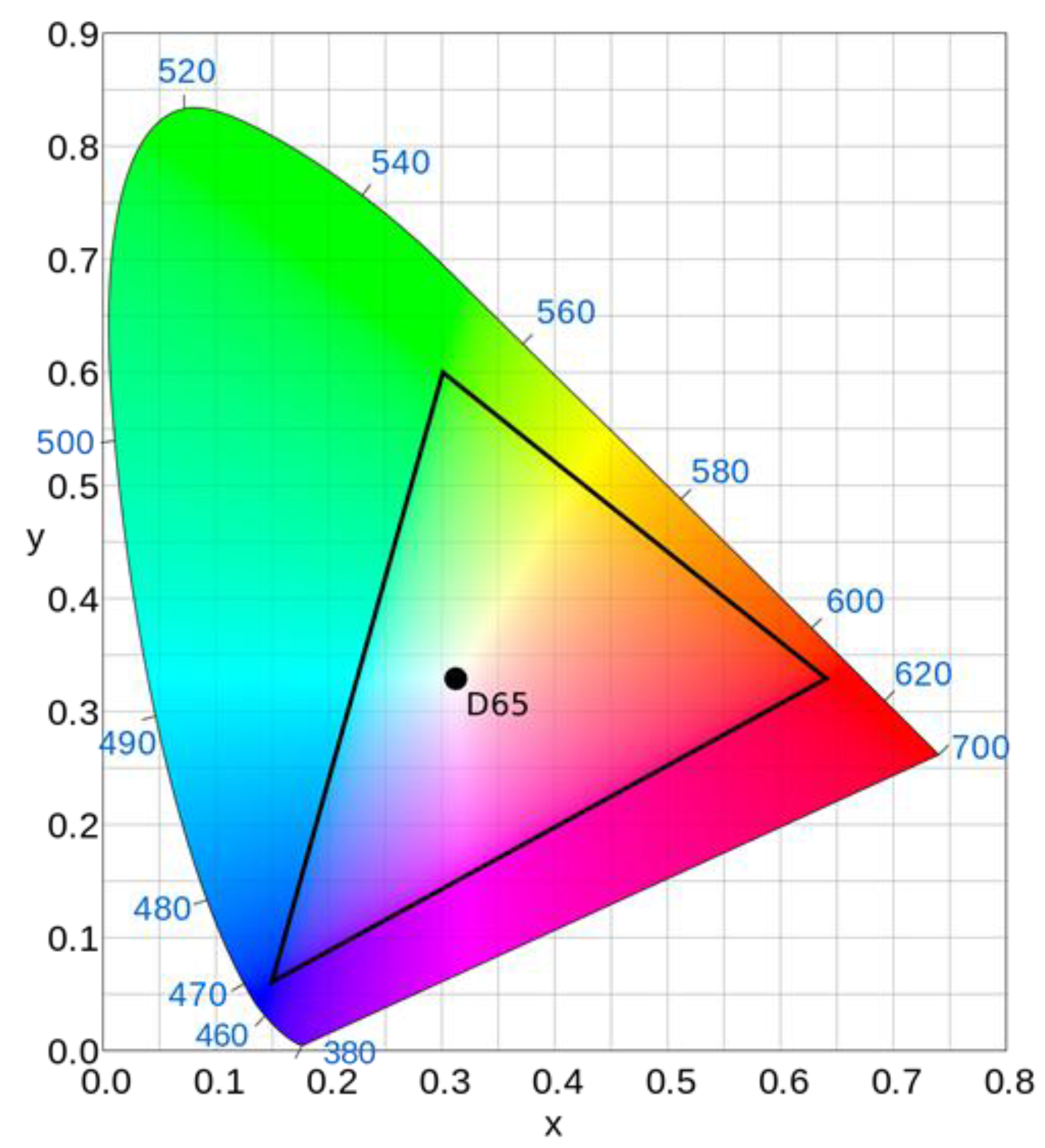
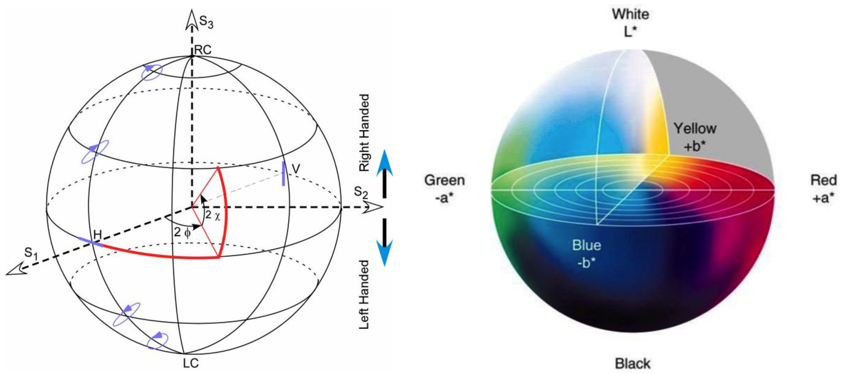
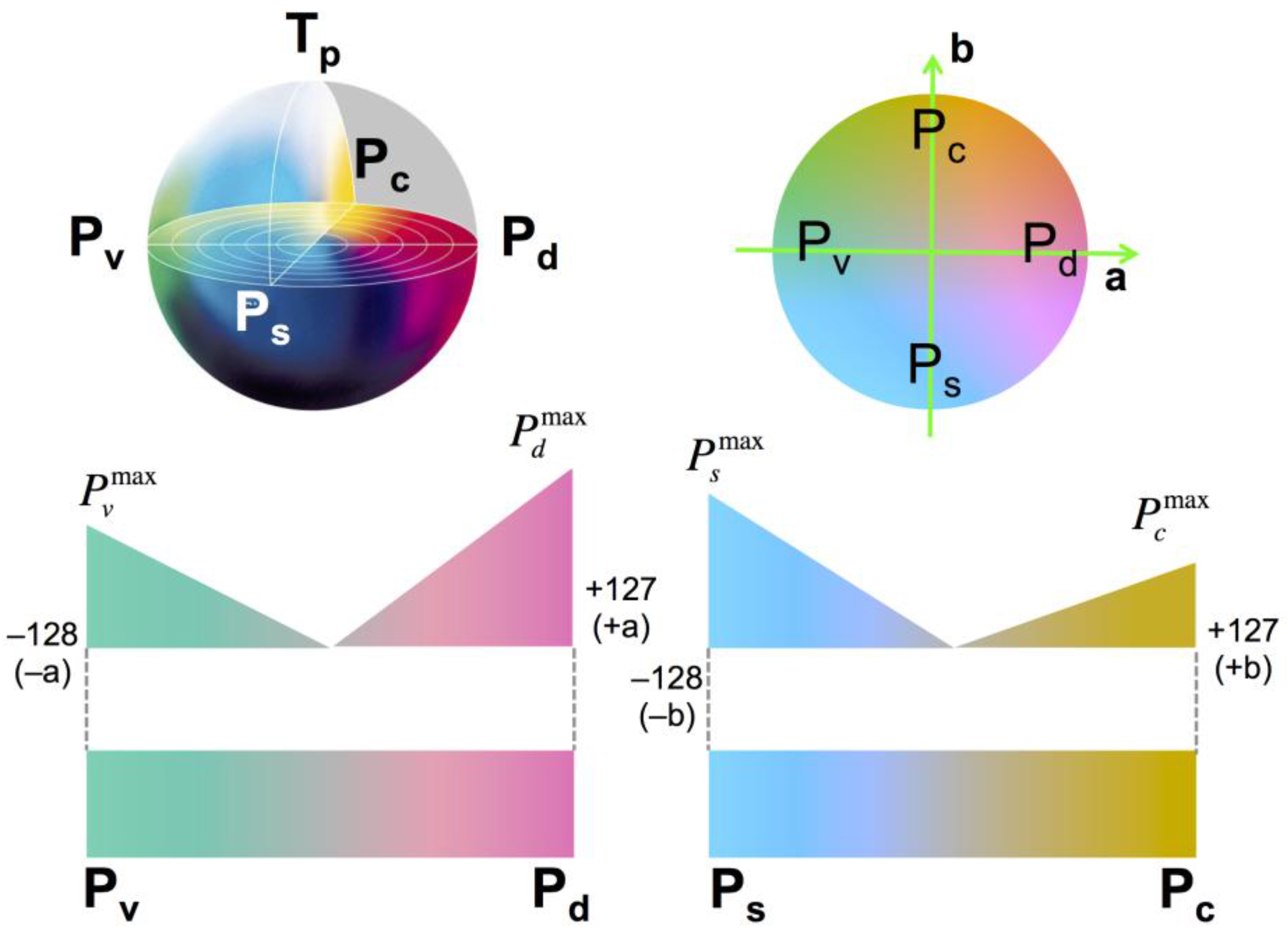
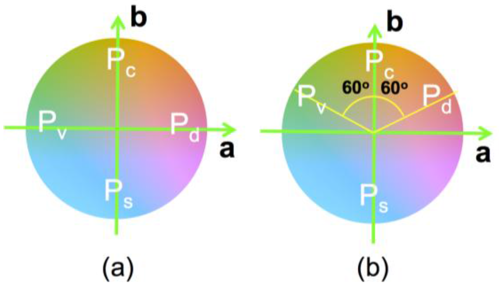
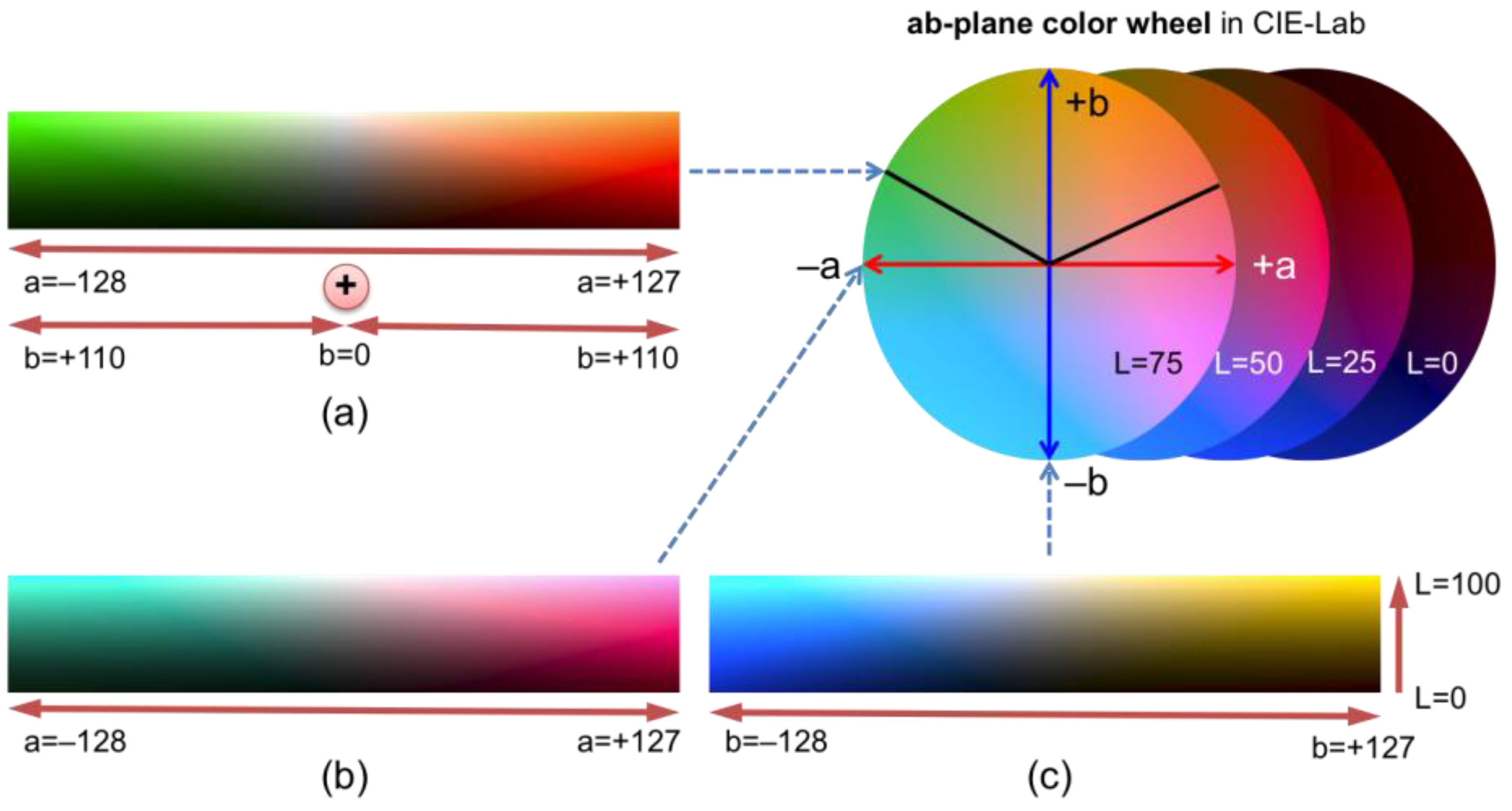
Following the above three guidelines, in PolSAR image visualization, the main objective of color enhancement is to explore the capability of quantitative and qualitative detection or classification for objects of mixed scattering mechanism in PolSAR image. We establish a framework for assignment of fully polarization data decomposed by Yamaguchi’s four-component decomposition with rotation using the power of uniform perceptual CIE-Lab color space, such that not only is the chroma by four components preserved, but the total power to enhance the target structure is conceived.

The organization of this paper is as follows. In the next section, we give the rationale for CIE-Lab color space being chosen for polarization data. The uniform perceptual color assignment, CIE-Lab color space, and the framework of transformation from information data to display device monitor are discussed in Section 2. A proper coding scheme for PolSAR image is proposed and the procedure is thoroughly described and outlined in Section 3. Section 4 presents the experimental results and discussions. Finally, conclusions and future directions are drawn from this study to close the paper.

2. Color Space

Several definitions of RGB, such as Adobe RGB 1998, CIE RGB, ProPhoto RGB, among others, [14,15] are commonly used. The objective of the definition of RGB is to fit the color range of a human visual system, as presented in the CIE 1964 xy chromaticity diagram in Figure 1.

As shown in Figure 1, not only the color temperature (referred to as the white point) but also the three primaries must be determined, and hence the boundary of this basic color space, the triangular area within the figure, is rather restricted compared to those in naked eye. RGB colors cannot cover and lie within the whole region. In contrast to basic color space, RGB or CYMK, which is determined by the displayer or monitor, the general CIE-Lab color space is specifically designed to match human visual perception. The perceptually uniform color space, such as CIE-Lab or CIE-Luv, is combined with illumination, chroma, and hue-angle in general. The illumination is closely connected with the human perception of lightness. The separability of brightness and chroma satisfies the three principles. The CIE-Lab color space, to which is allocated the white point, covers a larger area of the color gamut than the basic color space.

3. Color Enhancement for Decomposed PolSAR Images

In total, five channels of data are generated, including total power channels (as known as SPAN) in Yamaguchi’s four-component decomposition with rotation [12,13], known as Y4R. The four components include volume, double bounce, surface, and helix scattering, each exhibiting different behavior of scattering mechanisms, while the total power channel retains not only the geometrical properties of the target being observed, but also dielectric information on the medium. This closely resembles the multispectral and panchromatic data formation and spectral property in optical data. In SAR polarimetry, the Stokes parameters may be mapped onto the Poincare sphere to completely describe all polarization states. The perceptually uniform color space such as CIE-Lab is combined by illumination, and chroma with hue-angle generally [16,17], in which the illumination is closely connected with the human perception of light. The CIE-Lab color space is colorimetric and perceptually uniform [17]. Hence, it is intuitive to map the polarization signature in CIE-Lab color space, which defines a, b (the value between −128 and +127) and brightness axis L (between 0 and 100) with respective to the xyz-axis in Cartesian coordinates, where a extends from turquoise to rose, and b from blue to yellow. Note that all values are in 16 bits half-precision floating-point. Referring to Figure 2, we may assign the total power to the brightness axis to represent the target’s structure and thus to enhance the contrast of the boundary.

Essentially, two steps are involved: the first is mapping from PolSAR data space onto perceptually uniform color space with respect to the four-component decomposition channels and CIE-Lab color space; and the second is enhancing the optional transformation between the perceptually uniform and device-dependent color spaces. Note that, because the conversion in stage two is non-linear, the loss of certain colors in the difference of gamut area is inevitable, and irreversible. A detailed description is given below.

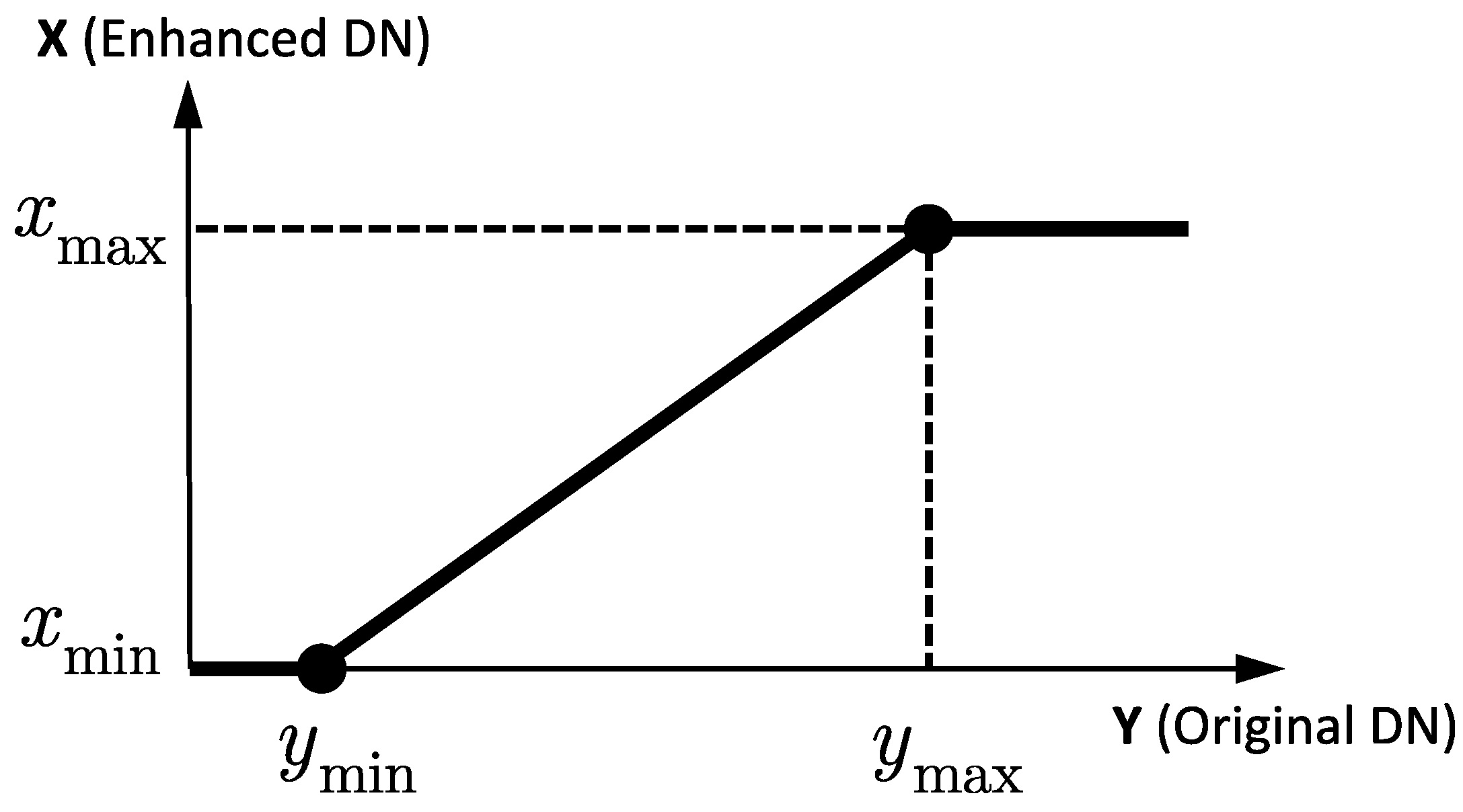
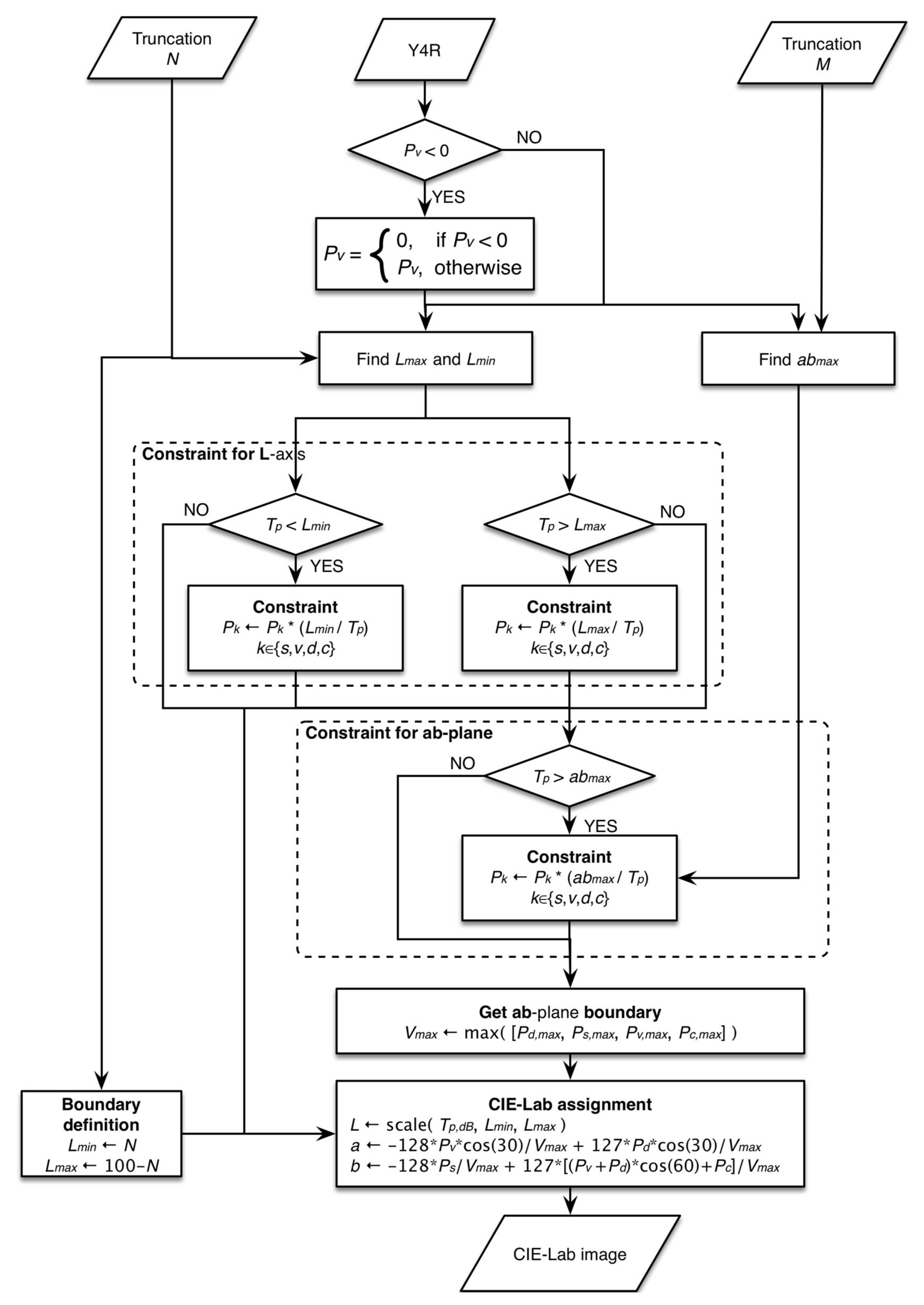
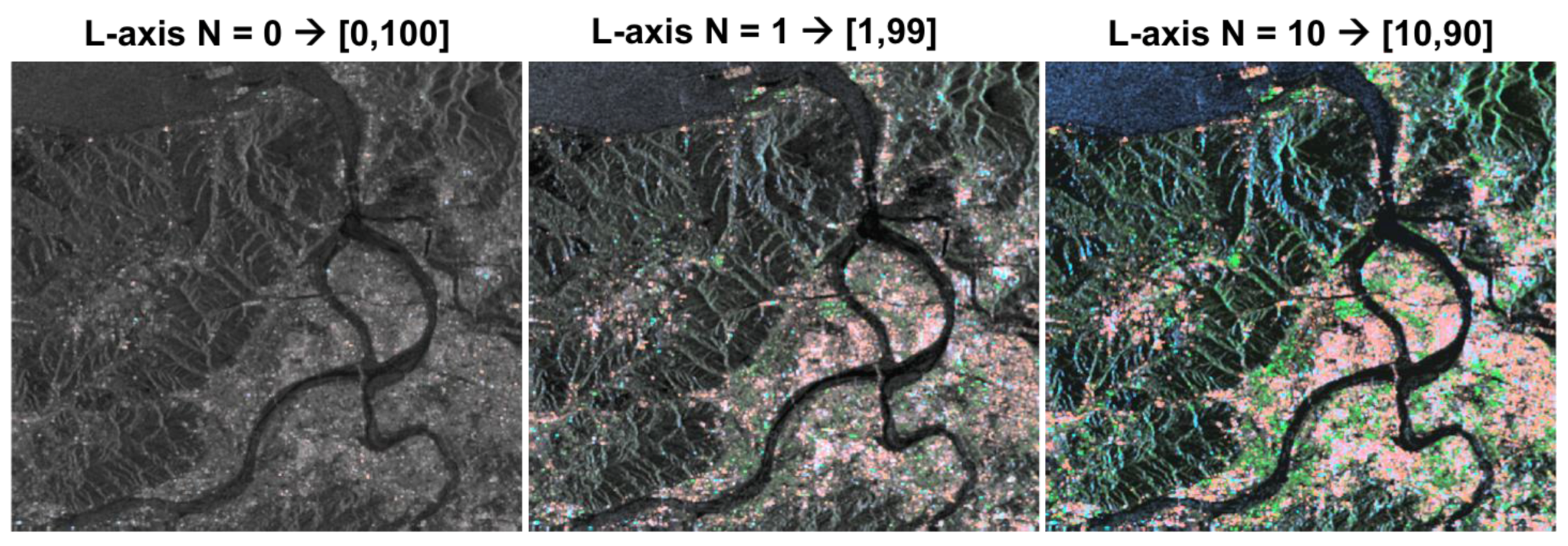
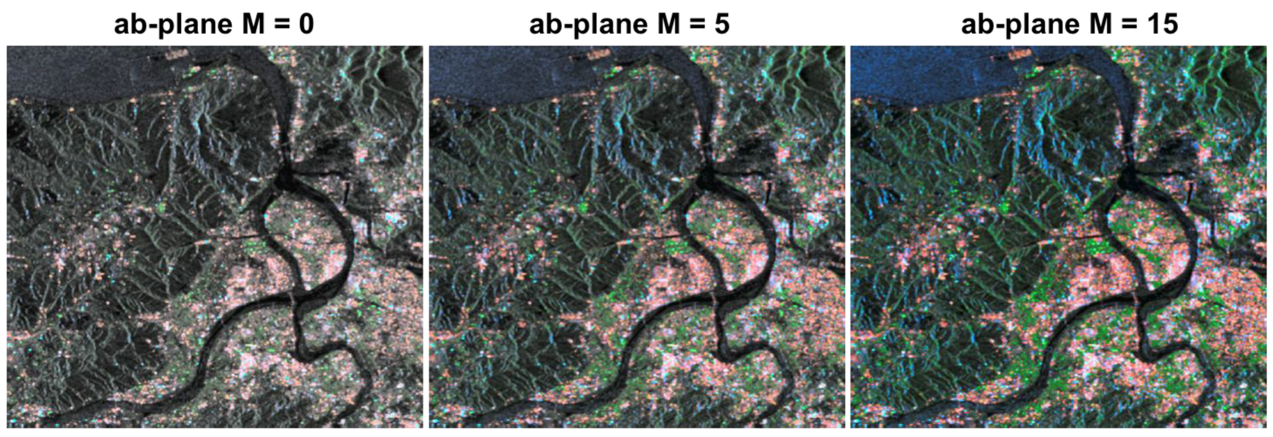
3.1. Data Slicing as Preprocessing

Due to the presence of isolated strong targets, image enhancement using histogram equalization or contrast stretching is a common practice [16]. In this paper, in order to keep the data intake as much as possible, we apply simple data slicing to the total. Suppose that the original data y with normalized digital number (DN) (between 0 and 1) has a probability density function. If 2N%, N% for the lower bound and another N% for the upper bound, of the data is to be sliced for the purpose of enhancement, then the local minimum $y_{\min }$ and the local maximum $y_{\max }$ are determined from a cumulative distribution function F, where

$$F(y_{\min })=N/100$$

(1)

$$F(y_{\max })=(1-N)/100.$$

(2)

After determining the local minimum $y_{\min }$ and the local maximum $y_{\max }$ for a preselected slicing percentage, it is now necessary to map the sliced data into enhanced data through a linear mapping function as illustrated in Figure 3, where the original data now range from $y_{\min }$ to $y_{\max }$, from which the corresponding enhanced DN values $x$ can be expressed as

$$x=\{\begin{array}{c}{x}_{\min },if y<y_{\min }\\ x_{\max },if y>y_{\max }\\ \left(\frac{x_{\max }-x_{\min }}{y_{\max }-y_{\min }}\right)\left(y-y_{\min }\right)+x_{\min },otherwise\end{array},x\in X,y\in Y.$$

(3)

In Equation (3), y and x represent four channels, original and enhanced, respectively, that constrain the new minimal and maximal boundary by normalizing the total power. $x_{\min }$ and $x_{\max }$ define the enhanced DN boundary. For example, they will be −128 and +128 to satisfy the a- or b-axis range in the CIE-Lab definition. We illustrate the effects in the following subsections.

3.2. Mapping from PolSAR Data to Perceptually Uniform Color Space

Now the next step is to designate the four decomposition components in CIE-Lab color space such that the target information can be strongly and yet effectively brought out for visual analysis. To begin with, let us linearly assign the volume scattering to a negative value and double bounce scattering to a positive value in the a-axis; and in the b-axis the surface and helix scattering components are assigned to negative and positive values, respectively, followed by formulating the linear combination for chroma of CIE-Lab color space, taking into account the perceptually uniform property. It is implied that the distance in two different colors on the color wheel in certain illumination is similar to the Euclidean geometry distance.

Figure 4 schematically illustrates the assignment of four scattering components in CIE-Lab color space, taking the dynamic range of each component into account. The volume scattering Pv starts with green, while the double bounce Pd starts from red; similarly, the surface scattering Ps begins with blue and ends the helix scattering Pc with yellow. Such an assignment allows the four scattering components to be accommodated into a single color space, enabling easy discernibility. Notice that the total power is mapped onto the brightness axis L.

It is worth noting that in coding in CIE-Lab color space, color re-alignment may be made to a scattering component of interest. The idea is to ensure the weaker scattering component can be properly represented in color space without leaving it behind. When it comes to coding in CIE-Lab color space, it is possible to align the channel of main interest to the a axis while rotating the other channels away from the b axis. In Figure 5a, we see that the pairs P_v–P_d, P_s–P_c are aligned with the a and b axis, respectively. Indeed, we might keep one pair alignment fixed, while adjusting the other pair out of a or b axis. For example, in order to enhance a weaker scattering component, e.g., helix scattering, we turn P_v and P_d 30 degrees away from the a axis, but keep P_s–P_c aligned with the b axis, as shown in Figure 5b. Another option is to suppress the scattering component if it is of no interest. From this example, we also see that coding in CIE-Lab space offers large flexibility, contingent upon users’ inclinations and objectives.

Notice that because the helix scattering, P_c, is relatively weak, it is assigned in yellow and located in the positive b-axis, as shown in Figure 5b. In practice, because the color tone shifts to blue, green, and magenta, we rotate the P_v and P_d components by 30 degrees from the a-axis so that the composite color image shifts toward the warm color. In so doing, mixing the helix component with those rotations thus balances the entire color image between cool and warm tones. After a 30-degree rotation from the a-axis, the color mixes to pistachio (warm green) and vermilion (warm red) at the two ends, as shown in Figure 6a. Figure 6b,c shows the symmetrical color along the a- and b-axis with the different L values progressively. The ends of the negative and positive a-axis are turquoise (cold green) and rose (cold red), respectively, in CIE-RGB color space. The b-axis is similar to the a-axis and the end position is blue and yellow. Effects of rotation angles using the profile will be illustrated in examples later.

Based on the above coding scheme and rules, the mathematical expressions for color assignment take the form

$$\begin{array}{l}L\triangleq scale\left(T_{p,dB},L_{\min },L_{\max }\right)\\ a\triangleq -128\frac{P_v\cos {30}^{\mathrm{o}}}{V_{\max }}+127\frac{P_d\cos {30}^{\mathrm{o}}}{V_{\max }}\\ b\triangleq -128\frac{P_s}{V_{\max }}+127\frac{\left(P_v+P_d\right)\cos {60}^{\mathrm{o}}+P_c}{V_{\max }}\\ \mathrm{where}\\ V_{\max }\triangleq \max \left(\left[P_{d,\max },P_{s,\max },P_{v,\max },P_{c,\max }\right]\right)\end{array}$$

(4)

where $T_{p,dB}$ is the total power component in dB, $T_p$, in dB; scale(⋅) a linear function that scales $T_{p,dB}$ into between $L_{\min },L_{\max }$, determined by user-defined slicing percentage, 2N%. The normalization factor, $V_{\max }$, is defined as the global maximum value among the four scattering components; $P_{d,\max }$, $P_{s,\max }$, $P_{v,\max }$ and $P_{c,\max }$ represent the local maxima of respective components. The ratio of each component, after normalization, can therefore be consistently retained. This is imperative in visual interpretation. To further enrich the saturation and brightness tones, and simultaneously fuse the total power information, color enhancement in CIE-Lab is implemented. The flow chart in Figure 7 explains the detailed steps.

To start with, the volume scattering component is set to zero if its value is negative and the other three components remain unchanged. In CIE-Lab color space, enhancement can be done either in L-axis or ab-plane, or both. Hence the constraint boundary in L-axis and ab-plane should be defined. Let $L_{\min }$ and $L_{\max }$ denote the minimum and maximum levels of the total power histogram by 2N% for L-axis enhancement, leading to the total power being within $[L_{\min },L_{\max }]$, as given in Equation (4). In the ab-plane, we only need to constraint the upper bound, M%, which gives a threshold such that when the total power value exceeds $a{b}_{\max }$, values in the ab-plane are rescaled. The saturation of the image will be higher when the value of M% increases. This means that the sample data in the ab-plane are stretched linearly to two ends of color and the near gray level values in the center of the color bar. If the normalized total power is beyond the two boundaries, the four scattering components are renormalized to ensure the normalized total power equals the boundary values. Note that the treatment of the negative power problem is only from a color mapping point of view. Physical and statistical treatment of the negative power problem in Y4R target composition can be found in [18,19]. Lee et al. [20] proposed algorithms to mitigate the deficiency of negative power that occurred in model-based target decomposition and found that the number of occurrences of negative power was significantly reduced.

Figure 8 shows the L-axis slicing values of 2N%, with N equal to to 0, 1, and 10, where N = 0 indicates the mapping to the overall L-axis without enhancement. When N increases, it is expected that the strong scattering points will be eliminated and the detailed target structures will be lost. The range of mapping L-axis can be adjusted, by changing N, while retaining the dynamic range of the total power. The color tone is tilted forward to low saturation with slightly lower N values. For a predefined boundary, M%, low saturation points extend to near the end of the axis, representing more saturation color. The effects of tuning the M value in the ab-plane are shown in Figure 9, where M values are set from zero to 15% for the case of N = 1. For the best visual effect, after extensive trial and error, setting M to 15 for ab-plane slicing in total power was suggested.

4. Experiment Results and Discussion

To demonstrate the effectiveness and performance of the proposed color enhancement scheme, extensive PolSAR imagery data are tested.

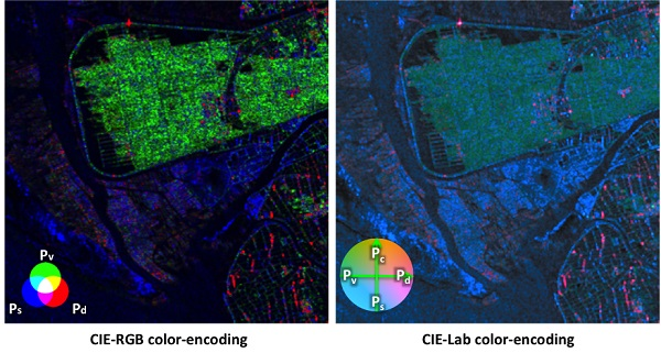
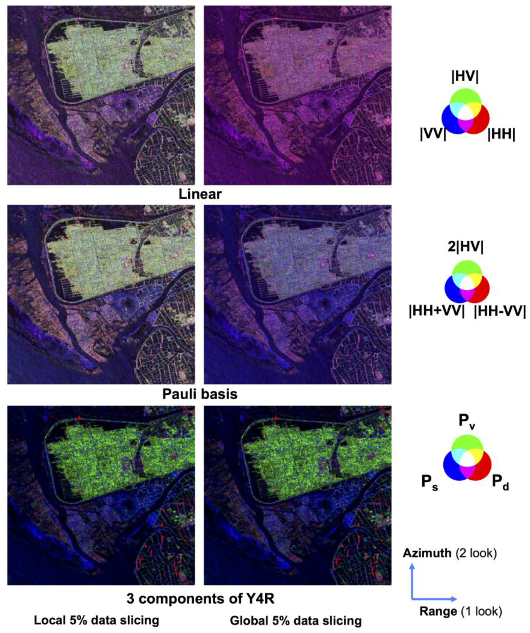
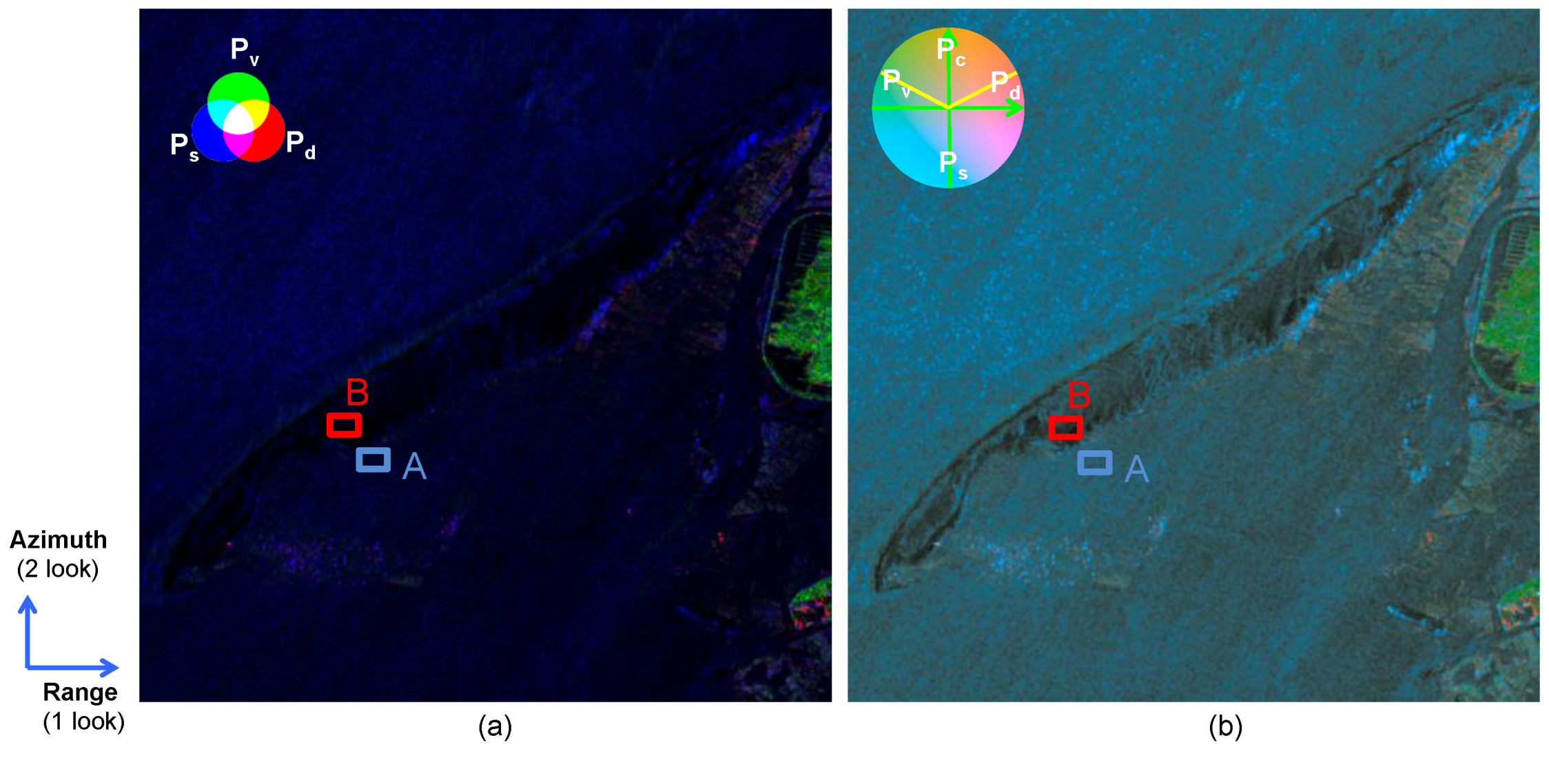
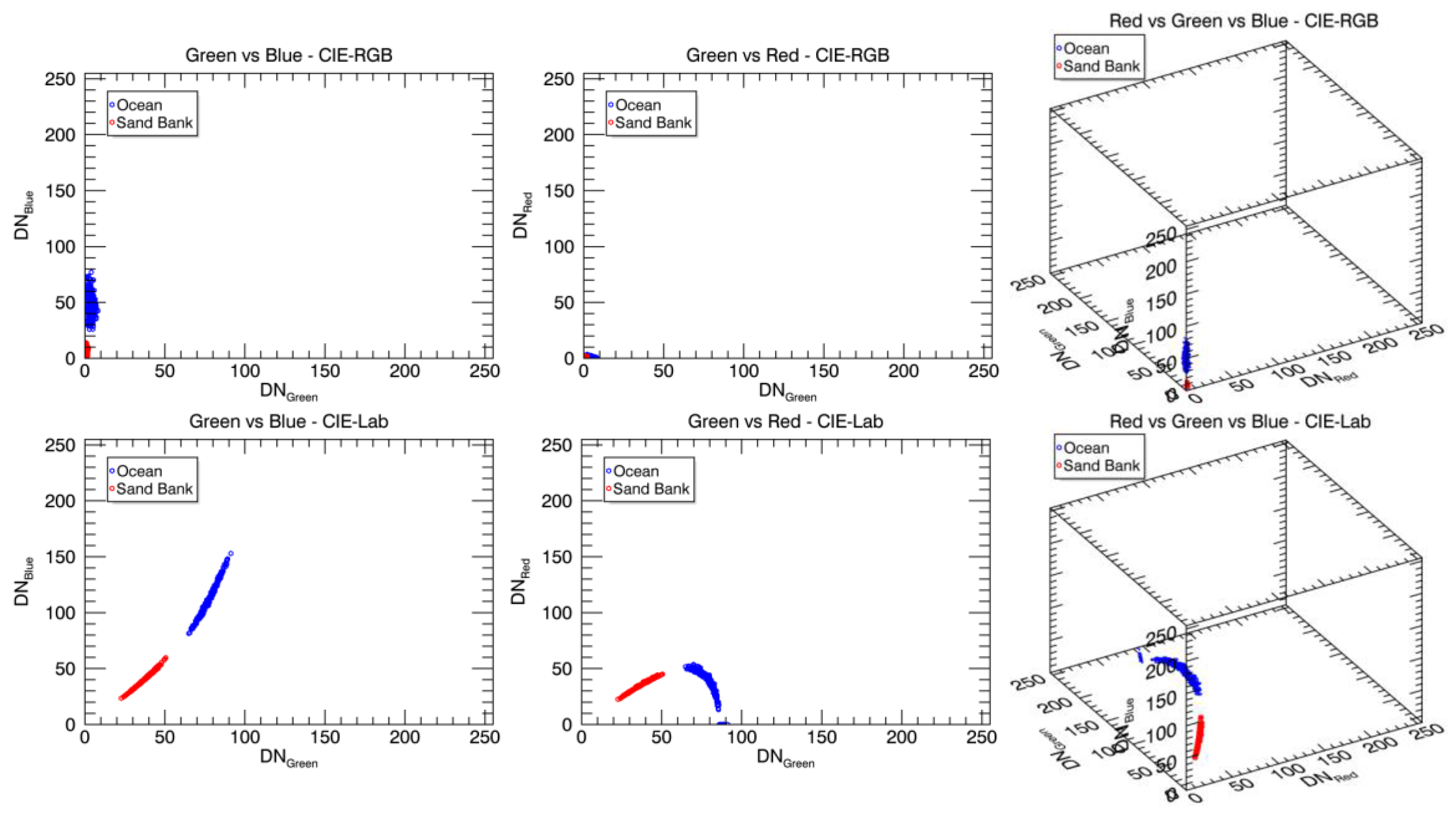
4.1. RGB Color Space

The first test image is the Rasarsat-2 data acquired on 3 June 2012 at fine quad polarization mode with nominal 6 m of spatial resolution. For comparison, we first display the RGB color composition given in Figure 10, which shows the color composition for three linearly polarized channels, HH, VV, and HV (known as lexicographic basis), Pauli basis, and three decomposed components of Y4R, with local and global data slicing of 5% data. Here the local data slicing means that each channel is enhanced by local minimum and maximum values. On the other hand, the overall data ranges within all channels are sliced globally. It is easy to compare the pros and cons of color enhancement by two slicing on local and global basis. With the local slicing, the visual reorganization can be significantly improved but somehow loses the identifiability of different color channels. Results clearly reveal that in CIE-RGB space, the visualization effect is highly sensitive to the choice of data slicing. We will not discuss it further but instead turn our attention to CIE-Lab color mapping.

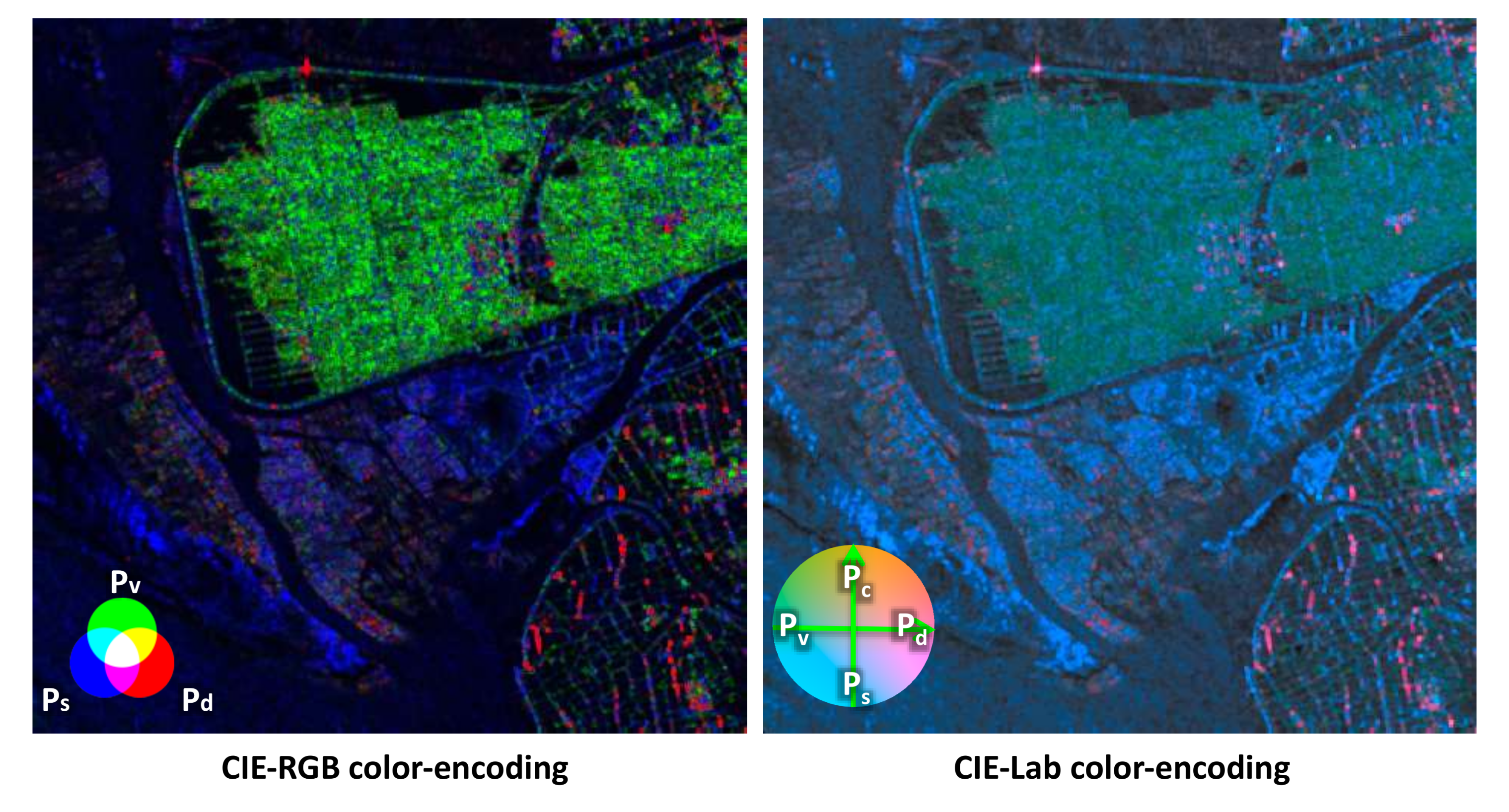
4.2. CIE—Color Space

Figure 11 displays the linear mapping of the four scattering components of Y4R in CIE-Lab color space, where the CIE-RGB result is also included for the purposes of comparison. It is seen that in CIE-RGB color space, the reddish patches (left middle and lower center regions) overwhelmingly stood out along the coast. From the ground truth, these regions were oyster farms, which are geometrically vertical structures. With CIE-Lab color-encoding, the reddish patterns are enhanced more by including the helix component. Note that the total power is reflected in the brightness of the color image, enabling it to reveal richer target information. Nevertheless, we can observe that the tone could be biased in favor of blue and green colors in this image. This is because the helix scattering component is relatively weak compared to volume, surface, and double-bounce scattering components in this image scene, as suggested by ground truth work conducted in time of image taken.

Figure 12 compares the color display with different alignments of components. By doing so, we rotate the surface and double-bounce scattering components in the color wheel. The effect of doing this is to make volume scattering stand out. A strong double-bounce scattering (shown in the upper middle) is noted as the more yellowish region since we rotate the P_d component 60 degrees away from the a-axis (Figure 12a). Similarly, we can keep the surface scattering component aligned but rotate P_v and P_d toward green and red, respectively, and then adjust the double and volume scattering by 30 degrees from the a-axis, as shown in Figure 12b. In Figure 12c, the three components are rotated in the color wheel to preserve and enhance the helix component. It is seen that with coding in CIE-Lab color space, the color contrast can be used to enhance the subtle difference between the two scattering components. Usually, it is desirable to differentiate the variations of total power within the same scattering component. In CIE-Lab color space, it is easy to accommodate four scattering components along with the total power by simply making P_s–P_c alignment (Figure 12c).

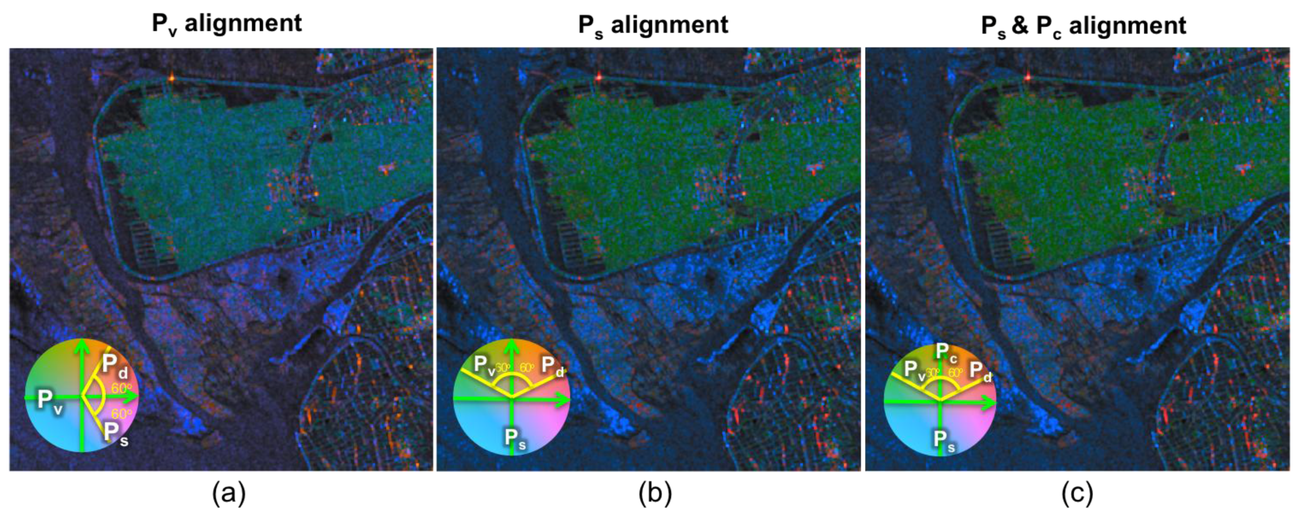
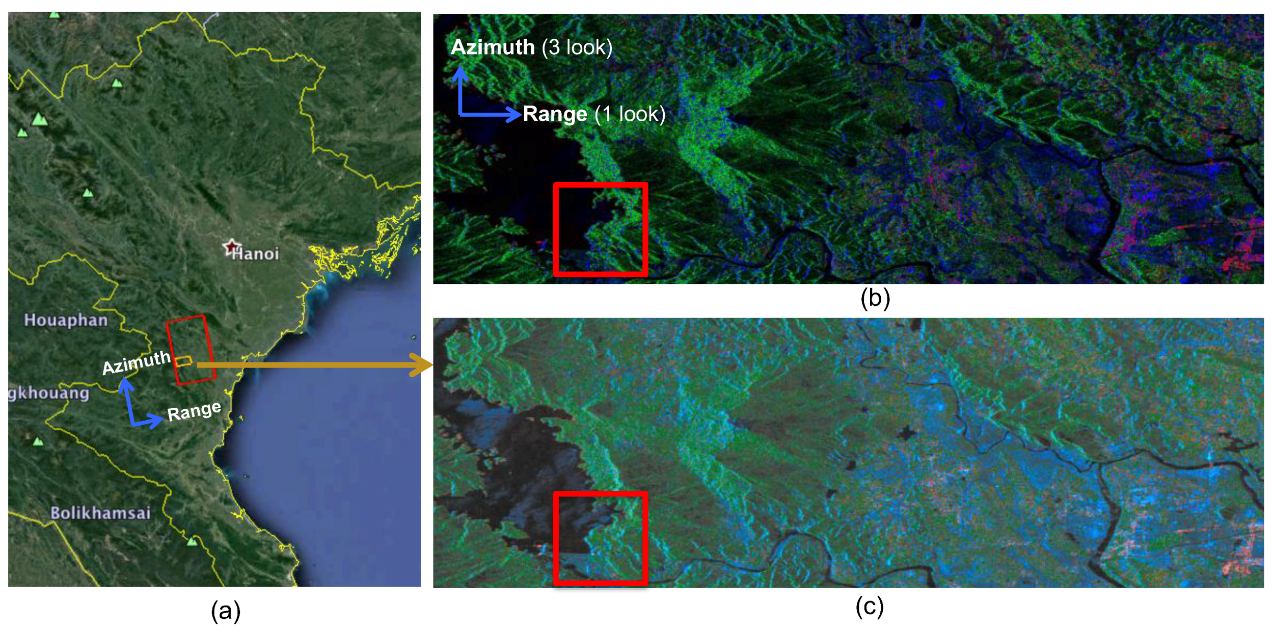
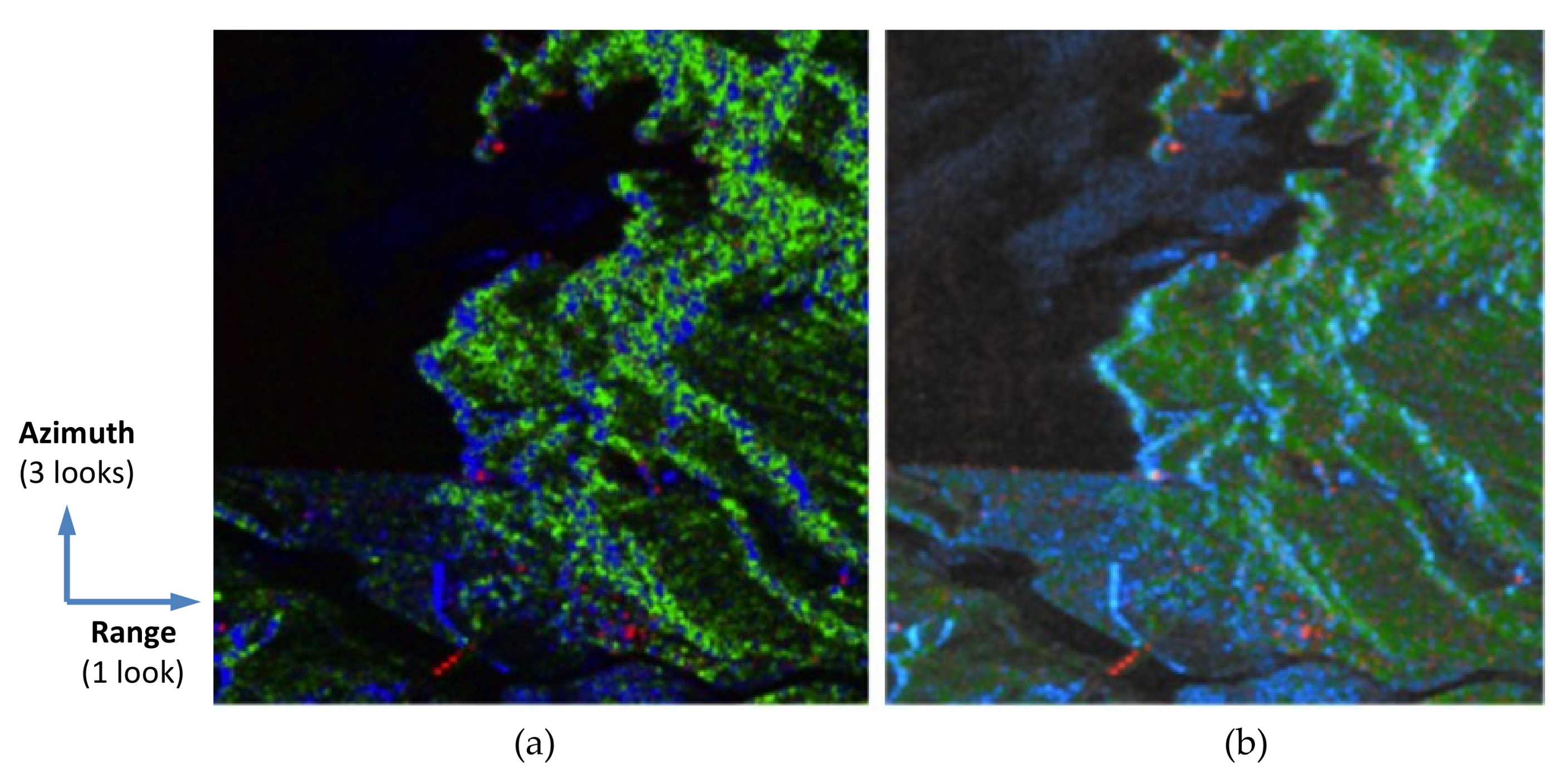
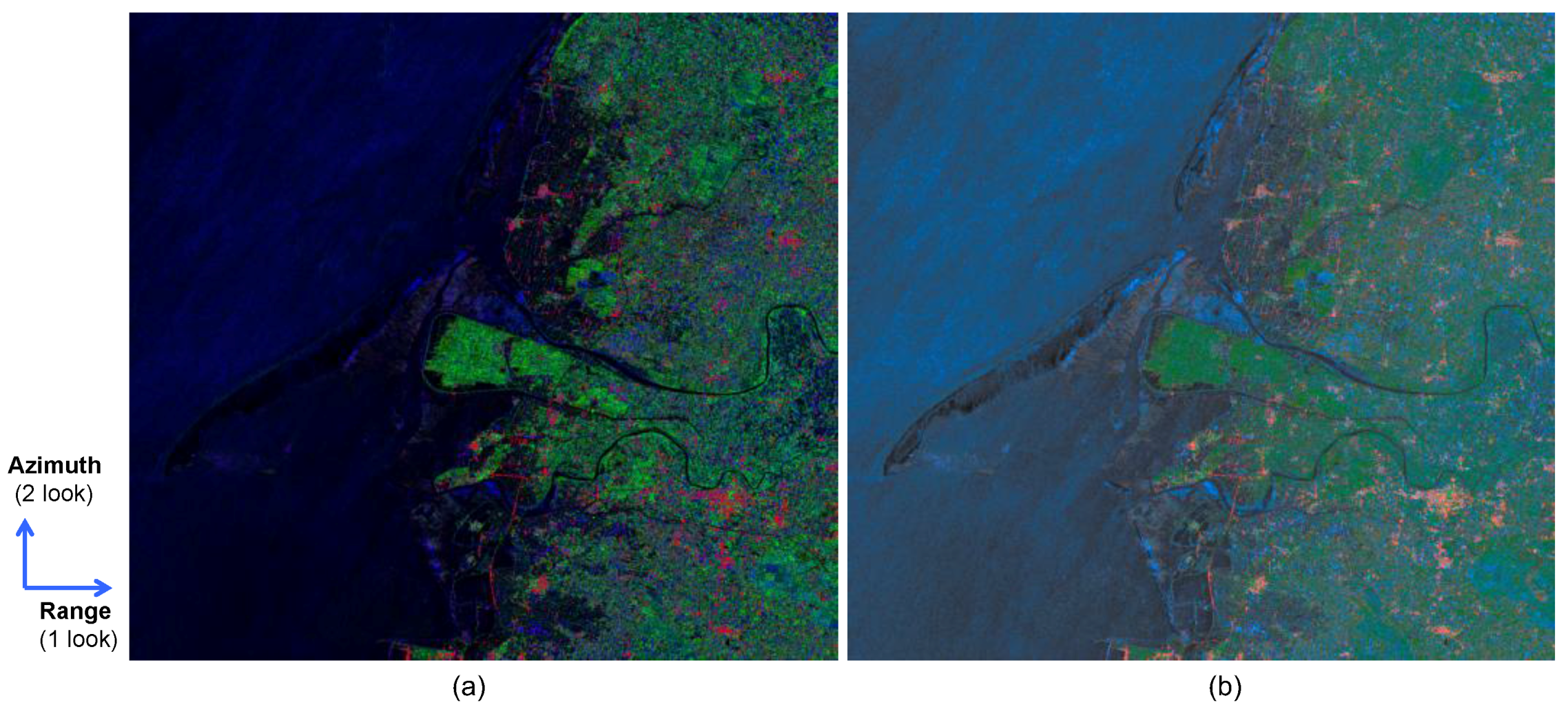
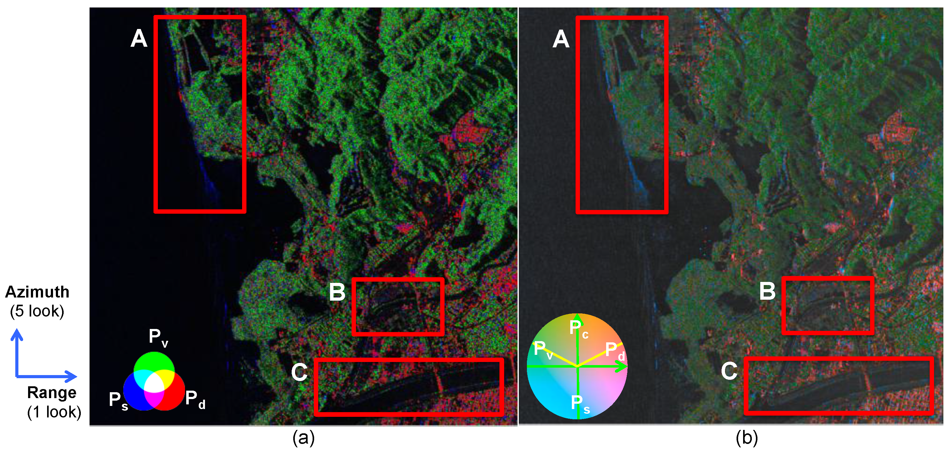
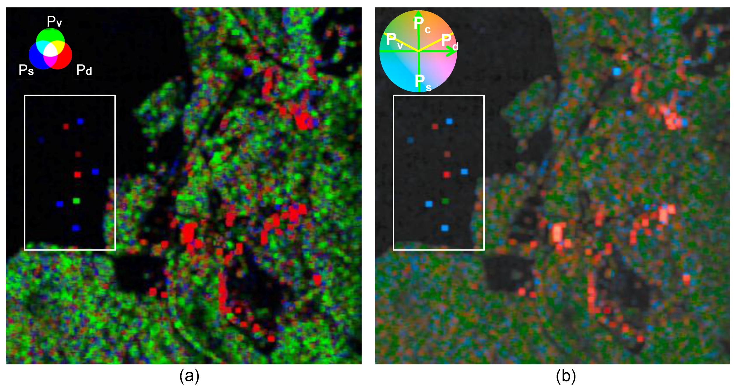
4.3. Application Examples

In Figure 13, we perform color enhancement for an ALOS2 dataset acquired in northern Vietnam with ascending mode in November 2014. The area of interest, as shown in Figure 13b,c, is located to the northwest of Tho Xuan Airport. The red box in Figure 13a indicates a full scene area, within which the orange small box is the region of interest that is shown in the red box in Figure 13b,c with CIE-RGB and CIE-Lab color compositions, respectively. The mountain around the lake in the dam region, covered by the vegetation canopy shown in green, is basically volume scattering dominant. In CIE-RGB color space, these green tones are quite uniform. However, in CIE-Lab color space, variations in the green tone can be seen; in particular, the brighter tone stood out along the ridges, revealing stronger scattering effects. A similar effect is presented on the waterfront near the dam. In this region, it shows mixed blue and green colors that stand for the mixture of surface and volume scattering in less densely vegetated land. To better reveal the difference between the two color enhancement schemes, the enlarged red box in Figure 13 is displayed in Figure 14. The coastline of the lake can be recognized more clearly in CIE-Lab than in CIE-RGB color space because the CIE-RGB color space only includes the four scattering components but excludes the effect of total power.

As another example, we tested the C-band Radarsat-2 data. The strip of sandbank that is in the near range in the left of the image in Figure 15 is much darker because the sandbank is smoother than the rough ocean surface. The sandbank, in CIE-Lab color space, is clearly brought out without destroying other scattering features in ocean and land. To further prove the discernible capability of low returns using CIE-Lab color encoding, we selected A and B regions representing the sandbank and ocean surface, respectively, as shown in Figure 16. The scatter plots of DN values between red, green, and blue in CIE-RGB and CIE-Lab color space are shown in Figure 17. The color contrasts in CIE-Lab space are much higher than those in CIE-RGB space, as is evident from these scatter plots.

At this point, it is worth mentioning that the use of advanced color-coding techniques for the visual exploitation of PolSAR imagery and corresponding time series has already been addressed. In [21], the unsupervised coastline extraction by correlation between co- and cross-polarization data was reported. For coastline segmentation [22], the diffusion-based method was introduced to improve the conventional extraction method. To further demonstrate the use of CIE-Lab, we apply the Spectra Angle Mapper (SAM) [23] calculated from the two class centers given in

Table 1. Comparison of SAM between CIE-RGB and CIE-Lab.

Type	CIE-RGB	CIE-Lab
Green-Red	29.17	16.72
Green-Blue	3.57	8.04
Red-Green-Blue	7.8	18.25

, where the first and second rows show the two channels in 2D, and the last row shows 3D. It is seen that some unreasonable values occur on the Green-Red recorded in CIE-RGB. This is because the Green-Red scatters in CIE-RGB almost mixed together. On the contrary, the overall SAM value in CIE-Lab composition is better than the CIE-RGB compared to the Green-Blue and Red-Green-Blue scatter results. To exploit the potential of the proposed scheme, it is worth applying the scheme to land use/cover classifications from PolSAR imagery [24,25].

As a last example, we used L-band PiSAR data [26] acquired over a calibration site with various corner reflectors deployed at Tottori Dune, Japan on 4 October 2000. Figure 18 shows a comparison of color encoding using CIE-RGB and CIE-Lab for three-component and four-component decomposition. Similar observations from previous examples can also be drawn from Figure 18. The inclusion of total scattering and helix scattering components in the CIE-Lab color space substantially improves the differentiation of details of land cover within the scale class, e.g., vegetation canopy. We selected three regions: A indicates the coast region, and B and C the river bank regions. Near the intersection of water and land, the boundary is much clearer in CIE-Lab because of the inclusion of total power channel. Although the silt deposition in the river bank behaves like smooth surface scatter, supposed to be low in backscattering return, its contrast is enhanced by the total power. The boundary between water and land can be more easily detected by visual inspection. For example, in Region A, the sand bank was obscured by the sea area in the CIE-RGB results because of the dark blue color almost pure specular mechanism with high return power. Because the total power effect is imbedded in CIE-Lab results, the coastline can be extracted more cleanly. In Regions B and C, the many years of sediment on the river bank with low vegetation are evident in the CIE-Lab space. The river can be distinguished from the low-contrast regions in B and C with tinny enhancement that avoids the saturation in other regions.

To further exploit the enhancement power of CIE-Lab color encoding, we analyze the scattering from the array of corner reflectors installed at the calibration site [26], indicated by the white boxes in Figure 19. We see from Figure 19a that several corner reflectors tend to be purely, and thus falsely, in blue, and one reflector was in pure green, indicating volume scattering, which certainly is not correct. This, of course, is caused by color distortion. This distortion is nicely corrected, to a greater extent, in CIE-Lab color space (Figure 19b), where no pure surface and volume scattering falsely appears in corner reflectors, which is indeed double bounce dominant.

5. Conclusions

In this study, we proposed a color-enhancement scheme for fully polarimetric data based on a perceptually uniform CIE-Lab color space. In particular, Yamaguchi’s four-component decomposition with rotation (Y4R) was adopted for target decomposition. It is advantageous to perform color encoding in CIE-Lab color space so that the four scattering components can be displayed simultaneously to enrich the target information content for visualization. The total power is naturally embedded into the encoding, enabling it to enhance target details. From extensive experimental tests on multi-platform, multi-frequency datasets, targets in the same scattering component but with different total power returns can be easily differentiated. It is concluded that the proposed CIE-Lab color encoding is powerful to preserve and enhance the contrast for the same category but different intensity targets. It discerns subtle but vital variations between the two scattering components and thus is suitable for color-encoding the PolSAR data. However, the selection of M and N values affects the visual effect for some special but rare applications such as enhancing extremely strong targets. For this, some modifications are necessary. Another drawback is as a display device system. The CIE-Lab color space must be converted to the RGB color space and hence degrades the visualization effect. To this end, future work shall include more experiments on different decompositions to come up with a generalization scheme in line with using CIE-Lab color-coding.

References

1. Lillesand, T.; Kiefer, R.W.; Chipman, J. Remote Sensing and Image Interpretation, 6th ed.; Wiley: New York, NY, USA, 2007. [Google Scholar]
2. Jensen, J.R. Introductory Digital Image Processing: A Remote Sensing Perspective, 3rd ed.; Prentice Hall: New York, NY, USA, 2004. [Google Scholar]
3. Robertson, P.K.; Robertson, J.F. The application of perceptual color spaces to the display of remotely sensed imagery. IEEE Trans. Geosci. Remote Sens. 1998, 26, 49–59. [Google Scholar] [CrossRef]
4. Amitrano, D.; Martino, G.; Iodice, A.; Riccio, D.; Ruello, G. A New Framework for SAR Multitemporal Data RGB Representation: Rationale and Products. IEEE Trans. Geosci. Remote Sens. 2015, 53, 117–133. [Google Scholar] [CrossRef]
5. Amitrano, D.; Belfiore, V.; Cecinati, F.; Martino, G.; Iodice, A.; Mathieu, P.P.; Medagli, S.; Poreh, D.; Riccio, D.; Ruello, G. Urban Areas Enhancement in Multitemporal SAR RGB Images Using Adaptive Coherence Window and Texture Information. IEEE J. Sel. Top. Appl. Earth Obs. Remote Sens. 2016, 9, 3740–3752. [Google Scholar] [CrossRef]
6. Kartikeyan, B.; Sarkar, A.; Majumder, K.L. A segmentation approach to classification of remote sensing imagery. Int. J. Remote Sens. 1998, 19, 1695–1709. [Google Scholar] [CrossRef]
7. Tyo, J.S.; Pugh, E.N., Jr.; Engheta, N. Colorimetric representations for use with polarization-difference imaging of objects in scattering media. J. Opt. Soc. Am. A 1998, 15, 367–374. [Google Scholar] [CrossRef]
8. Aïnouz, S.; Zallat, J.; Martino, A.D.; Collet, C. Physical interpretation of polarization-encoded images by color preview. Opt. Express 2006, 14, 5916–5927. [Google Scholar] [CrossRef] [PubMed]
9. Freeman, A.; Durden, S.L. A three component scattering model for polarimetric SAR data. IEEE Trans. Geosci. Remote Sens. 1998, 36, 963–973. [Google Scholar] [CrossRef]
10. Lee, J.S.; Pottier, E. Polarimetric Radar Imaging: From Basics to Applications; CRC Press: Baton Rouge, LO, USA, 2009. [Google Scholar]
11. Cloude, S.R. Polarisation: Applications in Remote Sensing; Oxford University Press: Oxford, UK, 2009. [Google Scholar]
12. Yamaguchi, Y.; Moriyama, T.; Ishido, M.; Yamada, H. Four-component scattering model for polarimetric SAR image decomposition. IEEE Trans. Geosci. Remote Sens. 2005, 43, 1699–1706. [Google Scholar] [CrossRef]
13. Yamaguchi, Y.; Sato, A.; Boerner, W.M.; Sato, R.; Yamada, H. Four-component scattering power decomposition with rotation of coherency matrix. IEEE Trans. Geosci. Remote Sens. 2011, 49, 2251–2258. [Google Scholar] [CrossRef]
14. Hunt, R.W.G.; Pointer, M.R. Measuring Colour, 4th ed.; Wiley: New York, NY, USA, 2011. [Google Scholar]
15. Berns, R.S.; Billmeyer, F.W.; Saltzman, M. Billmeyer and Saltzman’s Principles of Color Technology, 3rd ed.; Wiley: New York, NY, USA, 2000. [Google Scholar]
16. Gonzalez, R.C.; Woods, R.E. Digital Image Processing, 2nd ed.; Prentice Hall: Upper Saddle River, NJ, USA, 2002. [Google Scholar]
17. MacAdam, D.L. Visual sensitivities to color differences in daylight. J. Opt. Soc. Am. 1942, 60, 247–274. [Google Scholar] [CrossRef]
18. Sato, A.; Yamaguchi, Y.; Singh, G.; Park, S.E. Four-component scattering power decomposition with extended volume scattering model. IEEE Geosci. Remote Sens. Lett. 2012, 9, 166–170. [Google Scholar] [CrossRef]
19. Cui, Y.; Yamaguchi, Y.; Yang, J.; Park, S.E.; Kobayashi, H.; Singh, G. Three-component power decomposition for polarimetric SAR data based on adaptive volume scatter modeling. Remote Sens. 2012, 4, 1559–1572. [Google Scholar] [CrossRef]
20. Lee, J.S.; Ainsworth, T.L.; Wang, Y. Generalized Polarimetric Model-Based Decompositions Using Incoherent Scattering Models. IEEE Trans. Geosci. Remote Sens. 2013, 52, 2474–2491. [Google Scholar] [CrossRef]
21. Nunziata, F.; Buono, A.; Migliaccio, M.; Benassai, G. Dual-polarimetric C- and X-band SAR data for coastline extraction. IEEE J. Sel. Top. Appl. Earth Obs. Remote Sens. 2016, 9, 4921–4928. [Google Scholar] [CrossRef]
22. Yu, Y.; Acton, S.T. Automated delineation of coastline from polarimetric SAR imagery. Int. J. Remote Sens. 2010, 25, 3423–3438. [Google Scholar] [CrossRef]
23. Yuhas, R.H.; Goetz, A.F.H.; Boardman, J.W. Discrimination among Semi-Arid Landscape Endmembers Using the Spectral Angle Mapper (SAM), 1992, 1, 147–149. Available online: https://ntrs.nasa.gov/search.jsp?R=19940012238 (accessed on 6 March 2017).
24. Buono, A.; Nunziata, F.; Migliaccio, M.; Yang, X.; Li, X. Classification of the Yellow River delta area using fully polarimetric SAR measurements. Int. J. Remote Sens. 2017, 38, 6714–6734. [Google Scholar] [CrossRef]
25. Ferrentino, E.; Nunziata, F.; Migliaccio, M. Full-polarimetric SAR measurements for coastline extraction and coastal area classification. Int. J. Remote Sens. 2017, 38, 7405–7421. [Google Scholar] [CrossRef]
26. Makoto, S.; Seiho, U.; Toshihiko, U.; Hideo, M.; Akitsugu, N.; Tatsuharu, K.; Takeshi, M.; Takeshi, M.; Harunobu, M. Flight Experiments of Airborne High-Resolution Multi-Parameter Imaging Radar, Pi-SAR. J. Commun. Res. Lab. 2000, 49, 127–141. [Google Scholar]
Figure 1. CIE 1964 xy chromaticity diagram.
Remotesensing 10 00545 g001
Figure 2. Resemble of Poincare Sphere ((left), from [8]) and generic CIE-Lab Color Sphere (right).
Remotesensing 10 00545 g002
Figure 3. Mapping function from original digital number (DN) y to enhanced DN x.
Remotesensing 10 00545 g003
Figure 4. Schematic plot of the four scattering components in CIE-Lab color mapping with a different dynamic range for each component (not to scale).
Remotesensing 10 00545 g004
Figure 5. Realignment of the four scattering components on a color wheel of CIE-Lab color space, to enhance the weaker but vital scattering component: (a) all alignments; (b) PsPc alignment.
Remotesensing 10 00545 g005
Figure 6. The profile extracted from upper-right circle. The color are from pistachio to vermilion, black line (a), and the symmetrical color along the a-axis, red line (b) and b-axis, blue line (c).
Remotesensing 10 00545 g006
Figure 7. Flowchart of the proposed color assignment and enhancement for CIE-Lab color space.
Remotesensing 10 00545 g007
Figure 8. The visual effects of changing the 2N% value at the L-axis.
Remotesensing 10 00545 g008
Figure 9. The visual effects of changing the M% value in the ab-plane boundary for N = 1.
Remotesensing 10 00545 g009
Figure 10. CIE-RGB color composition for three linear polarized channels, Pauli vector, and three decomposed components of Y4R. Also shown is the comparison of data slicing (with 5%) effect on the visualization effects: local slicing (left); global slicing (right).
Remotesensing 10 00545 g010
Figure 11. Color Composition using CIE-RGB (left) with 5% local data slicing in total power and CIE-Lab (right) with L-axis N = 1 and ab-plane M = 15 slicing in total power.
Remotesensing 10 00545 g011
Figure 12. CIE-Lab color encodings: (a) Pv alignment with vanished Pc component; (b) Ps alignment with vanished Pc component; (c) PsPc alignment.
Remotesensing 10 00545 g012
Figure 13. Dam region in northern Vietnam (a) Worldview of region of image; (b) CIE-RGB encoded color; (c) CIE-Lab encoded color.
Remotesensing 10 00545 g013
Figure 14. Enlarged dam region: (a) CIE-RGB encoded color; (b) CIE-Lab encoded color.
Remotesensing 10 00545 g014
Figure 15. Radarsat-2 SAR image of a coastal region of western Taiwan: (a) CIE-RGB-encoded color; (b) CIE-Lab-encoded color.
Remotesensing 10 00545 g015
Figure 16. Sandbar region: (a) CIE-RGB-encoded color; (b) CIE-Lab-encoded color.
Remotesensing 10 00545 g016
Figure 17. Scatter plot for Region A (ocean) in blue and Region B (sandbank) in red from Figure 16.
Remotesensing 10 00545 g017
Figure 18. PISAR-encoded color data for Taiwan: (a) CIE-RGB-encoded color with 15% global data slicing; (b) CIE-Lab-encoded color with N = 1 and M = 15.
Remotesensing 10 00545 g018
Figure 19. Comparison of (a) CIE-RGB and (b) CIE-Lab color enhancement for an array of corner reflectors indicated in the inscribed white boxes.
Remotesensing 10 00545 g019