On the Use of Unmanned Aerial Systems for Environmental Monitoring

Abstract

Environmental monitoring plays a central role in diagnosing climate and management impacts on natural and agricultural systems; enhancing the understanding of hydrological processes; optimizing the allocation and distribution of water resources; and assessing, forecasting, and even preventing natural disasters. Nowadays, most monitoring and data collection systems are based upon a combination of ground-based measurements, manned airborne sensors, and satellite observations. These data are utilized in describing both small- and large-scale processes, but have spatiotemporal constraints inherent to each respective collection system. Bridging the unique spatial and temporal divides that limit current monitoring platforms is key to improving our understanding of environmental systems. In this context, Unmanned Aerial Systems (UAS) have considerable potential to radically improve environmental monitoring. UAS-mounted sensors offer an extraordinary opportunity to bridge the existing gap between field observations and traditional air- and space-borne remote sensing, by providing high spatial detail over relatively large areas in a cost-effective way and an entirely new capacity for enhanced temporal retrieval. As well as showcasing recent advances in the field, there is also a need to identify and understand the potential limitations of UAS technology. For these platforms to reach their monitoring potential, a wide spectrum of unresolved issues and application-specific challenges require focused community attention. Indeed, to leverage the full potential of UAS-based approaches, sensing technologies, measurement protocols, postprocessing techniques, retrieval algorithms, and evaluation techniques need to be harmonized. The aim of this paper is to provide an overview of the existing research and applications of UAS in natural and agricultural ecosystem monitoring in order to identify future directions, applications, developments, and challenges.

1. Introduction

Despite the recent and rapid increase in the number and range of Earth observing satellites [1,2,3], the temporal resolution and availability of current very high spatial resolution satellite sensors (less than 10 m) are generally not sufficient nor flexible enough for many quantitative remote sensing applications, and they are thus of limited use in detecting and monitoring the dynamics of surficial environmental processes. Recent advances in Earth observation (i.e., EO) are opening new opportunities for environmental monitoring at finer scales [4]. For instance, CubeSat platforms represent a promising satellite technology, operating predominantly in the visible to near-infrared portion of the electromagnetic spectrum, and provide high spatial and temporal resolution [5]. Nevertheless, most of these satellites are operated by commercial organizations; hence, if short revisit times are required (i.e., for high-frequency monitoring), the cost of image acquisition can become a limiting factor. While manned airborne platforms can, in principle, provide both high spatial resolution and rapid revisit times, in practice, their use is routinely limited by operational complexity, safety, logistics, and cost. Their use becomes feasible only over medium-sized areas and remains largely within the domain of commercial operators. Recent advances in Unmanned Aerial Systems (UAS) technology have created an alternative monitoring platform that provides an opportunity to capture the spatial, spectral, and temporal requirements across a range of applications with relatively small investment. They offer high versatility, adaptability, and flexibility compared with manned airborne systems or satellites, and have the potential to be rapidly and repeatedly deployed for high spatial and temporal resolution data [6].

While UAS systems cannot compete with satellite imagery in terms of spatial coverage, they provide unprecedented spatial and temporal resolutions unmatched by satellite alternatives. Furthermore, they do so at a fraction of the satellite acquisition cost if the area of interest has relatively small extent. For example, a newly tasked high-resolution natural color image (50 cm/pixel) from a satellite (e.g., GeoEye-1) can cost up to 3000 USD. On the other hand, the initial outlay to acquire a single UAS with a natural color camera can be less than 1000 USD (see Appendix A), with this delivering a dataset of high spatial resolution (several cm/pixel). Of course, the additional benefit of the UAS platform is that the temporal resolution is limited only by the number of flights (and power supply/battery capacity), so any cost equivalence is quickly overcome due to repeatability. The costs for acquiring UAS imagery are usually derived from the initial investment, the processing software, data storage, and associated (and ongoing) fieldwork expenses. However, after the initial investment, datasets can be delivered more often and at a higher resolution than by any other EO system.

Matese et al. [7] provided an intercomparison of the acquisition and processing costs of three different platforms (UAS, Aircraft, and Satellite). Their cost model parametrization allows the derivation of the relative cost for the different configurations, showing that UAS is the most cost-effective solution for fields of an extent equal to or less than 20 ha. Their quantitative analyses showed that the approximate total cost of a UAS-derived Normalized Difference Vegetation Index (NDVI) map over a 5 ha field is equal to 400 €/ha, while satellite products may cost about 30% more.

A cost–benefit analysis for monitoring and maintaining parks facilities, such as the Deleo Regional Sports Park, identified a clear economical convenience in the use of UAS for an area with an extent of approximately 10 ha [8]. Of course, the theoretical limit for such economic convenience may be affected by several parameters (e.g., type of vehicle, sensors adopted, frequency of flights, and postprocessing) and this may lead to a nonunique result, but there is a general coherence in the literature that tends to identify such a limit in a lower bound between 10 and 20 ha. Over larger areas, acquisition, georeferencing, and orthorectification costs impact negatively on the economic costs of UAS-derived images.

Of course, it is not an equivalent assessment to compare these platforms on an image-by-image basis, as it is the spatiotemporal richness of the UAS systems that makes their application so transformative. Beyond allowing the high spatial and temporal resolutions needed for many applications, UAS-mounted sensors have several additional advantages which are key across a range of applications. First, they provide rapid access to environmental data, offering the near real-time capabilities required in many applications. The most mature of these is the capacity to share orthomosaic and elevation data, using both commercial and open-source alternatives [9]. Second, UAS satisfy safety requirements and accessibility issues for inspection of otherwise inaccessible sites or for hazard detection and monitoring [10]. Third, the great advantage of UAS is their capacity to collect data in cloudy or hazy conditions that would otherwise obscure satellite retrieval. Analysis of meteorological data has shown that, even with daily revisits of Earth observation satellites, the probability of operating a monitoring service based on optical satellite imagery in rainy regions is about 20%, while the probability of obtaining a usable image with UAS is between 45 and 70% [11]. Perhaps most importantly, operations with UAS are not limited to specific hours (as with sun-synchronous satellite sensors), and, thus, UAS can be used for continuous environmental monitoring.

These aforementioned capabilities, together with the increasing variety and affordability of both UAS and sensor technologies, have stimulated an explosion of interest from researchers across numerous domains [12,13,14,15,16]. Among others, Singh and Frazier [17] provided a detailed meta-analysis on published articles highlighting the diversity of UAS processing procedures, clearly identifying the critical need for a harmonization and standardization among the many possible strategies to acquire and preprocess data to derive UAS-based products.

The dynamic nature and spatial variability of environmental processes that occur at very fine scales require data of an equivalent high spatial and temporal resolution. For successful and efficient monitoring, timely data are necessary, and high flexibility makes the UAS imagery ideal for the task. Specific timing and frequent acquisition of data at very fine scales also enables targeted monitoring of rapid (interannual) changes of environmental features, including plant phenology and growth, extreme events, and hydrological processes. For these reasons, environmental studies were among the first civil applications of the technology in 1990s. Thanks to the significant cost reduction of both vehicles and sensors, and recent developments in data processing software, UAS applications have expanded rapidly in the last decade, stimulating a number of additional and complementary topics spanning full automation of single or multiple vehicles, tracking and flight control systems, hardware and software innovations, tracking of moving targets, and image correction and mapping performance assessment. The growing interest in those applications is reflected in the number of UAS-based research papers published over the last 27 years, with a focus on those being directed towards environmental monitoring (based on a search of the ISI (Internation Scientific Indexing)-web of knowledge using the keywords “UAS” or “UAV”, and “environment”). In particular, the number of applications has seen a particularly prominent increase over the last five years (Figure 1).

In addition to the increasing availability of UAS, recent advances in sensor technologies and analytical capabilities are rapidly expanding the number of potential UAS applications. Increasing miniaturization allows multispectral, hyperspectral, and thermal imaging, as well as Synthetic Aperture Radar (SAR) and LiDAR (Light Detection and Ranging) sensing to be conducted from UAS. As examples of recent UAS-based environmental monitoring applications, work has focused on (a) land cover mapping [18,19]; (b) vegetation state, phenology, and health [20,21]; (c) precision farming/agriculture [22,23,24]; (d) monitoring crop growth, and invasive species infestation [25,26]; (e) atmospheric observations [27]; (f) disaster mapping [28]; (g) soil erosion [29,30]; (h) mapping soil surface characteristics [31,32]; and (i) change detection [33].

Given the research and technological advances in recent years and the rapidly evolving landscape with respect to UAS applications, the aim of this paper is to review the current state of the art in the field of UAS applications for environmental monitoring, with a particular focus on hydrological variables, such as vegetation conditions, soil properties and moisture, overland flow, and streamflow. This review provides a common shared knowledge framework that can be used to guide and address the future activities of the international research network. We divide our review into three sections that focus on different (but related) aspects of UAS-based environmental monitoring: (1) data collection and processing; (2) monitoring natural and agricultural ecosystems; and (3) monitoring river systems. We conclude by summarizing current and emerging issues, potential roadblocks, and other challenges in further advancing the application of UAS in environmental monitoring.

2. Data Collection, Processing, and Limitations

While offering an unprecedented platform to advance spatiotemporal insights across the Earth and environmental sciences, UAS are not without their own operational, processing, and retrieval problems. These range from image blur due to the forward motion of the platform [34], resolution impacts due to variable flying height, orthorectification issues and geometric distortion associated with inadequate image overlap [35], and the spectral effects induced by variable illumination during flight. These and other factors can all affect the subsequent quality of any orthorectified image and, subsequently, the derived products. These are well described in a recent review paper by Whitehead and Hugenholtz [13]. As such, it is essential to consider best practice in the context of (a) mission and flight planning; (b) preflight camera/sensor configuration; (c) in-flight data collection; (d) ground control/ radiometric calibration and correction; (e) geometric and atmospheric corrections; (f) orthorectification and image mosaicking; and (g) extracting relevant products/metrics for remote sensing application. Items (a) and (b) are preflight tasks, (c) and (d) are conducted in the field at the time of survey, and (e)–(g) are postsurvey tasks. Together, these aspects are crucial to data acquisition and postprocessing, which deliver the necessary starting point for subsequent application-specific analysis. However, despite the existence of well-established workflows in photogrammetry, manned aircraft, and satellite-based remote sensing to address such fundamental aspects, UAS systems introduce various additional complexities, which to date have not been thoroughly addressed. Consequently, best practice workflows for producing high-quality remote sensing products from UAS are still lacking, and further studies that focus on validating UAS-collected measurements with robust processing methods are important for improving the final quality of the processed data [36,37].

2.1. Preflight Planning

Flight or mission planning is the first essential step for UAS data acquisition and has a profound impact on the data acquired and the processing workflow. Similar to other remote sensing approaches, a host of parameters must be considered before the actual flight, such as platform specifications, the extent of the study site (area-of-interest), ground sampling distance, payload characteristics, topography of the study site, goals of the study, meteorological forecasts, and local flight regulations. UAS have additional aspects that require further consideration, including the skill level of the pilot, platform characteristics, and actual environmental flight conditions—all of which affect the data characteristics and subsequent phases of processing.

Due to the proliferation of low-cost, off-the-shelf digital cameras, photogrammetry has been the primary implementation of UAS. James and Robson [38] highlighted how unresolved elements of the camera model (lens distortion) can propagate as errors in UAS-DEMs (derived digital elevation models), and how this can be addressed by incorporating oblique images. Other studies have highlighted the importance of flight line configurations [39], as well as minimizing image blur [34]. There is a need to consolidate this evidence to develop best practice guidance for optimizing UAS SfM (structure-from-motion) measurement quality, whilst maintaining ease of use and accessibility.

Accurate absolute orientation (georeferencing) is an important element for UAS surveys, and is fundamental for any multitemporal monitoring or comparison to other datasets. This task is often referred to as registration, and is conventionally dependent on establishing ground control points (GCPs) which are fixed by a higher-order control method (usually Global Navigation Satellite System—GNSS or Global Positioning System). A number of studies have examined the effect of GCP networks (number and distribution) in UAS surveys, showing that significant errors are expected in SfM-based products where GCPs are not adopted [39,40]. Nevertheless, systematic DEM error can be significantly reduced by including properly defined GCPs [41] or incorporating oblique images in the absence of GCP [38].

Best practice can also be drawn from manned aerial photogrammetry. Direct georeferencing is standard practice in aerial photogrammetry, where the position and orientation of the platform are precisely determined using on-board survey-grade differential GNSS and inertial measurement unit (IMU) data combined through an inertial navigation system (INS) [42]. This allows the camera station (exposure) position and orientation to be derived directly, thus eliminating or minimizing the need for ground control points. Therefore, as discussed by Colomina and Molina [35], there is an increasing drive towards achieving centimeter-level direct georeferencing for UAS using alternative GNSS/IMU configurations, precise point positioning (PPP), and dual-frequency GNSS.

2.2. Sensors

The large availability of UAS equipped with visible (VIS) commercial cameras (see

Table A1. Optical cameras available for UAS and their main characteristics (* Abbreviations: APS = Advanced Photo System type-C; FF = Full Frame; MILC = Mirrorless Interchangeable-Lens Camera; SF = Small Frame).

Manufacturer and Model	Sensor Type Resolution (MPx)	FormatType *	Sensor Size (mm2)	Pixel Pitch (μm)	Weight (kg)	Frame Rate (fps)	Max Shutter Speed (s−1)	Approx. Price ($)
Canon EOS 5DS	CMOS 51	FF	36.0 × 24.0	4.1	0.930	5.0	8000	3400
Sony Alpha 7R II	CMOS 42	FF MILC	35.9 × 24.0	4.5	0.625	5.0	8000	3200
Pentax 645D	CCD 40	FF	44.0 × 33.0	6.1	1.480	1.1	4000	3400
Nikon D750	CMOS 24	FF	35.9 × 24.0	6.0	0.750	6.5	4000	2000
Nikon D7200	CMOS 24	SF	23.5 × 15.6	3.9	0.675	6.0	8000	1100
Sony Alpha a6300	CMOS 24	SF MILC	23.5 × 15.6	3.9	0.404	11.0	4000	1000
Pentax K-3 II	CMOS 24	SF	23.5 × 15.6	3.9	0.800	8.3	8000	800
Foxtech Map-01	CMOS 24	APS-C	23.5 × 15.6	3.9	0.155	6	4000	880
Canon EOS 7D Mark II	CMOS 20	SF	22.3 × 14.9	4.1	0.910	10.0	8000	1500
Panasonic Lumix DMC GX8	CMOS 20	SF MILC	17.3 × 13.0	3.3	0.487	10.0	8000	1000
Sony QX1	CMOS 20	APS-C	23.2 × 15.4	4.3	0.216	3.5	4000	500
Ricoh GXR A16	CMOS 16	SF	23.6 × 15.7	4.8	0.550	2.5	3200	650

) has been the main driver for research that has explored the potential use of low-cost sensors for vegetation monitoring [43,44,45,46]. Among the many available visible spectral indices, the Normalized Green–Red Difference Index (NGRDI) and Excessive Green (ExG) indices have been used to provide acceptable or high levels of accuracy in vegetation mapping studies. Such vegetation indices may be a cost-effective tool for plant biomass estimation and establishing yield variation maps for site-specific agricultural decision-making.

Over the last five to eight years, near-infrared (NIR) multi- and hyperspectral sensors have become more widely available for UAS. Modified off-the-shelf RGB (red–green–blue) cameras—initially very popular [47]—have now started to be replaced by dedicated multispectral or hyperspectral cameras, as these have reduced in cost and weight. For instance, lightweight hyperspectral sensors for UAS are now available from different vendors (e.g., SPECIM; HYSPEX; HeadWall; see Appendix A), offering more defined and discrete spectral responses compared to the modified RGB or multiband cameras. Multispectral cameras commonly employ multiple lenses, which introduce band-to-band offsets that need to be adequately corrected in order to avoid artefacts introduced into the combined multiband product [48,49]. Both multispectral and hyperspectral cameras require radiometric calibration and atmospheric corrections to convert the recorded digital numbers (DN) to surface reflectance values to enable reliable assessment of ground features, comparison of repeated measurements, and reliable determination of spectral indices [50]. Although DN are frequently utilized directly to derive vegetation indices (e.g., NDVI), illumination differences between (and within) surveys mean that the use of these values is generally inappropriate, particularly for quantitative studies.

Radiometric calibration normally involves in-field measurement of reference natural or artificial targets with a field spectroradiometer [50,51,52] and calibration of individual cameras requiring significant additional effort. Some current multispectral cameras (e.g., Parrot Sequoia, MicaSense RedEdge—see

Table A2. Multispectral cameras available on the market for UAS and their main characteristics (* selectable bands).

Manufacturer and Model	Resolution (Mpx)	Size (mm)	Pixel Size (μm)	Weight (kg)	Number of Spectral Bands	Spectral Range (nm)	Approx. Price ($)
Tetracam MCAW6 (Global shutter)	1.3	-	4.8 × 4.8	0.55	6	450–1000 (*)	16,995
Tetracam MCAW12 (Global shutter)	1.3	-	4.8 × 4.8	0.6	12	450–1000 (*)	34,000
Tetracam MicroMCA4 Snap (Global shutter)	1.3	115.6 × 80.3 × 68.1	4.8 × 4.8	0.497	4	450–1000 (*)	9995
Tetracam MicroMCA6 Snap (Global shutter)	1.3	115.6 × 80.3 × 68.1	4.8 × 4.8	0.53	6	450–1000 (*)	14,995
Tetracam MicroMCA12 Snap (Global shutter)	1.3	115.6 × 155 × 68.1	4.8 × 4.8	1	12	450–1000 (*)	29,995
Tetracam MicroMCA6 RS (Rolling shutter)	1.3	115.6 × 80.3 × 68.1	4.8 × 4.8	0.53	6	450–1000 (*)	12,995
Tetracam MicroMCA12 RS (Rolling shutter)	1.3	115.6 × 155 × 68.1	4.8 × 4.8	1	12	450–1000 (*)	25,995
Tetracam ADC micro	3.2	75 × 59 × 33	3.2 × 3.2	0.9	6	520–920 (Equiv. to Landsat TM2, 3, 4)	2995
Quest Innovations Condor-5 ICX 285	7	150 × 130 × 177	6.45 × 6.45	1.4	5	400–1000	-
Parrot Sequoia	1.2	59 × 41 × 28	3.75 × 3.75	0.72	4	550–810	5300
MicaSense RedEdge		120 × 66 × 46		0.18	5	475–840	4900
Sentera Quad	1.2	76 × 62 × 48	3.75 × 3.75	0.170	4	400–825	8500
Sentera High Precision NDVI and NDRE	1.2	25.4 × 33.8 × 37.3	3.75 × 3.75	0.030	2	525–890	-
Sentera Multispectral Double 4K	12.3	59 × 41 × 44.5	-	0.080	5	386–860	5000
SLANTRANGE 3P NDVI	3	146 × 69 × 57	-	0.350	4	410–950	4500
Mappir Survey2	16	59 × 41 × 30	1.34 × 1.34	0.047	1–6 (filters)—one lens	395–945	280
Mappir Survey3	12	59 × 41.5 × 36	1.55 × 1.55	0.050	1–4 (filters)—one lens	395–945	400
Mappir Kernel	14.4	34 × 34 × 40	1.4 × 1.4	0.045	19+ (filters)—six array lens	395–945	1299

) include a downwelling irradiance sensor and calibrated reflectance panel in order to address some of the requirements of radiometric calibration. This is beneficial, but it does not address the full complexity of radiometric calibration, and artefacts will remain. Other aspects, such as bidirectional reflectance (modelled through the bidirectional reflectance distribution function (BRDF)) and image vignetting, introduce further uncertainties for image classification. While the most appropriate workflow for dealing with multispectral imagery depends to some extent on the complexity of the subsequent application (e.g., basic vegetation indices or reflectance-based image classification), the growing body of literature and recent sensor improvements support the development of best practice guidelines for the environmental UAS community.

Hyperspectral sensors (

Table A3. Hyperspectral cameras suitable for UAS and their main characteristics.

Manufacturer and Model	Lens	Size (mm2)	Pixel Size (μm)	Weight (kg)	Spectral Range (nm)	Spectral Bands (N) (Resolution, nm)	Peak SNR	Approx. Price ($)
Rikola Ltd. hyperspectral camera	CMOS	5.6 × 5.6	5.5	0.6	500–900	40 (10 nm)	-	40,000
Headwall Photonics Micro-hyperspec X-series NIR	InGaAs	9.6 × 9.6	30	1.025	900–1700	62 (12.9 nm)	-	-
BaySpec’s OCI-UAV-1000	C-mount	10 × 10 × 10	N/A	0.272	600–1000	100 (5 nm)/20–12 (15 nm)	-	-
HySpex Mjolnir V-1240	-	25 × 17.5 × 17	0.27 mrad	4.0	400–1000	200 (3 nm)	>180	-
HySpex Mjolnir S-620	-	25.4 × 17.5 × 17	0.54 mrad	4.5	970–2500	300 (5.1 nm)	>900	-
Specim-AISA KESTREL16	push-broom	99 × 215 × 240		2.3	600–1640	Up to 350 (3–8 nm)	400–600	-
Cornirg microHSI 410 SHARK	CCD/CMOS	136 × 87 × 70.35	11.7 μm	0.68	400–1000	300 (2 nm)	-	-
Resonon Pika L		10.0 × 12.5 × 5.3	5.86	0.6	400–1000	281 (2.1 nm)	368–520	-
CUBERT (S185)	Snapshot + PAN	19 × 42 × 65		0.49	450–995	125 (8 mm)	-	50,000

) can be briefly mentioned as extensions of the discussion surrounding multispectral sensors and related considerations of radiometric calibration and atmospheric correction. Over the last five years, there has been increasing interest in hyperspectral imaging sensors [9,53]. While these are still more expensive than multispectral systems, they offer significant potential for quantitative soil vegetation and crop studies. UAS hyperspectral imagers typically offer contiguous narrow bands in the VIS-–NIR (near-infrared) portion of the spectrum. Existing cameras include pushbroom and, more recently, frame capture technology. Depending on the capture mechanism, there are typically artefacts related to noninstantaneous (time delay) capture across bands, or physical offsets between bands [53]. There has also been interest in (nonimaging) UAS-mounted (hyperspectral) spectrometers [54].

In the hyperspectral domains, high radiometric accuracy and accurate reflectance retrieval are key factors to further exploit this technology [55]. Accordingly, practices from the manned platforms bearing hyperspectral sensors can be adopted in UAS applications, such as the new super-vicarious calibration method suggested by Brook and Ben-Dor [51,56]. This study used artificial targets to assess data quality, to correct at-sensor radiance, and to generate a high-quality reflectance data-cube. Technologies that have been introduced also include light sensors in the SWIR (shortwave infrared) region, with these produced specifically for UAS applications (HeadWall).

UAS broadband thermal imaging sensors (see

Table A4. Representative thermal cameras suitable for UAS and their main characteristics.

Manufacturer and Model	Resolution (Px)	Sensor Size (mm2)	Pixel Pitch (μm)	Weight (kg)	Spectral Range (μm)	Thermal Sensitivity (mK)	Approx. Price ($)
FLIR Duo Pro 640	640 × 512	10.8 × 8.7	17	<0.115	7.5–13.5	50	10,500
FLIR Duo Pro 336	336 × 256	5.7 × 4.4	17	<0.115	7.5–13.5	50	7500
FLIR Duo R	160 × 120	-	-	0.084	7.5–13.5	50	2200
FLIR Tau2 640	640 × 512	N/A	17	<0.112	7.5–13.5	50	9000
FLIR Tau2 336	336 × 256	N/A	17	<0.112	7.5–13.5	50	4000
Optris PI 450	382 × 288	-	-	0.320	7.5–13	130	7000
Optris PI 640	640 × 480	-	-	0.320	7.5–13	130	9700
Thermoteknix Miricle 307 K	640 × 480	16.0 × 12.0	25	<0.170	8.0–12.0	50	-
Thermoteknix Miricle 110 K	384 × 288	9.6 × 7.2	25	<0.170	8.0–12.0	50/70	-
Workswell WIRIS 640	640 × 512	16.0 × 12.8	25	<0.400	7.5–13.5	30/50	-
Workswell WIRIS 336	336 × 256	8.4 × 6.4	25	<0.400	7.5–13.5	30/50	-
YUNCGOETEU	160 × 120	81 × 108 × 138	12	0.278	8.0–14.0	<50	-

) measure the emitted radiance of the Earth’s surface (from which the brightness temperature can be calculated) typically between 7.5 and 13.5 μm. Key considerations relate to spatial resolution and thermal sensitivity, with the latter now achieving 40–50 mK. Thermal UAS remote sensing also requires consideration of radiometric calibration and accounting for vignetting and other systematic effects, as discussed by Smigaj et al. [57]. With the aim to provide a description of the potential of a thermal camera mounted on a UAS, an example of a thermal image providing the surface temperature (in degrees Celsius) obtained over a vineyard of Aglianico is given in Figure 2. This information can be used to compute the vegetation state or soil water content given the strong relationship existing between these variables and the surface energy balance. Here, one can appreciate the high level of detail offered by this technology in the description of a patchy area of vegetation.

LiDAR sensors (see

Table A5. Laser scanners suitable for UAS and their main characteristics.

Manufacturer and Model	Scanning Pattern	Range (m)	Weight (kg)	Angular Res. (deg)	FOV (deg)	Laser Class and λ (nm)	Frequency (kp/s)	Aprox. Price ($)
ibeo Automotive Systems IBEO LUX	4 Scanning parallel lines	200	1	(H) 0.125 (V) 0.8	(H) 110 (V) 3.2	Class A 905	22	-
Velodyne HDL-32E	32 Laser/detector pairs	100	2	(H)–(V) 1.33	(H) 360 (V) 41	Class A 905	700	-
RIEGL VQ-820-GU	1 Scanning line	>1000	25.5	(H) 0.01 (V) N/A	(H) 60 (V) N/A	Class 3B 532	200	-
Hokuyo UTM-30LX-EW	1080 distances in a plane	30	0.37	(H) 0.25 (V) N/A	(H) 270 (V) N/A	Class 1905	200	-
Velodyne Puck Hi-Res	Dual Returns	100	0.590	(H)–(V) 0.1–0.4	(H) 360 (V) 20	Class A-903	-	-
RIEGL VUX-1UAV	Parallel scan lines	150	3.5	0.001°	330	Class A-NIR	200	>120,000
Routescene—UAV LidarPod	32 Laser/detector pairs	100	1.3	(H)–(V) 1.33	(H) 360 (V) 41	Class A-905	-	-
Quanergy M8-1	8 laser/detector pairs	150	0.9	0.03–0.2°	(H) 360 (V) 20	Class A-905	-	-
Phoenix Scout	Dual Returns	120	1.65	-	(H) 360 (V) 15	Class 1-905	300	>66,000
Phoenix ALS-32	32 Laser/detector pairs	120	2.4	-	(H) 360 (V) 10–30	Class 1-905	700	>120,500
YellowScan Surveyor	Dual returns	100	1.6	0.125	360	Class 1-905	300	>93,000
YellowScan Vx	Parallel scan lines	100	2.5–3	-	360	Class 1-905	100	>93,000

) are also becoming more commonplace on UAS platforms, as increasingly lightweight systems become achievable (although <3 kg maximum take-off weight is still challenging). There is particular interest in UAS LiDAR for forestry applications, especially in relation to classifying and quantifying structural parameters (e.g., forest height, crown dimensions; [58]).

Each of the sensors listed in this or the previous section allows one to derive information with some sort of drawback. For instance, hyperspectral and thermal cameras can provide a more appropriate description of the physiological state of vegetation, but at the expense of the spatial resolution, costs, and complexity of processing and calibration. Using LiDAR technology provides detailed information about the vegetation structure but is demanding in terms of the data processing and costs of the sensor. Therefore, there is a critical need to identify a standard approach for specific tasks that can reduce sensor errors and associated elaboration, enhancing the reliability of UAS observations.

A review of the available cameras and sensors for UAS applications is provided in the Appendix in order to guide future studies and activities in this field. Tables include a number of pieces of technical information along with an approximate price quote when available.

2.3. Software

Alongside sensor technological developments, low-cost (and particularly open source) software has been vital in enabling the growth in UAS for environmental and other applications. UAS-based photogrammetry can produce products of a similar accuracy to those achievable through manned airborne systems [35]. This has been underpinned by the development of SfM software, which offers a user-friendly and low-cost alternative to conventional digital photogrammetric processing. This includes proprietary structure-from-motion (SfM) software such as Agisoft Photoscan and Pix4D, which is significantly more affordable than most conventional photogrammetric software. Moreover, there has also been development of open source SfM software, including VisualSfM, Bundler, Apero-MicMac, OpenDroneMap, etc. Nevertheless, although different and efficient software solutions are available, the computational cost of the elaboration is critical and it can require several days of data processing. Cloud-based platforms such as DroneDeploy or DroneMapper offer the possibility to integrate and share aerial data, but also to derive orthomosaics with light processing workloads. While this has made photogrammetry more accessible to nonexperts, quantification of uncertainty remains an ongoing challenge [59]. This is because SfM relaxes some of the conventional expectations in terms of image block geometry and data acquisition.

3. Monitoring Agricultural and Natural Ecosystems

Natural and agricultural ecosystems are influenced by climatic forcing, physical characteristics, and management practices that are highly variable in both time and space. Moreover, vegetation state changes can often occur within a short period of time [60,61] due to unfavorable growing conditions or climatic extremes (e.g., heat waves, heavy storms, etc.). Therefore, in order to capture such features, monitoring systems need to provide accurate information over large areas with a high revisit frequency [62]. UAS platforms provide one such technology that is enabling new horizons in vegetation monitoring. For instance, the high resolution of UAS imagery has led to a significant increase in the overall accuracy in species-level vegetation classification, monitoring vegetation status, weed infestations, estimating biomass, predicting yields, detecting crop water stress and/senescent leaves, reviewing herbicide applications, and pest control.

3.1. Vegetation Monitoring and Precision Agriculture

Precision agriculture [63] has been the most common environmental monitoring application of UAS. High-spatial-resolution UAS imagery enables much earlier and more cost-effective detection, diagnosis, and corrective action of agricultural management problems compared to low-resolution satellite imagery. Therefore, UAS may provide the required information to address the needs of farmers or other users at the field scale, enabling them to make better management decisions with minimal costs and environmental impact [64,65,66].

Vegetation state can be evaluated and quantified through different vegetation indices from images acquired in the visible, red edge, and near-infrared spectral bands. Depending on their formulation, these can display a strong correlation with soil coverage and Leaf and Green Area Index (LAI and GAI), Crop Nitrogen Uptake (QN), chlorophyll content, water stress detection, canopy structure, photosynthesis, yield, and/or growing conditions [67,68,69]. As such, these vegetation indices may be exploited to monitor biophysical parameters.

Among the many available vegetation indices, the Normalized Difference Vegetation Index (NDVI) is one that is most widely used [70,71,72]. UAS-NDVI maps can be at least comparable to those obtained from satellite visible observations and become highly relevant for a timely assessment of crop health status, with capacity to provide immediate feedback to the farmer. NDVI surveys performed with UAS, aircraft, and satellite demonstrate that low-resolution images generally fail in representing intrafield variability and patterns in fields characterized by small vegetation gradients and high vegetation patchiness [7]. Moreover, UAS-derived NDVIs have shown better agreement with ground-based NDVI observations compared to satellite-derived NDVIs in several crop and natural vegetation types [73,74,75]. As an example of the achievable resolution that can be obtained from UAVs, relative to some available high-resolution commercial satellite sensors, Figure 3 shows a multi-sensor sequence of imagery collected over a date palm plantation in Saudi Arabia. The observed differences between vegetation patterns and resolvable resolution observed by UAS (compared to available satellite platforms) are clearly identified. The relative advantages of UAS in providing a level of detail that is comparable to field observations (or in deriving NDVI or other related vegetation indices for more in depth assessment) is illustrated by its capability of capturing both within and between canopy behavior.

In the last decade, particular attention has been given to the monitoring of vineyards because of their high economic value. Johnson et al. [76] proposed one of the first applications where different sensors were used for determining measures related to chlorophyll function and photosynthetic activity, LAI, and plant health status (among other variables) to mapping vigor differences within fields. More recently, Zarco-Tejada et al. [52,77,78,79,80] demonstrated the potential for monitoring specific variables such as crop water stress index, photosynthetic activity, and carotenoid content in vineyards using multispectral, hyperspectral, and thermal cameras.

Based upon author experiences, farmers have expressed particular interest in monitoring crop conditions for the quantification of water demand, nitrogen status, or infestation treatments. Several of the variables or indices described above may be used for rapid detection of crop pest outbreaks or for mapping the status of crops. Likewise, monitoring soil water content is critical for determining efficient irrigation scheduling. The topsoil moisture content can be derived using RGB, NIR, and thermal bands [81]. The effective amount of water stored in the subsurface can be obtained by exploiting mathematical relationships between surface measurements and the root zone soil moisture, such as the Soil Moisture Analytical Relationship (SMAR) [82,83].

As a further example, Sullivan et al. [84] observed that the thermal infrared (TIR) emittance was highly sensitive to canopy state and can be used for monitoring soil water content, stomatal conductance, and canopy cover. TIR has similarly been used for the monitoring and estimation of soil surface characteristics such as microrelief and rill morphology [85], soil water repellency [86], soil surface macropores [87], skin surface soil permeability [88], and overland and rill flow velocities by using thermal tracers [89,90].

More specifically, the TIR emittance displays a negative correlation with stomatal conductance and canopy closure, indicating increasing canopy stress as stomatal conductance and canopy closure decreased. The crop water stress index (CWSI) [91,92] calculated from leaf water potential can be used to determine the required frequency, timing, and duration of watering. In this regard, the CWSI, derived with a UAS equipped with a thermal camera, is frequently adopted to quantify the physiological status of plants, and, more specifically, leaf water potential in experimental vineyards or orchards [52,80,93,94,95,96]. The derived CWSI maps can serve as important inputs for precision irrigation. Time series of thermal images can also be used to determine the variation in water status [97].

Using VIS–NIR (400–1000 nm) hyperspectral and multispectral analyses of simulated data has shown that soil attributes can be extracted from these spectral regions, particularly those most commonly used by the current UAS platforms [98,99,100]. These studies demonstrated that the VIS-NIR spectral region alone can open up new frontiers in soil mapping (as well as soil moisture content retrieval) using on-board multi- and hyperspectral UAS sensors without using heavyweight sensors operating in the SWIR (1–2.5 μm) region. Aldana-Jague et al. [32] mapped soil surface organic carbon content (<0.5 cm) at 12 cm resolution exploiting six bands between 450 and 1050 nm acquired by low-altitude multispectral imagers. D’Oleire-Oltmanns et al. [30] showed the applicability of UAS for measuring, mapping, and monitoring soil erosion at 5 cm resolution with an accuracy between 0.90 and 2.7 cm in the horizontal and 0.70 cm in the vertical directions. Detailed information about soil erosion can enhance proper soil management at the plot scale [31].

Such tools were further explored by Zhu et al. [22], who investigated the ability to quantify the differences in soil nitrogen application rates using digital images taken from a UAS compared with ground-based hyperspectral reflectance and chlorophyll content data. They suggested that aerial photography from a UAS has the potential to provide input in support of crop decision-making processes, minimizing field sampling efforts, saving both time and money, and enabling accurate assessment of different nitrogen application rates. Therefore, such information may serve as input to other agricultural systems, such as tractors or specific UAS, that optimize fertilizer management.

UAS can also improve agronomical practices. Costa et al. [101] described an architecture that can be employed to implement a control loop for agricultural applications where UAS are responsible for spraying chemicals on crops. Application of chemicals is controlled by the feedback obtained from a wireless sensor network (WSN) deployed on the crop field. They evaluated an algorithm to adjust the UAS route under changes in wind (intensity and direction) to minimize the waste of pesticides. Peña et al. [102,103] explored the optimization of herbicide applications in weed–crop systems using a series of UAS multispectral images. The authors computed multiple data, which permitted both calculation of herbicide requirements and estimation of the overall cost of weed management operations in advance. They showed that the ability to discriminate weeds was significantly affected by the imagery spectra (type of camera) used as well as the spatial (flight altitude) and temporal (the date of the study) resolutions.

Among these technical advantages and constraints, the importance of the limitation of operational rules in using UAS in several countries needs to be highlighted. As an example, Jeunnette and Hart [24] developed a parametric numerical model to compare aerial platform options (UAS vs airborne) to support agriculture in developing countries characterized by highly fragmented fields, but manned systems are still more competitive from an operational and cost/efficiency point of view because of the present limitations in altitude, distance, and speed of UAS. In particular, UAS become cost-competitive when they are allowed to fly higher than 300 m AGL (above ground level), while current limits are set around 120–150 m. This is a critical limitation for the use of UAS along with the fact that flights should be within visible line of sight (VLOS) in many jurisdictions.

All the applications described highlight the potential use of UAS in developing advanced tools for precision agriculture applications and for vegetation monitoring in general. With time, both technological advances and legislation will evolve and likely converge, further advancing the efficient use of such technologies.

3.2. Monitoring of Natural Ecosystems

As with agricultural ecosystems, the proliferation of UAS-based remote sensing techniques has opened up new opportunities for monitoring and managing natural ecosystems [12,104,105,106]. In fact, UAS provides options and opportunities to collect data at appropriate spatial and temporal resolutions to describe ecological processes and allow better surveying of natural ecosystems placed in remote, inaccessible, or difficult- and/or dangerous-to-access sites. As examples, some habitats (e.g., peat bogs) can be damaged through on-ground surveys, while UAS positioned several meters above the surface can provide a near-comparable level of information as that obtained through plot-based measurements (e.g., canopy cover by species). UAS are also useful for undertaking rapid surveys of habitats such as mangroves, where access is often difficult and plot-based surveys take far longer to complete (see Figure 4).

UAS therefore offer the potential to overcome these limitations and have been applied to monitor a disparate range of habitats and locations, including tropical forests, riparian forests, dryland ecosystems, boreal forests, and peatlands. Pioneering researchers have been using UAS to monitor attributes such as plant population [107,108]; biodiversity and species richness [109,110]; plant species invasion [111]; restoration ecology [112]; disturbances [113]; phenology [114]; pest infestation in forests [115,116]; and land cover change [117].

Many studies have focused on the retrieval of vegetation structural information to support forest assessment and management [118,119]. For instance, information on the plant and canopy height can be obtained from stereo images [120,121], which can be used to estimate above-ground biomass (see for example Figure 4). 3D maps of canopy can also be used to distinguish between trunks, branches, and foliage [121].

UAS represent a promising option enabling timely, fast, and precise monitoring that is important for many plant species, particularly those that are invasive [122,123,124]. Flexibility of the data acquisition enabled by the UAS is very important, since plants are often more distinct from the surrounding vegetation in certain times of their growing season [125]. Besides rapid monitoring of newly invaded areas, the UAS methodology enables prediction/modelling of invasion spread that can be driven by a combination of factors, such as habitat and species characteristics, human dispersal, and disturbances [126]. Legal constraints limiting the use of UAS to unpopulated areas can be especially problematic for monitoring invasive species that tend to prefer urban areas. Still, the UAS technology can greatly reduce costs of extensive field campaigns and eradication measures [127].

UAS are also revolutionizing the management of quasi-natural ecosystems, such as restored habitats and managed forests. They have been used to quantify spatial gap patterns in forests in order to support the planning of common forest management practices such as thinning [128] or to support restoration monitoring. For example, Quilter et al. [129] used UAS for monitoring streams and riparian restoration projects in inaccessible areas on Chalk Creek (Utah). Knoth et al. [130] applied a UAS-based NIR remote sensing approach to monitor a restored cut-over bog and Ludovisi et al. [21] also used TIR data to determine the response of forest to drought in relation to forest tree breeding programs and genetic improvement.

4. River Systems and Floods

Satellite data are widely used to monitor natural hazards (e.g., floods, earthquakes, volcanic eruptions, wildfire, etc.) at national and international scales [131]. This popularity is due to their wide coverage, spectral resolution, safety, and rate of update [132,133]. Nevertheless, UAS have also been adopted for rapid assessment following natural extreme events and in the context of humanitarian relief and infrastructure assessment [28]. According to Quaritsch et al. [134], UAS should be utilized as a component of a network of sensors for natural disaster management. Although there are a number of technological barriers, which must be overcome before UAS can be utilized in a more automated and coordinated manner, their potential for disaster response is significant [135]. Given the UAS potential, we expect significant advances in the fields of hydrology, geomorphology, and hydraulics, where there is a significant opportunity for the use of UAS for monitoring river systems, overland flows, or even urban floods.

Flow Monitoring

River systems and stream flows can be monitored by remotely integrating the techniques of water body observation, vegetation mapping, DEM generation, and hydrological modelling. Satellite sensors in the visible, infrared, and microwave ranges are currently used to monitor rivers and to delineate flood zones [136,137,138]. These methods are generally used only over large rivers or areas of inundation in order to detect changes at the pixel level. UAS can describe river dynamics, but with a level of detail that is several orders of magnitude greater and can enable distributed flow measurements over any river system and in difficult-to-access environments.

In this context, the integration of UAS imagery and optical velocimetry techniques has enabled full remote kinematic characterization of water bodies and surface flows. Optical techniques, such as Large-Scale Particle Image Velocimetry (LSPIV, [139]) and Particle Tracking Velocimetry (PTV [140]), are efficient yet nonintrusive flow visualization methods that yield a spatially distributed estimation of the surface flow velocity field based on the similarity of image sequences. Proof-of-concept experiments have demonstrated the feasibility of applying LSPIV from manned aerial systems to monitor flood events [141,142]. More recently, videos recorded from a UAS have been analyzed with LSPIV to reconstruct surface flow velocity fields of natural stream reaches [143,144]. This provides a detailed Lagrangian insight into river dynamics that is valuable in calibrating numerical models.

Most of these experimental observations entail a low-cost UAS hovering above the region of interest for a few seconds (the observation time should be adjusted to the flow velocity and camera acquisition frequency). An RGB camera is typically mounted onboard and installed with its optical axis perpendicular to the captured field of view to circumvent orthorectification [145]. To facilitate remote photometric calibration, Tauro et al. [145] adopted a UAS equipped with a system of four lasers that focus points at known distances in the field of view. In several experimental settings, the accuracy of surface flow velocity estimations from UAS was found to be comparable to (or even better than) that of traditional ground-based LSPIV configurations [146]. In fact, compared to fixed implementations, UAS enable capture of larger fields of view with a diffuse rather than direct illumination. Such optical image velocimetry techniques can measure flow velocity fields over extended regions rather than pointwise, and at temporal resolutions comparable to or even better than Acoustic Doppler Velocimetry (ADV) based on the presence of detectable features on the water surface [147].

In this context, UAS technology is expected to considerably aid in flood monitoring and mapping. In fact, flood observation is a considerable challenge for space-borne passive imagery, mostly due to the presence of dense cloud cover, closed vegetation canopies, and the satellite revisit time and viewing angle [133,148]. Although SAR satellite sensors (e.g., Sentinel-1, TerraSAR-X, RADARSAT-2) can overcome these visibility limitations, they are unable to provide the submeter-level spatial resolution necessary for detailed understanding of flood routing and susceptibility. Applying UAS with an appropriate flight mode may overcome some of these issues, allowing for rapid and safe monitoring of inundations and measurement of flood hydrological parameters [149]. This is possible also because most platforms are quite stable in windy conditions (less than 5 m/s in the case of multirotors).

Challenges for the widespread adoption and incorporation of UAS for flow monitoring have commonalities with both agricultural and ecosystems monitoring, including the coupling of measurements from multiple sensors through accurate and efficient processing workflows. Specific to streamflow measurement, these include (i) optimization of SfM workflows to enable extraction of terrestrial and subsurface topographies through accurate image registration using automatic or direct georeferencing techniques; (ii) the determination of water levels through image- (e.g., SfM; [150]), sensor- (e.g., laser, radar; [151]), and turbulence-derived metrics [152]; and (iii) the derivation of flow velocities through appropriate techniques (e.g., PIV/PTV), based on the characteristics of flow, duration of observation, seeding density, etc.). The task of combining these data and developing workflows that are capable of rapidly producing synoptic river flow measurements based on the range of available inputs is an ongoing challenge to ensure UAS-based measurements are able to fully support water resource management and civil protection agencies.

In this context, hyperspectral sensors can also be used to extend the range of water monitoring applications. Potential examples include sediment concentration, chlorophyll distribution, blooming algae status, submerged vegetation mapping, bathymetry, and chemical and organic waste contaminations [153,154].

5. Final Remarks and Challenges

UAS-based remote sensing provides new advanced procedures to monitor key variables, including vegetation status, soil moisture content, and stream flow. A detailed description of such variables will increase our capacity to describe water resource availability and assist agricultural and ecosystem management. Our manuscript provides an overview of some of the recent applications in field-based UAS surficial environmental monitoring. The wide range of applications testifies to the great potential of these techniques, but, at the same time, the variety of methodologies adopted is evidence that there is still need for harmonization efforts. The variety of available platforms, sensors, and specificity of any particular case study have stimulated a proliferation of a huge number of specific algorithms addressing flight planning, image registration, calibration and correction, and derivation of indices or variables. However, there is no evidence of comprehensive comparative studies that enable the user to select the most appropriate procedure for any specific need.

A review of the literature carried out herein allowed the identification of a number of outstanding issues in the use of UAS for environmental monitoring. Among others, we selected the following that require specific attention:

(i)

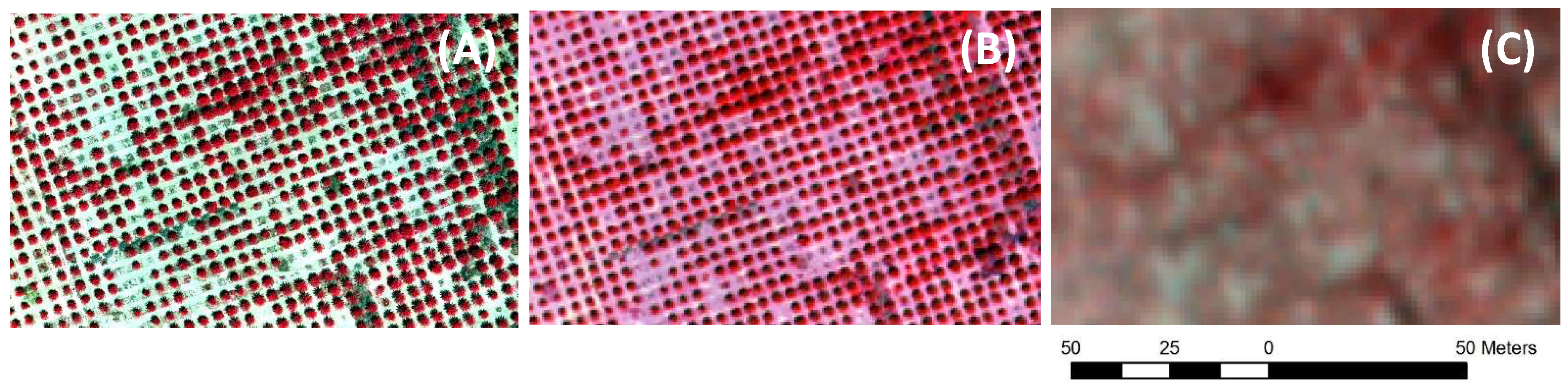
While a direct comparison between different methodologies (UAS, manned airborne, and satellite) is challenging, it was found that UAS systems represent a cost-effective monitoring technique over small regions (<20 ha). For larger extents, manned airborne or satellite platforms may become more effective options, but only when the temporal advantage of the UAS is not considered.

(ii)

The limited extent of the studied areas reduces the relative budget available, increasing the fragmentation of the adopted procedures and methodologies.

(iii)

Government regulations restricting the Ground Sample Distance (GSD) and the UAS flight mode are limiting the economic advantages related to their use and some potential applications, particularly in urban environments.

(iv)

The wide range of experiences described highlighted the huge variability in the strategies, methodologies, and sensors adopted for each specific environmental variable monitored. This identifies the need to find unifying principles in UAS-based studies.

(v)

Vulnerability of UAS to weather conditions (e.g., wind, rain) can alter quality of the surveys.

(vi)

There are also technical limits, such as weather constraints (strong wind and/or rain), high elevations, or high-temperature environments that can be challenging for most of the devices/sensors and respective UAS operators (see, e.g., [155]).

(vii)

The geometric and radiometric limitations of current lightweight sensors make the use of this technology challenging.

(viii)

The high spatial resolution of UAS data generates high demand on data storage and processing capacity.

(ix)

There is a clear need for procedures to characterize and correct the sensor errors that can propagate in the subsequent mosaicking and related data processing.

(x)

Finally, a disadvantage in the use of UAS is represented by the complexity associated to their use that is comparable to that of satellites. In fact, satellite applications are generally associated to a chain of processing assuring the final quality of data. In the case of UAS, all this is left to the final user or researcher, requiring additional steps in order to be able to use the retrieved data.

It should be recognized that the UAS sector has received much less funding to address the existing gaps in technology and processing chains needed to produce useable images than, for instance, satellite-based programs (Figure 5). However, this is one of the reasons why there is much potential for further improvements in the technology and its use. One particular benefit of UAV improvements is related to the potential benefit that could be directed towards satellite-based observations, which can leverage the utilization of highly detailed UAS data. Given the spatiotemporal advantage of UAS systems, they can provide much higher return periods, offering several flights per day to study very dynamic processes at high spatial resolution, such as physiological response of vegetation to heat or even rapid flooding events. The combination of these data allows an advanced satellite test-bed for examining scale effects due to spatial resolution, identifying the most suitable acquisition time, establishing the effects of temporal resolution, incorporating suitable spectral bands, and establishing needed radiometric resolution, etc., all of which provide feedback to developing improved space-borne platforms in a way that ground-based monitoring alone can never replicate. Moreover, the capability to achieve a resolution comparable with the scale of field measurements gives the opportunity to address the issue of within-pixel spatial heterogeneity observed by satellites.

With time, natural selection will likely deliver the most efficient collection and processing solutions for different contexts and applications, but there is still a significant amount of work needed to drive this change. Therefore, a major challenge for the scientific community is to foster this process by providing some guidance in the wide range of possibilities offered by the market. On the other side of this, the private sector of UAS developers are also investing in this field, accelerating the evolution of the technology. Among the many advances, it is interesting to mention the following:

• One of the aspects directly impacting the area that is able to be sensed is the limited flight times of UAS. This problem is currently managed by mission planning that enables management of multiple flights. Technology is also offering new solutions that will extend the flight endurance up to several hours, making the use of UAS more competitive. For instance, new developments in batteries suggest that the relatively short flying time imposed by current capacity will be significantly improved in the future [156]. In this context, another innovation introduced in the most recent vehicles is an integrated energy supply system connected with onboard solar panels that allow flight endurance to be extended from 40–50 min up to 5 h, depending on the platform.
• The relative ground sampling distance affects the quality of the surveys, but is often not compensated for. This limitation can now be solved by implementing 3D flight paths that follow the surface in order to maintain a uniform GSD. Currently, only a few software suites (e.g., UgCS, eMotion 3) use digital terrain models to adjust the height path of the mission in order to maintain consistent GSD.
• The influence of GSD may be reduced by increasing flight height, making UAS even more cost-competitive (by increasing sensed areas), but current legislation in many jurisdictions limits this to between 120 and 150 m and to within visible line of sight (VLOS). In this context, the development of microdrones will significantly reduce risk associated with their use, and relax some of the constraints due to safety requirements.
• Recent and rapid developments in sensor miniaturization, standardization, and cost reduction have opened new possibilities for UAS applications. However, limits remain, especially for commercial readymade platforms that are used the most among the scientific community.
• Sensor calibration remains an issue, especially for hyperspectral sensors. For example, vegetation can be measured in its state and distribution using RGB, multispectral, hyperspectral, and thermal cameras, as well as with LiDAR.
• Image registration, correction, and calibration remain major challenges. The vulnerability of UAS to weather conditions (wind, rain) and the geometric and radiometric limitations of current lightweight sensors have stimulated the development of new algorithms for image mosaicking and correction. In this context, the development of open source and commercial SfM software allows image mosaicking to be addressed, but radiometric correction and calibration is still an open question that may find a potential solution through experience with EO. Moreover, the development of new mapping-quality cameras has already significantly improved spatial registration and will likely help to also improve the overall quality of the UAS imagery.

Technological advances are strongly supporting the diffusion of these technologies over a wide range of fields, including hydrology. On the other hand, the research community must address significant challenges in standardizing the methodologies adopted. All environmental variables (e.g., vegetation, soil moisture, and river flow) can be measured using different sensors and algorithms, but a comprehensive assessment of the performances of each of these methods and procedures is required. Such efforts may help to improve our capacity in describing the spatiotemporal processes at both the field and the river basin scale. Moreover, UAS technology can be easily integrated with other devices and tools (cell phone, fixed installations, etc.), allowing advances in agricultural practices and hydrometeorological monitoring.

Technology and scientific research have a clear path to follow that has already (largely) been traced by manned aerial photogrammetry and Earth observation from satellites. In fact, current observational practices have already addressed several of the problems that UAS-based observations are facing (e.g., image mosaicking, sensor calibration, radiometric calibration, etc.). Nevertheless, the ensemble of such problems connected to the proper use of UAS introduces a data processing complexity that is comparable to or slightly larger than that of satellites (see Figure 5) and makes their use difficult even for an experienced scientist without clear guidance.

There is a growing need to define harmonized approaches able to channel the efforts of all these studies and identify the optimal strategy for UAS-based monitoring. The challenge for the research is to define a clear and referenced workflow starting from the planning and acquisition of the data to the generation and interpretation of maps. In particular, we envisage the need to stimulate a comparative experiment able to assess the reliability of different procedures and a combination of algorithms in order to identify the most appropriate methodology for environmental monitoring in different hydroclimatic conditions. The definition of clear and specific procedures may also help in the definition of new legislation at the European scale, removing some of the actual restrictions that limit the potential use of UAS in a wider range of contexts.

Ultimately, it will be the integration of UAS platforms with different techniques, including traditional instruments, fixed and mobile camera surveys, satellite observations, and geomorphological analyses, that will almost certainly deliver an improved characterization of Earth and environmental systems. Apart from providing improved spatial and temporal coverage, such a strategy of integrated observation will inevitably improve our knowledge of agricultural, hydraulic, geomorphological, ecological, and hydrological dynamics, and provide a basis for advancing our understanding of process description and behavior across space and time scales.

References

1. Belward, A.S.; Skøien, J.O. Who Launched What, When and Why; Trends in Global Land-Cover Observation Capacity from Civilian Earth Observation Satellites. ISPRS J. Photogramm. Remote Sens. 2015, 103, 115–128. [Google Scholar] [CrossRef]
2. Hand, E. Startup Liftoff. Science 2015, 348, 172–177. [Google Scholar] [CrossRef] [PubMed]
3. Wekerle, T.; Bezerra Pessoa Filho, J.; Eduardo Vergueiro Loures da Costa, L.; Gonzaga Trabasso, L. Status and Trends of Smallsats and Their Launch Vehicles—An Up-to-Date Review. J. Aerosp. Technol. Manag. 2017, 9, 269–286. [Google Scholar] [CrossRef]
4. McCabe, M.F.; Rodell, M.; Alsdorf, D.E.; Miralles, D.G.; Uijlenhoet, R.; Wagner, W.; Lucieer, A.; Houborg, R.; Verhoest, N.E.C.; Franz, T.E.; et al. The future of Earth observation in hydrology. Hydrol. Earth Syst. Sci. 2017, 21, 3879–3914. [Google Scholar] [CrossRef]
5. McCabe, M.F.; Aragon, B.; Houborg, R.; Mascaro, J. CubeSats in hydrology: Ultrahigh-resolution insights into vegetation dynamics and terrestrial evaporation. Water Resour. Res. 2017, 53, 10017–10024. [Google Scholar] [CrossRef]
6. Pajares, G. Overview and Current Status of Remote Sensing Applications Based on Unmanned Aerial Vehicles (UAVs). Photogramm. Eng. Remote Sens. 2015, 81, 281–329. [Google Scholar] [CrossRef]
7. Matese, A.; Toscano, P.; Di Gennaro, S.F.; Genesio, L.; Vaccari, F.P.; Primicerio, J.; Belli, C.; Zaldei, A.; Bianconi, R.; Gioli, B. Intercomparison of UAV, Aircraft and Satellite Remote Sensing Platforms for Precision Viticulture. Remote Sens. 2015, 7, 2971–2990. [Google Scholar] [CrossRef]
8. Dustin, M.C. Monitoring Parks with Inexpensive UAVs: Cost Benefits Analysis for Monitoring and Maintaining Parks Facilities. Ph.D. Thesis, University of Southern California, Los Angeles, CA, USA, 2015. [Google Scholar]
9. Lucieer, A.; Jong, S.M.D.; Turner, D. Mapping landslide displacements using Structure from Motion (SfM) and image correlation of multi-temporal UAV photography. Progr. Phys. Geog. 2014, 38, 97–116. [Google Scholar] [CrossRef]
10. Watts, A.C.; Ambrosia, V.G.; Hinkley, E.A. Unmanned aircraft systems in remote sensing and scientific research: Classification and Considerations of use. Remote Sens. 2012, 4, 1671–1692. [Google Scholar] [CrossRef]
11. Van der Wal, T.; Abma, B.; Viguria, A.; Previnaire, E.; Zarco-Tejada, P.J.; Serruys, P.; van Valkengoed, E.; van der Voet, P. Fieldcopter: Unmanned aerial systems for crop monitoring services. Precis. Agric. 2013, 13, 169–175. [Google Scholar]
12. Anderson, K.; Gaston, K.J. Lightweight unmanned aerial vehicles will revolutionize spatial ecology. Front. Ecol. Environ. 2013, 11, 138–146. [Google Scholar] [CrossRef]
13. Whitehead, K.; Hugenholtz, C.H. Remote sensing of the environment with small unmanned aircraft systems (UASs), part 1: A review of progress and challenges. J. Unmanned Veh. Syst. 2014, 2, 69–85. [Google Scholar] [CrossRef]
14. Whitehead, K.; Hugenholtz, C.H.; Myshak, S.; Brown, O.; LeClair, A.; Tamminga, A.; Barchyn, T.E.; Moorman, B.; Eaton, B. Remote sensing of the environment with small unmanned aircraft systems (UASs), part 2: Scientific and commercial applications. J. Unmanned Veh. Syst. 2014, 2, 86–102. [Google Scholar] [CrossRef]
15. Adão, T.; Hruška, J.; Pádua, L.; Bessa, J.; Peres, E.; Morais, R.; Sousa, J.J. Hyperspectral imaging: A review on UAV-based sensors, data processing and applications for agriculture and forestry. Remote Sens. 2017, 9, 1110. [Google Scholar] [CrossRef]
16. Tauro, F.; Selker, J.; van de Giesen, N.; Abrate, T.; Uijlenhoet, R.; Porfiri, M.; Manfreda, S.; Caylor, K.; Moramarco, T.; Benveniste, J.; et al. Measurements and Observations in the XXI century (MOXXI): Innovation and multidisciplinarity to sense the hydrological cycle. Hydrolog. Sci. J. 2018, 63, 169–196. [Google Scholar] [CrossRef]
17. Singh, K.K.; Frazier, A.E. A meta-analysis and review of unmanned aircraft system (UAS) imagery for terrestrial applications. Int. J. Remote Sens. 2018, 1–21. [Google Scholar] [CrossRef]
18. Bryson, M.; Reid, A.; Ramos, F.; Sukkarieh, S. Airborne Vision-Based Mapping and Classification of Large Farmland Environments. J. Field Robot. 2010, 27, 632–655. [Google Scholar] [CrossRef]
19. Akar, O. Mapping land use with using Rotation Forest algorithm from UAV images. Eur. J. Remote Sens. 2017, 50, 269–279. [Google Scholar] [CrossRef]
20. Bueren, S.K.; Burkart, A.; Hueni, A.; Rascher, U.; Tuohy, M.P.; Yule, I.J. Deploying four optical UAV-based sensors over grassland: Challenges and limitations. Biogeosciences 2015, 12, 163–175. [Google Scholar] [CrossRef] [Green Version]
21. Ludovisi, R.; Tauro, F.; Salvati, R.; Khoury, S.; Mugnozza Scarascia, G.; Harfouche, A. UAV-based thermal imaging for high-throughput field phenotyping of black poplar response to drought. Front. Plant Sci. 2017, 8, 1681. [Google Scholar] [CrossRef] [PubMed]
22. Zhu, J.; Wang, K.; Deng, J.; Harmon, T. Quantifying Nitrogen Status of Rice Using Low Altitude UAV-Mounted System and Object-Oriented Segmentation Methodology. In Proceedings of the ASME International Design Engineering Technical Conferences and Computers and Information in Engineering Conference, San Diego, CA, USA, 30 August–2 September 2009; pp. 1–7. [Google Scholar]
23. Urbahs, A.; Jonaite, I. Features of the use of unmanned aerial vehicles for agriculture applications. Aviation 2013, 17, 170–175. [Google Scholar] [CrossRef]
24. Jeunnette, M.N.; Hart, D.P. Remote sensing for developing world agriculture: Opportunities and areas for technical development. In Proceedings of the Remote Sensing for Agriculture, Ecosystems, and Hydrology XVIII, Edinburgh, UK, 26–29 September 2016. [Google Scholar]
25. Samseemoung, G.; Soni, P.; Jayasuriya, H.P.W.; Salokhe, V.M. An Application of low altitude remote sensing (LARS) platform for monitoring crop growth and weed infestation in a soybean plantation. Precis. Agric. 2012, 13, 611–627. [Google Scholar] [CrossRef]
26. Alvarez-Taboada, F.; Paredes, C.; Julián-Pelaz, J. Mapping of the Invasive Species Hakea sericea Using Unmanned Aerial Vehicle (UAV) and WorldView-2 Imagery and an Object-Oriented Approach. Remote Sens. 2017, 9, 913. [Google Scholar] [CrossRef]
27. Witte, B.M.; Singler, R.F.; Bailey, S.C.C. Development of an Unmanned Aerial Vehicle for the Measurement of Turbulence in the Atmospheric Boundary Layer. Atmosphere 2017, 8, 195. [Google Scholar] [CrossRef]
28. Stone, H.; D’Ayala, D.; Wilkinson, S. The Use of Emerging Technology in Post-Disaster Reconnaissance Missions; EEFIT Report; Institution of Structural Engineers: London, UK, 2017; 25p. [Google Scholar]
29. Frankenberger, J.R.; Huang, C.; Nouwakpo, K. Low-altitude digital photogrammetry technique to assess ephemeral gully erosion. In Proceedings of the IEEE International Geoscience and Remote Sensing Symposium (IGARSS 2008), Boston, MA, USA, 7–11 July 2008; pp. 117–120. [Google Scholar]
30. d’Oleire-Oltmanns, S.; Marzolff, I.; Peter, K.D.; Ries, J.B. Unmanned aerial vehicle (UAV) for monitoring soil erosion in Morocco. Remote Sens. 2012, 4, 3390–3416. [Google Scholar] [CrossRef]
31. Quiquerez, A.; Chevigny, E.; Allemand, P.; Curmi, P.; Petit, C.; Grandjean, P. Assessing the impact of soil surface characteristics on vineyard erosion from very high spatial resolution aerial images (Côte de Beaune, Burgundy, France). Catena 2014, 116, 163–172. [Google Scholar] [CrossRef]
32. Aldana-Jague, E.; Heckrath, G.; Macdonald, A.; van Wesemael, B.; Van Oost, K. UAS-based soil carbon mapping using VIS-NIR (480-1000 nm) multi-spectral imaging: Potential and limitations. Geoderma 2016, 275, 55–66. [Google Scholar] [CrossRef]
33. Niethammer, U.; James, M.R.; Rothmund, S.; Travelletti, J.; Joswig, M. UAV-based remote sensing of the Super Sauze landslide: Evaluation and results. Eng. Geol. 2012, 128, 2–11. [Google Scholar] [CrossRef]
34. Sieberth, T.; Wackrow, R.; Chandler, J.H. Automatic detection of blurred images in UAV image sets. ISPRS J. Photogramm. Remote Sens. 2016, 122, 1–16. [Google Scholar] [CrossRef]
35. Colomina, I.; Molina, P. Unmanned aerial systems for photogrammetry and remote sensing: A review. ISPRS J. Photogramm. Remote Sens. 2014, 92, 79–97. [Google Scholar] [CrossRef]
36. Mesas-Carrascosa, F.J.; Rumbao, I.C.; Berrocal, J.A.B.; Porras, A.G.F. Positional quality assessment of orthophotos obtained from sensors on board multi-rotor UAV platforms. Sensors 2014, 14, 22394–22407. [Google Scholar] [CrossRef] [PubMed]
37. Ai, M.; Hu, Q.; Li, J.; Wang, M.; Yuan, H.; Wang, S. A robust photogrammetric processing method of low-altitude UAV images. Remote Sens. 2015, 7, 2302–2333. [Google Scholar] [CrossRef]
38. James, M.R.; Robson, S. Mitigating systematic error in topographic models derived from UAV and ground-based image networks. Earth Surf. Process. Landf. 2014, 39, 1413–1420. [Google Scholar] [CrossRef]
39. Peppa, M.; Mills, J.P.; Moore, P.; Miller, P.E.; Chambers, J.C. Accuracy assessment of a UAV-based landslide monitoring system. Int. Arch. Photogramm. Remote Sens. Spat. Inf. Sci. 2016, 41, 895–902. [Google Scholar] [CrossRef]
40. Eltner, A.; Schneider, D. Analysis of Different Methods for 3D Reconstruction of Natural Surfaces from Parallel-Axes UAV Images. Photogramm. Record 2015, 30, 279–299. [Google Scholar] [CrossRef]
41. James, M.R.; Robson, S.; d’Oleire-Oltmanns, S.; Niethammer, U. Optimising UAV topographic surveys processed with structure-from-motion: Ground control quality, quantity and bundle adjustment. Geomorphology 2017, 280, 51–66. [Google Scholar] [CrossRef]
42. Toth, C.; Jóźków, G. Remote sensing platforms and sensors: A survey. ISPRS J. Photogramm. Remote Sens. 2016, 115, 22–36. [Google Scholar] [CrossRef]
43. Geipel, J.; Link, J.; Claupein, W. Combined spectral and spatial modeling of corn yield based on aerial images and crop surface models acquired with an unmanned aircraft system. Remote Sens. 2014, 6, 10335–10355. [Google Scholar] [CrossRef]
44. Torres-Sanchez, J.; Pena, J.M.; de Castro, A.I.; Lopez-Granados, F. Multi-temporal mapping of the vegetation fraction in early-season wheat fields using images from UAV. Comput. Electron. Agric. 2014, 103, 104–113. [Google Scholar] [CrossRef]
45. Saberioon, M.M.; Amina, M.S.M.; Anuar, A.R.; Gholizadeh, A.; Wayayokd, A.; Khairunniza-Bejo, S. Assessment of rice leaf chlorophyll content using visible bands at different growth stages at both the leaf and canopy scale. Int. J. Appl. Earth Obs. Geoinform. 2014, 32, 35–45. [Google Scholar] [CrossRef]
46. Jannoura, R.; Brinkmann, K.; Uteau, D.; Bruns, C.; Joergensen, R.G. Monitoring of crop biomass using true colour aerial photographs taken from a remote controlled hexacopter. Biosyst. Eng. 2015, 129, 341–351. [Google Scholar] [CrossRef]
47. Hunt, E.R.; Hivel, W.D.; Fujikawa, S.J.; Linden, D.S.; Daughtry, C.S.T.; McCarty, G.W. Acquisition of NIR-green-blue digital photographs from unmanned aircraft for crop monitoring. Remote Sens. 2010, 2, 290–305. [Google Scholar] [CrossRef]
48. Laliberte, A.S.; Goforth, M.A.; Steele, C.M.; Rango, A. Multispectral Remote Sensing from Unmanned Aircraft: Image Processing Workflows and Applications for Rangeland Environments. Remote Sens. 2011, 3, 2529–2551. [Google Scholar] [CrossRef]
49. Jhan, J.-P.; Rau, J.-Y.; Haala, N.; Cramer, M. Investigation of parallax issues for multi-lens multispectral camera band co-registration. Int. Arch. Photogramm. Remote Sens. Spat. Inf. Sci. 2017, XLII-2/W6, 157–163. [Google Scholar] [CrossRef]
50. Lu, B.; He, Y. Species classification using Unmanned Aerial Vehicle (UAV)-acquired high spatial resolution imagery in a heterogeneous grassland. ISPRS J. Photogramm. 2017, 128, 73–85. [Google Scholar] [CrossRef]
51. Brook, A.; Ben-Dor, E. Supervised vicarious calibration (SVC) of hyperspectral remote-sensing data. Remote Sens. Environ. 2011, 115, 1543–1555. [Google Scholar] [CrossRef]
52. Zarco-Tejada, P.J.; Gonzalez-Dugo, V.; Berni, J.A.J. Fluorescence, temperature and narrow-band indices acquired from a UAV platform for water stress detection using a microhyperspectral imager and a thermal camera. Remote Sens. Environ. 2012, 117, 322–337. [Google Scholar] [CrossRef]
53. Honkavaara, E.; Rosnell, T.; Oliveira, R.; Tommaselli, A. Band registration of tuneable frame format hyperspectral UAV imagers in complex scenes. ISPRS J. Photogramm. 2017, 134, 96–109. [Google Scholar] [CrossRef]
54. Burkart, A.; Aasen, H.; Alonso, L.; Menz, G.; Bareth, G.; Rascher, U. Angular dependency of hyperspectral measurements over wheat characterized by a novel UAV based goniometer. Remote Sens. 2015, 7, 725–746. [Google Scholar] [CrossRef] [Green Version]
55. Ben-Dor, E.; Chabrillat, S.; Demattê, J.A.M.; Taylor, G.R.; Hill, J.; Whiting, M.L.; Sommer, S. Using imaging spectroscopy to study soil properties. Remote Sens. Environ. 2009, 113, S38–S55. [Google Scholar] [CrossRef]
56. Brook, A.; Ben-Dor, E. Supervised vicarious calibration (SVC) of multi-source hyperspectral remote-sensing data. Remote Sens. 2015, 7, 6196–6223. [Google Scholar] [CrossRef]
57. Smigaj, M.; Gaulton, R.; Suarez, J.C.; Barr, S.L. Use of miniature thermal cameras for detection of physiological stress in conifers. Remote Sens. 2017, 9, 20. [Google Scholar] [CrossRef]
58. Sankey, T.; Donager, J.; McVay, J.; Sankey, J.B. UAV LiDAR and hyperspectral fusion for forest monitoring in the southwestern USA. Remote Sens. Environ. 2017, 195, 30–43. [Google Scholar] [CrossRef]
59. James, M.R.; Robson, S.; Smith, M.W. 3-D uncertainty-based topographic change detection with structure-from-motion photogrammetry: Precision maps for ground controland directly georeferenced surveys. Earth Surf. Process. Landf. 2017, 42, 1769–1788. [Google Scholar] [CrossRef]
60. Manfreda, S.; Caylor, K.K. On the Vulnerability of Water Limited Ecosystems to Climate Change. Water 2013, 5, 819–833. [Google Scholar] [CrossRef]
61. Manfreda, S.; Caylor, K.K.; Good, S. An Ecohydrological framework to explain shifts in vegetation organization across climatological gradients. Ecohydrology 2017, 10, 1–14. [Google Scholar] [CrossRef]
62. Atzberger, C. Advances in remote sensing of agriculture: Context description, existing operational monitoring systems and major information needs. Remote Sens. 2013, 5, 949–981. [Google Scholar] [CrossRef]
63. Zhang, C.; Kovacs, J.M. The application of small unmanned aerial systems for precision agriculture: A review. Precis. Agric. 2012, 13, 693. [Google Scholar] [CrossRef]
64. Huang, Y.; Thomson, S.J.; Hoffmann, W.C.; Lan, Y.; Fritz, B.K. Development and prospect of unmanned aerial vehicle technologies for agricultural production management. Int. J. Agric. Biol. Eng. 2013, 6, 1–10. [Google Scholar]
65. Link, J.; Senner, D.; Claupein, W. Developing and evaluating an aerial sensor platform (ASP) to collect multispectral data for deriving management decisions in precision farming. Comput. Electron. Agric. 2013, 94, 20–28. [Google Scholar] [CrossRef]
66. Zhang, C.; Walters, D.; Kovacs, J.M. Applications of low altitude remote sensing in agriculture upon farmer requests—A case study in northeastern Ontario, Canada. PLoS ONE 2014, 9, e112894. [Google Scholar] [CrossRef] [PubMed]
67. Helman, D.; Givati, A.; Lensky, I.M. Annual evapotranspiration retrieved from satellite vegetation indices for the Eastern Mediterranean at 250 m spatial resolution. Atmos. Chem. Phys. 2015, 15, 12567–12579. [Google Scholar] [CrossRef]
68. Gago, J.; Douthe, C.; Coopman, R.; Gallego, P.; Ribas-Carbo, M.; Flexas, J.; Escalona, J.; Medrano, H. UAVs challenge to assess water stress for sustainable agriculture. Agric. Water Manag. 2015, 153, 9–19. [Google Scholar] [CrossRef]
69. Helman, D.; Lensky, I.M.; Osem, Y.; Rohatyn, S.; Rotenberg, E.; Yakir, D. A biophysical approach using water deficit factor for daily estimations of evapotranspiration and CO2 uptake in Mediterranean environments. Biogeosciences 2017, 14, 3909–3926. [Google Scholar] [CrossRef]
70. Lacaze, B.; Caselles, V.; Coll, C.; Hill, H.; Hoff, C.; de Jong, S.; Mehl, W.; Negendank, J.F.; Riesebos, H.; Rubio, E.; Sommer, S.; et al. DeMon, Integrated approaches to desertification mapping and monitoring in the Mediterranean basin. Final report of De-Mon I Project, Joint. Research Centre of European Commission: Ispra (VA), Italy, 1996. [Google Scholar]
71. Gigante, V.; Milella, P.; Iacobellis, V.; Manfreda, S.; Portoghese, I. Influences of Leaf Area Index estimations on the soil water balance predictions in Mediterranean regions. Nat. Hazard Earth Syst. Sci. 2009, 9, 979–991. [Google Scholar] [CrossRef]
72. Helman, D. Land surface phenology: What do we really ‘see’ from space? Sci. Total Environ. 2018, 618, 665–673. [Google Scholar] [CrossRef] [PubMed]
73. Primicerio, J.; Di Gennaro, S.F.; Fiorillo, E.; Genesio, L.; Lugato, E.; Matese, A.; Vaccari, F.P. A Flexible Unmanned Aerial Vehicle for Precision Agriculture. Precis. Agric. 2012, 13, 517–523. [Google Scholar] [CrossRef]
74. McGwire, K.C.; Weltz, M.A.; Finzel, J.A.; Morris, C.E.; Fenstermaker, L.F.; McGraw, D.S. Multiscale Assessment of Green Leaf Cover in a Semi-Arid Rangeland with a Small Unmanned Aerial Vehicle. Int. J. Remote Sens. 2013, 34, 1615–1632. [Google Scholar] [CrossRef]
75. Hmimina, G.; Dufrene, E.; Pontailler, J.Y.; Delpierre, N.; Aubinet, M.; Caquet, B.; de Grandcourt, A.S.; Burban, B.T.; Flechard, C.; Granier, A. Evaluation of the potential of MODIS satellite data to predict vegetation phenology in different biomes: An investigation using ground-based NDVI measurements. Remote Sens. Environ. 2013, 132, 145–158. [Google Scholar] [CrossRef]
76. Johnson, L.F.; Herwitz, S.; Dunagan, S.; Lobitz, B.; Sullivan, D.; Slye, R. Collection of Ultra High Spatial and Spectral Resolution Image Data over California Vineyards with a Small UAV. In Proceedings of the 30th International Symposium on Remote Sensing of Environment, Honolulu, Hawaii, 10–14 November 2003; pp. 845–849. [Google Scholar]
77. Zarco-Tejada, P.J.; Catalina, A.; Gonzalez, M.R.; Martin, P. Relationships between net photosynthesis and steady-state chlorophyll fluorescence retrieved from airborne hyperspectral imagery. Remote Sens. Environ. 2013, 136, 247–258. [Google Scholar] [CrossRef]
78. Zarco-Tejada, P.J.; Gonzalez-Dugo, V.; Williams, L.E.; Suarez, L.; Berni, J.A.J.; Goldhamer, D.; Fereres, E. A PRI-based water stress index combining structural and chlorophyll effects: Assessment using diurnal narrow-band airborne imagery and the CWSI thermal index. Remote Sens. Environ. 2013, 138, 38–50. [Google Scholar] [CrossRef]
79. Zarco-Tejada, P.J.; Guillen-Climent, M.L.; Hernandez-Clement, R.; Catalinac, A.; Gonzalez, M.R.; Martin, P. Estimating leaf carotenoid content in vineyards using high resolution hyperspectral imagery acquired from an unmanned aerial vehicle (UAV). Agric. For. Meteorol. 2013, 171–172, 281–294. [Google Scholar] [CrossRef]
80. Zarco-Tejada, P.J.; Suarez, L.; Gonzalez-Dugo, V. Spatial resolution effects on chlorophyll fluorescence retrieval in a heterogeneous canopy using hyperspectral imagery and radiative transfer simulation. IEEE Geosci. Remote Sens. Lett. 2013, 10, 937–941. [Google Scholar] [CrossRef]
81. Hassan-Esfahani, L.; Torres-Rua, A.; Jensen, A.; McKee, M. Assessment of Surface Soil Moisture Using High Resolution Multi-Spectral Imagery and Artificial Neural Networks. Remote Sens. 2015, 7, 2627–2646. [Google Scholar] [CrossRef]
82. Manfreda, S.; Brocca, L.; Moramarco, T.; Melone, F.; Sheffield, J. A physically based approach for the estimation of root-zone soil moisture from surface measurements. Hydrol. Earth Syst. Sci. 2014, 18, 1199–1212. [Google Scholar] [CrossRef]
83. Baldwin, D.; Manfreda, S.; Keller, K.; Smithwick, E.A.H. Predicting root zone soil moisture with soil properties and satellite near-surface moisture data at locations across the United States. J. Hydrol. 2017, 546, 393–404. [Google Scholar] [CrossRef]
84. Sullivan, D.G.; Fulton, J.P.; Shaw, J.N.; Bland, G. Evaluating the sensitivity of an unmanned thermal infrared aerial system to detect water stress in a cotton canopy. Trans. Am. Soc. Agric. Eng. 2007, 50, 1955–1962. [Google Scholar] [CrossRef]
85. de Lima, J.L.M.P.; Abrantes, J.R.C.B. Can infrared thermography be used to estimate soil surface microrelief and rill morphology? Catena 2014, 113, 314–322. [Google Scholar] [CrossRef]
86. Abrantes, J.R.C.B.; de Lima, J.L.M.P.; Prats, S.A.; Keizer, J.J. Assessing soil water repellency spatial variability using a thermographic technique: An exploratory study using a small-scale laboratory soil flume. Geoderma 2017, 287, 98–104. [Google Scholar] [CrossRef]
87. De Lima, J.L.M.P.; Abrantes, J.R.C.B.; Silva, V.P., Jr.; de Lima, M.I.P.; Montenegro, A.A.A. Mapping soil surface macropores using infrared thermography: An exploratory laboratory study. Sci. World J. 2014. [Google Scholar] [CrossRef] [PubMed]
88. de Lima, J.L.M.P.; Abrantes, J.R.C.B.; Silva, V.P., Jr.; Montenegro, A.A.A. Prediction of skin surface soil permeability by infrared thermography: A soil flume experiment. Quant. Infrared Thermogr. J. 2014, 11, 161–169. [Google Scholar] [CrossRef]
89. de Lima, J.L.M.P.; Abrantes, J.R.C.B. Using a thermal tracer to estimate overland and rill flow velocities. Earth Surf. Process. Landf. 2014b, 39, 1293–1300. [Google Scholar] [CrossRef]
90. Abrantes, J.R.C.B.; Moruzzi, R.B.; Silveira, A.; de Lima, J.L.M.P. Comparison of thermal, salt and dye tracing to estimate shallow flow velocities: Novel triple tracer approach. J. Hydrol. 2018, 557, 362–377. [Google Scholar] [CrossRef]
91. Jackson, R.D.; Idso, S.B.; Reginato, R.J. Canopy temperature as a crop water stress indicator. Water Resour. Res. 1981, 17, 1133–1138. [Google Scholar] [CrossRef]
92. Cohen, Y.; Alchanatis, V.; Saranga, Y.; Rosenberg, O.; Sela, E.; Bosak, A. Mapping water status based on aerial thermal imagery: Comparison of methodologies for upscaling from a single leaf to commercial fields. Precis. Agric. 2017, 18, 801–822. [Google Scholar] [CrossRef]
93. Baluja, J.; Diago, M.P.; Balda, P.; Zorer, R.; Meggio, M.; Morales, F.; Tardaguila, J. Assessment of vineyard water status variability by thermal and multispectral imagery using an unmanned aerial vehicle (UAV). Irrig. Sci. 2012, 30, 511–522. [Google Scholar]
94. Gago, J.; Douthe, D.; Florez-Sarasa, I.; Escalona, J.M.; Galmes, J.; Fernie, A.R.; Flexas, J.; Medrano, H. Opportunities for improving leaf water use efficiency under climate change conditions. Plant Sci. 2014, 226, 108–119. [Google Scholar] [CrossRef] [PubMed]
95. Gonzalez-Dugo, V.; Zarco-Tejada, P.; Nicolas, E.; Nortes, P.A.; Alarcon, J.J.; Intrigliolo, D.S.; Fereres, E. Using high resolution UAV thermal imagery to assess the variability in the water status of five fruit tree species within a commercial orchard. Precis. Agric. 2013, 14, 660–678. [Google Scholar] [CrossRef]
96. Bellvert, J.; Zarco-Tejada, P.J.; Girona, J.; Fereres, E. Mapping crop water stress index in a ‘Pinot-noir’ vineyard: Comparing ground measurements with thermal remote sensing imagery from an unmanned aerial vehicle. Precis. Agric. 2014, 15, 361–376. [Google Scholar] [CrossRef]
97. Santesteban, L.G.; Di Gennaro, S.F.; Herrero-Langreo, A.; Miranda, C.; Royo, J.B.; Matese, A. High-resolution UAV-based thermal imaging to estimate the instantaneous and seasonal variability of plant water status within a vineyard. Agr. Water Manag. 2017, 183, 49–59. [Google Scholar] [CrossRef]
98. Ben-Dor, E.; Banin, A. Visible and near-infrared (0.4–1.1 μm) analysis of arid and semiarid soils. Remote Sens. Environ. 1994, 48, 261–274. [Google Scholar] [CrossRef]
99. Ben-Dor, E.; Banin, A. Evaluation of several soil properties using convolved TM spectra. In Monitoring Soils in the Environment with Remote Sensing and GIS; ORSTOM: Paris, France, 1996; pp. 135–149. [Google Scholar]
100. Soriano-Disla, J.M.; Janik, L.J.; Viscarra Rossel, R.A.; Macdonald, L.M.; McLaughlin, M.J. The performance of visible, near-, and mid-infrared reflectance spectroscopy for prediction of soil physical, chemical, and biological properties. Appl. Spectrosc. Rev. 2014, 49, 139–186. [Google Scholar] [CrossRef]
101. Costa, F.G.; Ueyama, J.; Braun, T.; Pessin, G.; Osorio, F.S.; Vargas, P.A. The use of unmanned aerial vehicles and wireless sensor network in agricultural applications. In Proceedings of the IEEE International Geoscience and Remote Sensing Symposium (IGARSS 2012), Munich, Germany, 22–27 July 2012; pp. 5045–5048. [Google Scholar]
102. Peña, J.M.; Torres-Sanchez, J.; de Castro, A.I.; Kelly, M.; Lopez-Granados, F. Weed mapping in early-season maize fields using object-based analysis of unmanned aerial vehicle (UAV) images. PLoS ONE 2013, 8, e77151. [Google Scholar] [CrossRef] [PubMed]
103. Peña, J.M.; Torres-Sanchez, J.; Serrano-Perez, A.; de Castro, A.I.; Lopez-Granados, F. Quantifying Efficacy and Limits of Unmanned Aerial Vehicle (UAV) Technology for Weed Seedling Detection as Affected by Sensor Resolution. Sensors 2015, 15, 5609–5626. [Google Scholar] [CrossRef] [PubMed]
104. Tang, L.; Shao, G. Drone remote sensing for forestry research and practices. J. For. Res. 2015, 26, 791–797. [Google Scholar] [CrossRef]
105. Torresan, C.; Berton, A.; Carotenuto, F.; Di Gennaro, S.F.; Gioli, B.; Matese, A.; Miglietta, F.; Vagnoli, C.; Zaldei, A.; Wallace, L. Forestry applications of UAVs in Europe: A review. Int. J. Remote Sens. 2017, 38, 2427–2447. [Google Scholar]
106. Ventura, D.; Bonifazi, A.; Gravina, M.F.; Ardizzone, G.D. Unmanned Aerial Systems (UASs) for Environmental Monitoring: A Review with Applications in Coastal Habitats. In Aerial Robots-Aerodynamics, Control and Applications; InTech: Rijeka, Croatia, 2017. [Google Scholar] [CrossRef]
107. Jones, G.P.; Pearlstine, L.G.; Percival, H.F. An assessment of small unmanned aerial vehicles for wildlife research. Wildl. Soc. Bull. 2006, 34, 750–758. [Google Scholar] [CrossRef]
108. Chabot, D.; Bird, D.M. Evaluation of an off-the-shelf unmanned aircraft system for surveying flocks of geese. Waterbirds 2012, 35, 170–174. [Google Scholar] [CrossRef]
109. Getzin, S.; Wiegand, K.; Schöning, I. Assessing biodiversity in forests using very high-resolution images and unmanned aerial vehicles. Methods Ecol. Evol. 2012, 3, 397–404. [Google Scholar] [CrossRef]
110. Koh, L.P.; Wich, S.A. Dawn of drone ecology: Low-cost autonomous aerial vehicles for conservation. Trop. Conserv. Sci. 2012, 5, 121–132. [Google Scholar] [CrossRef] [Green Version]
111. Michez, A.; Piégay, H.; Jonathan, L.; Claessens, H.; Lejeune, P. Mapping of riparian invasive species with supervised classification of Unmanned Aerial System (UAS) imagery. Int. J. Appl. Earth Obs. Geoinform. 2016, 44, 88–94. [Google Scholar] [CrossRef]
112. Reif, M.K.; Theel, H.J. Remote sensing for restoration ecology: Application for restoring degraded, damaged, transformed, or destroyed ecosystems. Integr. Environ. Assess. Manag. 2017, 13, 614–630. [Google Scholar] [CrossRef] [PubMed]
113. McKenna, P.; Erskine, P.D.; Lechner, A.M.; Phinn, S. Measuring fire severity using UAV imagery in semi-arid central Queensland, Australia. Int. J. Remote Sens. 2017, 38, 4244–4264. [Google Scholar] [CrossRef]
114. Klosterman, S.; Richardson, A.D. Observing Spring and Fall Phenology in a Deciduous Forest with Aerial Drone Imagery. Sensors 2017, 17, 2852. [Google Scholar] [CrossRef] [PubMed]
115. Lehmann, J.R.K.; Nieberding, F.; Prinz, T.; Knoth, C. Analysis of unmanned aerial system-based CIR images in forestry—A new perspective to monitor pest infestation levels. Forests 2015, 6, 594–612. [Google Scholar] [CrossRef] [Green Version]
116. Minařík, R.; Langhammer, J. Use of a multispectral UAV photogrammetry for detection and tracking of forest disturbance dynamics. In Proceedings of the International Archives of the Photogrammetry, Remote Sensing & Spatial Information Sciences, Prague, Czech Republic, 12–19 July 2016; p. 41. [Google Scholar]
117. Ahmed, O.S.; Shemrock, A.; Chabot, D.; Dillon, C.; Williams, G.; Wasson, R.; Franklin, S.E. Hierarchical land cover and vegetation classification using multispectral data acquired from an unmanned aerial vehicle. Int. J. Remote Sens. 2017, 38, 2037–2052. [Google Scholar]
118. Dandois, J.P.; Ellis, E.C. High spatial resolution three-dimensional mapping of vegetation spectral dynamics using computer vision. Remote Sens. Environ. 2013, 136, 259–276. [Google Scholar] [CrossRef]
119. Puliti, S.; Ørka, H.O.; Gobakken, T.; Næsset, E. Inventory of small forest areas using an unmanned aerial system. Remote Sens. 2015, 7, 9632–9654. [Google Scholar] [CrossRef] [Green Version]
120. Dittmann, S.; Thiessen, E.; Hartung, E. Applicability of different non-invasive methods for tree mass estimation: A review. For. Ecol. Manag. 2017, 398, 208–215. [Google Scholar] [CrossRef]
121. Otero, V.; Van De Kerchove, R.; Satyanarayana, B.; Martínez-Espinosa, C.; Fisol, M.A.B.; Ibrahim, M.R.B.; Sulong, I.; Mohd-Lokman, H.; Lucas, R.; Dahdouh-Guebas, F. Managing mangrove forests from the sky: Forest inventory using field data and Unmanned Aerial Vehicle (UAV) imagery in the Matang Mangrove Forest Reserve, peninsular Malaysia. For. Ecol. Manag. 2018, 411, 35–45. [Google Scholar] [CrossRef]
122. Calviño-Cancela, M.R.; Mendez-Rial, J.R.; Reguera-Salgado, J.; Martín-Herrero, J. Alien plant monitoring with ultralight airborne imaging spectroscopy. PLoS ONE 2014, 9, e102381. [Google Scholar]
123. Hill, D.J.C.; Tarasoff, G.E.; Whitworth, J.; Baron, J.L.; Bradshaw, J.S. Church, Utility of unmanned aerial vehicles for mapping invasive plant species: A case study on yellow flag iris (Iris pseudacorus L.). Int. J. Remote Sens. 2017, 38, 2083–2105. [Google Scholar] [CrossRef]
124. Müllerová, J.; Bartaloš, T.; Brůna, J.; Dvořák, P.; Vítková, M. Unmanned aircraft in nature conservation—An example from plant invasions. Int. J. Remote Sens. 2017, 38, 2177–2198. [Google Scholar] [CrossRef]
125. Müllerová, J.; Brůna, J.; Bartaloš, T.; Dvořák, P.; Vítková, M.; Pyšek, P. Timing is important: Unmanned aircraft versus satellite imagery in plant invasion monitoring. Front. Plant Sci. 2017, 8, 887. [Google Scholar] [CrossRef] [PubMed]
126. Rocchini, D.; Andreo, V.; Förster, M.; Garzon Lopez, C.X.; Gutierrez, A.P.; Gillespie, T.W.; Hauffe, H.C.; He, K.S.; Kleinschmit, B.; Mairota, P.; et al. Potential of remote sensing to predict species invasions: A modelling perspective. Prog. Phys. Geogr. 2015, 39, 283–309. [Google Scholar] [CrossRef]
127. Lehmann, J.R.; Prinz, T.; Ziller, S.R.; Thiele, J.; Heringer, G.; Meira-Neto, J.A.; Buttschardt, T.K. Open-source processing and analysis of aerial imagery acquired with a low-cost unmanned aerial system to support invasive plant management. Front. Environm. Sci. 2017, 5, 44. [Google Scholar] [CrossRef]
128. Getzin, S.; Nuske, R.S.; Wiegand, K. Using unmanned aerial vehicles (UAV) to quantify spatial gap patterns in forests. Remote Sens. 2014, 6, 6988–7004. [Google Scholar] [CrossRef]
129. Quilter, M.C.; Anderson, V.J. Low altitude/large scale aerial photographs: A tool for range and resource managers. Rangel. Arch. 2000, 22, 13–17. [Google Scholar] [CrossRef]
130. Knoth, C.; Klein, B.; Prinz, T.; Kleinebecker, T. Unmanned aerial vehicles as innovative remote sensing platforms for high-resolution infrared imagery to support restoration monitoring in cut-over bogs. Appl. Veg. Sci. 2013, 16, 509–517. [Google Scholar] [CrossRef]
131. Tralli, D.M.; Blom, R.G.; Zlotnicki, V.; Donnellan, A.; Evans, D.L. Satellite Remote Sensing of Earthquake, Volcano, Flood, Landslide and Coastal Inundation Hazards. ISPRS J. Photogramm. Remote Sens. 2005, 59, 185–198. [Google Scholar] [CrossRef]
132. Gillespie, T.W.; Chu, J.; Frankenberg, E.; Thomas, D. Assessment and Prediction of Natural Hazards from Satellite Imagery. Prog. Phys. Geogr. 2007, 31, 459–470. [Google Scholar] [CrossRef] [PubMed]
133. Joyce, K.E.; Belliss, S.E.; Samsonov, S.V.; McNeill, S.J.; Glassey, P.J. A Review of the Status of Satellite Remote Sensing and Image Processing Techniques for Mapping Natural Hazards and Disasters. Prog. Phys. Geogr. 2009, 33, 183–207. [Google Scholar] [CrossRef]
134. Quaritsch, M.; Kruggl, K.; Wischounig-Strucl, D.; Bhattacharya, S.; Shah, M.; Rinner, B. Networked UAVs as aerial sensor network for disaster management applications. Elektrotech. Informationstech. 2010, 127, 56–63. [Google Scholar] [CrossRef]
135. Erdelj, M.; Król, M.; Natalizio, E. Wireless sensor networks and multi-UAV systems for natural disaster management. Comput. Netw. 2017, 124, 72–86. [Google Scholar] [CrossRef]
136. Syvitski, J.P.M.; Overeem, I.; Brakenridge, G.R.; Hannon, M. Floods, Floodplains, Delta Plains—A Satellite Imaging Approach. Sediment. Geol. 2012, 267–268, 1–14. [Google Scholar] [CrossRef]
137. Yilmaz, K.K.; Adlerab, R.F.; Tianbc, Y.; Hongd, Y.; Piercebe, H.F. Evaluation of a Satellite-Based Global Flood Monitoring System. Int. J. Remote Sens. 2010, 31, 3763–3782. [Google Scholar] [CrossRef]
138. D’Addabbo, A.; Refice, A.; Pasquariello, G.; Lovergine, F.; Capolongo, D.; Manfreda, S. A Bayesian Network for Flood Detection Combining SAR Imagery and Ancillary Data. IEEE Trans. Geosci. Remote Sens. 2016, 54, 3612–3625. [Google Scholar] [CrossRef]
139. Fujita, I.; Muste, M.; Kruger, A. Large-scale particle image velocimetry for flow analysis in hydraulic engineering applications. J. Hydraul. Res. 1997, 36, 397–414. [Google Scholar] [CrossRef]
140. Brevis, W.; Niño, Y.; Jirka, G.H. Integrating cross-correlation and relaxation algorithms for particle tracking velocimetry. Exp. Fluids 2011, 50, 135–147. [Google Scholar] [CrossRef]
141. Fujita, I.; Hino, T. Unseeded and seeded PIV measurements of river flows video from a helicopter. J. Vis. 2003, 6, 245–252. [Google Scholar] [CrossRef]
142. Fujita, I.; Kunita, Y. Application of aerial LSPIV to the 2002 flood of the Yodo River using a helicopter mounted high density video camera. J. Hydro-Environ. Res. 2011, 5, 323–331. [Google Scholar] [CrossRef]
143. Detert, M.; Weitbrecht, V. A low-cost airborne velocimetry system: Proof of concept. J. Hydraul. Res. 2015, 53, 532–539. [Google Scholar] [CrossRef]
144. Tauro, F.; Pagano, C.; Phamduy, P.; Grimaldi, S.; Porfiri, M. Large-scale particle image velocimetry from an unmanned aerial vehicle. IEEE/ASME Trans. Mechatron. 2015, 20, 3269–3275. [Google Scholar] [CrossRef]
145. Tauro, F.; Porfiri, M.; Grimaldi, S. Surface flow measurements from drones. J. Hydrol. 2016, 540, 240–245. [Google Scholar] [CrossRef]
146. Tauro, F.; Petroselli, A.; Arcangeletti, E. Assessment of drone-based surface flow observations. Hydrol. Process. 2016, 30, 1114–1130. [Google Scholar] [CrossRef]
147. Tauro, F.; Piscopia, R.; Grimaldi, S. Streamflow observations from cameras: Large Scale Particle Image Velocimetry of Particle Tracking Velocimetry? Water Resour. Res. 2018, 53, 10374–10394. [Google Scholar] [CrossRef]
148. Sanyal, J.; Lu, X.X. Application of Remote Sensing in Flood Management with Special Reference to Monsoon Asia: A Review. Na. Hazards 2004, 33, 283–301. [Google Scholar] [CrossRef]
149. Perks, M.T.; Russell, A.J.; Large, A.R.G. Technical Note: Advances in flash flood monitoring using unmanned aerial vehicles (UAVs). Hydrol. Earth Syst. Sci. 2016, 20, 4005–4015. [Google Scholar] [CrossRef]
150. Ferreira, E.; Chandler, J.; Wackrow, R.; Shiono, K. Automated extraction of free surface topography using SfM-MVS photogrammetry. Flow Meas. Instrum. 2017, 54, 243–249. [Google Scholar] [CrossRef]
151. Bandini, F.; Butts, M.; Jacobsen Torsten, V.; Bauer-Gottwein, P. Water level observations from unmanned aerial vehicles for improving estimates of surface water–groundwater interaction. Hydrol. Process. 2017, 31, 4371–4383. [Google Scholar] [CrossRef]
152. Detert, M.; Johnson, E.D.; Weitbrecht, V. Proof-of-concept for low-cost and non-contact synoptic airborne river flow measurements. Int. J. Remote Sens. 2017, 38, 2780–2807. [Google Scholar] [CrossRef]
153. Flynn, K.F.; Chapra, S.C. Remote sensing of submerged aquatic vegetation in a shallow non-turbid river using an unmanned aerial vehicle. Remote Sens. 2014, 6, 12815–12836. [Google Scholar] [CrossRef]
154. Klemas, V.V. Coastal and Environmental Remote Sensing from Unmanned Aerial Vehicles: An Overview. J. Coast. Res. 2015, 31, 1260–1267. [Google Scholar] [CrossRef]
155. Wigmore, O.; Bryan, M. Monitoring tropical debris-covered glacier dynamics from high-resolution unmanned aerial vehicle photogrammetry, Cordillera Blanca, Peru. Cryosphere 2017, 11, 2463–2480. [Google Scholar] [CrossRef]
156. Langridge, M.; Edwards, L. Future Batteries, Coming Soon: Charge in Seconds, Last Months and Power over the Air. Gadgets 2017. Available online: https://www.pocket-lint.com/ (accessed on 13 February 2017).
Figure 1. Number of articles extracted from the database ISI-web of knowledge published from 1990 up to 2017 (last access 15 January 2018).
Remotesensing 10 00641 g001
Figure 2. A thermal survey over an Aglianico vineyard in the Basilicata region (southern Italy) overlaying an RGB orthophoto obtained by a multicopter mounted with both optical and FLIR Tau 2 cameras. Insets (A) and (B) provide magnified portions of the thermal map, where it is possible to distinguish vineyard rows (B) and surface temperature distribution on bare soil with a spot of colder temperature due to higher soil water content (B).
Remotesensing 10 00641 g002
Figure 3. Multi-spectral false colour (near infrared, red, green) imagery collected over the RoBo Alsahba date palm farm near Al Kharj, Saudi Arabia. Imagery (from L-R) shows the resolution differences between: (A) UAV mounted Parrot Sequoia sensor at 50 m height (0.05 m); (B) a WorldView-3 image (1.24 m); and (C) Planet CubeSat data (approx. 3 m), collected on the 13th, 29th and 27th March 2018, respectively.
Remotesensing 10 00641 g003
Figure 4. (A) A single RGB image of mangrove forest clearances, Matang Mangrove Forest Reserve, Malaysia, as observed using an RGB digital camera mounted on a DJI Phantom 3; (B) RGB orthomosaic from which individual (upper canopy) tree crowns can be identified as well as different mangrove species; and (C) the Canopy Height Model (CHM) derived from stereo RGB imagery, with darker green colors representing tall mangroves (typically > 15 m) [121].
Remotesensing 10 00641 g004
Figure 5. Comparison of the most important aspects of UAS and satellite monitoring.
Remotesensing 10 00641 g005