The Combined ASTER MODIS Emissivity over Land (CAMEL) Part 2: Uncertainty and Validation


1
Space Science and Engineering Center, University of Wisconsin–Madison, Madison, WI 53706, USA
2
California Institute of Technology Jet Propulsion Laboratory, Pasadena, CA 91109, USA
*
Author to whom correspondence should be addressed.
Remote Sens. 2018, 10(5), 664; https://0-doi-org.brum.beds.ac.uk/10.3390/rs10050664
Submission received: 28 February 2018
/
Revised: 29 March 2018
/
Accepted: 16 April 2018
/
Published: 24 April 2018
(This article belongs to the Special Issue Advancing Earth Surface Representation via Enhanced Use of Earth Observations in Monitoring and Forecasting Applications)
Abstract
:Under the National Aeronautics and Space Administration’s (NASA) Making Earth System Data Records for Use in Research Environments (MEaSUREs) Land Surface Temperature and Emissivity project, a new global land surface emissivity dataset has been produced by the University of Wisconsin–Madison Space Science and Engineering Center and NASA’s Jet Propulsion Laboratory (JPL). This new dataset termed the Combined ASTER MODIS Emissivity over Land (CAMEL), is created by the merging of the UW–Madison MODIS baseline-fit emissivity dataset (UWIREMIS) and JPL’s ASTER Global Emissivity Dataset v4 (GEDv4). CAMEL consists of a monthly, 0.05° resolution emissivity for 13 hinge points within the 3.6–14.3 µm region and is extended to 417 infrared spectral channels using a principal component regression approach. An uncertainty product is provided for the 13 hinge point emissivities by combining temporal, spatial, and algorithm variability as part of a total uncertainty estimate. Part 1 of this paper series describes the methodology for creating the CAMEL emissivity product and the corresponding high spectral resolution algorithm. This paper, Part 2 of the series, details the methodology of the CAMEL uncertainty calculation and provides an assessment of the CAMEL emissivity product through comparisons with (1) ground site lab measurements; (2) a long-term Infrared Atmospheric Sounding Interferometer (IASI) emissivity dataset derived from 8 years of data; and (3) forward-modeled IASI brightness temperatures using the Radiative Transfer for TOVS (RTTOV) radiative transfer model. Global monthly results are shown for different seasons and International Geosphere-Biosphere Programme land classifications, and case study examples are shown for locations with different land surface types.
1. Introduction
Infrared land surface emissivity is an important variable in the estimation of Earth’s radiation budget as well as in the retrieval of temperature, water vapor, and other atmospheric constituent profiles from hyperspectral infrared sounders. Under the National Aeronautics and Space Administration’s (NASA) Making Earth System Data Records for Use in Research Environments (MEaSUREs) project, a new and improved global land surface emissivity dataset is being made available. This new dataset, termed the Combined ASTER and MODIS Emissivity over Land (CAMEL), combines previously existing satellite emissivity datasets—those from the Moderate Resolution Imaging Spectroradiometer (MODIS) baseline-fit emissivity dataset (BF) developed at the University of Wisconsin–Madison (UW) [1], and the Advanced Spaceborne Thermal Emission and Reflection Radiometer (ASTER) Global Emissivity Dataset v4 (GEDv4) produced at the Jet Propulsion Laboratory (JPL) [2]. CAMEL leverages the additional thermal infrared bands from ASTER which more accurately resolve the thermal infrared region (8–12 µm) and the ability of UW BF to provide information at channels throughout the entire 3.6–12 µm infrared region, thereby combing the strengths of each dataset. The CAMEL methodology and high spectral resolution (HSR) application is described in Part 1 of this paper. An uncertainty product for the CAMEL emissivity dataset is included and is defined on the same monthly, 0.05° resolution. The uncertainty product includes a total uncertainty estimate which is determined by 3 separate components of variability—a spatial, temporal, and algorithm variability component—all of which are included in the uncertainty product file. The CAMEL uncertainty products, which are discussed in greater detail in this paper, are available at the NASA Land Processes Distributed Active Archive Center (LP DAAC) website.
The CAMEL emissivity dataset is being used in the numerical weather prediction community via the European Organization for the Exploitation of Meteorological Satellites (EUMETSAT) Network of Satellite Application Facilities (NWP SAF) Radiative Transfer for TOVS (RTTOV) model Version 12. This model is a fast, radiative transfer model for nadir-viewing passive visible, infrared (IR), and microwave satellites [3]. The CAMEL product is integrated into this model via an IR emissivity module which, like the CAMEL HSR algorithm, creates a high spectral resolution emissivity on 417 infrared spectral channels. A single year of CAMEL data from 2007 is used by the RTTOV Version 12 IR emissivity module. This year is selected for use because it has a lack of observation degradation in terms of calibration from MODIS and is optimal for representing the MODIS record. The use of the CAMEL product within RTTOV’s IR emissivity module is an update to the previously used UWIREMIS product, which is available with and leverages the UW-Madison UW BF dataset [4].
This study details the methodology for the CAMEL uncertainty product calculation, and it provides an assessment of the CAMEL emissivity dataset. Comparison of CAMEL with lab data from samples collected at ground sites provides the most important form of validation. However, because this form of validation is only available for case sites and not globally, other forms are used as well. Comparisons with an 8-year average of Infrared Atmospheric Sounding Interferometer (IASI) land surface emissivity derived from measurements are made for specific case sites as well as over the globe [5,6]. In addition, this study makes use of the RTTOV model CAMEL HSR emissivity module to provide an assessment of the CAMEL product. Comparisons of RTTOV simulated IASI hyperspectral IR radiances are made to observations for four focus days. Simulations of IASI radiances are performed using the European Center for Medium Range Weather Forecasting’s (ECMWF) forecast model as input into the RTTOV model. Simulations are made using both the CAMEL RTTOV emissivity module as well as a constant 0.98 emissivity, which is a typical simplification in global NWP models. These simulations are then compared to observed radiances, which provide a chance to assess the impact of the difference between the 0.98 constant emissivity and the CAMEL HSR estimate. Statistics are then grouped according to the International Geosphere-Biosphere Programme (IGBP) land classification scheme [7,8] and are used to assess the CAMEL product’s accuracy over different surface types.
The paper is structured as follows: Section 2 describes the CAMEL emissivity product inputs. Section 3 outlines the CAMEL uncertainty estimation method in detail and shows results for global maps and lab validation case sites. Section 4 contains the CAMEL product assessments made from comparisons to independent sources and the RTTOV simulated IASI radiances. Section 5 holds the discussion of results and conclusions.
2. Data
2.1. Emissivity
2.1.1. The Combined ASTER MODIS Emissivity Over Land
The CAMEL product is available from 2000 to 2016 at a monthly mean, 0.05° (~5 km) resolution for 13 hinge points within the 3.6–14.3 µm region. It is created using both the ASTER GEDv4 and MODIS UW BF emissivity datasets as input. A standalone CAMEL High Spectral Resolution (HSR) Algorithm included with the dataset is also available, which extends the 13 hinge point CAMEL product to 417 infrared spectral channels using a principal component regression approach. Additional details of the CAMEL dataset are available in Part 1 of this two-part paper series (Borbas et al. 2018). The CAMEL dataset, including the uncertainty product discussed in this paper, is available from the NASA online archive at https://lpdaac.usgs.gov/about/news_archive/release_nasa_measures_camel_5_km_products [9].
2.1.2. Advanced Spaceborne Thermal Emission and Reflection Radiometer Global Emissivity Dataset v4
Housed on NASA’s Terra Earth Observing System satellite, ASTER is a cooperative effort between NASA, Japan’s Ministry of Economy, Trade and Industry (METI), and Japan Space Systems. The ASTER GED version 4 (v4) product used in this study was produced at JPL and is available at https://lpdaac.usgs.gov/dataset_discovery/aster [2]. The ASTER GEDv4 is available at a monthly, 0.05° resolution over 2000–2016. It is based on the ASTER GEDv3 2000–2008, 100 m resolution climatology which uses emissivity derived using the ASTER Temperature Emissivity Separation algorithm [10]. This climatology is adjusted to vary with the changing land surface (snow cover, vegetation, drought) using a MODIS monthly snow cover (MOD10CM, 0.05° resolution) and monthly NDVI (MOD13C2) product. ASTER GEDv4 has 5 bands located in the thermal infrared region at 8.3, 8.6, 9.1, 10.6, and 11.3 microns. These band placements, three of which are in the Restrahen region, give ASTER the ability to characterize quartz doublet features.
2.1.3. University of Wisconsin Global Infrared Land Surface Emissivity Database
The UW Base-line Fit infrared land surface emissivity dataset is made available by the University of Wisconsin–Madison at 10 wavelengths which were chosen at locations that provide as much characterization of the high resolution infrared spectra as possible. These band placements are at 3.6, 4.3, 5.0, 5.8, 7.6, 8.3, 9.3, 10.8, 12.1, and 14.3 µm. This product is based on the MODIS MOD11C3 emissivity product and is extended to the 10 channels using a conceptual model based on laboratory measurements [1]. Borbas et al. [11] and Borbas and Ruston [4] further extended this emissivity dataset to cover 416 channels from 3.6–14.3 µm using the UW HSR Emissivity Algorithm. This algorithm uses a Principal Component Analyses regression using high spectral resolution laboratory measurements from the ASTER spectral library [12]. Both the UW BF dataset and UW HSR Emissivity Algorithm are available at a monthly, 0.05° resolution from http://cimss.ssec.wisc.edu/iremis/.
2.1.4. Laboratory Validation Data
We chose three different sites to cover a range of land surface types including barren (Namib quartz sand and Yemen carbonate), snow/ice (Greenland), and mixed vegetation (Tucson, Arizona and the Atmospheric Radiation Measurement (ARM) Southern Great Plains (SGP)). Validation data for the Namib site consists of sand samples that were collected over the Namib dunes near Sossussvlei and measured in the lab at JPL using a Nicolet spectrometer [1,2]. The snow and ice validation emissivity was taken from 2006 Greenland ice sheet measurements from University of California, Santa Barbara (UCSB) and from Dozier and Warren [13]. A spline-fit was used to remove high resolution artifacts from the UCSB measurements and data from Dozier and Warren [13] was then used to extend the spectrum to longer wavelengths. Validation data for the ARM SGP site and Tucson, Arizona (AZ) site is based on University of Wisconsin Atmospheric Emitted Radiance Interferometer (AERI) downlooking measurements and coincident airborne data [14]. Measured AERI emissivities of vegetated and non-vegetated surfaces are weighted and combined using a vegetation index that depends on the day of year [15]. The Tucson, Arizona lab data is also a linear combination of AERI measurements. For this case the ASTER Normalized Difference Vegetation Index (NDVI) product is used to define the vegetation fraction used to weight the measurements.
2.1.5. Long Term Infrared Atmospheric Sounding Interferometer Dataset
Monthly, 8-year averages of IASI emissivity derived from measurements are available at 0.25° spatial resolution. For the months of January through May, emissivity is averaged over the years 2007–2014 and for the months of June through December it is averaged over 2008–2015. An inversion scheme which uses both cloudy and cloud-free radiances is used to simultaneously retrieve atmospheric thermodynamic and surface or cloud microphysical parameters [5,6].
2.2. Ancillary Data
2.2.1. European Center for Medium Range Weather Forecasting
European Center for Medium Range Weather Forecasting’s (ECMWF) 6 h analyses are used as atmospheric data input to forward model the IASI observed brightness temperature calculations. The ECMWF data has 0.25° (~18 km) horizontal resolution and 91 vertical levels with 0.1 hPa pressure at the model top.
2.2.2. Infrared Atmospheric Sounding Interferometer
IASI Level 1C radiance data is available from EUMETSAT. IASI is a hyperspectral infrared sounder which is flown onboard the Meteorological Operational satellite programme (MetOp) satellites under EUMETSAT and the European Space Agency in the local morning orbit.
2.2.3. Moderate Resolution Imaging Spectroradiometer Land Cover
NASA’s Earth Observing System MODIS instrument is used to provide monthly global IGBP land cover classification on a 0.5° × 0.5° grid resolution. The land cover product used is MCD12Q1 and is made available by the Global Land Cover Facility online at http://glcf.umd.edu/data/lc/. More information can be found in [7,8]. There are 17 land cover types as defined by the IGBP classifications.
3. CAMEL Uncertainty Estimates
3.1. Method
Because the inputs to the CAMEL emissivity product do not provide consistent error estimates, it is not possible to use error propagation to estimate the CAMEL uncertainty. When uncertainties are made available for the MODIS emissivity, which is intended for the future MOD21 version, it is planned to include these in combination with the currently available ASTER uncertainties in the CAMEL uncertainty estimates. The current CAMEL uncertainty formula is defined in the following paragraphs and uses coherence analyses to define various components of the total uncertainty. Due to the nature and inherent constraints of the input MODIS and ASTER datasets, CAMEL data is likely to be highly correlated for certain domains, for example where no MODIS data is available in regions of the long polar nighttime.
The CAMEL uncertainties are estimated by combining three separate components—temporal, spatial, and algorithm. Each measure of uncertainty is provided for all 13 hinge points and for every pixel. The total uncertainty is calculated from the components as a root sum square as in Equation (1):
The spatial uncertainty component is calculated as the standard deviation of the surrounding 5 × 5 pixel emissivity, which is equivalent to a 0.25° × 0.25° latitude-longitude region. This uncertainty represents the variability of the surrounding landscape and is only provided where the CAMEL emissivity quality flag is non-zero (i.e., sea/ocean is not included). Temporal uncertainty, also defined on a pixel by pixel basis, is defined by the standard deviation of the three bracketing months (e.g., Oct. uncertainty = standard deviation (September, October, November)). Even if emissivity values are not available for all three months as in the case of the starting or ending month of the CAMEL record, an uncertainty is still reported from the closest month.
The algorithm uncertainty is estimated primarily by the differences between the two CAMEL emissivity inputs: the ASTER GEDv4 and UW BF products. Thus, the algorithm uncertainty is a measure of bias in the CAMEL inputs and is not a propagation of the ASTER and UW BF product uncertainties. The intent is to warn the user when differences in the ASTER and UW BF products are comparable to uncertainties due to other sources. To convert the signed difference into a standard deviation, the absolute difference is divided by the square root of 3. This scaling gives the variance associated with the algorithm uncertainty approximately equal weight to the spatial or temporal uncertainties. Table 1 shows the CAMEL, ASTER, and UW BF channel wavelengths, the method for combining the ASTER and UW BF emissivity, and the method for determining the CAMEL algorithm uncertainty. For hinge points 6–9 and 11–13 where ASTER and UW BF report emissivities at nearby frequencies, differences between the ASTER and UW BF emissivity are used to define the algorithm uncertainty as shown in Table 1. Hinge point 10, at 10.8 µm, uses a linear interpolation between the ASTER channels 4 and 5.
For CAMEL hinge points 1–5 which cover 3.6 to 7.6 µm, no ASTER data is available to use in the uncertainty calculation. CAMEL hinge points 1 and 2 use a fractional difference from hinge point 7 due to the correlations between these window regions. Hinge points 3–5 are located in the water vapor absorption region so emissivity does not change much. Thus, hinge points 3 and 4 assume that there is a 1% constant difference. For hinge point 5 at 7.6 µm it is assumed that there is no variation. This is based upon a previous study [1] which found that 7.6 µm was the channel that showed the least amount of variation in a set of 123 laboratory emissivity spectra.
A quality flag is provided for the total uncertainty as defined in Table 2. The quality flag is zero where no CAMEL data is available (over ocean), one where it is determined to be of good quality, and two where it is determined to be unphysical and should not be used. To determine which total uncertainty values are unphysical (i.e., have a ‘total_uncertainty_quality_flag’ = 2), unphysical uncertainties are first identified in the 3 uncertainty components (i.e., the temporal, spatial, and algorithm uncertainty), though the components’ flags are not provided to users due to file size restraints. Spatial and temporal uncertainty values are flagged unphysical if they are located in the 99.9th percentile, while algorithm uncertainty values are determined as unphysical if the ASTER and BF differences prior to having their absolute values taken are in the 0.1st or 99.9th percentiles. Total uncertainty values are then flagged as unphysical if any of the 3 components uncertainties are flagged as unphysical, so that up to 0.4% of the total uncertainty estimates could be marked as unphysical.
In addition to the 13 hinge point CAMEL product, the following analyses (illustrated in Figures 3 and 4) show total uncertainty estimates for CAMEL HSR spectra. While a CAMEL HSR uncertainty is not provided with the official product, it is calculated here to illustrate the sensitivity of the HSR algorithm to the 13 hinge point CAMEL product. To obtain the HSR uncertainty, the 13 hinge point total uncertainty is both added to and subtracted from the monthly emissivity and then input into the CAMEL HSR algorithm. The HSR uncertainty is then estimated as half the difference between the HSR emissivity produced by adding and subtracting the 13-hinge point uncertainty from the monthly emissivity value.
3.2. Results
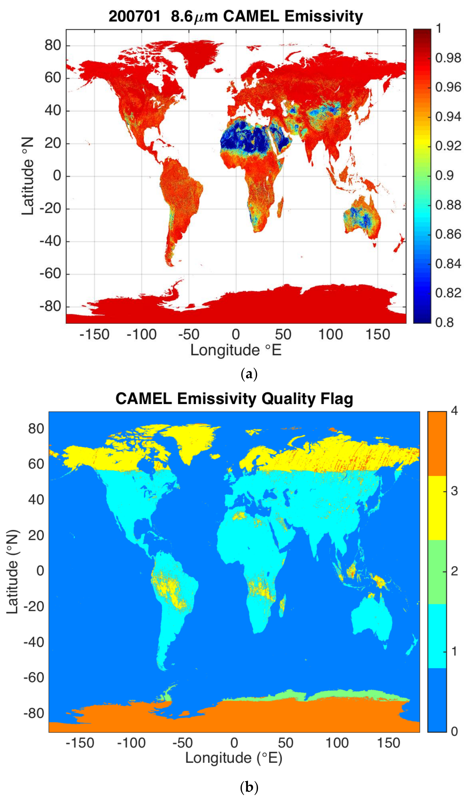
Figure 1 shows a global map of the CAMEL 8.6 µm emissivity for January 2007. Located within the quartz doublet region, this channel’s emissivity highlights the location of surface types dominated by quartz, for example the Sahara Desert, Namib Desert, and inland Arabian Peninsula. The associated CAMEL quality flag (qf), defined in Table 3, is also shown in Figure 1 and shows where no CAMEL emissivity values are reported over sea/inland water (qf = 0), where the input UW BF and ASTER data are good quality (qf = 1), the input UW BF is good quality and ASTER is filled (qf = 2), the input UW BF is filled but ASTER is good quality (qf = 3), and both the UW BF and ASTER values are filled (qf = 4). The distinct line over which the quality flag changes at ~55°N latitude is an artifact of the day/night emissivity method of the NASA MOD11C product which is used as input to the UW BF product [16]. A lack of MODIS data is also seen over land in the ~0–20°S tropical belt in regions dominated by persistent cloudiness. The north-to-south stripes over Siberia are caused by the cloudiness over the whole month in the ASTER dataset. For these cases, both datasets use filling techniques from the average of the neighboring months or annual data.
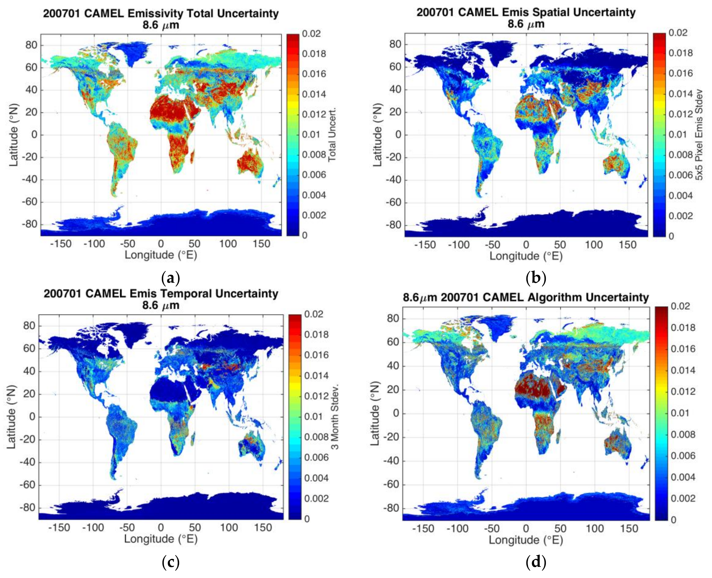
The CAMEL uncertainty product for the 8.6 µm channel during January 2007 is shown in Figure 2. The total uncertainty is shown with its quality flag and three separate uncertainty components. Qualitatively it is apparent how the total uncertainty is a combination of the three components, with the largest contributions coming from the algorithm component. The amount each component contributes to the total value varies with season. For example, the month of July in general has lower algorithm uncertainty and the spatial and temporal uncertainty has increased values north of ~60° latitude which are more readily identified as contributing to the total uncertainty. A line of larger uncertainty values is seen along the ~55°N latitude region in Asia, which is a pattern present in all 3 uncertainty components, and is attributable to the change of CAMEL input data (no UW BF input) as shown in Figure 1’s quality flag.
A comparison of the 8.6 µm spatial uncertainty to the monthly mean emissivity in Figure 1 shows areas of spatially uniform emissivity have low spatial uncertainties, for example densely vegetated regions of the Congo Forest, and persistent snow/ice covered regions of Antarctica and areas over Northern Hemisphere winter snow covered areas (northern Arctic Circle). Due to the large difference in the 8.6 µm emissivity between quartz and non-quartz surfaces, even a small mixing of surface types can yield larger spatial uncertainty values. The map of temporal uncertainty reveals that desert regions such as the Sahara, and more permanently snow-covered regions like Antarctica and the Arctic Circle are characterized by low temporal uncertainty. The northeastern United States is marked by a higher, ~0.01 temporal uncertainty likely due to changes in snow cover over the winter months, and areas around the Indus River Valley and northern India are marked by higher uncertainties likely due to changing precipitation and meltwater levels. Such patterns in the uncertainty values reveal physical characteristics and changes of the Earth’s surface. The algorithm uncertainty, which is proportional to the UW BF 8.3 µm minus ASTER 8.6 µm emissivity, shows the largest values of over 0.02, mostly over semi-arid and arid regions that exhibit the largest variability in emissivity for this band. This is due to larger differences between retrieved emissivity in this band from the ASTER and MODIS input products. However, because of ASTER’s greater number of bands in this region (3), the derived CAMEL emissivities should be of higher accuracy than the original UW BF value, which only has one band in this region. Uncertainty values over northern Russia and Canada show larger values of ~0.01 where snow cover signatures vary between the ASTER and the UW BF products.
4. Validation with Laboratory Spectra
4.1. Field Sites
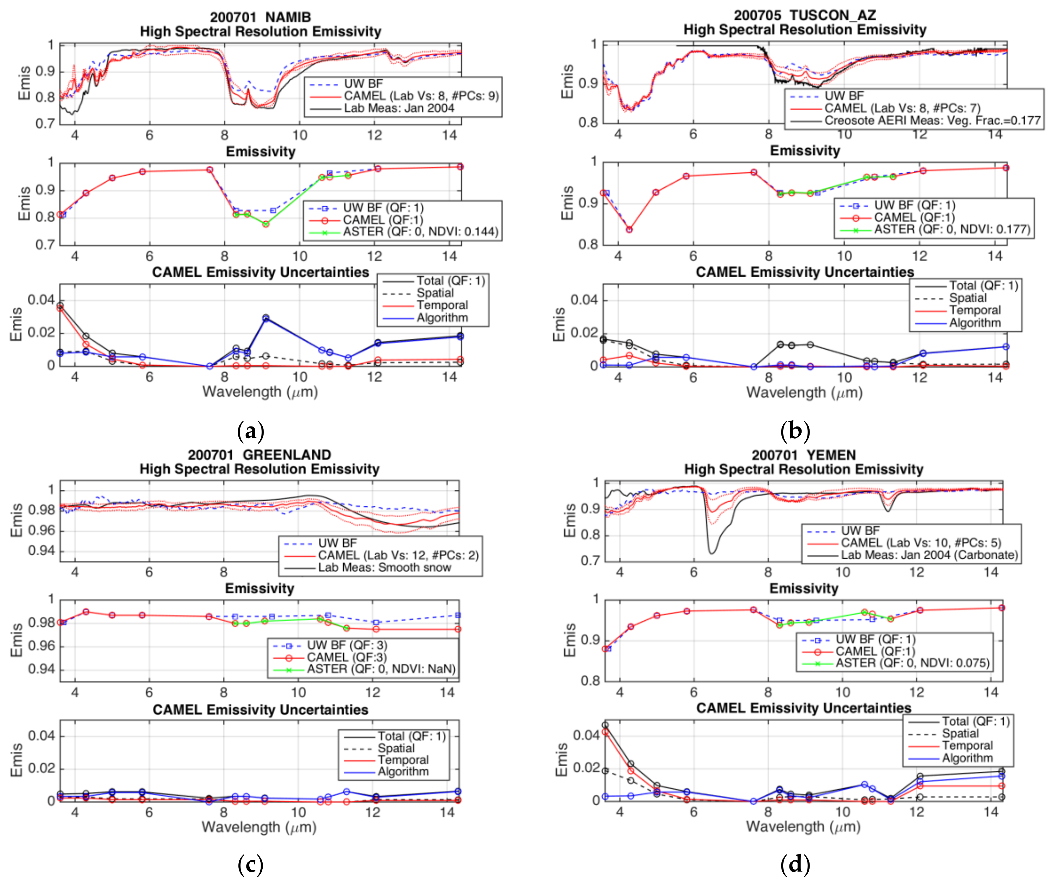
Figure 3 shows the HSR and 13 hinge point CAMEL products overlaid with the UW BF, ASTER, and lab measurement emissivities for four validation sites. The total HSR uncertainty estimate for the CAMEL HSR product is overlaid in the top panel (plotted as red dotted lines), and the CAMEL 13 hinge point total uncertainty with its 3 components are shown separately in the bottom panel.
The first site in Figure 3a shows emissivity spectra comparisons over the Namib desert during January 2007. The quartz doublet feature can clearly be seen at 8.5 and 12.5 µm since the desert sands consists mostly of quartz and hematite. In the top panel, the CAMEL HSR product closely captures the depth of the quartz doublet within the 8–9 µm region. The middle panel shows how the CAMEL emissivity is defined using ASTER bands within this 8–9.3 µm window. The difference between the ASTER and UW BF product around 9 µm is reflected in the CAMEL algorithm uncertainty shown in the bottom panel. With an exception for wavelengths less than ~5 µm where the temporal uncertainty is the largest component, the total uncertainty is dominated by the algorithmic uncertainty.
The second site shown in Figure 3b is for Tucson, Arizona in May 2007. The spectrometer data for this case was obtained from AERI in situ measurements of a characteristic creosote site, where the Creosote bush is the dominant vegetation type [14]. The ASTER NDVI is used as a vegetation fraction to form a weighted emissivity measurement from bare and vegetated spectra. This site shows very close agreement between ASTER, UW BF, and CAMEL products. This close agreement, in addition to the lack of temporal variation of the surface characteristics for wavelengths under 11 µm, produces a total CAMEL uncertainty that is mostly driven by the spatial variability of the region. While the CAMEL HSR product closely resembles the UW BF HSR emissivity across most of the spectrum, the CAMEL HSR product is more accurately able to capture the 8–9.3 µm subtle quartz feature seen in the lab validation data.
The third site in Figure 3c shows results for a site in Greenland, Summit Station, for January 2007. The top panel shows that the CAMEL HSR emissivity more accurately fits the lab data for smooth snow than does the UW BF, particularly for snow features in the 11–14 µm region. Snow spectral features are better captured because the CAMEL HSR for snow is derived from a unique set of principal component (PC) coefficients derived from laboratory spectra of different snow grain sizes, ice, and water, more details of which can be found in Part 1. While the CAMEL HSR uncertainty is around 0.01 for wavelengths over 11 µm, the 13 hinge point CAMEL uncertainty is confined well under 0.01 and is dominated by algorithm variability.
The last case site example in Figure 3d is for Yemen in January 2007. Lab measurements are derived from the ASTER spectral library and illustrate the primary carbonate features that are seen over regions of Yemen and Oman at the southern tip of the Arabian Peninsula. The CAMEL 13 hinge point product is unable to resolve the narrow 6–7 µm main carbonate feature because MODIS does not have any bands covering that region; however, the CAMEL HSR emissivity is able to capture the feature since a unique set of PC coefficients for carbonate minerals are used. The CAMEL is an improvement upon the UW BF HSR in this region since the UW BF uses only one set of PC coefficients for all surface types. Though the lab data does not lie within the bounds of the CAMEL HSR uncertainty within the ~6–7 and 11–11.5 µm regions, it is important to note that the lab spectra are a pure carbonate (dolomite) and CAMEL is representative of a 5 km pixel which likely contains a mixture of material, not purely carbonate. Additionally, the HSR uncertainty does appropriately reflect the increased difference between the CAMEL HSR emissivity and the lab validation data. Like the Namib Desert site, the Yemen desert site also has a higher CAMEL uncertainty in the shortwave region due to an increased temporal variability but otherwise is dominantly influenced by the algorithm uncertainty component.
Each of the four case sites represents a different surface type and uses a different number of PCs in the CAMEL HSR emissivity construction. The Namib Desert and Tucson, AZ cases represent surfaces characterized by quartz. Within the quartz signature region located at ~8–10.5 µm, CAMEL and the lab measurements agree within 0.05 for the Namib case and within 0.025 for the partially vegetated Tucson, AZ case. At wavelengths greater than 10.5 µm, CAMEL and the lab data agree within 0.01 for both sites, while for the Namib SW region from 3.6–6 µm, CAMEL has departures of ~0.1 magnitude away from the lab measurements. This could be explained by surface roughness and terrain elevation changes present in the satellite observation but not in the lab measurement. The Greenland case site illustrates the CAMEL snow/ice emissivity performance: for wavelengths greater than or less than 8 µm, CAMEL and the lab data agree within 0.005 and 0.01 respectively. The Yemen site characterizes the carbonate surfaces and shows the 6.5 µm spectral feature is included in the CAMEL dataset but the lab data differs by up to 0.15, with the lab measurement lying outside of the CAMEL HSR uncertainty bounds. The reduced spectral contrast in the CAMEL estimate could be explained by surface roughness or sparse vegetation not accounted for in the lab measurement.
4.2. CAMEL Intercomparison with IASI Emissivity
This section shows a comparison of CAMEL to the 8-year averaged IASI HSR emissivity dataset, which is derived from IASI radiance observations and uses a retrieval method based on Principle Component Analysis (PCA) of lab spectra [5]. To facilitate the comparison at the 13 CAMEL hinge points, the CAMEL 13 hinge point product is first resampled to a lower spatial resolution by applying a 5 × 5 pixel running average over the CAMEL grids to match the 0.25° × 0.25° spatial resolution of the IASI dataset. CAMEL 8-year averaged monthly emissivities are then computed corresponding to the years over which the IASI dataset is averaged. For the months of January through May the years 2008–2015 are averaged, and for June through December the years of 2007–2014 are averaged. To compare the HSR CAMEL product to the HSR IASI emissivity, the individual CAMEL HSR spectra are simply computed and averaged over the proper years. Since the CAMEL HSR 8-year monthly averages actually represent a 0.05° × 0.05° resolution, the HSR uncertainty estimate, which includes a measure of the surrounding 0.25° × 0.25° standard deviation, is used to provide a measure of the potential error from the spatial resolution mismatch (i.e., of the CAMEL 0.05° × 0.05° to the IASI 0.25° × 0.25°).
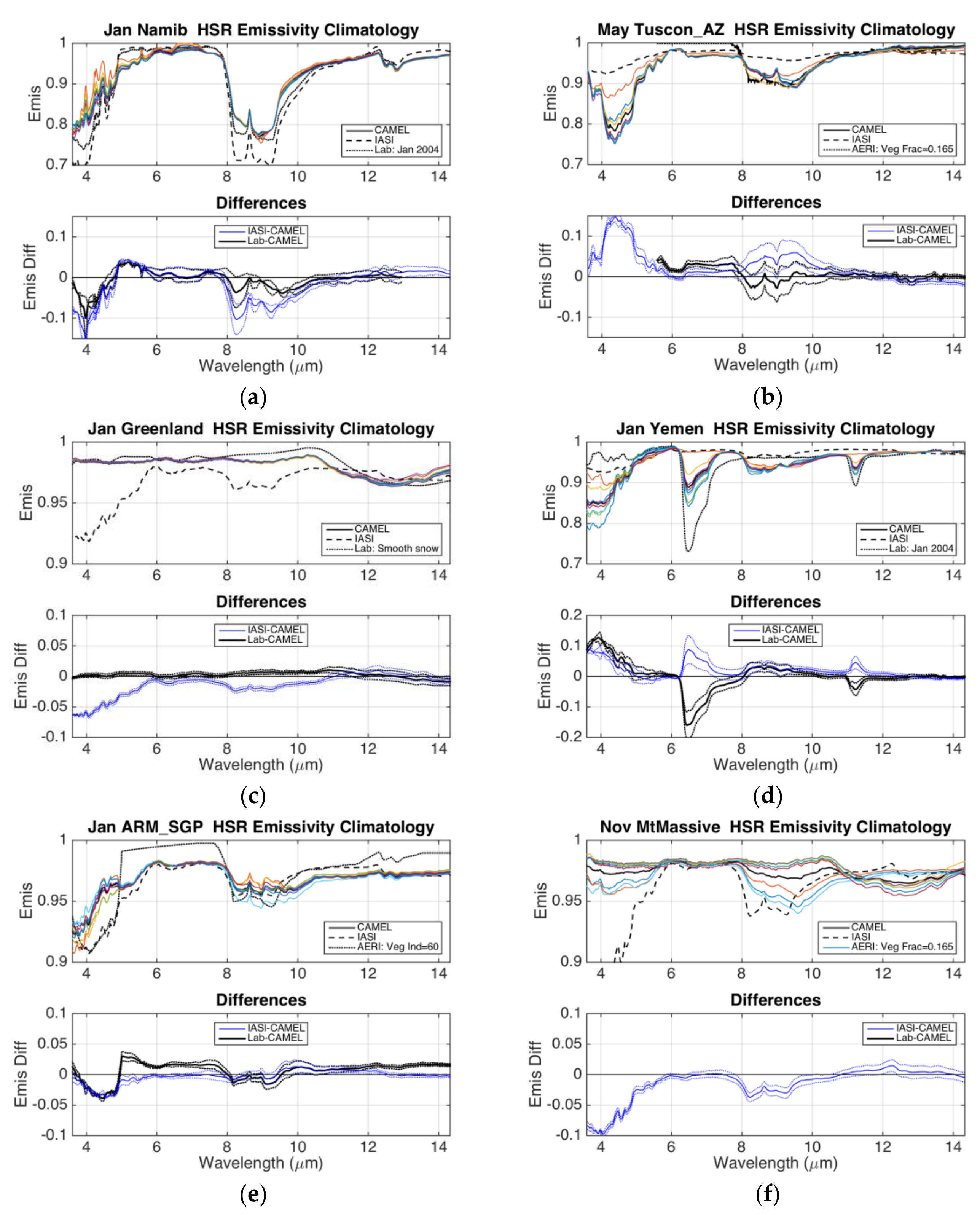
Figure 4 shows the monthly 8-year averages of CAMEL HSR emissivities compared against (i) laboratory validation data (where it is available) and (ii) the IASI HSR dataset for various case sites. The 8-year averaged HSR emissivities are overlaid in the top panels, including individual CAMEL spectra for each of the years averaged, and the bottom panels show the 8-year average differences bounded by the CAMEL uncertainty estimate. At the top of Figure 4, the Namib and Tucson, AZ desert cases show emissivity differences between the CAMEL and lab emissivities of less than 0.05 for wavelengths greater than 5 µm. Within the quartz spectral region, CAMEL agrees more closely with the lab measurements than the IASI emissivity. For the Greenland case site, differences between the lab and CAMEL emissivities are less than 0.01. The IASI emissivity reflects a subtle quartz signature which is absent in CAMEL. This case shows the importance of the selection of laboratory measurements for the PCA method. For snow or ice-covered cases the CAMEL HSR Algorithm includes a separate set of laboratory measurements of snow and ice spectra only. The Yemen case site shows the 8-year average CAMEL emissivity having a ~0.15 maximum difference from the lab measurements around the 6.5 µm carbonate spectral feature. While CAMEL does not capture the full extent of this feature as shown by the lab measurements, it is an improvement upon the UW BF and IASI emissivity, as the feature is present, but lower in magnitude. For the ARM SGP site, the CAMEL and IASI 8-year averages have close resemblance across the spectrum with the exception of the 8–9.5 µm region where IASI resolves the sharper features of the quartz signature. Differences between the CAMEL and lab emissivity are generally less than 0.025 with a small exception in the SW region at 5 µm. The last case site (no lab validation data is available) over Mt. Massive, located in the Colorado Rocky Mountains, is shown for the month of November. The overlaid November CAMEL HSR estimates for the years 2007–2014 located in the top panel reveal the year to year variation which is captured by the monthly CAMEL product. In some years, HSR emissivities reflect snow/ice signatures (version number of the laboratory dataset: Vs = 12 and #PC = 2), while others reflect more quartz-like signatures of bare rocks (Vs = 8 and #PC = 7), reflecting the dynamics of annual snow cover and snow-melt across the region.
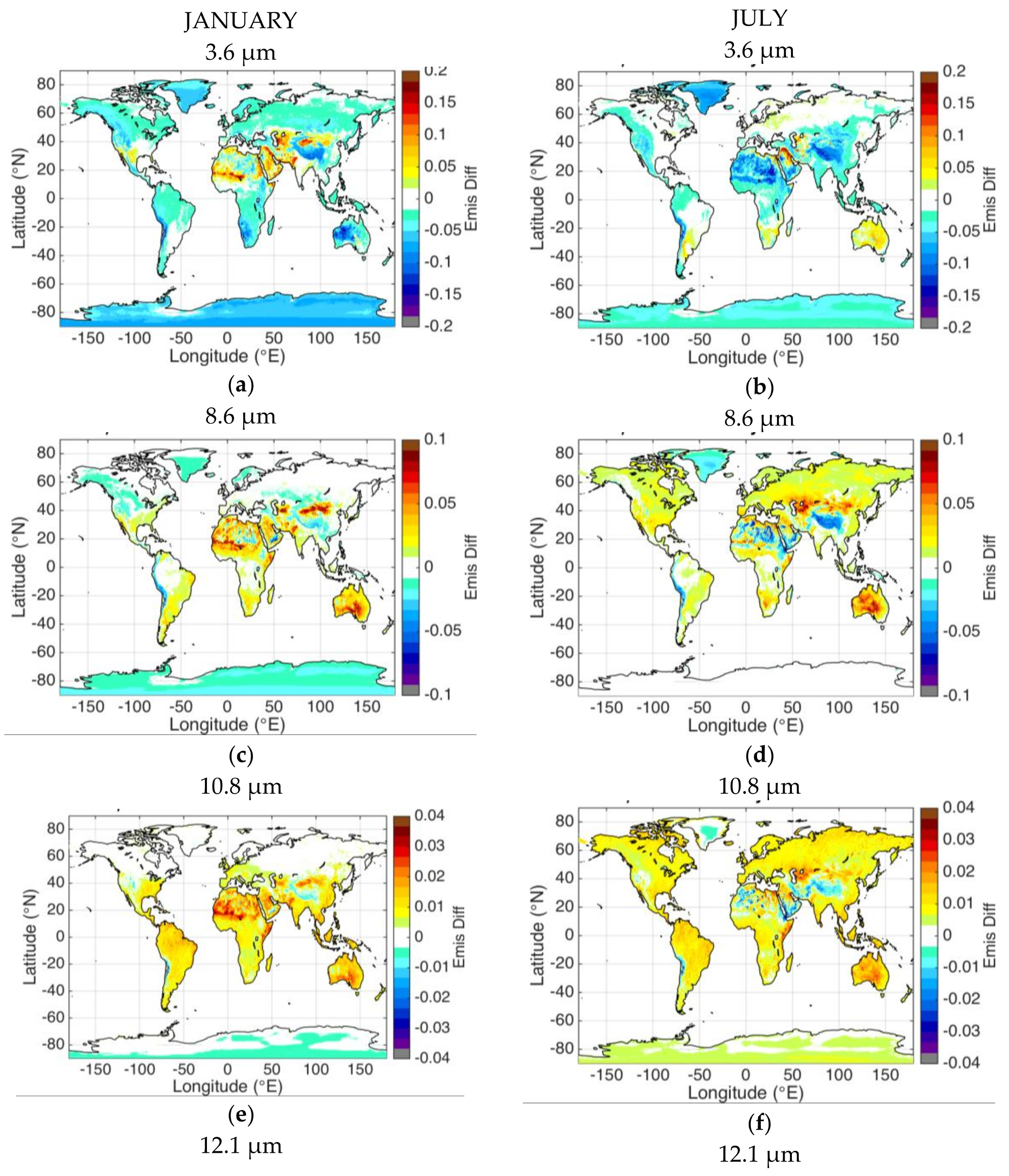
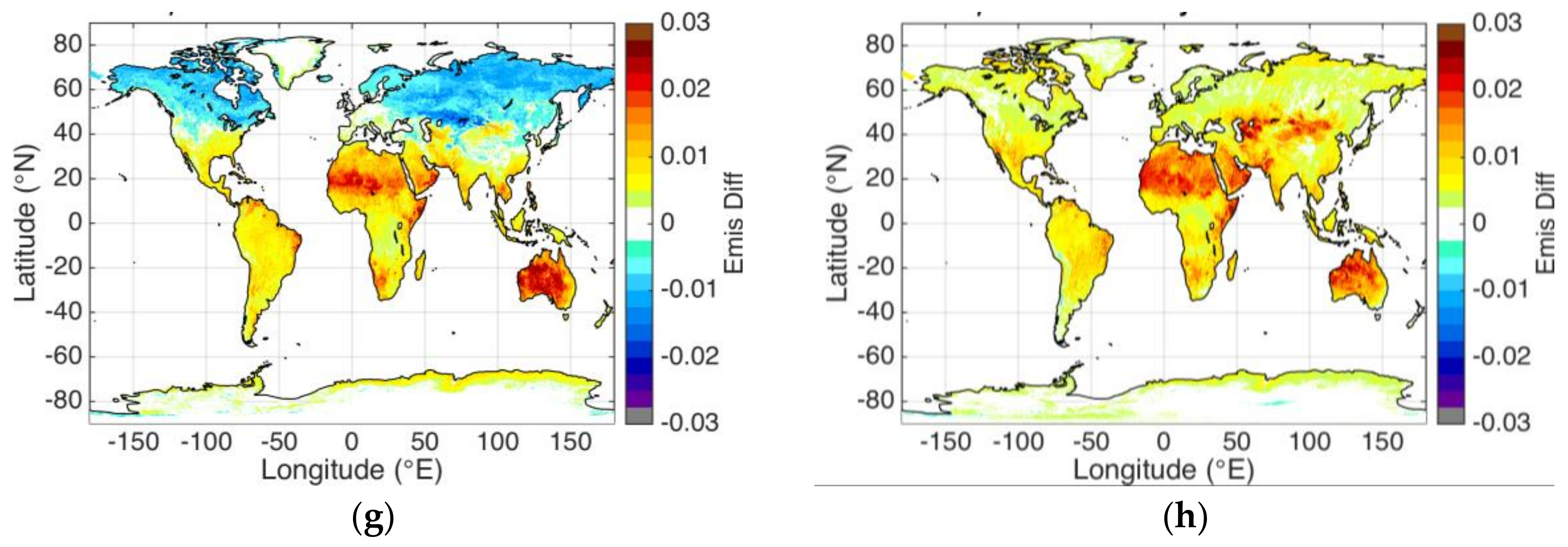
Figure 5 shows global maps of the differences between the CAMEL and IASI 8-year averages for the months of January and July at 4 different wavelengths. The global maximum magnitude of differences is larger for the shortwave and 8–9 µm channels (e.g., the 3.6 and 8.6 µm channels), where differences exceed 0.1 in select places (e.g., Sahara Desert, Australia, Tibetan Plateau), typically in regions whose surfaces are barren. Comparison of the January and July results reveals a seasonal dependence in the differences for various regions and channels, seen most notably at high latitudes where snow cover varies with the seasons. In general, a stable emissivity over deserts and polar ice (Greenland and Antarctica) is expected, so the large IASI variations over deserts and polar ice is unphysical and synthetic. The IASI emissivity over permanent snow cover contains quartz signature artifacts as discussed previously. The 10.8 µm channel shows slight changes from January to July and does show select areas where CAMEL emissivity is higher than IASI such as over the Tibetan Plateau, but in general CAMEL emissivities are lower than IASI at 10.8 µm. The 12.1 µm channel shows that for latitudes south of ~40°N where there is no snow cover, that the IASI minus CAMEL 8-year average difference is qualitatively similar between January and July and is largely positive, though it is quite small, being confined to under 0.03 magnitude.
Statistics of the 8-year averaged IASI minus CAMEL emissivity over IGBP land classification categories are shown in Figure 6 for the months of January and July. Top panels show the average IASI and CAMEL emissivities and the bottom panel shows the average IASI minus CAMEL difference. Differences are generally less than a magnitude of 0.02 in emissivity and could be due to multiple issues including differences of spatial resolution between the IASI and MODIS/ASTER instruments and differences between the IASI emissivity and CAMEL algorithms. While differences could also be due the assumption of equal emissivity over day and night, further investigation is needed on this topic. Largest differences between the CAMEL and IASI products are seen in the barren/sparse vegetation category, where they exceed 0.03 in magnitude. The IASI product has larger differences between January and July than CAMEL does for the barren/sparse 8–11 µm region. But the CAMEL product has larger differences between January and July in the grassland 8–11 µm region. The CAMEL temporal variations over temperate grasslands and stable emissivity over deserts is as expected due to changes in phenology that affect vegetation cover.
4.3. RTTOV IASI Brightness Temperature Calculations
4.3.1. Methodology
As an additional assessment of the CAMEL HSR product, IASI brightness temperatures (BT) are calculated using the RTTOV model and CAMEL HSR emissivity module for 616 selected channels (National Oceanic and Atmospheric Administration selection) for four focus days representing the four seasons including 15 January, 14 April, 15 July, and 29 September of 2008. Similar calculations are performed for a constant with wavenumber 0.98 emissivity spectrum to assess the impact of the difference between the CAMEL dataset and commonly used default 0.98 emissivity value. Both sets of calculated BTs are then compared to IASI observed radiances for a subset of cases over land (coastlines not included) and for clear sky conditions. The clear sky mask that is used is the MAIA cloud mask [17], which selects scenes with less than 95% cloud cover. Simplifications to the BT calculations include setting the satellite zenith and azimuth and sun zenith and azimuth angles to zero, not applying the snow fraction, and using no trace gas inputs besides water vapor. ECMWF 6 hourly, 0.25° spatial resolution, analyses are used as input into the RTTOV model. The model analyses are bilinearly-interpolated to the IASI observations, specifically the center of the IASI fields of view. To minimize the effect of rapid skin temperature variations on the comparisons, only nighttime cases (solar zenith angles greater than 85°) are used and a two-hour time restriction between IASI observations and ECMWF analyses time steps is applied.
4.3.2. Results
Differences between the calculated and observed IASI BTs are computed over the 616 channel set and separated by land classification type using the IGBP categories. The improper skin temperature determination can cause a bias in the BT calculation. This bias between ECMWF and IASI has a magnitude typically around 1–2 K in the Northern Hemisphere and 2–3 K in the Southern Hemisphere. To avoid it the de-biased variances of the calculated minus observed BTs differences for the 3.6–5, 8–9, and 10–13 µm spectral regions are used as indicators for a better emissivity estimate. To compute the de-biased variances for each spectrum, the IASI BT calculation minus observation difference is found and the result is then fitted to the 10.5–13 µm window region by subtracting the calculation minus observation 10.5–13 µm spectral domain average from the calculated spectrum. This de-biasing using the window region is assumed to only account for differences in skin temperature, though it’s possible that the de-biasing could account for other errors of lesser magnitudes such as inaccurate surface emissivity characterization and errors induced from the inclusion of cloudy scenes in the analysis. Three separate spectral variances over the 3.6–5, 8–9, and 10–13 µm regions are then computed for the window-fitted BT difference. Using this method, there are 3 separate variances computed for each IASI calculation. The de-biased variance statistics corresponding to the CAMEL and 0.98 emissivity are compared for different time and space domains by taking averages of the variances over the specific regions.
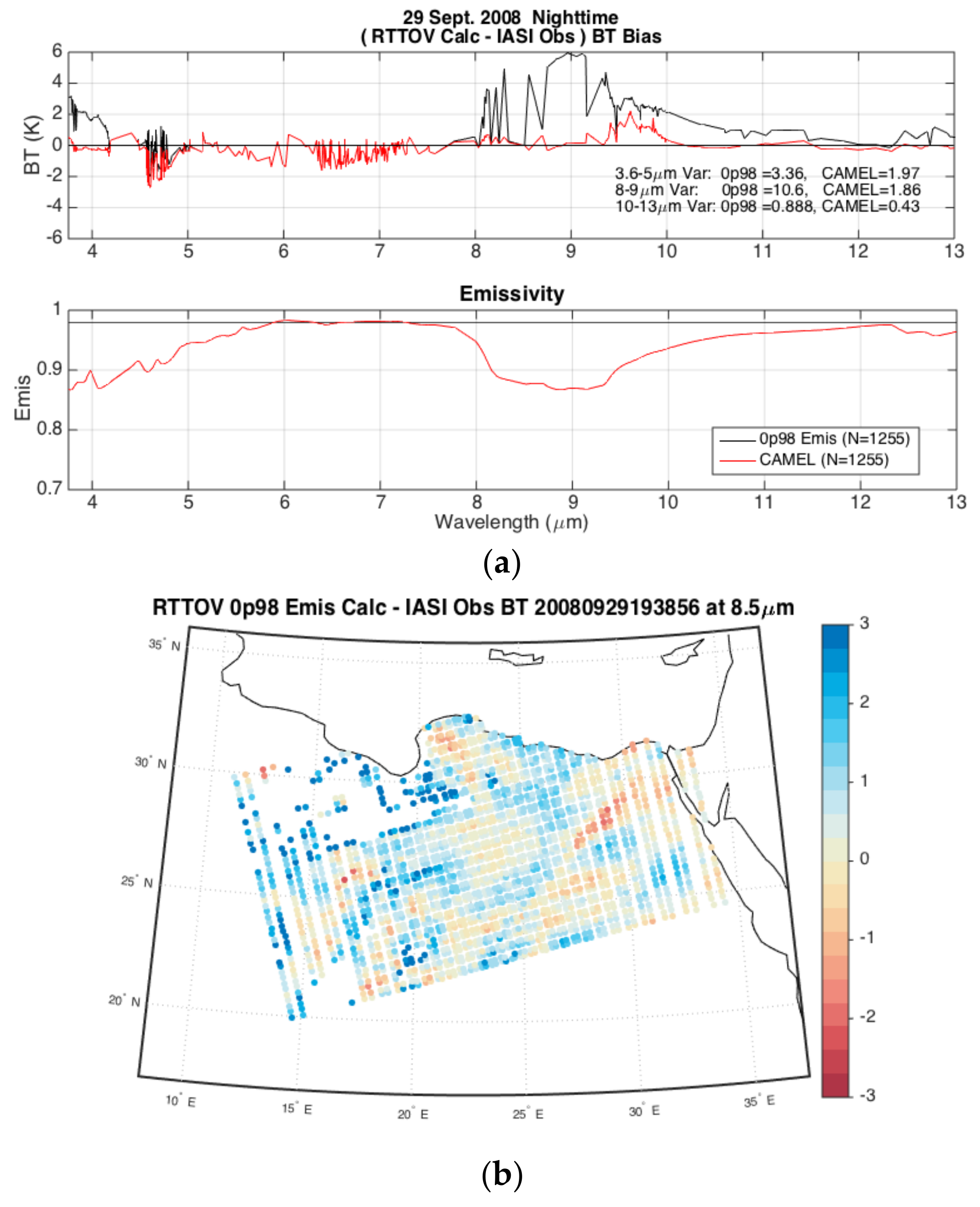
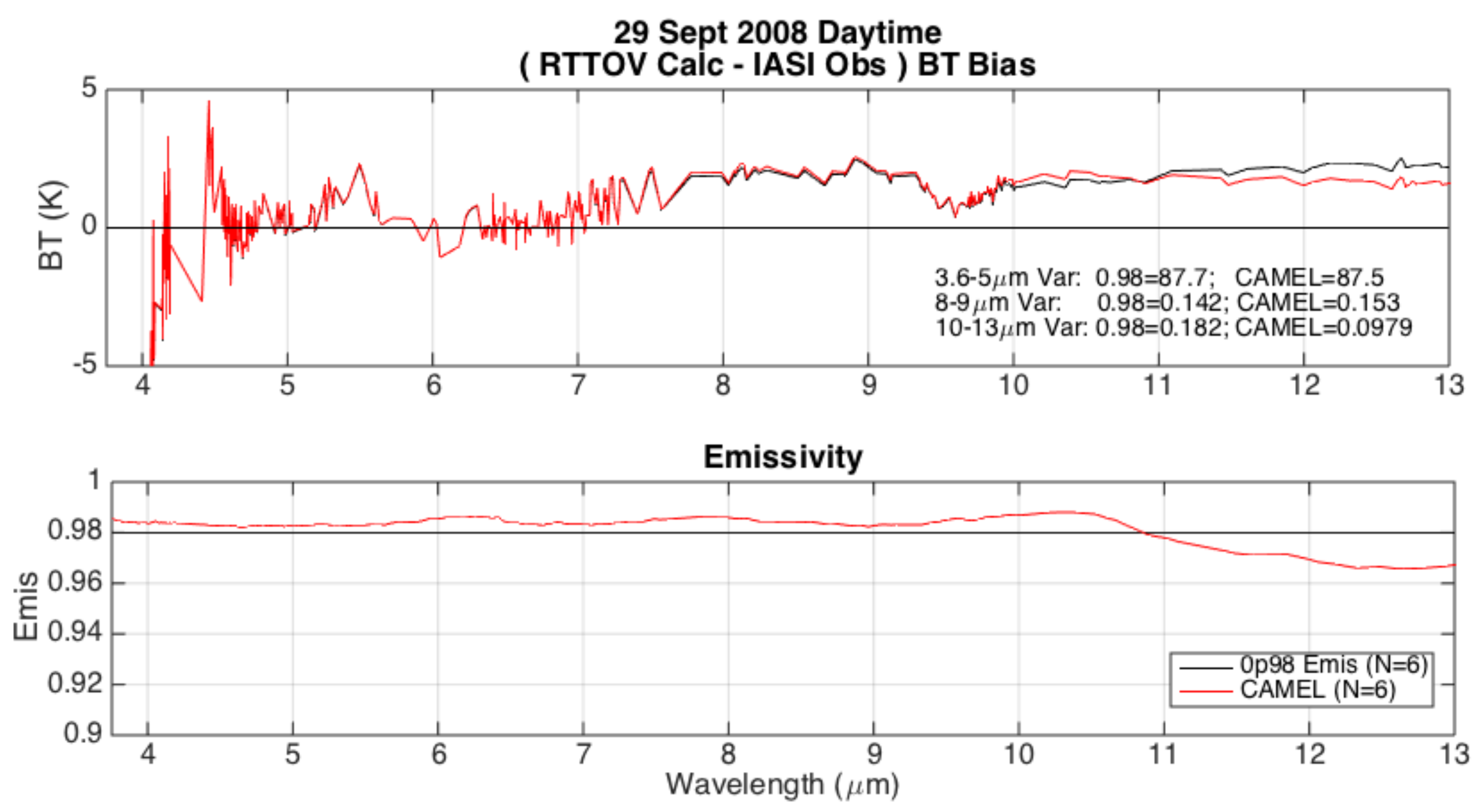
Figure 7 shows mean CAMEL and 0.98 constant emissivity spectra and calculated minus observed IASI BT biases for a nighttime granule over Egypt. The 8.5 µm map of the calculated CAMEL minus observed BTs illustrates the spatial distribution and magnitude of the differences. This example shows the very large improvement of over 5 K when using CAMEL emissivity as opposed to the constant 0.98 emissivity value within the 8–10 µm region Reststrahlen band region. De-biased variance values over the three spectral regions can be found in the upper panel and show lower, improved values for the CAMEL dataset. The CAMEL calculated minus observed BT bias has increased magnitudes in spectral regions where atmospheric gases strongly absorb, in particular the 4.5–5 µm carbon monoxide and carbon dioxide region, the 6–8 µm water vapor region, and 9.6–10 µm ozone absorption region. Figure 8 shows a second nighttime example of statistics from a granule over the coast of Antarctica. Though not many samples are included in this granule, results are representative of snow and ice scenes. The BT bias corresponding to the CAMEL emissivity calculations is greater than the 0.98 emissivity bias from approximately 10–10.8 µm, however, it is less within the ~11–13 µm region where most of the spectral variation in snow/ice emissivity occurs. The magnitude of the BT bias difference is just under 1 K and represents how the CAMEL emissivity changes with respect to the 0.98 constant emissivity in the bottom panel. While the 8–9 µm de-biased variance is greater for CAMEL than the 0.98 constant, the 10–13 µm value is overall decreased.
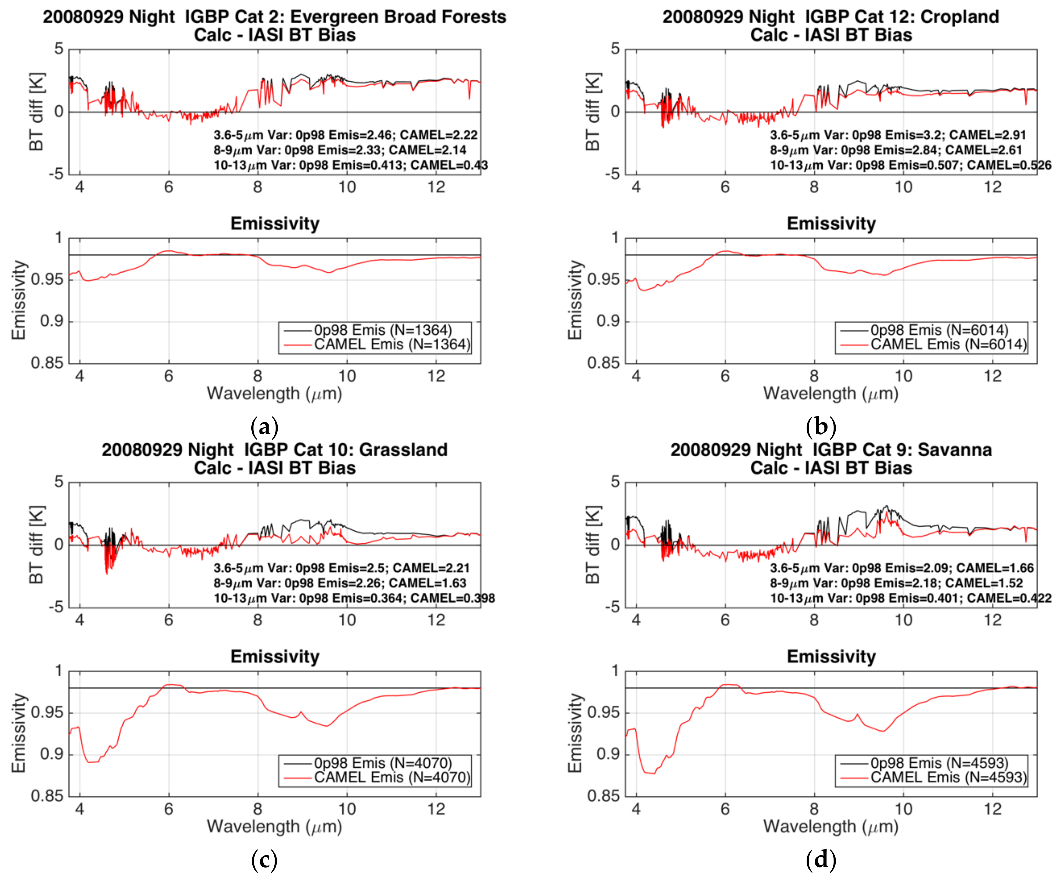
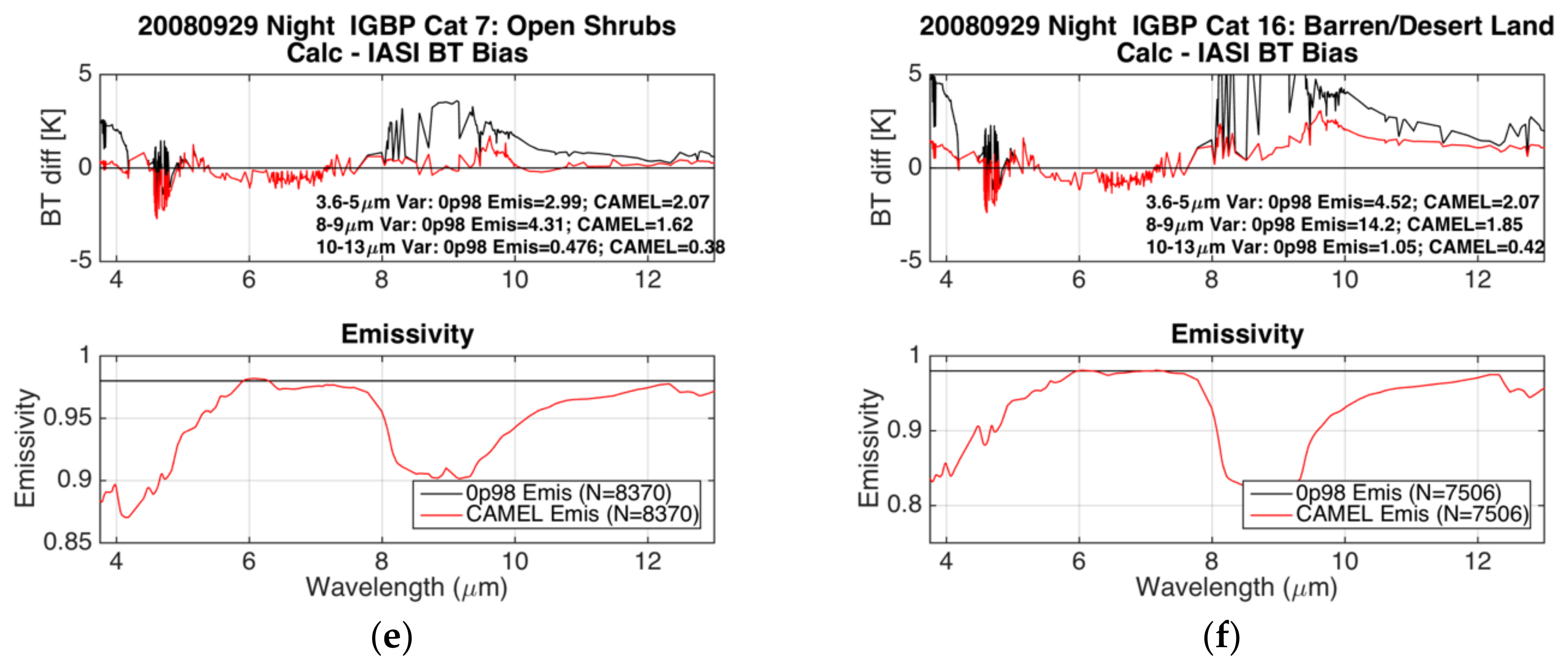
Figure 9 shows nighttime statistics of the calculated minus observed IASI BTs for various IGBP land classification categories for the 29 September 2008 case day. While these examples are not comprehensive of all days and seasons, some general characteristics can be seen. For all categories shown, the CAMEL calculated BT is seen to generally be closer to the observed IASI BT than the 0.98 emissivity calculated BT. Land classification categories with emissivity spectra close to 0.98, such as the evergreen broad-leaf forests and croplands show the smallest bias difference between the CAMEL and 0.98 emissivity BT calculations. Largest differences are seen in the barren/desert land category around 8–9.5 µm, where the emissivity spectra have prominent quartz spectral features and reach values less than 0.7, as expected. The CAMEL calculations also show better agreement with the observations than the 0.98 emissivity calculations within the 3.6–4.2 µm region. Improved agreement around these wavelengths is seen for all other land categories shown as well. Comparison of the de-biased variance statistics for the CAMEL and 0.98 emissivity also confirms that for all land categories shown the CAMEL HSR emissivity is a spectral improvement upon the constant 0.98 emissivity within the 3.6–5 and 8–9 µm region. The 10–13 µm region de-biased variance statistics show neutral improvement using the CAMEL emissivity for all categories shown except for the open shrub and barren/desert land category where reductions in variance are significant.
To summarize the global RTTOV calculated minus observed statistics over the 4 case days, the CAMEL and 0.98 emissivity de-biased variances are listed for the 8–9 µm spectral region in Table 4. While variances for the 10–13 and 3.6–4.2 µm regions were calculated in a similar fashion, the results are not listed here and are only discussed qualitatively. The 8–9 µm region was selected to be shown since this spectral region is the region of largest expected improvement in comparison to the previous UWIREMIS. The numbers shown in Table 4 are averages of de-biased variances for the focus days and IGBP land classification categories shown. The corresponding number of samples are illustrated in Figure 9.
Table 4 results show in general that CAMEL is an improvement upon the 0.98 constant emissivity for this spectral region. For all categories with over 2000 samples, the CAMEL de-biased variance is lower than the 0.98 emissivity de-biased variance. The open shrub and barren/desert land categories again show the largest percent decreases in de-biased variance from the 0.98 emissivity to CAMEL. The CAMEL de-biased variance is decreased on average for the four days to ~41% and ~21% of the 0.98 emissivity value respectively for the open shrub and barren/desert land categories.
In addition to the 8–9 µm region, the 3.6–5 µm region of CAMEL also better matches the IASI observations than does the 0.98 constant emissivity. De-biased variances for CAMEL are overall lower than those for the 0.98 constant emissivity in the 3.6–5 µm region, with the exceptions being for cases with a low (e.g., less than 100) number of samples. The open shrub and barren/desert categories showed the most CAMEL improvement—the de-biased variances for CAMEL are decreased respectively to be ~79% and ~56% of the 0.98 emissivity de-biased variance.
The last spectral region assessed, the 10–13 µm region, does not show an obvious improvement with the use of the CAMEL. For the average of the four case days, more land classifications show an increase, rather than a decrease, in the CAMEL de-biased variances. Improvement is seen, however, in the barren/desert land and open shrub categories, with the average CAMEL variances being 52% and 80% of the 0.98 variance respectively. The deciduous needle forest and mixed forest categories have the largest average increases of 10–13 CAMEL de-biased variances with respect to the 0.98 values, with 15% being the largest increase.
5. Conclusions
The NASA CAMEL product reports monthly global land surface emissivity at 13 hinge points between 3.6–14.3 µm and provides software which uses a PCA approach to compute 417 channel high spectral emissivity spectra from the 13 hinge point product for the same wavelength region. The uncertainty provided with the product is available at the 13 hinge point resolution for every month and grid point and is a combination of 3 separate components of variability—a spatial, temporal, and algorithm component. This work presented the methodology behind the uncertainty estimates included in the product and a comprehensive validation of the CAMEL product which included laboratory measurements, product intercomparisons, and radiative transfer calculations.
Comparisons of CAMEL to validation data, the 8-year averaged IASI dataset, and the previous UW BF emissivity show an improvement of CAMEL in the characterization of snow, quartz, and carbonate spectral features. The monthly and inter-annual variations of the emissivity reveal dynamic land surface changes, for example, snow in the mountains. Comparison of the CAMEL 13 hinge point product to the 8-year averaged IASI dataset at 0. 25° spatial resolution showed maximum differences were located in the shortwave 3.6 µm region, where they reached over 0.15 magnitude in emissivity for some geographic locations, typically dry desert regions. Differences at 8.6 µm were primarily less than 0.1 and at wavelengths of 10.8 µm or larger they were predominantly under 0.02.
Assessment of the CAMEL RTTOV emissivity module was made using IASI brightness temperature observations as a reference. Calculated minus observed BT biases were computed for both the CAMEL emissivity and a constant 0.98 emissivity spectra, a commonly used simplification for a land surface emissivity estimate. The use of a de-biased spectral variance over three spectral regions was used as a measure of emissivity spectral accuracy. The average of the de-biased variances was found over IGBP land classification schemes for four days which represented four seasons. Land classifications which showed improvement with the use of the CAMEL emissivity for all three spectral regions were the open shrub and barren/desert land categories. In general, the 3.6–5 and 8–9 µm region statistics showed the CAMEL to be a better emissivity estimate than the constant 0.98 value, while the 10–13 µm region showed an improvement only for barren or partially barren surfaces. As expected, the percentage decreases in the 3.6–5 and 8–9 µm four day-averaged variances were larger than the percent increases for the 10–13 µm region when comparing CAMEL with respect to the 0.98 emissivity.
This two-part paper has described the methodology, applications, uncertainty, and validation of the first release of the CAMEL dataset available from a NASA MEASUREs project at https://lpdaac.usgs.gov/dataset_discovery/measures/measures_products_table/cam5k30em_v001. Future work will include version updates to improve some known issues, for example, snow fraction in mixed scenes, and the development of a 16-year CAMEL climatology and covariance for use in NWP applications.
Acknowledgments
The ASTER GED version 4 (v4) product used in this study was produced at JPL and is available courtesy of the NASA EOSDIS Land Processes Distributed Active Archive Center (LP DAAC), United States Geological Survey/Earth Resources Observation and Science Center, Sioux Falls, South Dakota, [https://lpdaac.usgs.gov/dataset_discovery/aster]. This work was done under grant number: NNX08AF8A.
Conflicts of Interest
The authors declare no conflict of interest.
References
- Seemann, S.W.; Borbas, E.E.; Knuteson, R.O.; Stephenson, G.R.; Huang, H.-L. Development of a Global Infrared Land Surface Emissivity Database for Application to Clear Sky Sounding Retrievals from Multispectral Satellite Radiance Measurements. J. Appl. Meteorol. Climatol. 2008, 47, 108–123. [Google Scholar] [CrossRef]
- Hulley, G.C.; Hook, S.J.; Abbott, E.; Malakar, N.; Islam, T.; Abrams, M. The ASTER Global Emissivity Dataset (ASTER GED): Mapping Earth’s emissivity at 100 meter spatial scale. Geophys. Res. Lett. 2015, 42, 7966–7976. [Google Scholar] [CrossRef]
- Saunders, R.; Hocking, J.; Rundle, D.; Rayer, P.; Havemann, S.; Matricardi, M.; Geer, A.; Cristina, L.; Brunel, P.; Vidot, J. RTTOV-12 Science and Validation Report; EUMETSAT NWP SAF, NWPSAF-MO-TV-41; EUMETSAT: Darmstadt, Germany, 2017. [Google Scholar]
- Borbas, E.E.; Ruston, B.C. The RTTOV UWiremis IR Land Surface Emissivity Module; EUMETSAT NWP SAF, NWPSAF-MO-VS-042; EUMETSAT: Darmstadt, Germany, 2010. [Google Scholar]
- Zhou, D.K.; Larar, A.M.; Liu, X. MetOp-A/IASI observed continental thermal IR emissivity variations. IEEE J. Sel. Top. Appl. Earth Obs. Remote Sens. 2013, 6, 1156–1162. [Google Scholar] [CrossRef]
- Zhou, D.K.; Larar, A.M.; Liu, X.; Smith, W.L.; Strow, L.L.; Yang, P.; Schlussel, P.; Calbet, X. Global land surface emissivity retrieved from satellite ultraspectral IR measurements. IEEE Trans. Geosci. Remote Sens. 2011, 49, 1277–1290. [Google Scholar] [CrossRef]
- Friedl, M.A.; Sulla-Menashe, D.; Tan, B.; Schneider, A.; Ramankutty, N.; Sibley, A.; Huang, X. MODIS Collection 5 global land cover: Algorithm refinements and characterization of new datasets. Remote Sens. Environ. 2010, 114, 168–182. [Google Scholar] [CrossRef]
- Channan, S.; Collins, K.; Emanuel, W.R. Global Mosaics of the Standard MODIS Land Cover Type Data; University of Maryland and the Pacific Northwest National Laboratory: College Park, MD, USA, 2014. [Google Scholar]
- Hook, S. Combined ASTER and MODIS Emissivity for Land (CAMEL) Uncertainty Monthly Global 0.05Deg V001 [Data set]. NASA EOSDIS L. Process. DAAC 2017. [Google Scholar] [CrossRef]
- Gillespie, A.; Rokugawa, S.; Matsunaga, T.; Steven Cothern, J.; Hook, S.; Kahle, A.B. A temperature and emissivity separation algorithm for advanced spaceborne thermal emission and reflection radiometer (ASTER) images. IEEE Trans. Geosci. Remote Sens. 1998, 36, 1113–1126. [Google Scholar] [CrossRef]
- Borbas, E.E.; Knuteson, R.O.; Seemann, S.W.; Weisz, E.; Moy, L.A.; Huang, H.-L. A high spectral resolution global land surface infrared emissivity database. In Proceedings of the Joint 2007 EUMETSAT Meteorological Satellite Conference and the 15th Satellite Meteorology & Oceanography Conference of the American Meteorological Society, Amsterdam, The Netherlands, 24–28 September 2007. [Google Scholar]
- Baldridge, A.M.; Hook, S.J.; Grove, C.I.; Rivera, G. The ASTER spectral library version 2.0. Remote Sens. Environ. 2009, 113, 711–715. [Google Scholar] [CrossRef]
- Dozier, J.; Warren, S.G. Effect of viewing angle on the infrared brightness temperature of snow. Water Resour. Res. 1982, 18, 1424–1434. [Google Scholar] [CrossRef]
- Knuteson, R.O.; Best, F.A.; DeSlover, D.H.; Osborne, B.J.; Revercomb, H.E.; Smith, W.L. Infrared land surface remote sensing using high spectral resolution aircraft observations. Adv. Space Res. 2004, 33, 1114–1119. [Google Scholar] [CrossRef]
- Tobin, D.C.; Revercomb, H.E.; Knuteson, R.O.; Lesht, B.M.; Strow, L.L.; Hannon, S.E.; Feltz, W.F.; Moy, L.A.; Fetzer, E.J.; Cress, T.S. Atmospheric Radiation Measurement site atmospheric state best estimates for Atmospheric Infrared Sounder temperature and water vapor retrieval validation. J. Geophys. Res. D Atmos. 2006, 111, D09S14. [Google Scholar] [CrossRef]
- Wan, Z.; Li, Z.-L. A physics-based algorithm for retrieving land-surface emissivity and temperature from eos/modis data. IEEE Trans. Geosci. Remote Sens. 1997, 35, 980–996. [Google Scholar] [CrossRef]
- Lavanant, L. MAIA AVHRR Cloud Mask and Classification; Meteo-France: Lannion, France, 2002. [Google Scholar]
Figure 1.
Combined ASTER and MODIS Emissivity over Land (CAMEL) (a) 8.6 µm emissivity and; (b) quality flag for January 2007. Quality flag is defined as in Table 3. The University of Wisconsin Baseline-Fit (UW BF) has fill values north of ~55°N congruent with the prevailing winter nighttime of January at those latitudes. This is because the MOD11C3 product used as input to UW BF is dependent on a day–night algorithm that requires a day and night observation close in time, and there is not enough daytime data in the Northern Hemisphere winter.

Figure 2.
January 2007 CAMEL 8.6 um emissivity uncertainty (a) total estimate; (b) spatial component; (c) temporal component; (d) algorithm component; and (e) total uncertainty quality flag which is defined in Table 2.
Figure 2.
January 2007 CAMEL 8.6 um emissivity uncertainty (a) total estimate; (b) spatial component; (c) temporal component; (d) algorithm component; and (e) total uncertainty quality flag which is defined in Table 2.


Figure 3.
Emissivity at (a) January 2007 Namib Desert (−24.25N, 15.25E); (b) May 2007 Tucson, AZ (32.01N, −110.77E); (c) January 2007 Greenland (72.57N, −38.45E); and (d) January 2007 Yemen (19.15N, 55.57E) case sites. HSR emissivity from UW BF (blue dashed), lab measurements (black), and CAMEL (red solid with dotted uncertainty) are shown in top row panels. UW BF (blue squares, dashed), ASTER (green x’s, solid), and CAMEL (red circles, solid) emissivity are shown in middle row panels. CAMEL total (black solid), spatial (black dash), temporal (red), and algorithm (blue) uncertainty components are shown in bottom panels. Legend in middle and bottom panel include quality flags (QF) for the different products as well as ASTER normalized difference vegetation index (NDVI). The version number (Vs) of the laboratory dataset and the number of principal components (#PCs) used in the CAMEL HSR Algorithm are included in the legend of the top panels.

Figure 4.
High spectral resolution (HSR) emissivity for (a) January Namib (−24.25N, 15.25E); (b) May Tucson, AZ (32.01N, −110.77E); (c) January Greenland (72.57N, −38.45E); (d) January Yemen (19.15N, 55.57E); (e) January Atmospheric Radiation Measurement, Southern Great Plains (ARM SGP) (36.60N, −97.48E); and (f) Nov Mt. Massive (39.17N, −106.47E) case sites. Top panels show CAMEL 8-year averaged (solid black), lab measurement (dotted black), and Infrared Atmospheric Sounding Interferometer (IASI) 8-year averaged (dashed black) HSR emissivity spectra overlaid on top of the individual CAMEL spectra for the years over which the aforementioned average was computed (colored). Bottom panel shows differences of the IASI minus CAMEL averages (blue solid) and lab minus CAMEL emissivity (black solid) which are both bounded by the CAMEL HSR uncertainty (dotted lines).

Figure 5.
Difference of IASI minus CAMEL 8-year average emissivities at 0.25° × 0.25° spatial resolution for (a) January 3.6 µm; (b) July 3.6 µm; (c) January 8.6 µm; (d) July 8.6 µm; (e) January 10.8 µm; (f) July 10.8 µm; (g) January 12.1 µm; (h) July 12.1 µm. The years for which the 8-year averages are calculated are 2008–2015 for January and 2007–2014 for July. Colorbar limits change from channel to channel.


Figure 6.
Top panels show IASI (black) and CAMEL (red) 8-year average emissivity averaged over the (a) evergreen broadleaf forest; (b) barren/sparse vegetation; (c) grassland; and (d) cropland IGBP land classifications for the months of January (solid line, circle markers) and July (red line, ‘X’ markers). Bottom panels show the associated averaged IASI minus CAMEL again for January (black dashed ‘X’ markers) and July (black solid circle markers). Number of samples, N, noted in bottom panel’s legend.

Figure 7.
(a) Calculated constant 0.98 (black) and CAMEL (red) emissivity brightness temperature (BT) minus observed IASI BT bias (top panel) and mean emissivities (bottom panel) for a 29 September 2008 nighttime granule over Egypt. Number of samples, N, shown in legend. Debiased variances listed for three spectral regions; (b) Map of 8.5 µm calculated CAMEL minus observed IASI BTs differences in Kelvin.

Figure 8.
Same as Figure 7a except for daytime granule located over the coast of Antarctica.
Figure 8.
Same as Figure 7a except for daytime granule located over the coast of Antarctica.

Figure 9.
Nighttime RTTOV calculated minus observed IASI BT biases (top panels) for a constant 0.98 emissivity (black) and the CAMEL emissivity dataset (red) with associated mean emissivity spectra (bottom panels) for 29 September 2008 for the (a) evergreen broad-leaf forest; (b) cropland; (c) grassland; (d) savanna; (e) open shrub; and (f) barren/desert land IGBP categories. De-biased variances (explanation in text) are used as the better emissivity estimate and are shown in figures. The number of samples, N, are listed in figure legends. Note that the bottom panel y-axis limits change for the desert/barren land category.


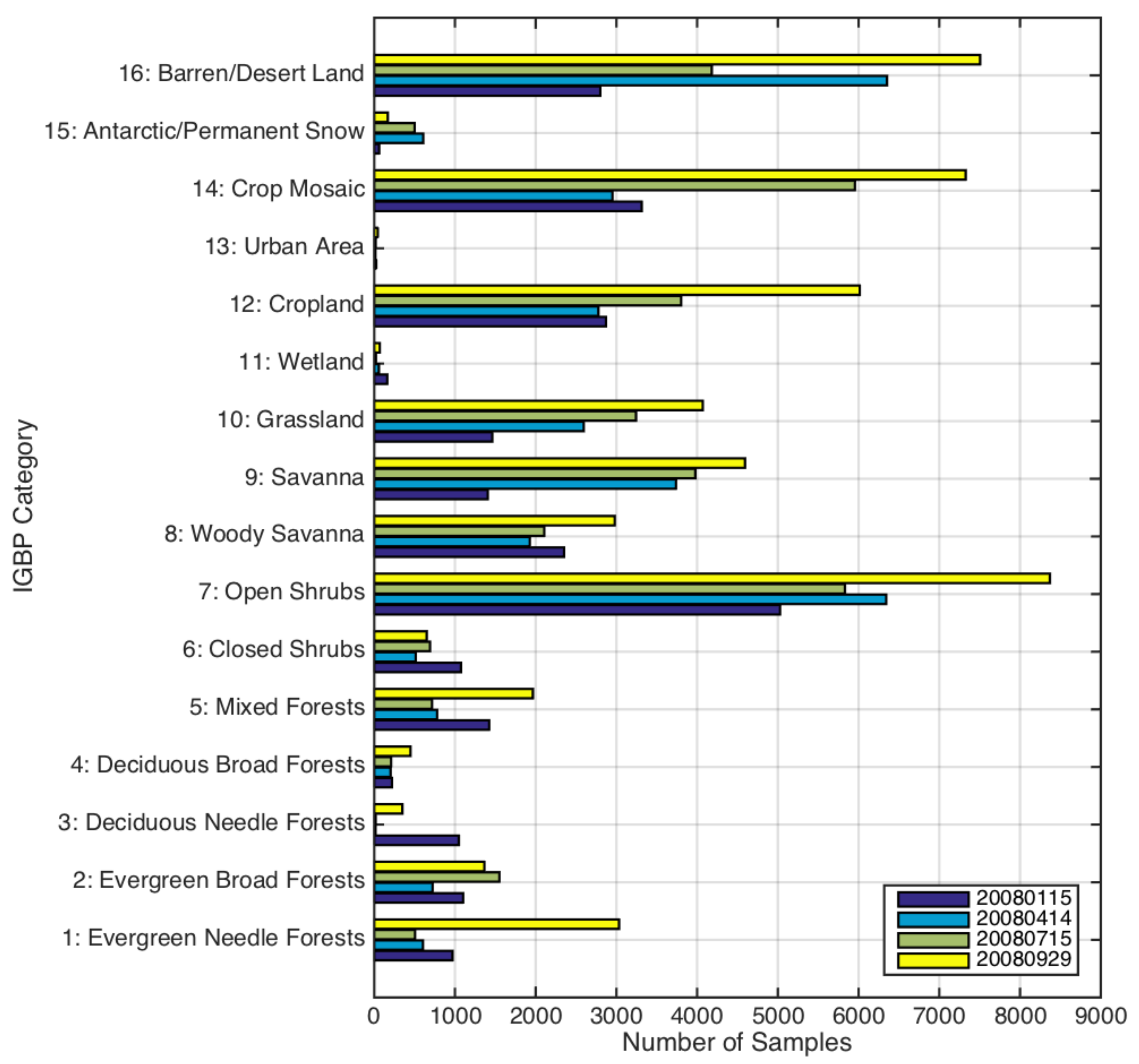
Figure 10.
Number of samples for de-biased variances listed in Table 4.
Figure 10.
Number of samples for de-biased variances listed in Table 4.


Table 1.
Bands, inputs, and methodology for generating the CAMEL (Combined ASTER and MODIS Emissivity over Land, combining the Moderate Resolution Imaging Spectroradiometer (MODIS) and the Advanced Spaceborne Thermal Emission and Reflection Radiometer (ASTER)) product and algorithm uncertainty estimates *. Note University of Wisconsin Baseline-Fit (UW BF) is based on the MODIS emissivity product.
| CAMEL Channel Number | CAMEL Wavelength [μm] | UWBF | ASTER | CAMEL COMBINING METHOD | ALGORITHM UNCERTAINTY |
|---|---|---|---|---|---|
| 1 | 3.6 | Y | - | UWBF1 | Abs(UWBF1 × [(UWBF6 − ASTER2)/UWBF6])/√3 |
| 2 | 4.3 | Y | - | UWBF2 | Abs(UWBF2 × [(UWBF6 − ASTER2)/UWBF6])/√3 |
| 3 | 5.0 | Y | - | UWBF3 | Abs(0.01)/√3 |
| 4 | 5.8 | Y | - | UWBF4 | Abs(0.01)/√3 |
| 5 | 7.6 | Y | - | UWBF5 | 0 (Minimal variation) |
| 6 | 8.3 | Y | Y | ASTER 1 + (CAMEL7(UWBF6, ASTER 2) − ASTER 2) | Abs(UWBF6 − ASTER1)/√3 |
| 7 | 8.6 | Y | Y | Weighted Mean(UWBF6, ASTER 2) | Abs(UWBF6 − ASTER2)/√3 |
| 8 | 9.1 | - | Y | ASTER 3 + (CAMEL7(UWBF6, ASTER 2) − ASTER 2) | Abs(UWBF6 − ASTER3)/√3 |
| 9 | 10.6 | - | Y | ASTER 4 | Abs(UWBF8 − ASTER4)/√3 |
| 10 | 10.8 | - | - | Linear Interpolation(ASTER 4, ASTER 5) | Abs(UWBF8 − [(ASTER4 × 5 + ASTER5 × 2)/7])/√3 |
| 11 | 11.3 | - | Y | ASTER5 | Abs(UWBF8 − ASTER5)/√3 |
| 12 | 12.1 | Y | - | UWBF9 but if ASTER5 > UWBF9, UWBF9 + diff(UWBF9, ASTER 5) × w | Abs(UWBF9 − ASTER5)/√3 |
| 12 * | 12.1 | Y | - | if snowfrac > 0.5UWBF9 + diff(CAMEL10, UWBF8) | Abs(UWBF9 − ASTER5)/√3 |
| 13 | 14.3 | Y | - | UWBF10 but if ASTER 5 > UWBF9, UWBF9 + diff(UWBF9, ASTER 5) × w | Abs(UWBF10 − ASTER5)/√3 |
| 13 * | 14.3 | Y | - | if snowfrac > 0.5, CAMEL12 | Abs(UWBF10 − ASTER5)/√3 |
* For more details on the CAMEL Combining Method, see Part 1 of this paper series. In the table w represents a weight factor. CAMEL channels 12 and 13 have separate combing methods based on whether the pixel is defined as snow or non-snow.
Table 2.
Definition of CAMEL emissivity uncertainty quality flag.
| Value | Description |
|---|---|
| 0 | Ocean or no CAMEL data available |
| 1 | Good quality |
| 2 | Unphysical uncertainty |
Table 3.
Definition of CAMEL quality flag.
| Value | Description |
|---|---|
| 0 | Ocean or inland water |
| 1 | input UW BF and ASTER data are good quality |
| 2 | input UW BF is good quality and ASTER is filled |
| 3 | the input UW BF is filled but ASTER is good quality |
| 4 | both the UW and ASTER values are filled |
Table 4.
Variance over the 8–9 µm region of de-biased IASI calculated minus observed BTs are averaged by IGBP land classification categories for four focus days and shown below in units of Kelvin for nighttime cases. De-biased variances for BTs calculated using a constant 0.98 emissivity and the CAMEL HSR emissivity module are shown. The corresponding number of samples are shown in Figure 10.
| IGBP Category | 15 January 2008 | 14 April 2008 | 15 July 2008 | 29 September 2008 | ||||
|---|---|---|---|---|---|---|---|---|
| 0.98 | CAMEL | 0.98 | CAMEL | 0.98 | CAMEL | 0.98 | CAMEL | |
| 1: Evergreen Needle Forests | 3.48 | 3.48 | 1.35 | 1.45 | 3.48 | 3.38 | 2.89 | 2.86 |
| 2: Evergreen Broad Forests | 5.21 | 4.95 | 5.76 | 5.49 | 6.19 | 5.81 | 2.33 | 2.14 |
| 3: Deciduous Needle Forests | 1.98 | 1.98 | 5.99 | 6.02 | 7.91 | 7.49 | 1.31 | 1.29 |
| 4: Deciduous Broad Forests | 2.22 | 2.23 | 1.92 | 2.06 | 3.03 | 2.84 | 4.37 | 4.44 |
| 5: Mixed Forests | 1.97 | 1.96 | 1.24 | 1.3 | 5.34 | 4.96 | 2.73 | 2.64 |
| 6: Closed Shrubs | 2.27 | 1.98 | 3.61 | 3.57 | 3.62 | 3.2 | 2.87 | 2.41 |
| 7: Open Shrubs | 4.8 | 2.57 | 4.16 | 1.48 | 4.83 | 1.89 | 4.31 | 1.62 |
| 8: Woody Savanna | 3.01 | 2.88 | 3.92 | 3.59 | 4.67 | 4.21 | 3.08 | 2.67 |
| 9: Savanna | 3.76 | 2.93 | 3.77 | 3.11 | 4.68 | 3.75 | 2.18 | 1.52 |
| 10: Grassland | 2.85 | 2.34 | 2.9 | 2.17 | 2.56 | 1.92 | 2.26 | 1.63 |
| 11: Wetland | 1.83 | 1.84 | 1.24 | 1.3 | 3.63 | 3.4 | 2 | 1.78 |
| 12: Cropland | 2.71 | 2.51 | 2.19 | 1.81 | 3.47 | 3.12 | 2.84 | 2.61 |
| 13: Urban Area | 2.67 | 2.68 | 1.77 | 1.9 | 4.39 | 4.22 | 3.78 | 3.71 |
| 14: Crop Mosaic | 3.34 | 3.15 | 2.62 | 2.45 | 3.9 | 3.55 | 3.1 | 2.75 |
| 15: Antarctic/Permanent Snow | 1.25 | 1.3 | 1.16 | 1.2 | 1.46 | 1.45 | 1.57 | 1.72 |
| 16: Barren/Desert | 6.96 | 2.28 | 13.4 | 2.16 | 10.3 | 2.62 | 14.2 | 1.85 |
© 2018 by the authors. Licensee MDPI, Basel, Switzerland. This article is an open access article distributed under the terms and conditions of the Creative Commons Attribution (CC BY) license (http://creativecommons.org/licenses/by/4.0/).
Share and Cite
MDPI and ACS Style
Feltz, M.; Borbas, E.; Knuteson, R.; Hulley, G.; Hook, S. The Combined ASTER MODIS Emissivity over Land (CAMEL) Part 2: Uncertainty and Validation. Remote Sens. 2018, 10, 664. https://0-doi-org.brum.beds.ac.uk/10.3390/rs10050664
AMA Style
Feltz M, Borbas E, Knuteson R, Hulley G, Hook S. The Combined ASTER MODIS Emissivity over Land (CAMEL) Part 2: Uncertainty and Validation. Remote Sensing. 2018; 10(5):664. https://0-doi-org.brum.beds.ac.uk/10.3390/rs10050664
Chicago/Turabian StyleFeltz, Michelle, Eva Borbas, Robert Knuteson, Glynn Hulley, and Simon Hook. 2018. "The Combined ASTER MODIS Emissivity over Land (CAMEL) Part 2: Uncertainty and Validation" Remote Sensing 10, no. 5: 664. https://0-doi-org.brum.beds.ac.uk/10.3390/rs10050664
Note that from the first issue of 2016, this journal uses article numbers instead of page numbers. See further details here.