Optimal Seamline Detection for Orthoimage Mosaicking Based on DSM and Improved JPS Algorithm


1
College of Marine Science and Technology, China University of Geosciences, Wuhan 430074, Hubei, China
2
Faculty of Information Engineering, China University of Geosciences, Wuhan 430074, Hubei, China
3
Faculty of Computer sciences, China University of Geosciences, Wuhan 430074, Hubei, China
*
Author to whom correspondence should be addressed.
Remote Sens. 2018, 10(6), 821; https://0-doi-org.brum.beds.ac.uk/10.3390/rs10060821
Submission received: 10 April 2018
/
Revised: 5 May 2018
/
Accepted: 17 May 2018
/
Published: 25 May 2018
(This article belongs to the Special Issue Instrumenting Smart City Applications with Big Sensing and Earth Observatory Data: Tools, Methods and Techniques)
Abstract
:Based on the digital surface model (DSM) and jump point search (JPS) algorithm, this study proposed a novel approach to detect the optimal seamline for orthoimage mosaicking. By threshold segmentation, DSM was first identified as ground regions and obstacle regions (e.g., buildings, trees, and cars). Then, the mathematical morphology method was used to make the edge of obstacles more prominent. Subsequently, the processed DSM was considered as a uniform-cost grid map, and the JPS algorithm was improved and employed to search for key jump points in the map. Meanwhile, the jump points would be evaluated according to an optimized function, finally generating a minimum cost path as the optimal seamline. Furthermore, the search strategy was modified to avoid search failure when the search map was completely blocked by obstacles in the search direction. Comparison of the proposed method and the Dijkstra’s algorithm was carried out based on two groups of image data with different characteristics. Results showed the following: (1) the proposed method could detect better seamlines near the centerlines of the overlap regions, crossing far fewer ground objects; (2) the efficiency and resource consumption were greatly improved since the improved JPS algorithm skips many image pixels without them being explicitly evaluated. In general, based on DSM, the proposed method combining threshold segmentation, mathematical morphology, and improved JPS algorithms was helpful for detecting the optimal seamline for orthoimage mosaicking.
1. Introduction
Image mosaicking is an essential step in production of large-scale digital orthophoto maps (DOM). At present, human intervention is still needed during the production to prevent the seamline from passing through obvious ground objects such as buildings, trees, and cars, which may cause dislocations and fractures to final mosaic DOM [1,2,3,4]. Therefore, how to detect an optimal seamline while avoiding obvious ground objects, to obtain a high-quality orthoimage, has become one of the research hotspots in the field of computer vision, photogrammetry, and remote sensing [2,4,5,6,7,8].
The process of seamline detection can be divided into two major steps: (1) generating a map composed of obstacle and non-obstacle regions (or a continuous weighted map) for seamline detection; (2) using different techniques to determine the seamline in generated map. Traditional methods [2,5,8,9,10,11,12,13,14,15] used the per-pixel-based gray information (e.g., grayscale and gradient difference, image edge, color, and texture information) of DOM pair’s overlap to generate a cost map, and then different path planning algorithms such as Dijkstra’s algorithm [16], snake model [5], A* algorithm [17], graph cuts [18] and dynamic programming algorithm [19] were applied to determine a minimum cost path as the final seamline. For example, the Dijkstra’s algorithm was first used to detect the seamline in difference images of DOM pairs for mosaicking by Davis [9], while the algorithm complexity would be too high. Kerschner [5] proposed a twin-snake model to detect an optimal path with the lowest difference in combination of grayscale, colors, and textures as the seamline. However, the iterative search was easy to stop at the minimum of the local energy and the algorithm might only have good results for forest areas. Zhang et al. [10] used ant colony algorithms for seamline extraction, which could avoid crossing obstacles and regions with large color contrast, but it was sensitive to the number of ants and might tend to get local optimal solutions. Chon et al. [11] added the minimizing of the local mismatch algorithm to optimize the Dijkstra’s algorithm. The method could effectively suppress the local maximum gray scale with a minimal objective function, and a better seamline was detected. Yu et al. [2] combined image similarity constraints (including information of color, edge, and texture), image saliency and location constraints to generate a total cost image, and then determined the optimal seamline with a dynamic programming algorithm.
The seamline extracted by the abovementioned methods based on gray difference information of the overlap could roughly avoid obstacles, which might be attributed to the fact that that information could only reflect the approximate ranges of the obstacles, and those ranges were usually non-continuous. The whole information of ground objects would be positive for optimal seamline detection. As a result, some researchers utilized DOM pairs to obtain object-based information of ground obstacles for detecting the seamline. For example, Pan et al. [4] presented a method based on the parallax map with semi-global matching (SGM) algorithm to obtain obstacle regions. Then, the skeleton line was generated, and the Dijkstra’s algorithm was applied to search for the seamline in the skeleton network. A similar method was proposed by Yuan et al. [20], while the greedy snake algorithm [21] was used to generate a seamline in processed parallax image. Li et al. [22] attempted to use the deep convolutional neural network (CNN) to classify the overlap region of the DOM pair into surface objects and assigned weights to each pixel according to the classification probabilities. Then, graph cuts algorithm was used to find the optimal seamline. The algorithm was effective, while the training sample was needed, and the algorithm might take a long time. Dong et al. [23] developed a method based on a parametric kernel graph cuts segmentation algorithm with a global cost map to avoid the seamline crossing obvious objects. Some other researchers used extra data to obtain obstacles in the search map, such as digital surface model (DSM) data [3,21,24,25], light detection and ranging (LiDAR) point cloud [26], vector building maps [27], and vector road data [28,29]. Meanwhile, different algorithms were used to determine the final seamline in the search map.
For recognizing obstacle regions, those researches based on object-based information maps derived from original DOM needed a more complex calculation process, making it difficult for practical DOM production. Those with extra data could obtain high-quality seamlines with a lower consumption of time and resources. As for a seamline search strategy, most existing algorithms chose to search the seamline pixel by pixel in the search map. The search efficiency should be furthermore improved. As a result, this study presented a novel seamline detection approach based on DSM and an improved jump point search (JPS) algorithm.
The JPS algorithm [30,31] is an online path-finding algorithm based on uniform-cost grid map, which is usually used to optimize the A* algorithm. The algorithm is efficient and has been applied to many path-finding fields such as robotics and games, while it has not been examined in the field of image mosaicking. The standard JPS algorithm was improved in this study to overcome its limitations and make it more effective for optimal seamline detection. The evaluation function was optimized with central constraint to make the seamline near the centerline of image pair’s overlap region. Moreover, the search strategy of the JPS algorithm was modified to avoid search failure when the search map was completely blocked by obstacles in the search direction. The main steps of the method were as follows: first, the overlap of DSM was processed and divided into obstacle regions and non-obstacle regions. Second, the mathematical morphology method was used to make the obstacles more prominent, generating a uniform-cost grid map. Then, improved JPS algorithm was applied to search for the jump points in the map and ignore other pixels that did not need to be explicitly considered. Meanwhile, an evaluation function was defined to estimate the moving cost of each jump point. Finally, an optimal path would be generated as the final seamline after evaluating those jump points. Comparison of the proposed method and the Dijkstra’s algorithm was carried out based on two groups of image data with different characteristics.
2. Methods
The proposed method was mainly divided into two major parts: (1) generation of obstacle regions; (2) seamline detection based on improved JPS algorithm. Those two parts are described further in the next two sections (Section 2.1 and Section 2.2).
2.1. Generation of Obstacle Areas
2.1.1. Selection of the Search Map
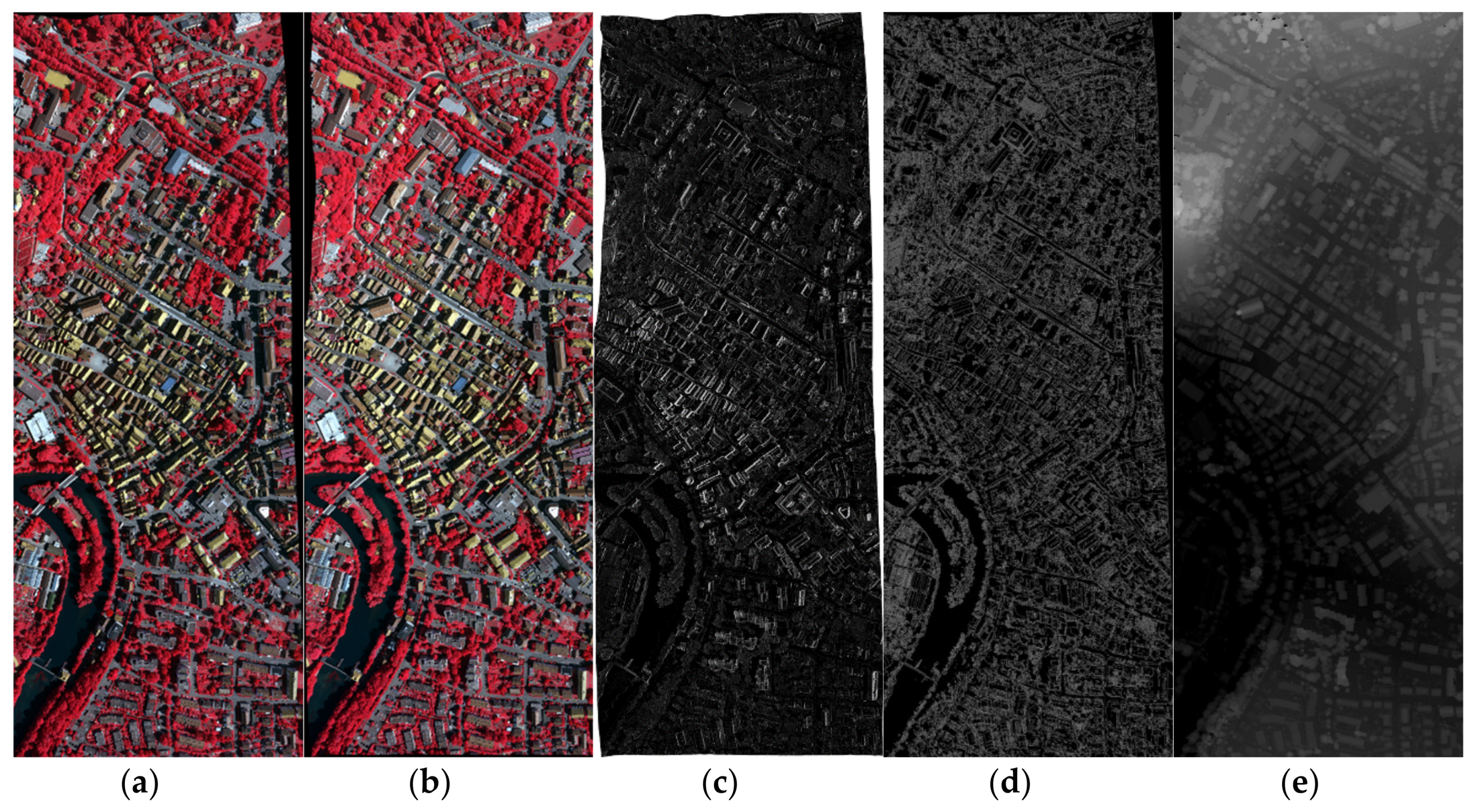
The essence of the seamline extraction is to find an optimal path avoiding crossing obstacle regions in the search map [20]. In many existing methods, difference image of DOM pair was used directly or indirectly to obtain obstacle regions in the search map. As shown in Figure 1a,b, DOM pair was obtained based on digital elevation model by digital differential rectification. Projection differences still existed in those areas above the ground such as buildings, trees, and cars. As a consequence, the edge of these regions was usually shown as the region with large gray value in the greyscale difference image (Figure 1c). It could be seen in Figure 1c that the edge of obstacles was non-continuous, and the gray value of the roof was usually small, leading to the seamline passing through the buildings. The characteristics in Figure 1c might be similar to other feature maps directly obtained from original DOM such as edge image (Figure 1d). Figure 1e was a grayscale map of original DSM. Compared to the difference image, it directly reflected the height and range information of ground objects, which could be used to make the seamline avoid crossing those areas. Therefore, the DSM was chosen as the search map.
2.1.2. Threshold Segmentation Operation
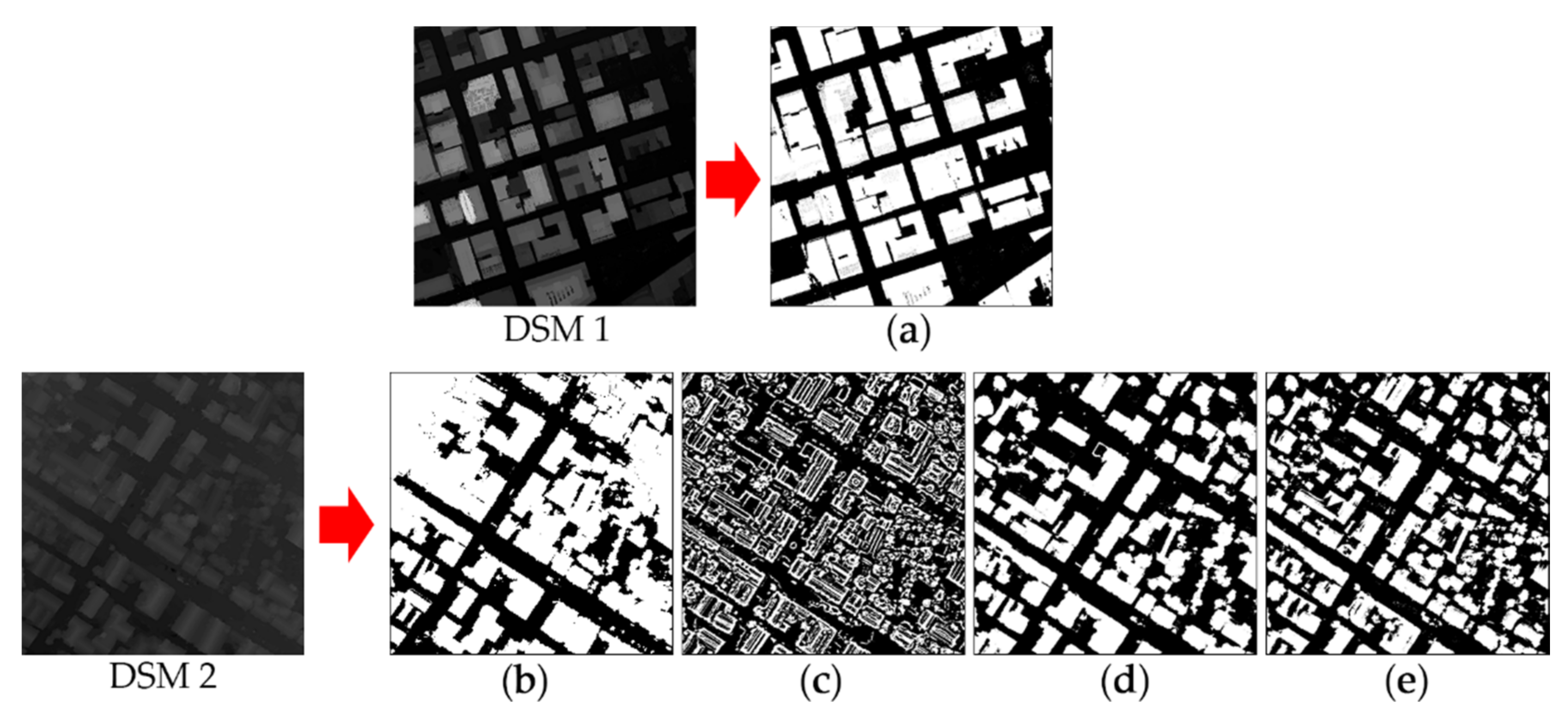
Threshold segmentation method was used to divide the DSM grayscale map of the image pair’s overlap into obstacle regions and non-obstacle regions. If the topography of the survey region was relatively flat, the image could be directly segmented according to a global threshold, as shown in Figure 2a. However, in some regions with large terrain variation, the gray value of the ground region in DSM grayscale map was quite different. As a result, the segmentation result might be poor with using the global threshold, as shown in Figure 2b. Therefore, local adaptive threshold segmentation method [32] was used to produce a binary image with better quality. The grey value of each pixel could be calculated by
where is the calculated grey value of the pixel in row r and col c; is the source grey value of the pixel in row r and col c; The threshold value is the mean of the neighborhood of the pixel in row r and col c minus an adjustment constant C.
Usually, an adjustment was not needed, and the value C could be set to zero. The blocksize N could be determined by experience or a trial-and-error process to produce a better segmentation image. Generally, when the value N was set smaller, some details could be preserved while there might be holes in obstacle regions (shown in Figure 2c). On the other hand, when the value was set larger, particularly obvious obstacles could be accurately detected while some details may be lost (shown in Figure 2d), and a longer calculation time was needed. As a result, the strategy in this study was to choose a smaller value as well as to ensure that obvious non-ground objects could be effectively segmented with smallest possible holes in obstacles (Those holes could be filled after being processed with morphological opening operation (described in Section 2.1.3)). An example can be seen in Figure 2e with N = 85 and C = 0 (two values were used in both experiments in this study).
2.1.3. Morphological Opening Operation
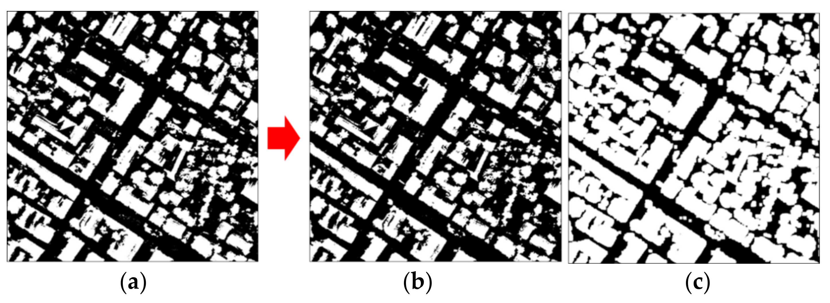
If the seamline was searched directly in the binary segmented map of DSM, it might be full of twists and turns because of noise pixels in segmentation image. Furthermore, the outlines of obstacles in DSM and DOM were not completely match due to different projection types. As a result, when the seamline was too close to the edges of the obstacle regions in the DSM, it might have crossed the edge of those regions in the DOM. Therefore, the DSM segmentation image was processed with morphological opening operation [32]. First, the image was eroded with a small convolution kernel to eliminate grayscale changes caused by small noise pixel areas, then dilated with a large convolution kernel to fill the holes of obstacle regions and make the edges of obstacles extend out. As a result, the final seamline could deviate from buildings, cars or trees in the mosaic image. Figure 3a,b showed the results of morphology opening operation.
2.2. Seamline Detection Based on an Improved JPS Algorithm
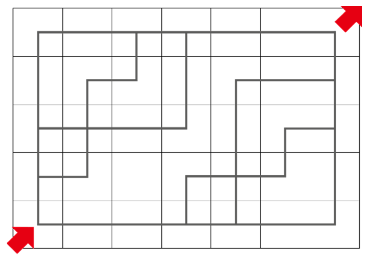
The JPS algorithm was first proposed by Daniel Harabor and Alban Grastien [30,31] to find path on uniform-cost grid map, which can speed up A* algorithm by an order of magnitude [30]. The thought of the algorithm is to follow some rules (for details see Section 2.2.1) to jump over many pixels that do not need to be explicitly considered in the grid map. As a result, the path symmetry (an illustration can be shown in Figure 4) is broken, avoiding unnecessary symmetric path search process and greatly improving the search efficiency [30,31,33].
In this study, the processed binary image of DSM was considered as an 8-connected grid map. Each pixel in the processed DSM corresponded to a grid node in the grid map. When the start and finish point of the seamline were determined, the JPS algorithm was used to find the jump points in the map. Meanwhile, the search cost of each jump point was evaluated to generate an optimal path as the final seamline with minimum cost.
2.2.1. The Principle of JPS Algorithm
The main steps of the JPS algorithm include: (1) recognizing and removing unrelated nodes in the grid map, also called node pruning; (2) searching for key jump points in the grid map. JPS algorithm works with the two following rules:
Node Pruning Rules: Define the cost of one straight move step as 1, one diagonal move step as . For the given node x reached via a parent node in the grid map, the node n () will be pruned from its neighbor node set if one of the following three principles is satisfied:
- (1)
- There is a path from node to node n, that is strictly shorter than the path from node to node n via node x.
- (2)
- There is a path from node to node n via node y, that is strictly shorter than the path from node to node n via node x.
- (3)
- There is a path from node to node n via node y, with the same length as the path from node to node n via node x, but path moves earlier than path with a diagonal type.
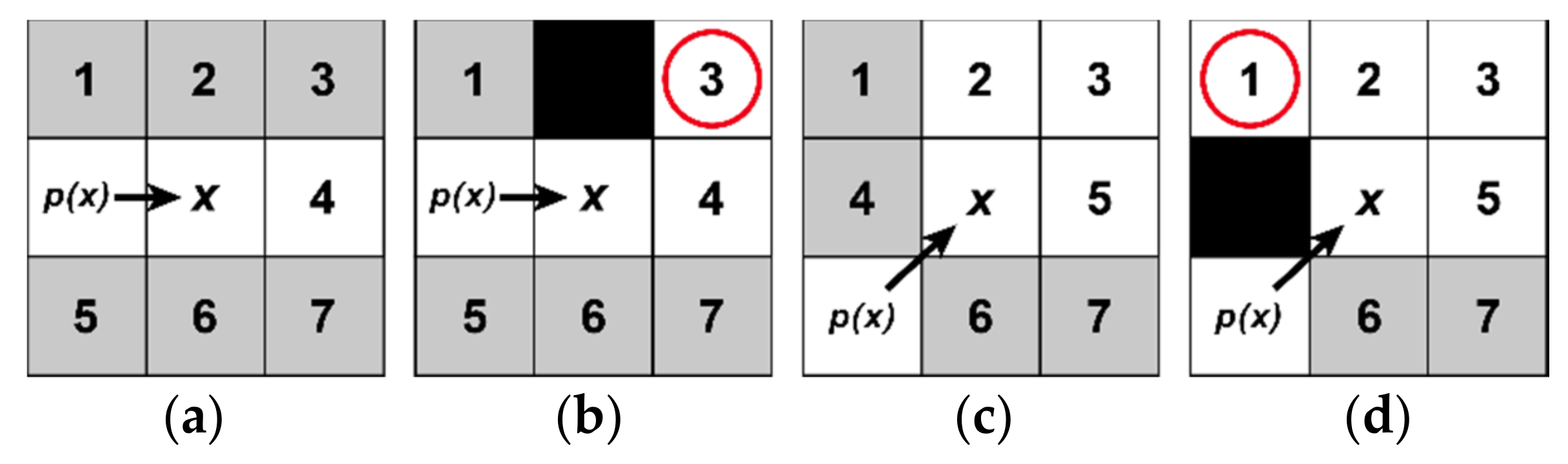
Figure 5 shows the examples of node pruning, those nodes marked with grey color will be pruned. In Figure 5a, the node 1, 2, 5, and 6 are pruned due to rule (1), the node 3 and 7 are pruned due to rule (3). In Figure 5c, the node 4 and 6 are pruned due to rule (1), the node 1 and 7 are pruned due to rule (2). As a result, only those nodes marked with white need to be considered, which are called the natural successors of the node x. Furthermore, as shown in Figure 5b,d, when contains obstacles, a small set of up to k (0 ≤ k ≤ 2) additional nodes (marked with red circle in in Figure 5b,d) is needed to be considered, these nodes are called forced neighbors of the current node x.
Jumping Rules: When JPS algorithm performs search process, the node pruning rule is followed recursively to prune the set of neighbors around each node, replacing each neighbor node n with a so-called jump point successor and skipping all unvisited nodes in the grid map. The recursion will stop when encountering an obstacle or a jump point is found in the search. Jump points have neighbors that cannot be reached by an alternative symmetric path and the optimal path must go through this jump point. The recursion search process of a jump point is described as follows:
- (1)
- Straight moves: from the start node x, respectively move to different neighbor nodes according to the straight natural successor directions, the node :
- (a)
- If node has forced neighbors, return node as a jump point successor of the node x;
- (b)
- If node is an obstacle or out of the map, just ignore this direction;
- (c)
- If nothing happens, repeat the above search process from the node .
- (2)
- Diagonal moves: from the start node x, respectively move to different neighbor nodes according to the diagonal natural successor directions, the node :
- (a)
- If node has forced neighbors, return node as a jump point successor of the node x;
- (b)
- If node is an obstacle or out of the map, just ignore this direction;
- (c)
- Implementing straight moves from the node , if there is a jump point successor of the node n, then return the node n as a jump point successor of the node x;
- (d)
- If nothing happens, repeat the above search process from the node .
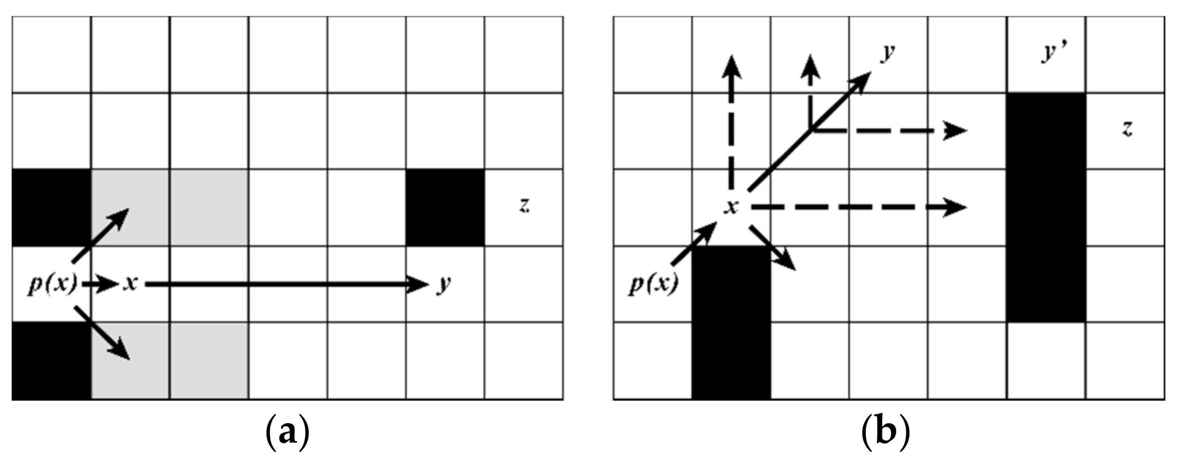
As shown in Figure 6a, move to the node x from its parent node p(x) and recursively apply the straight node pruning rules to prune the nodes in the grid map until the node y is found. Since the node y has a forced neighbor z, the node y is marked as a jump point successor of the node x. In Figure 6b, Since the node y has a jump point successor (with a forced neighbor z), the node y is returned as a jump point.
According to node pruning rules and jumping rules, those nodes that do not need to be accessed in the grid map can be pruned and only some jump points will be considered in the search algorithm. Notice that the process of node pruning is performed entirely online, the algorithm includes no preprocessing operation and has no memory overhead [30].
2.2.2. Optimal Seamline Detection
When mosaicking orthoimage in practical production, the initial seamline network could be generated by the method of the area Voronoi diagram with overlap [6,34]. Then, the seamline was optimized according to the start and target point of polygon edges in seamline network. To avoid the case that the begin point and target point of the initial seamline were in the obstacle region, the points needed to be dynamically adjusted in actual search process. The specific method is: take the initial point O as the origin, increase the radius R gradually from zero, and randomly select the non-obstacle point in generated circle as the new start point or target point. In this study, , where width represents the width of the original image.
In seamline optimization process, when a jump point n was found in the processed map of DSM, the search cost of the node n was calculated by
where is an estimate of the minimum cost from start point to target point via the node n. represents the cost moving from point n to the target point, which can be calculated by Manhattan distance that moves only along the horizontal and vertical directions. represents the cost moving from start point to point n via different intermediate points. It can be calculated by a recursive function:
where is the parent node of the node n, means the moving cost from node to the node n.
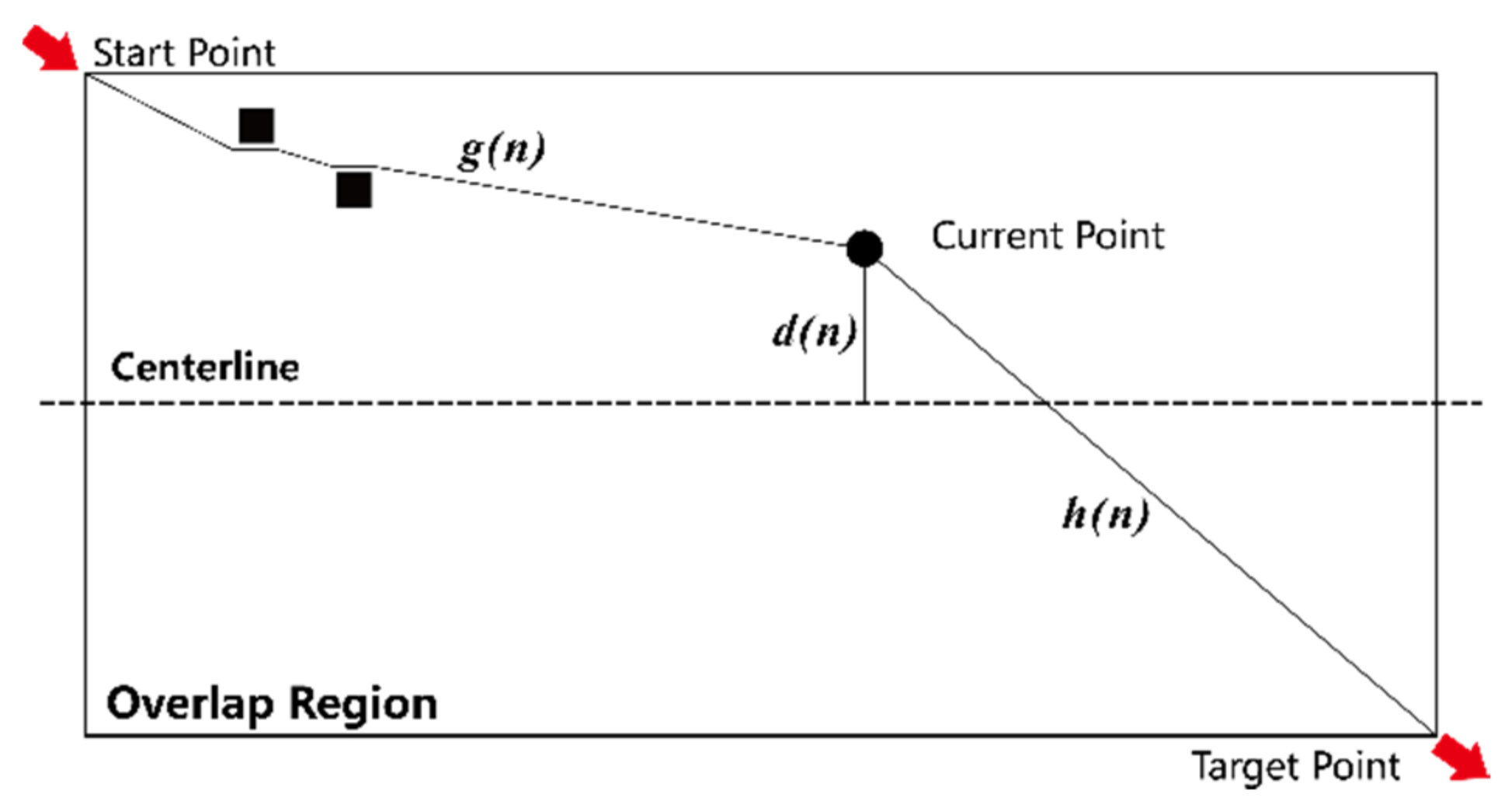
The aerial digital image is usually obtained with a pattern of central projection. In center of the projection, the image quality is higher due to the smaller geometric distortion, which is the same as DOM obtained after digital differential rectification [6,10]. Therefore, the optimal seamline should meet the principle that the seamline should be close to the centerline (initial seamline) of the image pair’s overlap region [2,10,20,26]. Thus, the evaluation function was optimized with a central constraint to make the seamline closer to centerline of the overlap. The search cost of the node n would become higher when the distance from node n to the centerline increased. The function after optimization was defined as
where d is the distance from node n to the centerline of the image, as shown in Figure 7, is the maximum allowable distance offset from centerline of the overlap area, and is an influence factor. In general, the factor could be set to a value ranging from 0.5 to 1, ensuring optimized function had an appropriate influence on the final seamline. In this study, .
In actual search process, the open list and the close list were set up to store the unprocessed and processed nodes respectively. The steps of searching for the seamline with improved JPS algorithm were as follows:
- (1)
- Add the start node to the open list, set the close list to empty, and start search from start node to all neighbor nodes separately.
- (2)
- If there were nodes in the open list, select the node n with the lowest cost value . If node n was the target node, then the path search was completed, otherwise it would be removed from the open list and added to the close list, and no longer needed to be evaluated.
- (3)
- From the node n, search for the jump point t (node t) in the direction of its natural successors:
- (a)
- If there was no returned node or the returned node t was in the close list, just ignore it;
- (b)
- If the returned node t was not in the open list, add the node t to the open list and calculate its , and values. Regard the node n as the parent node of the node t and record the parent direction of the node t;
- (c)
- If node t was in the open list, calculate the new value to see whether it was lower than the previous . If so, change its parent to the node n and calculate its value.
- (4)
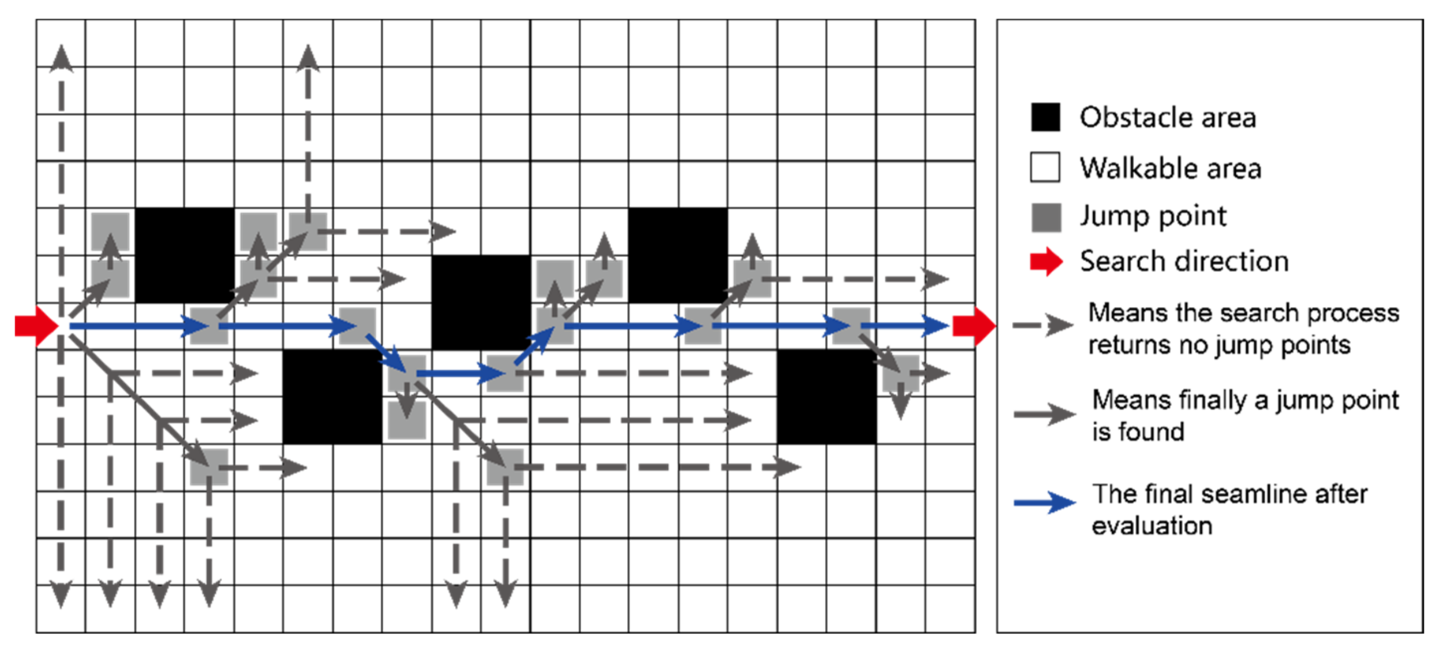
- Repeat the step (2) to step (3) until the target node was found, the optimal path was then generated according to the recorded parent direction. Figure 8 is an illustration of the path search process.
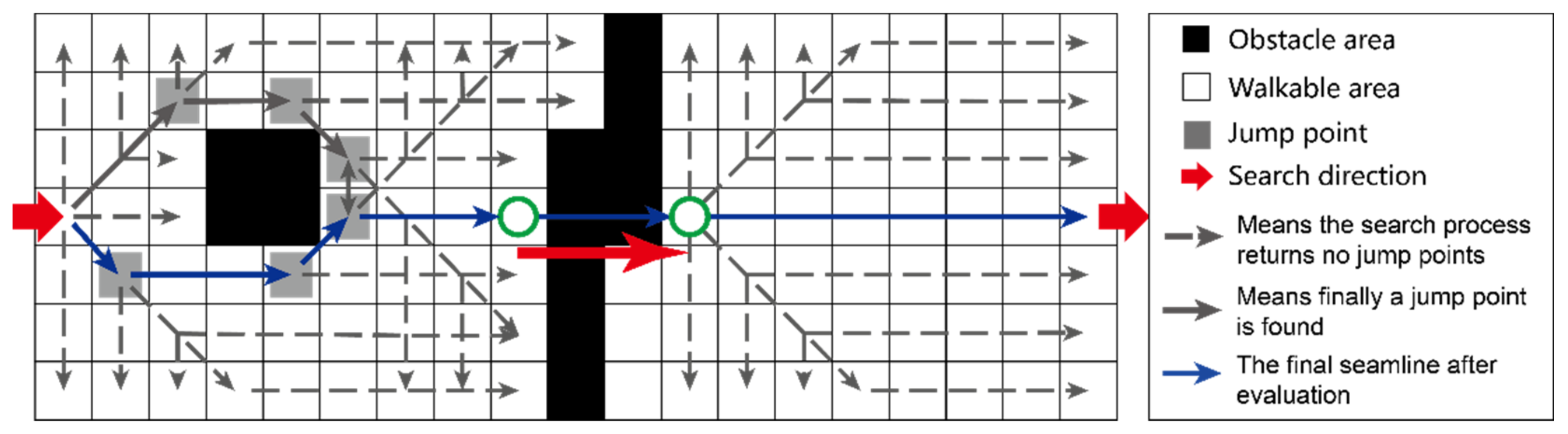
In some extreme cases, the processed DSM map might be completely segmented by obstacles in the search direction, which led to the failure of the seamline search. In actual search process, the path search would fail when the open list was empty due to that there were no jump points to be evaluated. The solution to this situation in this study was as follows: select the node n with the lowest value (meant the node n was closest to the target node) in the close list, and generate a path from start point to the node n according to the parent direction of each node; then cross obstacles from the node n in a straight line parallel to the overlap’s centerline; continue the search process with the first non-obstacle point as a new start point until the search was successful. Figure 9 is the illustration of the approach to this situation.
3. Experiment and Results
3.1. Design of Experiments
To verify the feasibility and validity of the proposed seamline detection method in this study, two groups of experiments with different DOM and DSM data were carried out. Area 1 was used for image pair mosaicking in experiment I, and area 2 was used for multi images (a strip containing 5 images) mosaicking in experiment II. The characteristics of two test areas are shown in Table 1. The original images were orthorectified and the DSM data of the overlap regions was obtained by SGM [4] algorithm. The comparative experiments involved the followings: (1) based on the difference images of DOM pairs and the Dijkstra’s algorithm [9], (2) based on processed DSM and the Dijkstra’s algorithm.
In general, the pixel resolution of aerial remote sensing images is too high. To avoid the consumption of irrelevant resources and improve the computing efficiency, the overlap regions of DSM and DOM were processed by down-sampling (bilinear interpolation [32]). After finishing the search, the node coordinates of the seamline needed be calculated to the original geographic coordinates of the DOM and DSM. All the algorithms in this study were implemented through C++ (VC14) programming with OpenCV (3.2.0). The test machine was a 2.60 GHz Intel Core i5-3230m Duo processor with 8 GB RAM running Windows 10.
3.2. Results
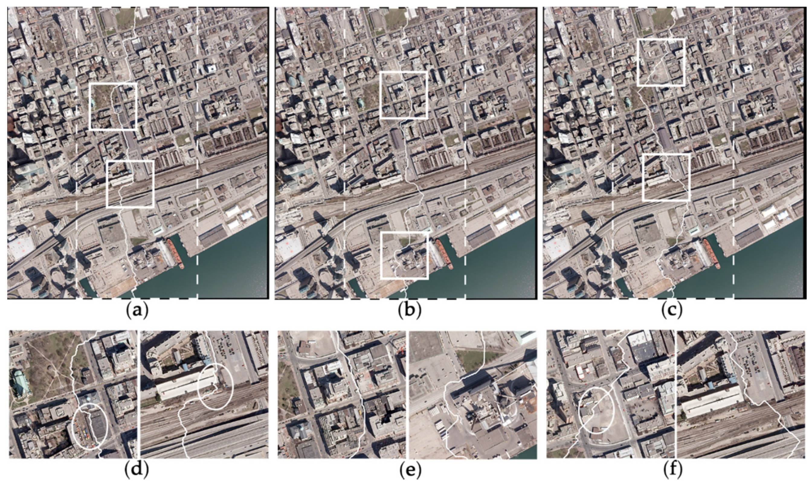
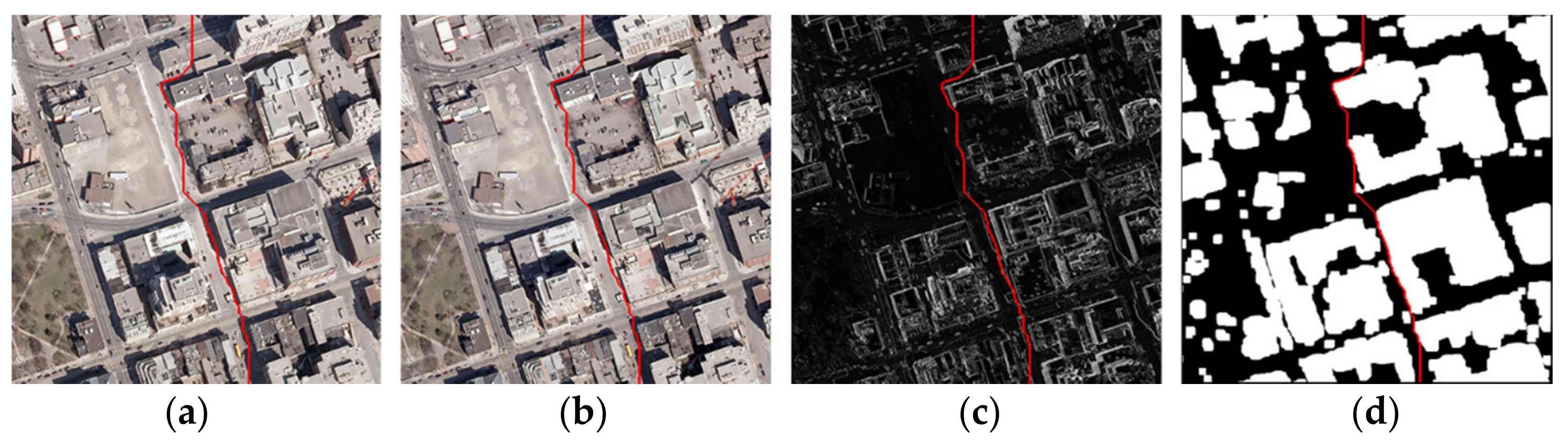
The results of experiment I were shown in Figure 10. Figure 10a shows the seamline extracted by the Dijkstra’s algorithm with difference image, which roughly avoided obvious obstacle regions. Since those obstacle regions were non-continuous in the difference image, it could be found that the seamline still crossed several buildings. Examples could be seen in white circles of Figure 10d. Figure 10b shows the seamline extracted by the proposed method. The extracted seamline was near the centerline of the image pair’s overlap region. Moreover, the seamline only crossed one building, and had a good avoidance effect on trees, vehicles, and other objects. Figure 10c shows the seamline extracted by the Dijkstra’s algorithm with processed DSM. The general effect was similar to the proposed method because the same search map was used, while the seamline crossed little more buildings and cars (as shown in white circles of Figure 10f). Reasons of crossing in those two methods with processed DSM might due to the too large projection difference or low segmentation quality at those places. Figure 11 shows the overlay of the seamline detected by the proposed algorithm on the subset of the original DOM pair, difference image, and processed DSM image, respectively. Obviously, the seamline did not cross any obstacles. In general, in the first experiment, the proposed method visually outperformed the other two.
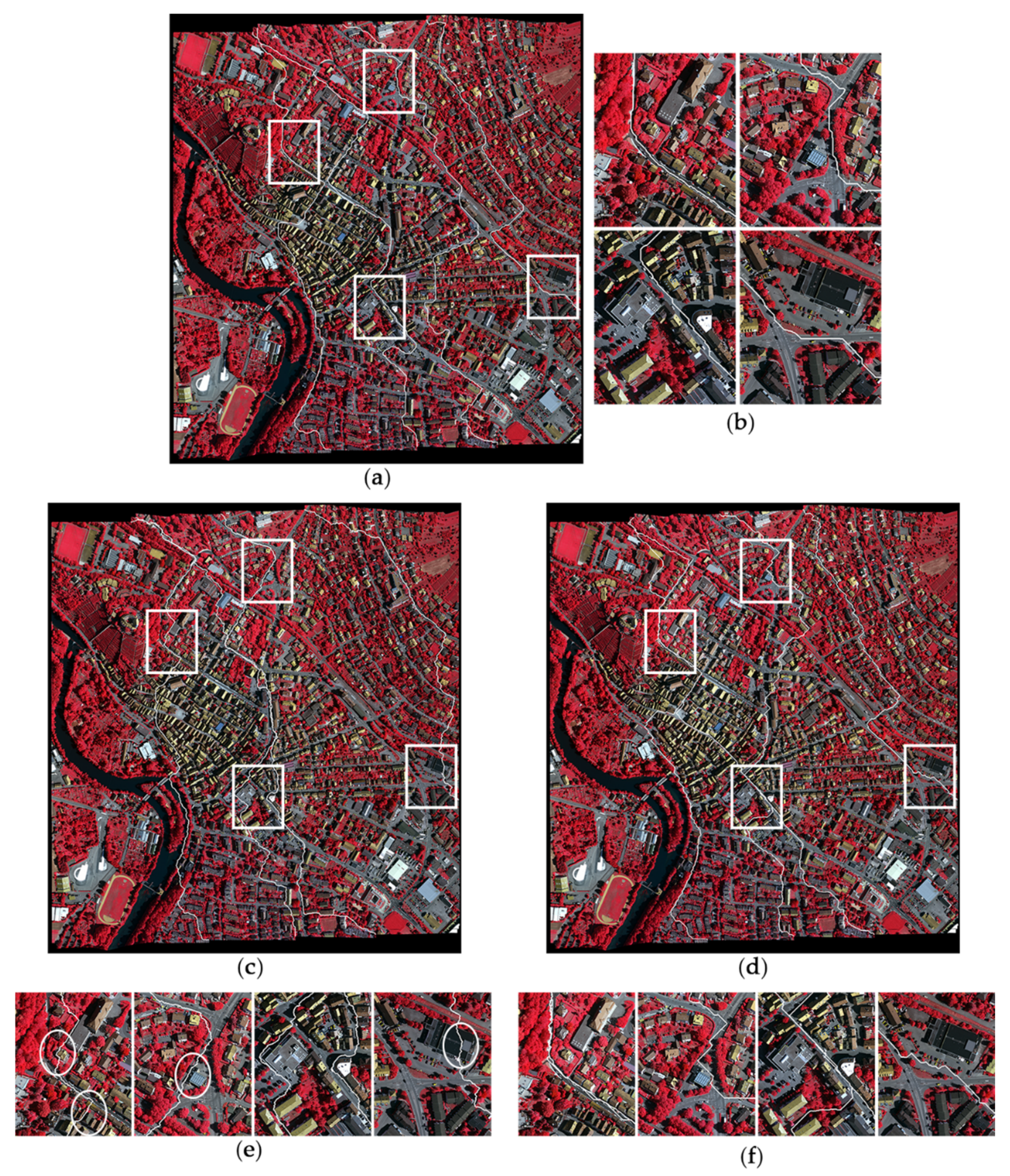
To further test and prove the effectiveness of the proposed method, a larger area containing 5 images was used for seamline extraction in experiment II, and results were shown in Figure 12. Figure 12a shows the seamline extracted by the proposed method, the overall effect was satisfactory with only crossing 2 buildings and several cars, and the extracted seamlines were evenly distributed without intersections in mosaic image. Figure 12c shows the seamline extracted by the Dijkstra’s algorithm with difference image, which had crossed much more obvious buildings. Examples can be seen in white circles of enlarged regions (Figure 12e). Furthermore, there were some intersections between different seamlines in the images. Figure 12d shows the seamline extracted by the Dijkstra’s algorithm with processed DSM. Compared with the proposed method, the effect was similar while the seamline crossed more buildings and cars, and phenomenon of seamlines intersections also occurred without a central constraint. Generally, the proposed method detected a better seamline in experiment II compared with other two methods.
Table 2 shows the statistical assessment metrics for those three seamline extraction algorithms in two groups of experiments. Obviously, the proposed algorithm had great advantages in terms of both efficiency (search time and total time) and resource consumption (memory usage) compared with those two Dijkstra’s algorithms. The process time of seamline detection and image mosaic greatly decreased with a low memory usage. In addition, the average gray level (G) values of the searched seamline nodes in difference image were calculated (Table 2). In theory, the better seamline is often with lower G value. The nodes in the seamline extracted by the proposed method were jump points, which always located at the edge of obstacle and non-obstacle area. As a result, the proposed method resulted in better seamlines with higher G values. What’ more, the numbers of obvious objects crossed by the seamline were obtained by artificial statistics. The proposed method crossed the least obvious ground objects than the Dijkstra’s method with difference image in both experiments. Notice that some low ground objects might not be accurately detected in the processed DSM, leading the seamline easily crossing those objects. As a result, the two DSM-based methods crossed a few more cars than the method with difference image.
The information of seamlines extracted in two experiments was counted. As shown in Table 3, the numbers of nodes in seamlines extracted by the proposed method were remarkably smaller than those by Dijkstra’s algorithm for both experiments, owing to that only jump points were considered as the seamline nodes. Furthermore, in the proposed method the percentages of evaluated nodes in all pixel nodes of the search map were less than one percent, while in the Dijkstra’s algorithm they were much larger. For example, for method 1 in experiment I, the proportion of evaluated nodes was up to ninety-nine percent, almost all the pixel nodes were evaluated. This can explain why the proposed method performed search so fast than the other two. Last, the average length of adjacent nodes and its variance in seamlines extracted by the proposed method were calculated. In experiment II the average length and variance was lower due to the buildings were smaller and surrounded trees were denser.
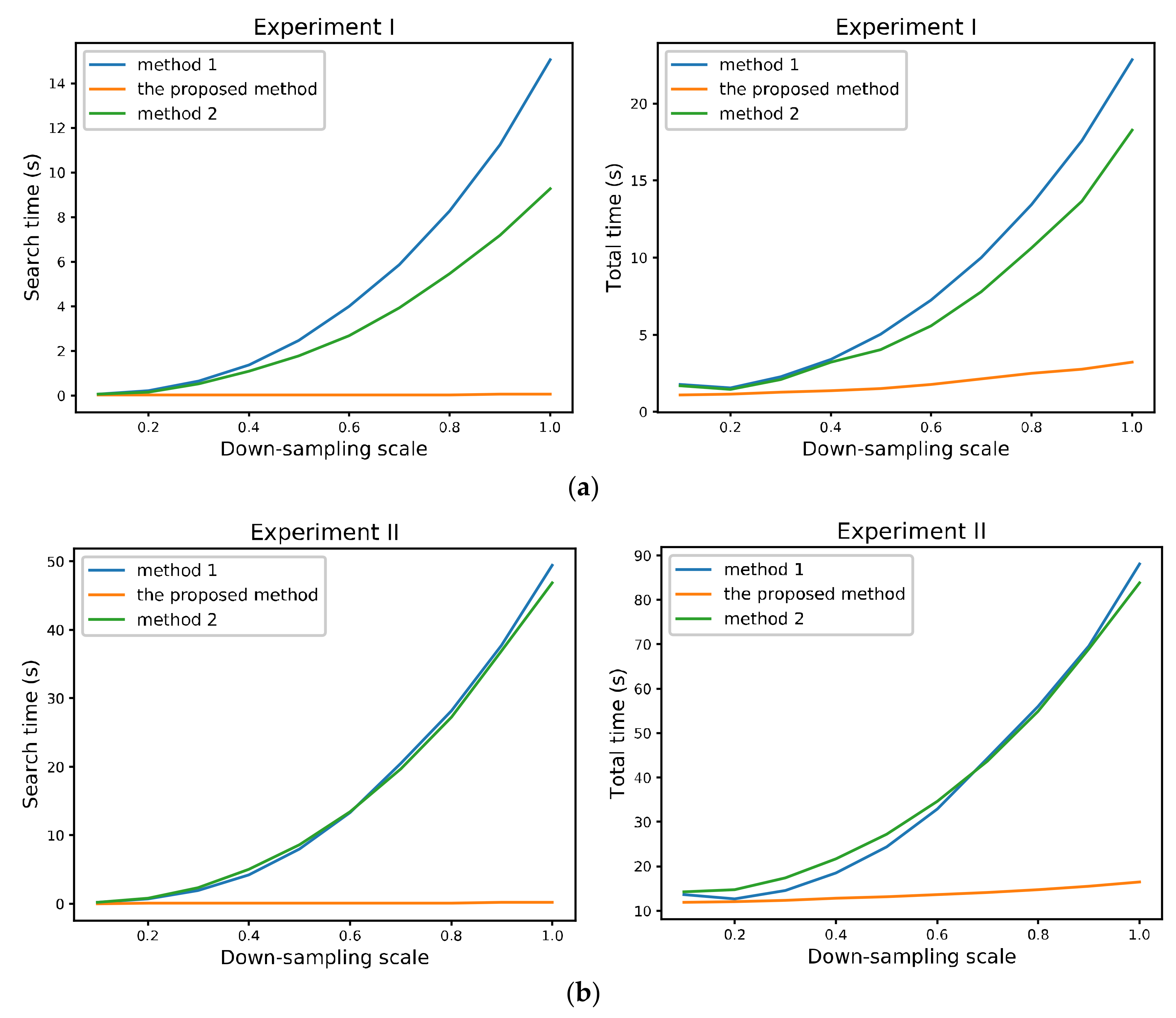
The search time of the above three seamline extraction methods under different pixel resolutions were also calculated. As shown in Figure 13, the search efficiency of the Dijkstra’s algorithm with difference image was close to that with processed DSM in the same experiment, and the gap depended on the difference of evaluated node percentages (shown in Table 3) in the search process. What’ more, when the image resolution increased, the time consumption of the Dijkstra’s algorithm was greatly increased, while the JPS algorithm did not increase much, due to that the number of jump points detected in new image did not increase a lot than before. In fact, the efficiency of JPS algorithm was also affected by the density of obstacles. The search process would accelerate if there were fewer obstacles in the map, because most pixels in the map were pruned and fewer jump points were detected. In general, with the increase of image resolution, the advantage of the proposed algorithm was more obvious.
4. Discussion
In this study, a novel seamline detection method based on improved JPS algorithm was proposed. The obtained results showed that the improved JPS algorithm was helpful for orthoimage mosaicking, and the seamline detected by the proposed method can effectively avoid passing through obvious objects on the ground with less resources consumption.
Many seamline detection methods were based on the grayscale difference information of the DOM pair’s overlap [2,5,8,9,10,11,12,13,14,15], and the resulting seamlines could roughly avoid obstacle regions. Since the obstacle regions were normally non-continuous in the final cost map (e.g., in the difference image or edge image the grey value of building edges is large while it is usually small for roofs), the seamline might still cross some obvious ground objects. As a result, this study was consistent with Chen et al. [3], Zuo et al. [21], and Zheng et al. [24,25], who chose to detect the seamline based on a DSM, because it directly reflects the height information and range of objects on the ground and helps to make the seamline avoid crossing these regions. Furthermore, in this study threshold segmentation and morphology operation were combined to process the DSM to make the seamline aloof from obstacles. Comparative experiments showed that the seamlines detected based on the DSM were better and more reliable than those based on the difference images.
In contrast to other researches based on a DSM, this study first used an improved JPS algorithm to search for the optimal seamline. The algorithm only considered the key jump points as the nodes of the final seamline and skipped other unrelated pixels rather than searching on a per-pixel basis, such as the Dijkstra’s algorithm [9], A* [26] or weighted A* [24]. Profiting from this, the search time and memory usage were greatly reduced in the proposed method. Meanwhile, the number of nodes in the seamline was much lower and the seamline was less circuitous, which were better for image mosaicking [35]. Furthermore, after optimizing the evaluation function with central constraint, the final seamlines were more likely to be near the centerlines of the image pair’s overlap areas. Although the seamlines extracted by the proposed method were better, due to the jump points always located at the edge of obstacle and non-obstacle area, the G values of the seamlines’ nodes derived from the proposed algorithm in the difference image were larger than those derived from the Dijkstra’s algorithm with difference image [9].
In the proposed method, the effect of seamline detection was closely related to the quality of original DSM and threshold segmentation result, because these two factors directly affected the final accuracy of the search map. Considering that the improved JPS algorithm could search for optimal seamline on the grid map composed of obstacle and non-obstacle regions, it might work well with the parallax image obtained by SGM algorithm [4], vector building maps [27] or the cost map classified by CNN [22], assuming that the calculation process with large resources consumption was acceptable in a real mosaicking process.
It should be noted that the study still had some limitations. First, the forcibly cross operation should be further optimized to make the seamline cross fewer obstacle pixels. In addition, when the flight height is too low, or the aerial area is filled with very high buildings, the projection difference of obstacles in final obtained DOM pairs will be too large. As a result, the detected seamline may be too close to the edge of these obstacles or even cross them. An orthoimage elevation synchronous model [3] may solve this problem while the additional digital terrain model data is needed. Lastly, the ground region was usually marked as a non-obstacle region, which might cause the seamline to pass through areas with large color differences on the ground. In the future, color and spectral information of ground objects will be added to optimize the seamline.
5. Conclusions
This study introduced a novel seamline detection approach based on DSM and an improved JPS algorithm. First, the DSM of the DOM pair’s overlap region was divided into the obstacle region and the non-obstacle region by combining threshold segmentation and morphological methods. Then, the improved JPS algorithm was used to prune unrelated pixels and detect jump points in the processed DSM. According to an optimized evaluation function, the cost of each jump point was estimated to obtain a minimum cost path as the final optimal seamline. Two groups of experiments by using improved JPS algorithm with processed DSM, and the Dijkstra’s algorithm based on difference image and processed DSM of DOM pair’ overlap, were carried out respectively. Results showed that the proposed JPS algorithm was effective and reliable for seamline detection, and the resulting seamlines could effectively avoid crossing obvious ground objects such as buildings, trees, etc. Since the JPS algorithm skipped a lot of pixel nodes that did not need to be evaluated, the quality of the finial seamline and image mosaic efficiency were greatly improved compared to the other two seamline extraction methods. In general, based on DSM and the proposed method combing threshold segmentation, mathematical morphology, and improved JPS algorithms was helpful for detecting the optimal seamline for orthoimage mosaicking.
Author Contributions
All authors made significant contributions to the manuscript. G.C. and S.C. conceived, designed and performed the experiments and wrote the manuscript together. X.L., P.Z. and Z.Z. helped to analyze the experiment results and revise the manuscript.
Acknowledgments
This research was jointly supported by the Fundamental Research Funds for the Natural Science Foundation of China (No. 41674015, 41274036). We acknowledge the International Society for Photogrammetry and Remote Sensing (ISPRS) for providing the public image dataset used in the study.
Conflicts of Interest
The authors declare no conflict of interest.
References
- Soille, P. Morphological image compositing. IEEE Trans. Pattern Anal. Mach. Intell. 2006, 28, 673–683. [Google Scholar] [CrossRef] [PubMed]
- Yu, L.; Holden, E.J.; Dentith, M.C.; Zhang, H. Towards the automatic selection of optimal seam line locations when merging optical remote-sensing images. Int. J. Remote Sens. 2012, 33, 1000–1014. [Google Scholar] [CrossRef]
- Chen, Q.; Sun, M.; Hu, X.; Zhang, Z. Automatic seamline network generation for urban orthophoto mosaicking with the use of a digital surface model. Remote Sens. 2014, 6, 12334–12359. [Google Scholar] [CrossRef]
- Pang, S.; Sun, M.; Hu, X.; Zhang, Z. SGM-based seamline determination for urban orthophoto mosaicking. ISPRS J. Photogramm. Remote Sens. 2016, 112, 1–12. [Google Scholar] [CrossRef]
- Kerschner, M. Seamline detection in colour orthoimage mosaicking by use of twin snakes. ISPRS J. Photogramm. Remote Sens. 2001, 56, 53–64. [Google Scholar] [CrossRef]
- Pan, J.; Wang, M.; Li, D.; Li, J. Automatic generation of seamline network using area Voronoi diagrams with overlap. IEEE Trans. Geosci. Remote Sens. 2009, 47, 1737–1744. [Google Scholar] [CrossRef]
- Pan, J.; Zhou, Q.; Wang, M. Seamline determination based on segmentation for urban image mosaicking. IEEE Geosci. Remote Sens. Lett. 2014, 11, 1335–1339. [Google Scholar] [CrossRef]
- Li, L.; Yao, J.; Lu, X.; Tu, J.; Shan, J. Optimal seamline detection for multiple image mosaicking via graph cuts. ISPRS J. Photogramm. Remote Sens. 2016, 113, 1–16. [Google Scholar] [CrossRef]
- Davis, J. Mosaics of scenes with moving objects. In Proceedings of the IEEE Computer Society Conference on Computer Vision and Pattern Recognition, Santa Barbara, CA, USA, 23–25 June 1998. [Google Scholar]
- Zhang, J.; Sun, M.; Zhang, Z. Automated seamline detection for orthophoto mosaicking based on ant colony algorithm. Geomat. Inf. Sci. Wuhan Univ. 2009, 34, 675–678. (In Chinese) [Google Scholar]
- Chon, J.; Kim, H.; Lin, C.S. Seam-line determination for image mosaicking: A technique minimizing the maximum local mismatch and the global cost. ISPRS J. Photogramm. Remote Sens. 2010, 65, 86–92. [Google Scholar] [CrossRef]
- Pan, J.; Wang, M. A seam-line optimized method based on difference image and gradient image. In Proceedings of the 2011 19th International Conference on Geoinformatics, Shanghai, China, 24–26 June 2011. [Google Scholar]
- Lin, C.H.; Chen, B.H.; Lin, B.Y.; Chou, H.S. Blending zone determination for aerial orthimage mosaicking. ISPRS J. Photogramm. Remote Sens. 2016, 119, 426–436. [Google Scholar] [CrossRef]
- Fernandez, E.; Garfinkel, R.; Arbiol, R. Mosaicking of aerial photographic maps via seams defined by bottleneck shortest paths. Oper. Res. 1998, 46, 293–304. [Google Scholar] [CrossRef]
- Pyka, K. Detection of orthoimage mosaicking seamlines by means of wavelet transform. ISPRS Arch. 2016, XLI-B4, 45–50. [Google Scholar]
- Dijkstra, E.W. A note on two problems in connexion with graphs. Numer. Math. 1959, 1, 269–271. [Google Scholar] [CrossRef]
- Hart, P.E.; Nilsson, N.J.; Raphael, B. A formal basis for the heuristic determination of minimum cost paths. IEEE Trans. Syst. Sci. Cybern. 2007, 4, 100–107. [Google Scholar] [CrossRef]
- Boykov, Y.; Veksler, O.; Zabih, R. Fast approximate energy minimization via graph cuts. In Proceedings of the Seventh IEEE International Conference on Computer Vision, Kerkyra, Greece, 20–27 September 1999; pp. 377–384. [Google Scholar]
- Bellman, R. Dynamic Programming; Princeton University Press: Princeton, NJ, USA, 1957. [Google Scholar]
- Yuan, X.; Duan, M.; Cao, J. A seam line detection algorithm for orthophoto mosaicking based on disparity image. Acta Geod. Cartogr. Sin. 2015, 44, 877–883. (In Chinese) [Google Scholar]
- Zuo, Z.; Zhang, Z.; Zhang, J. Seamlines intelligent detection in large-scale urban orthoimage mosaicking. Acta Geod. Cartogr. Sin. 2011, 40, 84–89. (In Chinese) [Google Scholar]
- Li, L.; Yao, J.; Liu, Y.; Yuan, W.; Shi, S.; Yuan, S. Optimal seamline detection for orthoimage mosaicking by combining deep convolutional neural network and graph cuts. Remote Sens. 2017, 9, 701. [Google Scholar] [CrossRef]
- Dong, Q.; Liu, J. Seamline determination based on PKGC segmentation for remote sensing image mosaicking. Sensors 2017, 17, 1721. [Google Scholar] [CrossRef] [PubMed]
- Zheng, M.; Zhou, S.; Xiong, X.; Zhu, J. A novel orthoimage mosaic method using the weighted A* algorithm for UAV imagery. Comput. Geosci. 2017, 109, 238–246. [Google Scholar] [CrossRef]
- Zheng, M.; Xiong, X.; Zhu, J. Automatic seam-line determination for orthoimage mosaics using edge–tracking based on a DSM. Remote Sens. Lett. 2017, 8, 977–986. [Google Scholar] [CrossRef]
- Ma, H.; Sun, J. Intelligent optimization of seam-line finding for orthophoto mosaicking with LiDAR point clouds. J. Zhejiang Univ. Sci. C 2011, 12, 417–429. [Google Scholar] [CrossRef]
- Wang, D.; Cao, W.; Xin, X.; Shao, Q.; Brolly, M.; Xiao, J.; Wan, Y.; Zhang, Y. Using vector building maps to aid in generating seams for low-attitude aerial orthoimage mosaicking: Advantages in avoiding the crossing of buildings. ISPRS J. Photogramm. Remote Sens. 2017, 125, 207–224. [Google Scholar] [CrossRef]
- Wan, Y.; Wang, D.; Xiao, J.; Lai, X.; Xu, J. Automatic determination of seamlines for aerial image mosaicking based on vector roads alone. ISPRS J. Photogramm. Remote Sens. 2013, 76, 1–10. [Google Scholar] [CrossRef]
- Wang, D.; Wan, Y.; Xiao, J.; Lai, X.; Huang, W.; Xu, J. Aerial image mosaicking with the aid of vector roads. Photogramm. Eng. Remote Sens. 2015, 78, 1141–1150. [Google Scholar] [CrossRef]
- Harabor, D.D.; Grastien, A. Online graph pruning for pathfinding on grid maps. In Proceedings of the AAAI Conference on Artificial Intelligence, San Francisco, CA, USA, 9–11 August 2011. [Google Scholar]
- Harabor, D.; Grastien, A. Improving jump point search. In Proceedings of the Twenty–Fourth International Conference on Automated Planning and Scheduling, Portsmouth, NH, USA, 21–26 June 2014; pp. 128–135. [Google Scholar]
- Gonzalez, R.C.; Woods, R.E. Digital Image Processing; Publishing House of Electronics Industry: Beijing, China, 2010. [Google Scholar]
- Zhou, K.; Yu, L.; Long, Z.; Mo, S. Local path planning of driverless car navigation based on jump point search method under urban environment. Future Internet 2017, 9, 51. [Google Scholar] [CrossRef]
- Pan, J.; Wang, M.; Ma, D.; Zhou, Q.; Li, J. Seamline network refinement based on area Voronoi diagrams with overlap. IEEE Trans. Geosci. Remote Sens. 2013, 52, 1658–1666. [Google Scholar] [CrossRef]
- Chen, J.; Biao, X.; Li, Z.; Haibin, A.I.; Quanye, D.U. Fast and intelligent seamline detection for orthoimage mosaicking based on minimum spanning tree. Acta Geod. Cartogr. Sin. 2015, 44, 1125–1131. (In Chinese) [Google Scholar]
Figure 1.
Different images of image pair’s overlap region. (a) left digital orthophoto map (DOM); (b) right DOM; (c) difference image of (a,b); (d) edge image of (a); (e) digital surface model.
Figure 1.
Different images of image pair’s overlap region. (a) left digital orthophoto map (DOM); (b) right DOM; (c) difference image of (a,b); (d) edge image of (a); (e) digital surface model.

Figure 2.
Comparison of different threshold segmentation results (subsets of original DSM, pixel size of DSM2 is 1500 × 4000). (a) Based on global threshold of 10; (b) based on global threshold of 40; (c) based on an adaptive threshold with N = 25 and C = 0; (d) based on an adaptive threshold with N = 165 and C = 0; (e) based on an adaptive threshold with N = 85 and C = 0.

Figure 3.
Results of mathematical morphology processing (subsets of original processed DSM with pixel size 1500 × 4000). (a) Segmentation image of DSM; (b) image after morphological erosion; (c) image after morphological dilation, i.e., the result of the opening operation.
Figure 3.
Results of mathematical morphology processing (subsets of original processed DSM with pixel size 1500 × 4000). (a) Segmentation image of DSM; (b) image after morphological erosion; (c) image after morphological dilation, i.e., the result of the opening operation.

Figure 4.
An illustration of the path symmetry. Red arrows represent search direction of two nodes in the grid and bold black lines are different paths between two nodes, often they are symmetrical, because the only difference between them lies in the order of movement.
Figure 4.
An illustration of the path symmetry. Red arrows represent search direction of two nodes in the grid and bold black lines are different paths between two nodes, often they are symmetrical, because the only difference between them lies in the order of movement.

Figure 5.
Examples of node pruning. Black arrows mean moving to node x from , black blocks are an obstacle, grey blocks are pruned nodes, white blocks are nodes needed to be considered, and red circles mean the nodes are forced neighbors of the node x.
Figure 5.
Examples of node pruning. Black arrows mean moving to node x from , black blocks are an obstacle, grey blocks are pruned nodes, white blocks are nodes needed to be considered, and red circles mean the nodes are forced neighbors of the node x.

Figure 6.
Examples of straight (a) and diagonal (b) jumping. Black blocks are obstacles, grey blocks are pruned nodes, the dashed arrows mean the search processes return no jump points, and the solid arrows mean finally a jump point successor is found.
Figure 6.
Examples of straight (a) and diagonal (b) jumping. Black blocks are obstacles, grey blocks are pruned nodes, the dashed arrows mean the search processes return no jump points, and the solid arrows mean finally a jump point successor is found.

Figure 7.
An illustration of each distance (or moving cost) in the search process. Black rectangle region is the overlap region of the image pair and black squares are obstacles.
Figure 7.
An illustration of each distance (or moving cost) in the search process. Black rectangle region is the overlap region of the image pair and black squares are obstacles.

Figure 8.
An illustration of JPS algorithm for detecting the seamline.

Figure 9.
An illustration of forcing the seamline to cross an obstacle. Select the node with the lowest in the close list, then cross the obstacle forcibly from the left green circle to the right green circle.
Figure 9.
An illustration of forcing the seamline to cross an obstacle. Select the node with the lowest in the close list, then cross the obstacle forcibly from the left green circle to the right green circle.

Figure 10.
Results of seamline extraction and image mosaicking. (a) Seamline (white line) extracted by the Dijkstra’s algorithm with difference image; (b) seamline extracted by the proposed algorithm; (c) seamline extracted by the Dijkstra’s algorithm with processed DSM; (d–f) are enlarged display of the white rectangle areas in (a–c), respectively. The white circles show that the seamline crossed some buildings.

Figure 11.
Overlaid display of the seamline (red lines) extracted by the proposed method on different image subsets. (a) Original left digital ortho map (DOM); (b) original right DOM; (c) the difference image; (d) the processed DSM.
Figure 11.
Overlaid display of the seamline (red lines) extracted by the proposed method on different image subsets. (a) Original left digital ortho map (DOM); (b) original right DOM; (c) the difference image; (d) the processed DSM.

Figure 12.
Results of seamline extraction and image mosaicking. (a) Seamline (white lines) extracted by the proposed algorithm; (c) seamline extracted by the Dijkstra’s algorithm with difference image; (d) seamline extracted by the Dijkstra’s algorithm with DSM; (b,e,f) are enlarged display of the white rectangle areas in (a,c,d), respectively. The white circles show that the seamline crossed some buildings.

Figure 13.
Process time for improved JPS algorithm based on processed DSM (the proposed method), the Dijkstra’s algorithm with difference image (method 1), and the Dijkstra’s algorithm based on processed DSM (method 2) under different pixel resolutions. The overlap images was set to an initial size (shown in Table 1), then they were processed with down-sampling scales (from 1.0 to 0.1) to different pixel resolutions for processing.


Table 1.
Description of two data. DSM: digital surface model.
| Area | Image Size | Spectral Bands | Ground Resolution | DSM Grid Width | Overlap Size for Processing 1 | Area Description |
|---|---|---|---|---|---|---|
| 1 | 7500 × 11,500 pixels | R-G-B | 15 cm | 25 cm | 1700 × 4000 pixels | City area with flat ground and neat medium-sized buildings. |
| 2 | 7680 × 13,824 pixels | IR-R-G | 8 cm | 14 cm | 1500 × 4000 pixels | Area with small-sized and detached buildings surrounded by many trees |
1 The overlap images (processed map of DOM and DSM) were processed with resampling to the same ground and pixel resolution, and the size shown in the table were the approximate pixel resolution of different overlaps.
Table 2.
Statistics of three methods for the seamline extraction in two experiments.
| Exp. | Method | Memory Usage/MB | Search Time/s | Total Time/s | Effect of the Seamline | |
|---|---|---|---|---|---|---|
| G Value 2 | Number of Object Crossing | |||||
| I | Method 1 1 | 1964.7 | 15.064 | 22.845 | 8.93 | 5 buildings, 11 cars |
| Proposed algorithm | 138.6 | 0.06 | 3.234 | 11.24 | 1 building, 14 cars | |
| Method 2 1 | 1968.4 | 9.276 | 18.285 | 12.86 | 2 buildings, 20 cars | |
| II | Method 1 | 2688.5 | 49.46 | 88.03 | 9.06 | 19 buildings, 15 cars |
| Proposed algorithm | 1063.2 | 0.168 | 16.472 | 12.36 | 2 buildings, 16 cars | |
| Method 2 | 2688.7 | 46.84 | 83.78 | 13.84 | 4 buildings, 22 cars | |
1 Method 1 and 2 mean the Dijkstra’s algorithm with difference image and processed DSM respectively. 2 G value: Average gray level of seamline nodes in difference image.
Table 3.
Information of seamlines extracted in two experiments.
| Exp. | Method | Number of Seamline Nodes | Percentage of Evaluated Nodes 2 | Average Length 3 | Standard Deviation 3 |
|---|---|---|---|---|---|
| I | Method 1 1 | 4807 | 99.62 | --- | --- |
| Proposed algorithm | 620 | 0.18 | 5.57 | 11.89 | |
| Method 2 1 | 4265 | 60.13 | --- | --- | |
| II | Method 1 | 18,982 | 88.14 | --- | --- |
| Proposed algorithm | 5030 | 0.60 | 3.21 | 6.12 | |
| Method 2 | 17,300 | 73.78 | --- | --- |
1 Method 1 and 2 mean the Dijkstra’s algorithm with difference image and processed DSM respectively. 2 Percentage of evaluated nodes: the percentage of evaluated nodes in all pixel nodes of the search maps. 3 Average Length and Standard deviation: average length of adjacent nodes in seamlines and its standard deviation, the unit of both is a pixel.
© 2018 by the authors. Licensee MDPI, Basel, Switzerland. This article is an open access article distributed under the terms and conditions of the Creative Commons Attribution (CC BY) license (http://creativecommons.org/licenses/by/4.0/).
Share and Cite
MDPI and ACS Style
Chen, G.; Chen, S.; Li, X.; Zhou, P.; Zhou, Z. Optimal Seamline Detection for Orthoimage Mosaicking Based on DSM and Improved JPS Algorithm. Remote Sens. 2018, 10, 821. https://0-doi-org.brum.beds.ac.uk/10.3390/rs10060821
AMA Style
Chen G, Chen S, Li X, Zhou P, Zhou Z. Optimal Seamline Detection for Orthoimage Mosaicking Based on DSM and Improved JPS Algorithm. Remote Sensing. 2018; 10(6):821. https://0-doi-org.brum.beds.ac.uk/10.3390/rs10060821
Chicago/Turabian StyleChen, Gang, Song Chen, Xianju Li, Ping Zhou, and Zhou Zhou. 2018. "Optimal Seamline Detection for Orthoimage Mosaicking Based on DSM and Improved JPS Algorithm" Remote Sensing 10, no. 6: 821. https://0-doi-org.brum.beds.ac.uk/10.3390/rs10060821
Note that from the first issue of 2016, this journal uses article numbers instead of page numbers. See further details here.