Staring Spotlight TerraSAR-X SAR Interferometry for Identification and Monitoring of Small-Scale Landslide Deformation

Abstract

We discuss enhanced processing methods for high resolution Synthetic Aperture Radar (SAR) interferometry (InSAR) to monitor small landslides with difficult spatial characteristics, such as very steep and rugged terrain, strong spatially heterogeneous surface motion, and coherence-compromising factors, including vegetation and seasonal snow cover. The enhanced methods mitigate phase bias induced by atmospheric effects, as well as topographic phase errors in coherent regions of layover, and due to inaccurate blending of high resolution discontinuous with lower resolution background Digital Surface Models (DSM). We demonstrate the proposed methods using TerraSAR-X (TSX) Staring Spotlight InSAR data for three test sites reflecting diverse challenging landslide-prone mountain terrains in British Columbia, Canada. Comparisons with corresponding standard processing methods show significant improvements with resulting displacement residuals that reveal additional movement hotspots and unprecedented spatial detail for active landslides/rockfalls at the investigated sites.

1. Introduction

Recent years have witnessed a widespread increase in landslide activity due to climate warning (deglaciation, thaw of alpine permafrost). This affects urban areas and anthropogenic activities in the proximity of landslide-prone areas by posing a serious threat to human life, infrastructure and transportation networks (roads, pipelines, etc.) [1]. In order to reduce the human and economic impact of landslide disasters and define accurate risk scenarios, the use of instruments and techniques capable of providing timely and effective information on mass movements is crucial [2].

Synthetic aperture radar interferometry (InSAR) techniques are attractive for identification and reconnaissance monitoring of landslide hazards, given their capability to detect surface displacements on the scale of the radar wavelength in almost all weather conditions [3,4]. TerraSAR-X (TSX) is ideal for regional-scale landslide investigations, as it can provide high spatial resolution repeat-pass InSAR measurements with wide-area coverage and short repeat intervals [5]. In particular, the TSX Staring Spotlight (TSX-ST) mode is currently the best data source on the market for monitoring small-scale landslides; compared to classic (sliding) spotlight imaging, which has a rotation center located below the scene, TSX-ST improves resolution in azimuth from 1 m to 0.25 m by means of an azimuth steering the antenna to a rotation center within the imaged scene, which also allows for a significantly lower InSAR phase noise compared to other TSX modes [6,7]. TSX-ST allows detection of small precursor landslides, and resolves the details of fault line discontinuities at the meter scale. The short repeat interval of 11 days allows capturing of temporal details in the mass movement time series, while also, the magnitude of spatial displacement gradients for faster slides, preventing aliasing in the corresponding interferograms. Given that most landslides occur in heterogeneous areas (e.g., close to forests or urban settlements) and are affected by pronounced seasonal weather changes, TSX-ST data further provide the added benefit of increased spatial and temporal coherences.

The goal of our study is to investigate the suitability of TSX-ST data for the identification and monitoring of small-scale landslides using enhanced InSAR processing methods. A number of representative case studies of landslide-prone areas in British Columbia (BC), characterized by a diversity of geological phenomena, were observed with TSX-ST InSAR. The sites are used to demonstrate the enhanced InSAR methods used for processing. These methods include a novel Digital Surface Model (DSM) blending scheme to improve topographic phase compensation, a technique for phase recovery in layover-affected areas, and an atmospheric treatment optimization algorithm. The study provides the groundwork for future investigations aimed at developing accurate, robust, and automated time series analysis methods for a comprehensive landslide InSAR solution.

The paper is organized as follows. In Section 2, for three of the case studies (i.e., Hope Slide, Mt. Currie, and Boundary Range Slide; addressed as “test sites” in the remainder of the text) selected to illustrate the enhanced high-resolution processing methods, we summarize the relevant background on the ground movement in more detail, including choice of the TSX-ST InSAR datasets. In Section 3, we describe the enhanced methods for InSAR processing of high-resolution surface displacement maps. In Section 4, we present results from applying these methods to the three selected test sites.

2. Data and Test Sites

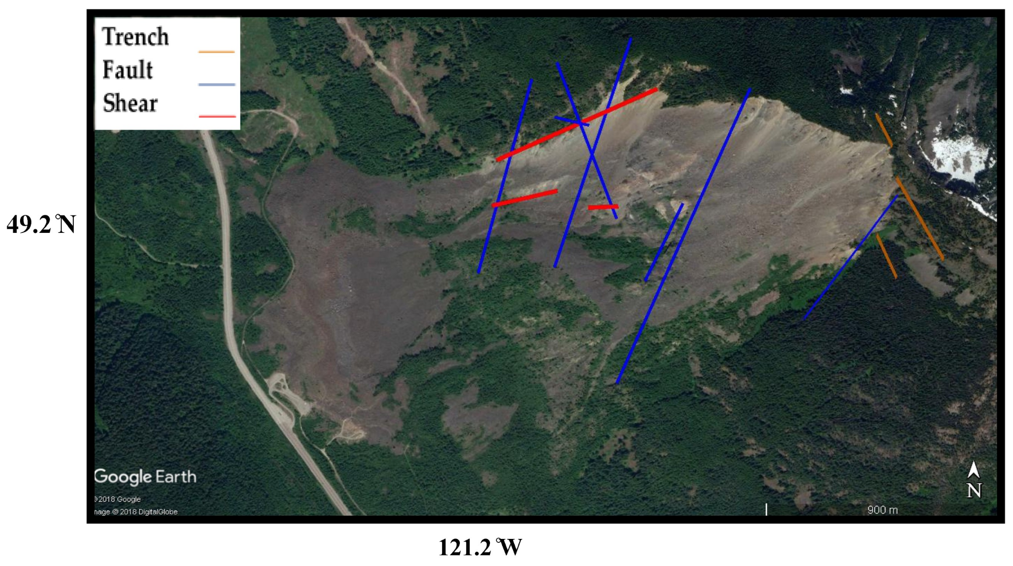
Three test sites (see Figure 1) that provide representative diversity for demonstrating the method enhancements are presented in the next section. Site characteristics for these case studies are shown in

Table 1. Case studies and their characteristics.

Test Site	Location	Description	Type of Risk	InSAR Observed Phenomena
1. Hope Slide	121.26°W 49.30°N	Slide scar (1965 landslide)	Unstable steep scar, major highway nearby	Strong deformation gradient near the headscarp. Evidence of rockfalls near sheer zone. Subtle movement in the accumulation zone. Deforming patch near the highway.
2. Mount Currie	122.78°W 50.25°N	Steep mountain ridge	Rockfall events, precursors to catastrophic landslide	Deformation near main tension cracks.
3. Boundary Range Slide	132°W 57.5°N	Compound rockslide	Slope instability, large scale movements recorded	Large scale movement at the bottom of the landslide (toppling zone). Sliding and transition zones are also detectable.

. The TSX-ST datasets for these three sites are summarized in

Table 2. Test sites and TerraSAR-X Staring Spotlight dataset (ascending (Asc.)/descending (Desc.)). (Incidence angles are expressed in degrees (deg), HH polarization refers to Horizontal transmit and Horizontal receive, and DSM is Digital Surface Model.).

Test Site	Time	No. Scenes	Orbit	Incidence (deg)	Polarization	Methods Demo
Hope Slide	August 2015–September 2017	8	Desc.	36	HH	Enhanced atmospheric correction
Mount Currie	June 2017–September 2017	6/6	Asc./Desc.	22/34	HH	Coherent layover topographic correction
Boundary Range Slide	June 2017–September 2017	8/8	Asc./Desc.	41/38	HH	Enhanced DSM blending

. Figure 2 shows the network of generated interferograms using the datasets of Table 2. The surface deformation maps of Section 4 are obtained, for each case study, using the interferogram in the network of Figure 2 with the least atmospheric contamination and the largest temporal baseline. If more than one interferogram in the network exhibits, comparable levels of atmospheric contamination, and temporal baselines, we selected the one with the smallest perpendicular baseline.

In the following, we describe the location and morphology of the sites, placing emphasis on the geological characteristics that make them suitable examples for the individual method enhancements.

2.1. Hope Slide

One of the largest landslides recorded in Canada occurred at this test side. The historic Hope Slide occurred in January 1965, in the Nicolum Valley in the Cascade Mountains near the municipality of Hope, British Columbia [8]. The landslide buried Highway 3 under 47 million cubic meters of rock [9]. Seven faults and three dominantly brittle shear zones, along with tension cracks and trench-like features, have been recognized as the main deformation features in the Hope Slide area [10,11]. The aforementioned geological features, along with the historical landslide in the Hope Slide, draws attention to using the TSX-ST images to perform a comprehensive analysis of slope stability on and around Hope Slide, to better understand the triggers and dynamics of mass movements in the area. Due to the topography of the area, the Hope Slide is exposed to strong turbulent mixing processes, atmospheric stratification, and changes in atmospheric pressure in time, which introduce significant atmospheric errors to these high resolution TSX-ST images [12]. Addressing and modelling the atmospheric effect (e.g., by means of the methodology described in Section 3.1 and Section 3.2) plays a key role in retrieving the deformation phase from the TSX-ST acquisitions for the Hope Slide.

2.2. Mount Currie

This test site comprises the northeast trending ridge above the village of Pemberton and Hamlet of Mount Currie, BC, Canada [13]. This site experienced a series of rockfall events near the ridge crest in 2015 and 2016. The rockfall activities, which may be precursors to a more catastrophic event associated with tectonic structures close to the Mount Currie ridgeline, raised concerns about the safety of human lives and infrastructure in the nearby communities. As Mount Currie’s deformation features (including rock slides, rockfalls, lineaments, and deep-seated gravitational slope deformation [14]) are also bringing about small-scale movements, the unprecedented spatial details of the TSX-ST can shed light on these movements and their mechanisms in Mount Currie. The challenge we need to face for using InSAR in such a rugged topography is shadow/layover effect, which decreases the quality of derived deformation maps from TSX-ST images. Even though the TSX-ST images have a high resolution, in a mountainous area with rugged topography, as with Mount Currie, the intractable geometrical distortions (shadow/layover) restrict the potential of repeat-pass InSAR. As a result, the methodology detailed in Section 3.3 is crucial to extracting additional information from the affected areas.

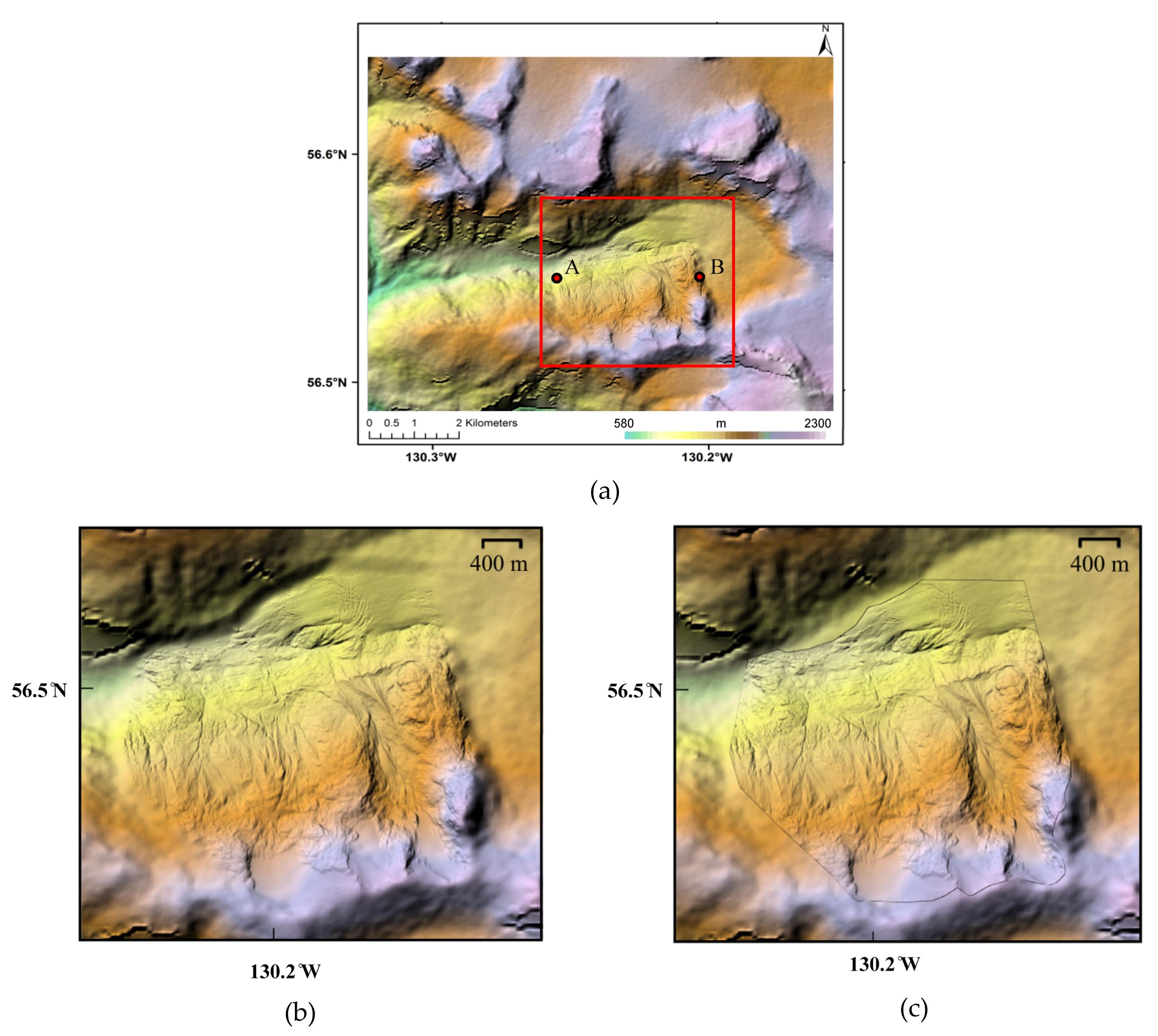
2.3. Boundary Range Slide

The Boundary Range Slide, located in the Coast Mountains of northwestern BC, Canada, has developed since 1956, when the bedrock started moved extensively and rapidly [15]. The retreat and downwasting of the Boundary Range Glacier appeared to have played a key role in the evolution of such a landslide. The investigations in 2008 showed that this landslide is approximately 1 km wide, 500 m long, and is actively deforming [16]. Clayton et al. [17], identified three geomorphic zones within the main landslide, including a lower zone that is toppling, an upper zone of sliding, and a transition zone of extension in between. As the area is changing very rapidly (0.8, 0.33, and 0.19 m/year for the toppling, transition, and sliding zones, respectively), an up-to-date high-resolution DSM is required to subtract the topographic and atmospheric contributions of the phase from the interferograms. To do so, we use a 2017 high resolution photogrammetric DSM (1 m) covering a small patch within the TSX-ST footprint. This DSM is merged with a low resolution Shuttle Radar Topography Mission (SRTM) extending over the whole area (30 m, generated in 2000) using the enhanced blending method described in Section 3.3.

3. Methods

In this section, we describe the developed individual enhanced methods for high-resolution InSAR processing, and how they integrate with the standard InSAR processing steps. Due to the current shortness of our InSAR time series, advanced stack-based InSAR methods cannot be used reliably, and “standard processing” here refers to basic pairwise InSAR (D-InSAR).

The D-InSAR phase, as the phase difference between two complex valued SAR images, can be decomposed as

$${\mathsf{\varphi }}_{\mathrm{int}}={\mathsf{\varphi }}_{\mathrm{def}}+{\mathsf{\varphi }}_{\mathrm{topo}}+{\mathsf{\varphi }}_{\mathrm{atm}}+{\mathsf{\varphi }}_{\mathrm{ref}}+{\mathsf{\varphi }}_{\mathrm{n}}.$$

(1)

The deformation term ${\mathsf{\varphi }}_{\mathrm{def}}$ accounts for temporal changes in phase occurring between the two acquisitions, e.g., due to surface movement or dielectric changes. The term ${\mathsf{\varphi }}_{\mathrm{topo}}$ is the topographic phase component due to difference in satellite orbit (spatial baseline) for the two acquisitions. ${\mathsf{\varphi }}_{\mathrm{atm}}$ is the phase component from propagation delays due to atmospheric water vapor variations in time and space. This quantity can be modelled as the sum of a “static” atmospheric term, which is a function of elevation, and a “dynamic” atmospheric term (based on the dynamic nature of the troposphere governed by minute-scale temporal variations of atmospheric water vapor largely at spatial scales > 3 km). The “flat earth” phase ${\mathsf{\varphi }}_{\mathrm{ref}}$ is proportional to the spatial baseline and the bald Earth ellipsoid, as seen by the side-looking SAR geometry. Finally, ${\mathsf{\varphi }}_{\mathrm{n}}$ accounts for any residual phase noise in the sensor electronics and due to temporal decorrelation of the imaged surface.

To obtain accurate surface displacement maps, ${\mathsf{\varphi }}_{\mathrm{def}}$ is estimated from the observed interferogram by appropriately modeling/estimating and compensating the other phase components in Equation (1). Standard methods to carry out the phase corrections to ${\mathsf{\varphi }}_{\mathrm{def}}$ are implemented in an automated python-based InSAR stack processing chain built on top of the Gamma software (e.g., [18]). Except for reference phase ${\mathsf{\varphi }}_{\mathrm{ref}}$, whose removal is uncontentious, we have developed enhancements for high spatial resolution data to the corresponding standard methods. These methods enhancements are detailed in the following subsections.

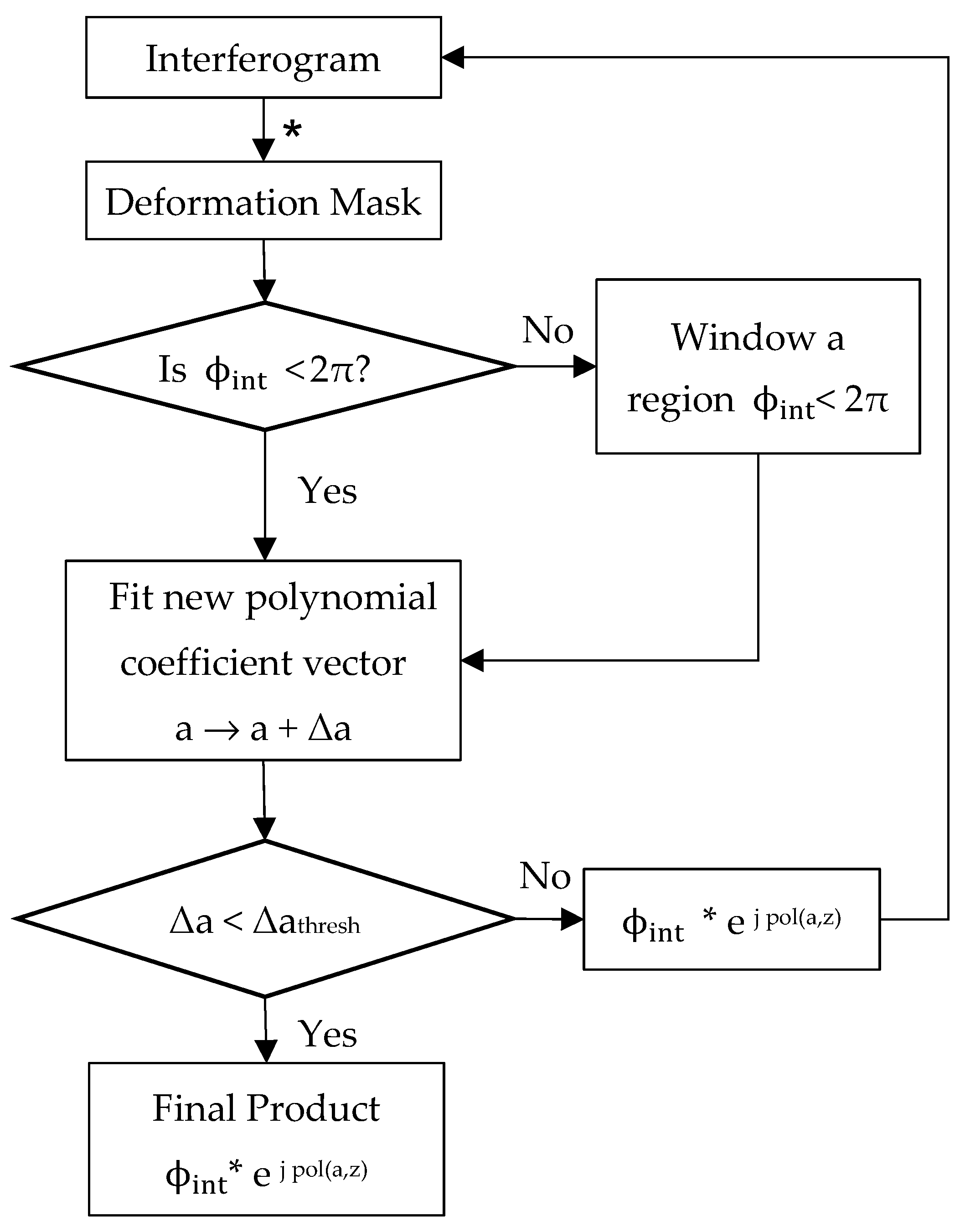
3.1. Atmospheric Phase Correction

Any changes of the troposphere (e.g., water vapor distribution and air pressure) between the two acquisitions of an interferogram lead to a phase error component ${\mathsf{\varphi }}_{\mathrm{atm}}$. If the atmosphere is at rest at the time of a SAR acquisition, the equations of motion become [8]

$$\begin{gathered} 0=\frac{-1}{\mathsf{\rho }}\frac{\partial \mathrm{P}}{\partial \mathrm{x}}, \\ 0=\frac{-1}{\mathsf{\rho }}\frac{\partial \mathrm{P}}{\partial \mathrm{y}}, \\ \mathrm{g}=\frac{-1}{\mathsf{\rho }}\frac{\partial \mathrm{P}}{\partial \mathrm{z}}, \end{gathered}$$

(2)

with P atmospheric pressure, $\mathsf{\rho }$ air density, $\mathrm{g}$ gravity, and x, y, z being easting, northing, and elevation, respectively. Equation (2) shows that for a static atmosphere, P depends on z only. As a consequence, the static atmospheric contribution of ${\mathsf{\varphi }}_{\mathrm{atm}}$, which is proportional to the pressure difference between the SAR acquisitions forming the interferogram, will also be a function solely of z [9]. For most atmospheric conditions, this function is an exponential that is well approximated by a linear or quadratic polynomial, pol(a,z), with coefficient vector a. In contrast to the static contribution, which depends on elevation, the dynamic contribution to ${\mathsf{\varphi }}_{\mathrm{atm}}$ is proportional to the difference in the random turbulent patterns of moving water vapor at the SAR acquisition times. While these patterns are hard to predict or model, they have little spatial energy at scales below 5 km [19], which separates them from most of the landslide displacement patterns we want to measure, which occur at scales of 1 km or less.

According to [20,21], a linear or a power-law relationship between the phase and topography can be assumed to correct for the atmospheric correction from the high-resolution interferometric phase. Therefore, we implemented a method to estimate both the static and dynamic part of ${\mathsf{\varphi }}_{\mathrm{atm}}$ using correlation analysis between the phase of atmospheric-contaminated interferograms and ground elevation from an accurate high-resolution DSM via the iterative algorithm detailed in Figure 3. Areas of suspected movement are masked from the interferogram, which is segmented into overlapping tiles of ~0.5 km × 0.5 km. The algorithm in Figure 3 is carried out for each tile. In a first iteration, the coefficients are found by least squares fitting over an area of the interferogram tile. The support area for the fit must have a small enough elevation diversity to contain the atmospheric phase component safely within one 2π interval, to prevent incorrect fitting of wrapped phase values. In a second iteration, the coefficient vector, a, can be refined by adding a correction (Δa) via fitting the phase residual after removing pol(a,z) found in the first step. As the dynamic range of the phase residual is diminished compared to the original phase, the support area and elevation diversity can be increased in the second step, which increases the accuracy of the polynomial fit. Iterations are continued until Δa falls below a predefined threshold. For each tile, the constant coefficient of the polynomial (phase offset) is interpreted as the average dynamic phase of the tile, while the higher order coefficients are interpreted as describing the static phase contribution. The phase offsets of these overlapping tiles are then interpolated to generate a smooth phase screen over the scene.

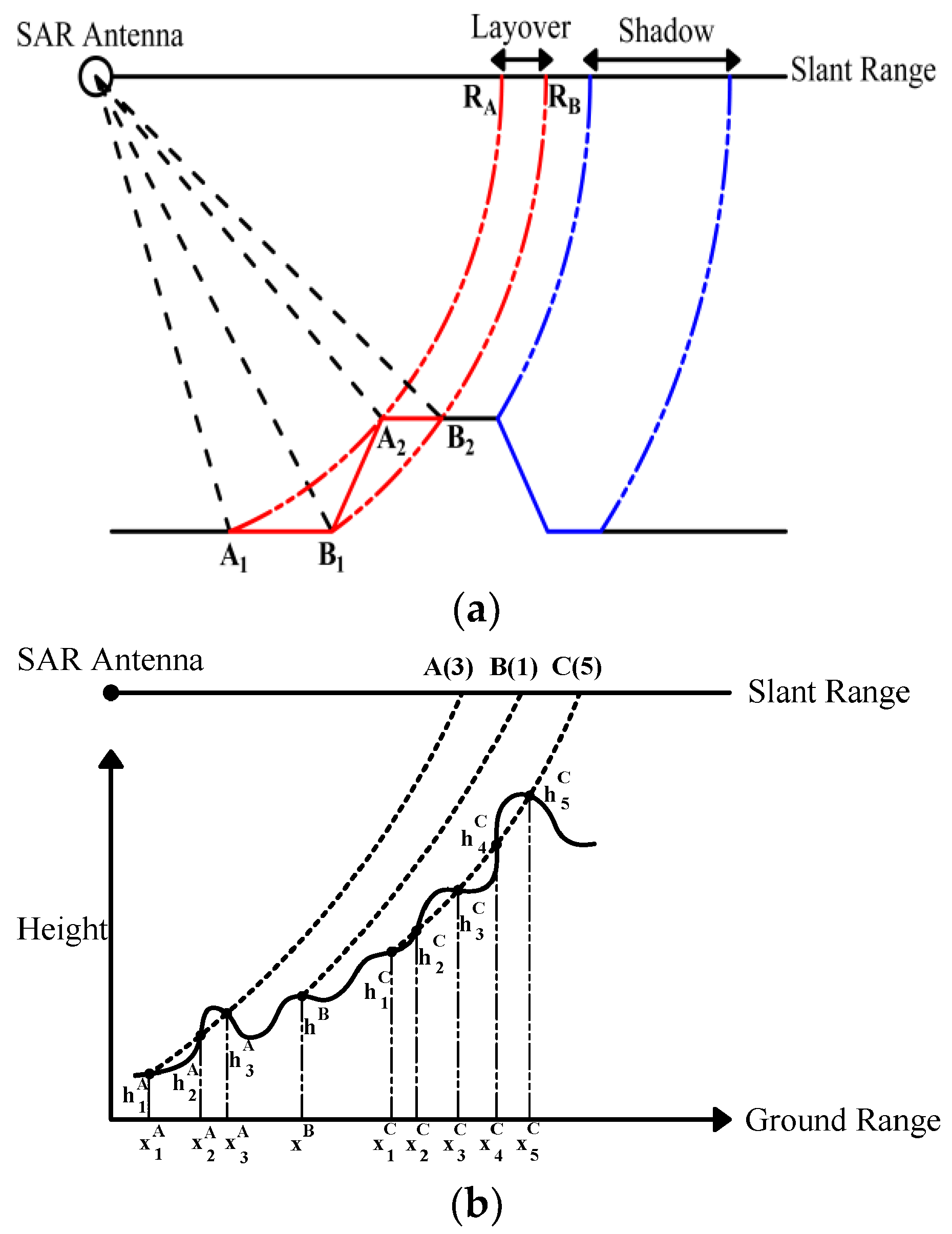
3.2. Layover Topographic Correction Method

Due to the SAR side-looking geometry, whenever the terrain slope exceeds the incidence angle, more than one area on the ground contributes to the backscatter of a single resolution cell in the SAR image; this is the well-known layover effect [22] (Figure 4a). In layover areas, InSAR produces a superimposed phase whose decorrelation properties are governed by volume coherence criteria even if the scattering mechanisms are all purely from surface scattering. In particular, there is a much faster decorrelation with spatial baseline than for non-layover regions. However, for most current space-borne sensors, the orbital tubes, and thus maximum spatial baselines, are typically kept small, and layover areas, particularly in high resolution images, are often sufficiently coherent to produce an InSAR phase that is at least theoretically usable. Steep and rugged mountainous terrain in high-resolution SAR generally exhibits a significant number of disjointed layover areas as incidence angle cannot be chosen too large, to avoid shadowing. In order to exploit coherent layover phase for detecting ground movement, one needs to model the superposition of the phase from its different ground contributions, and to carry out the topographic phase corrections correspondingly [23,24,25,26,27]. Ground motion can be detected and attributed to a unique area on the ground only when there is a dominant (as revealed by the superposition modeling) phase contribution in the layover. For this study, we have introduced a simple new technique to topographically correct the phase in layover areas for this case based on an accurate SAR geometry and a high-resolution DSM (such as from photogrammetric DSM). The ray-tracing concept of the technique is shown in Figure 4b.

The technique consists of two steps. First, we construct a series of line-of-sight (LOS) vectors from the sensor to the DSM for every (zero-Doppler) range line of the SAR image as a function of look angle, which is measured at the sensor with respect to its state vector. This delivers both elevation and slant range, which are calculated as the length of the look vector, and series as a finally-sampled function of the look angles. Sections of the range line that are not illuminated by the SAR, due to shadow, are first found and marked via ray tracing as a binary illumination mask matching the series. The slant range series is then converted to a non-integer slant range pixel, and together with the illumination mask, is used to find all elevations, their corresponding ground locations, and the local incidence angles that share the same integer slant range pixel. The result is stored in a suitable numerical structure. Then, the second step analyzes this result in terms of a simple relative contribution, making up the backscatter of the non-unique layover pixels. This uses the local incidence angles of the contributions assuming a cosine scattering law [28] and constant surface roughness. If one of the ground areas dominate the backscatter (intensity > 75 percent of total), we assign the corresponding elevation and ground location to the slant range DSM and geocoding look-up table, respectively. A further sophistication currently being implemented is to use actual geocoded backscatter interpolated from only the uniquely locatable slant range pixels to estimate the individual backscatter contributions making up the non-unique pixels. By reducing the initial topographic phase error, our method also will improve performance of future InSAR time series analysis in coherent layover areas. The extra height error correction in layover found through time series decomposition [29,30] will be usable also as an a posteriori measure of validity for the backscatter superposition model of the just-presented topographic correction method, and consequently, also of the geolocation of the residual deformation phase.

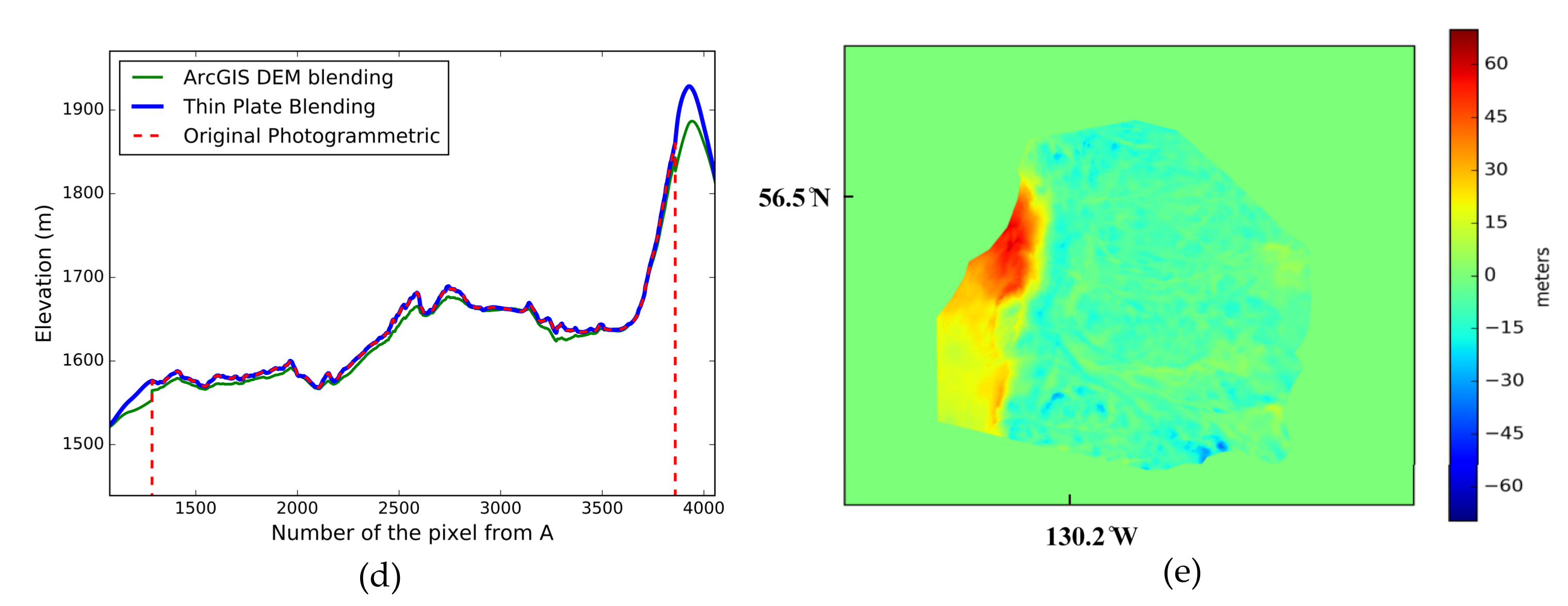
3.3. Digital Surface Model Blending Method

The quality of the topographic correction of the D-InSAR phase ${\mathsf{\varphi }}_{\mathrm{topo}}$ depends highly on the accuracy of the DSM used. Baseline-dependent errors in the deformation phase stemming from DSM inaccuracies can be removed via time series analysis [31], but for shorter series, particularly the simple D-InSAR case, it is crucial to use as good a DSM surface as can be constructed. A standard problem is the merging of continuous existing DSMs with lower resolution and accuracy (such as SRTM) with newer higher resolution DSMs (often from photogrammetry and Light Detection and Ranging (LiDAR)) to generate the DSM surface used by the InSAR processing chain [32]. To avoid artifacts in the topographically-corrected phase across where DSMs were joined together, smooth/differentiable transitions are desirable. For the standard InSAR case of merging two or more DSMs, there is usually a clear hierarchy of trustworthiness, which suggests that the older coarse resolution DSM should be altered and matched to the newer high-resolution DSM at their boundary, while the latter should remain unaltered. By contrast, the state-of-the-art algorithms we are aware of (e.g., [33]) only allow merging of DSMs through symmetric blending. We, therefore, developed a simple new method based on thin-plate spline fitting, that “molds” the coarse DSM to the unaltered high-resolution DSM, while also minimizing any distortions and stitching errors along the boundaries during the blending procedure. The concept of the new method is shown in Figure 5.

The method consists of two steps that are described below:

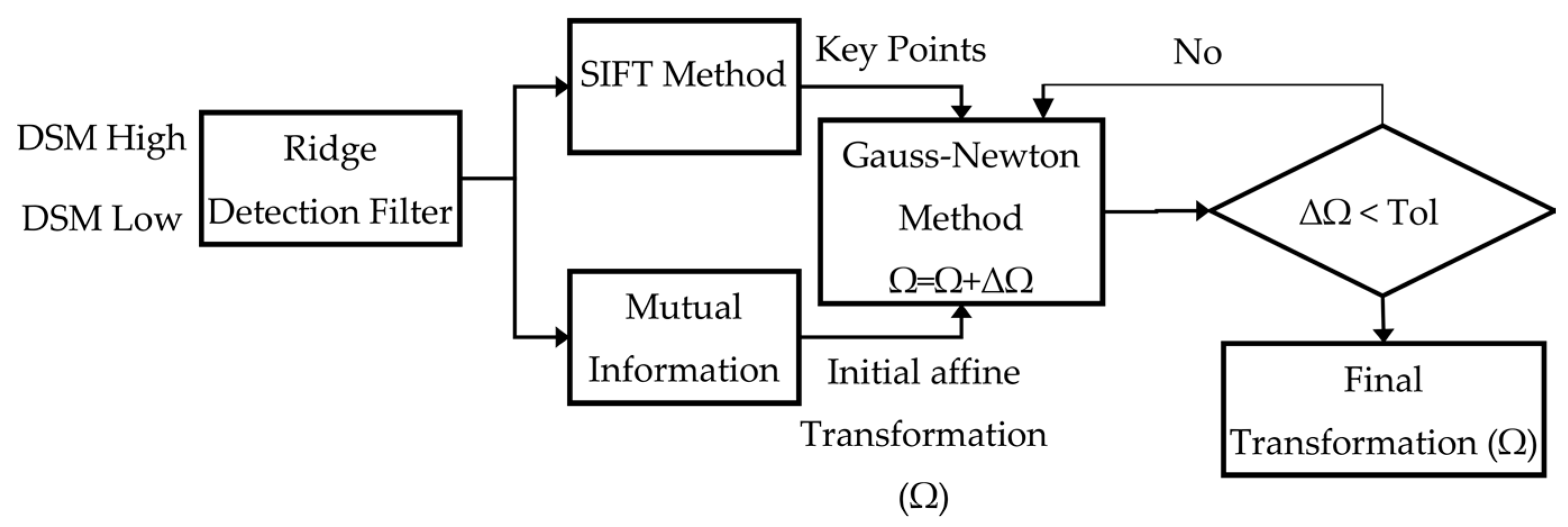
• Step one is to co-register the high- and low-resolution DSM in the overlapping area to find and fix any potential datum issues, elevation offsets, horizontal shifts, or rotations, etc. To do so, for each DSM, we derived feature points along the ridgelines by calculating and thresholding the ratio between the large and the small eigenvalue of the Hessian matrix. Mutual information method [34,35] is used to calculate the initial translation and rotation components of the affine transformation between the two DSMs. To refine, first correspondence between the two sets of feature points is established using the scale-invariant feature transform (SIFT [36]). Based on this feature pair list, the Gauss–Newton method [37] is used to refine the affine transformation parameters iteratively.
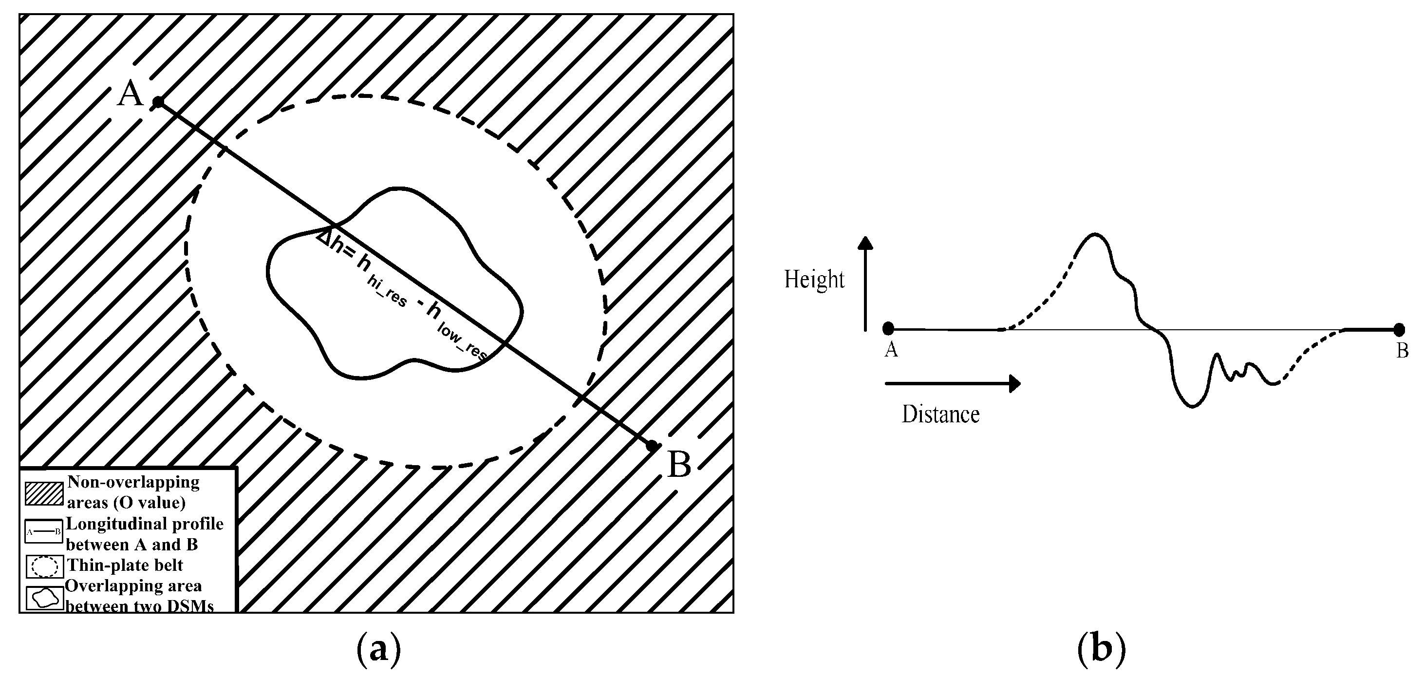
• Step two defines a belt-shaped region of width between 100 to 150 postings of the coarse DSM (Figure 6) surrounding the high-resolution DSM(s). A thin plate spline is then fitted across this belt, with clamped boundary conditions of ∆h = h_highres − h_lowres at the inner edge (=boundary of the high-resolution DSM) and 0 at the outer edge of the belt. The result of this fit is a correction surface that is subtracted from the coarse DSM. The so-corrected coarse DSM can then be seamlessly merged with the high-resolution DSM by simply inserting the latter into the former.

4. Results and Discussion

The methods detailed in Section 3 are now applied to the three test sites presented in Section 2 to generate accurate surface deformation maps. The results of this study are illustrated and discussed in the following.

4.1. Hope Slide

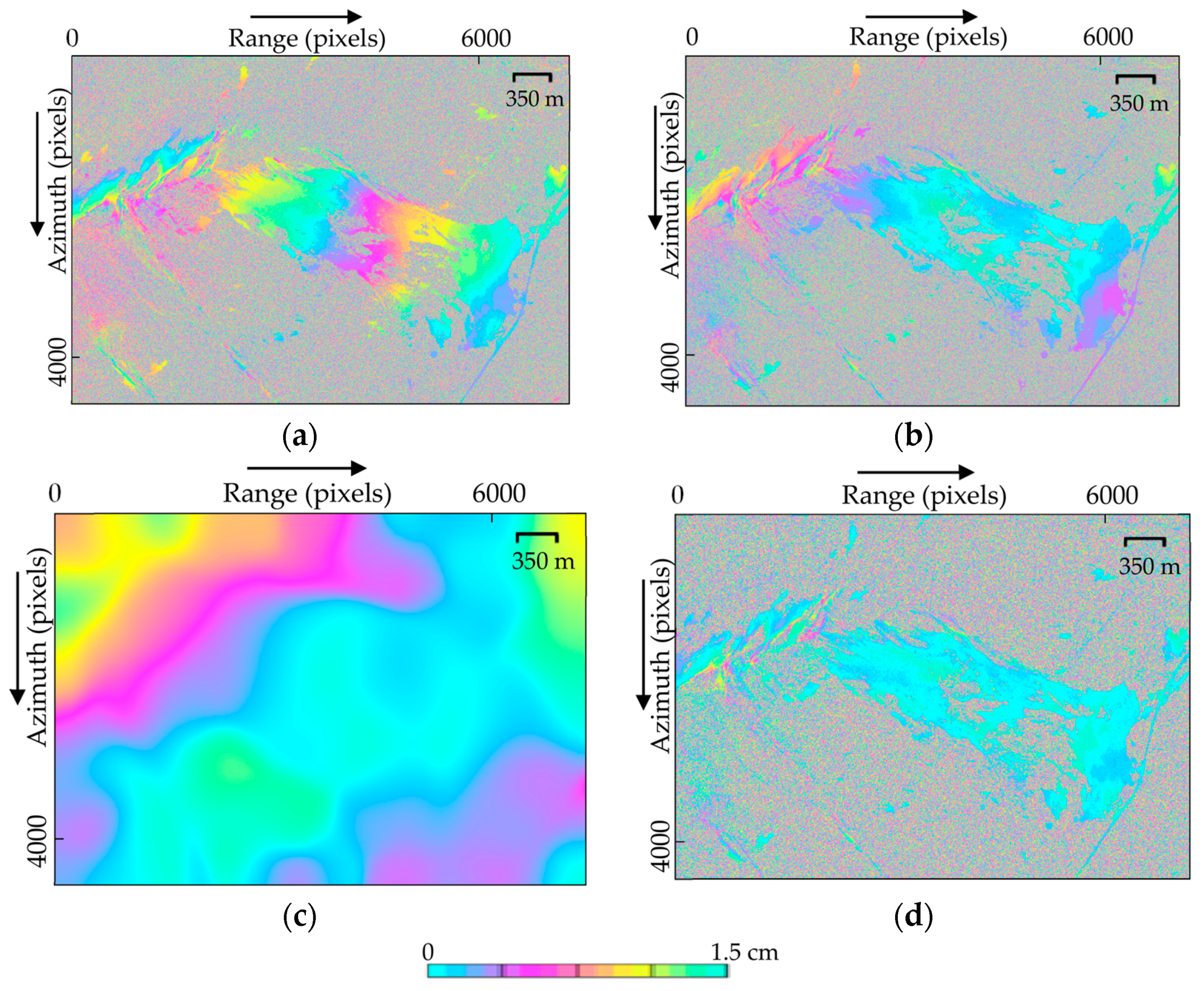
4.1.1. Atmospheric Phase Correction

As highlighted in Section 2.1, we expect the Hope Slide interferograms to be influenced considerably by atmospheric changes due to the topography of the area (see

Table 3. Hope Slide presented interferograms.

Section Demo	Pair	Orbit	Incidence (deg)	Polarization	Perp. Baseline (m)	Weather
Atmospheric phase correction	21 June 2015	Desc.	36	HH	45	Cloudy, 10 °C
	4 August 2015					Foggy, 14 °C
Surface deformation map	15 August 2015	Desc.	36	HH	160	Clear, 13 °C
	23 September 2017					Partly Cloudy, 16 °C

). For instance, the phase pattern of the Hope Slide interferogram shown in Figure 7a (June to August 2015) is indicative of pronounced atmospheric effects that, if not corrected, would significantly affect the accuracy of the estimated surface deformation. The procedure detailed in Section 3.1 and Section 3.2 is applied to mitigate the phase induced from both static atmosphere (Figure 7b) and dynamic atmosphere Figure 7c). A remarkable reduction of the atmospheric-induced effects can be observed by comparing the interferograms before (Figure 7a) and after (Figure 7d) atmospheric correction.

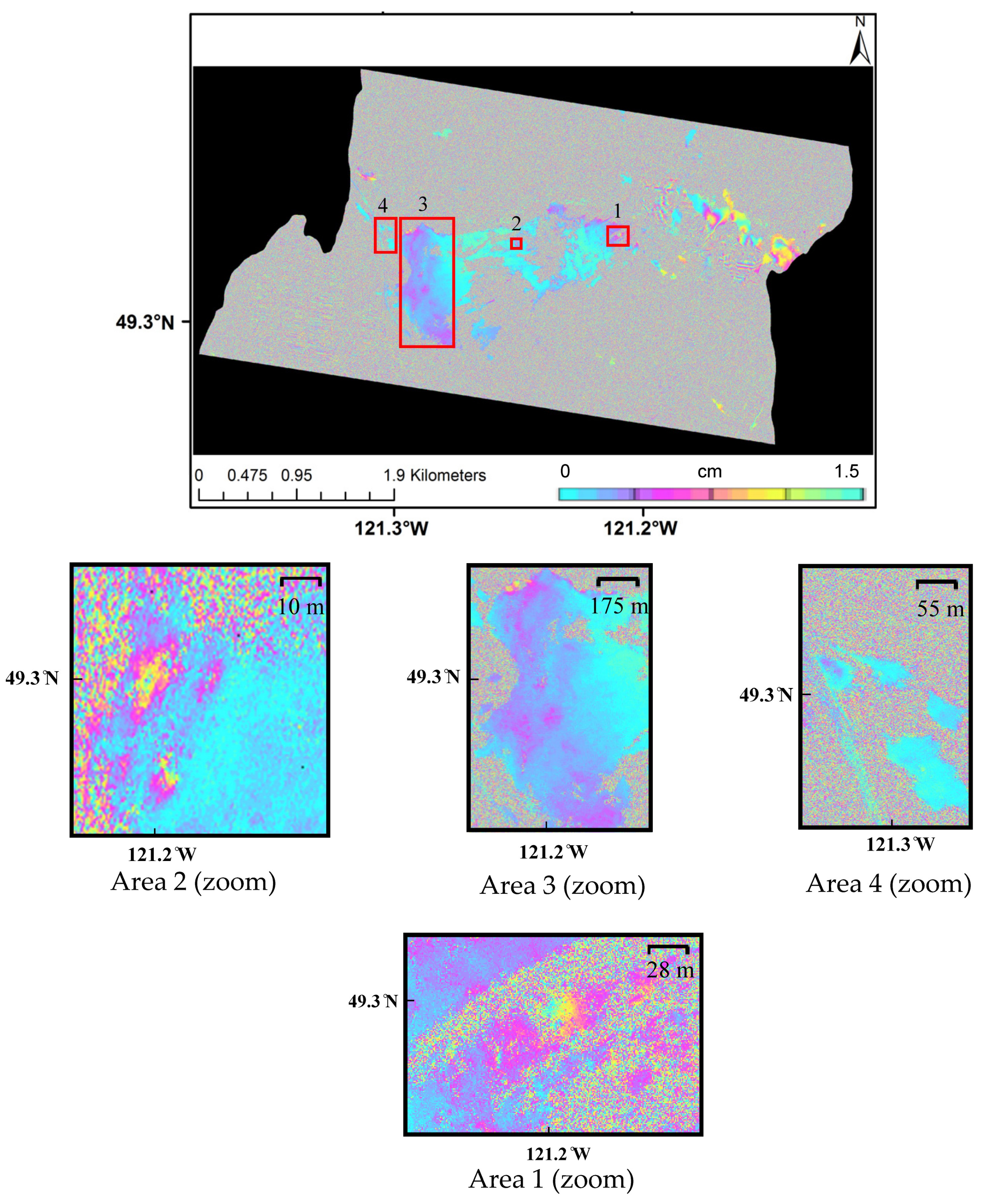
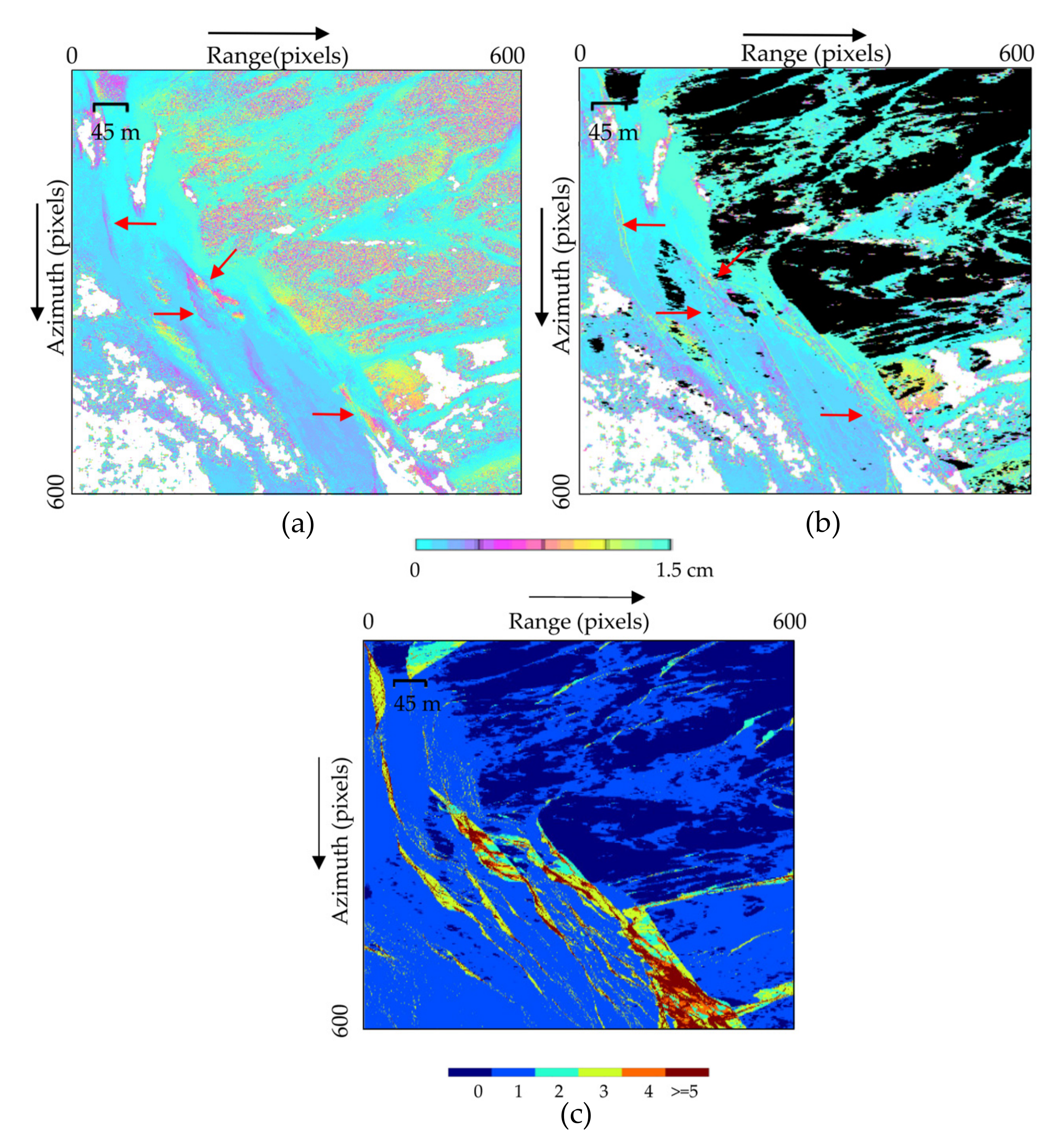
4.1.2. Surface Deformation Map

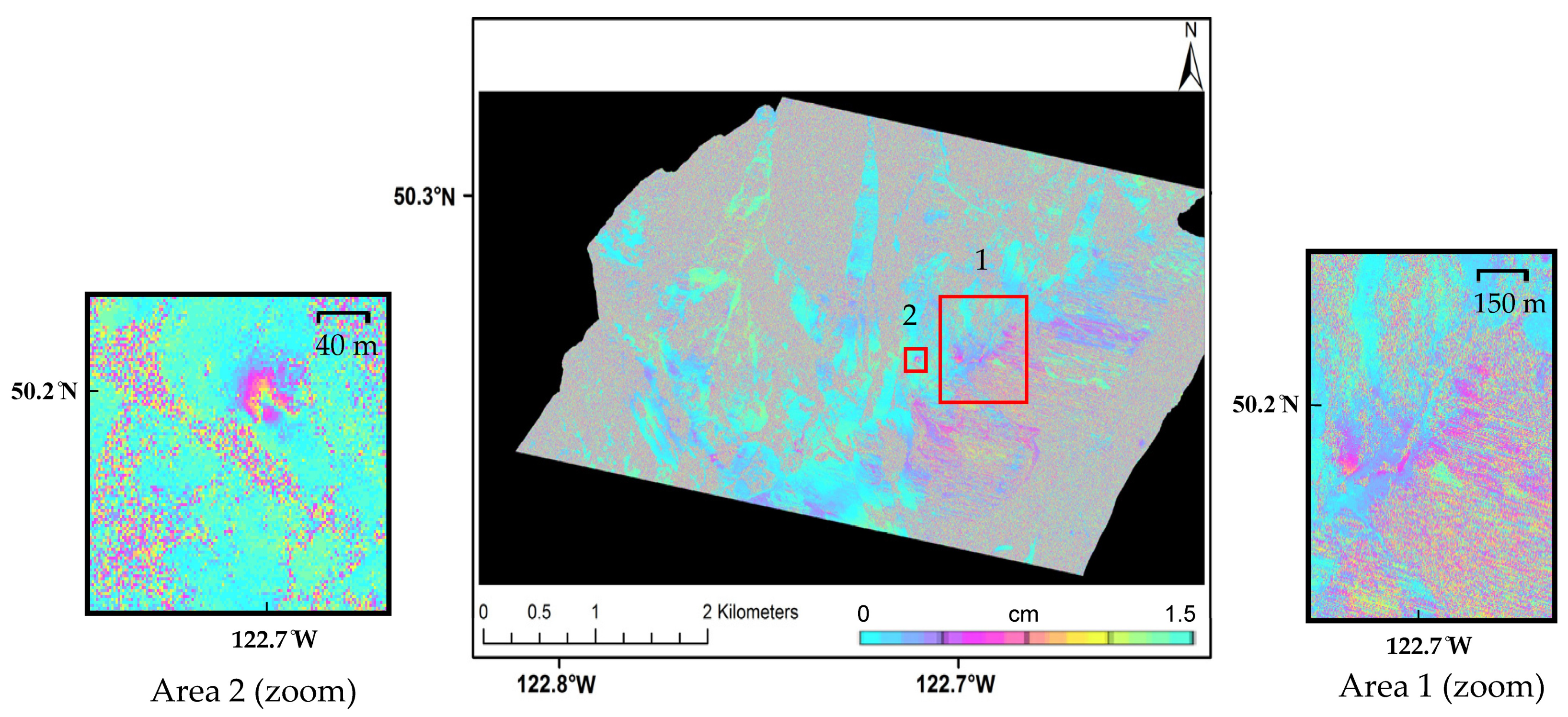
Figure 8 shows an atmospherically corrected interferogram, August 2015 to September 2017, spanning close to the maximum observed time period (see Table 3). The spatial baseline of this interferogram is approximately 160 m. Despite having a relatively large spatial baseline, this interferogram has the least dynamic atmospheric contamination and the largest temporal baseline. In the same figure, four areas with small-scale deformation are highlighted in red, with the corresponding zoom insets displayed on either side.

The first inset shows a newly identified area with rockfall potential near the headscarp of the Hope Slide. The most evident deformation feature is a small region containing a full interferometric color fringe indicative of a strong deformation gradient. The second inset shows another similar active part of the landslide. The concentration of the regional tectonic features, such as faults and shear zones (Figure 9), which reduce the quality of rock mass [11], can cause onset of rockfalls or slides compatible with the deformation pattern observed in the interferogram. The third inset shows subtle movement in the accumulation zone of the Hope Slide, where the debris of the historic landslide has accumulated and created a bulge. The interferogram suggests subtle movement away from the SAR sensor and along the LOS direction for this region. This movement may indicate secondary slides in the deposits of the historic landslide, or alternatively, subsidence/settling of the bulge.

The fourth inset shows a small deforming patch located near the highway. This area corresponds to the distal edge of the coarse portion of the 1965 Hope Slide deposit. As the movement is observed in the LOS direction, there are two possible deformation scenarios: either the landslide deposit might be subject to subsidence on its eastern side, or the eastern side of the hill is experiencing a slow landslide. Although the deformation is subtle in this zone, at its current rate, it may lead to minor damage to road prism and the need for maintenance.

4.2. Mount Currie

4.2.1. Layover Topographic Correction

As discussed in Section 2.2, all Mount Currie interferograms are expected to be affected by small-scale dissected layover, owing to rugged topography and steep incidence angle. The method of Section 3.2 is therefore applied to all interferograms in order to topographically correct the phase in layover areas. The algorithm allows for pinpointing of areas whose non-zero residual phase in the original interferogram is caused by erroneous topographic correction inside layover/shadow areas, rather than actual deformation.

In Figure 10, we demonstrate the performance of the proposed layover topographic correction method for a layover-affected subregion of an 11-day interferogram with a spatial baseline of 21 m (see

Table 4. Mount Currie presented interferograms.

Section Demo	Pair	Orbit	Incidence (deg)	Polarization	Perp. Baseline (m)	Weather
Layover topographic correction	24 July 2017	Desc.	34	HH	21	Clear, 28 °C
	4 August 2017					Clear, 26 °C
Surface deformation map	2 July 2017	Desc.	34	HH	5	Clear, 27 °C
	6 September 2017					Windy, 18 °C

). A comparison of the interferograms before and after correction (Figure 10a,b), respectively) shows a number of layover artifacts in the original interferogram (highlighted with red arrows in Figure 10a) as well as shadow-affected areas that are now corrected and masked out.

4.2.2. Surface Deformation Map

Figure 11 shows a 66-day interferogram spanning the period 2 July to 6 September 2017. Besides a negligible residual atmospheric phase for both acquisitions of the pair, this interferogram also has the smallest spatial baseline (5 m) and longest possible temporal baseline achievable with our data to date. Details about this pair are available in Table 4.

Surface movements are observed in two areas on the northern face of Mount Currie. The first region, which is situated along the ridge east of Currie, is a source for potential rock avalanches according to BGC Engineering report [14]. The interferogram indicates ongoing deformation in this area, which encompasses the main tension cracks. The deformation observed in the interferogram is consistent with the deformation pattern previously documented in this area [13]. The high quality information of this interferogram suggests a rock avalanche precursor motion, which, if it happens, might dam Green and Lillooet rivers and damage the airport [14]. The second area shows another noticeable block movement occurring near a zone characterized by a deep-seated gravitational slope deformation delimited by tension cracks. The observed movement suggests the potential of rockfalls in this zone.

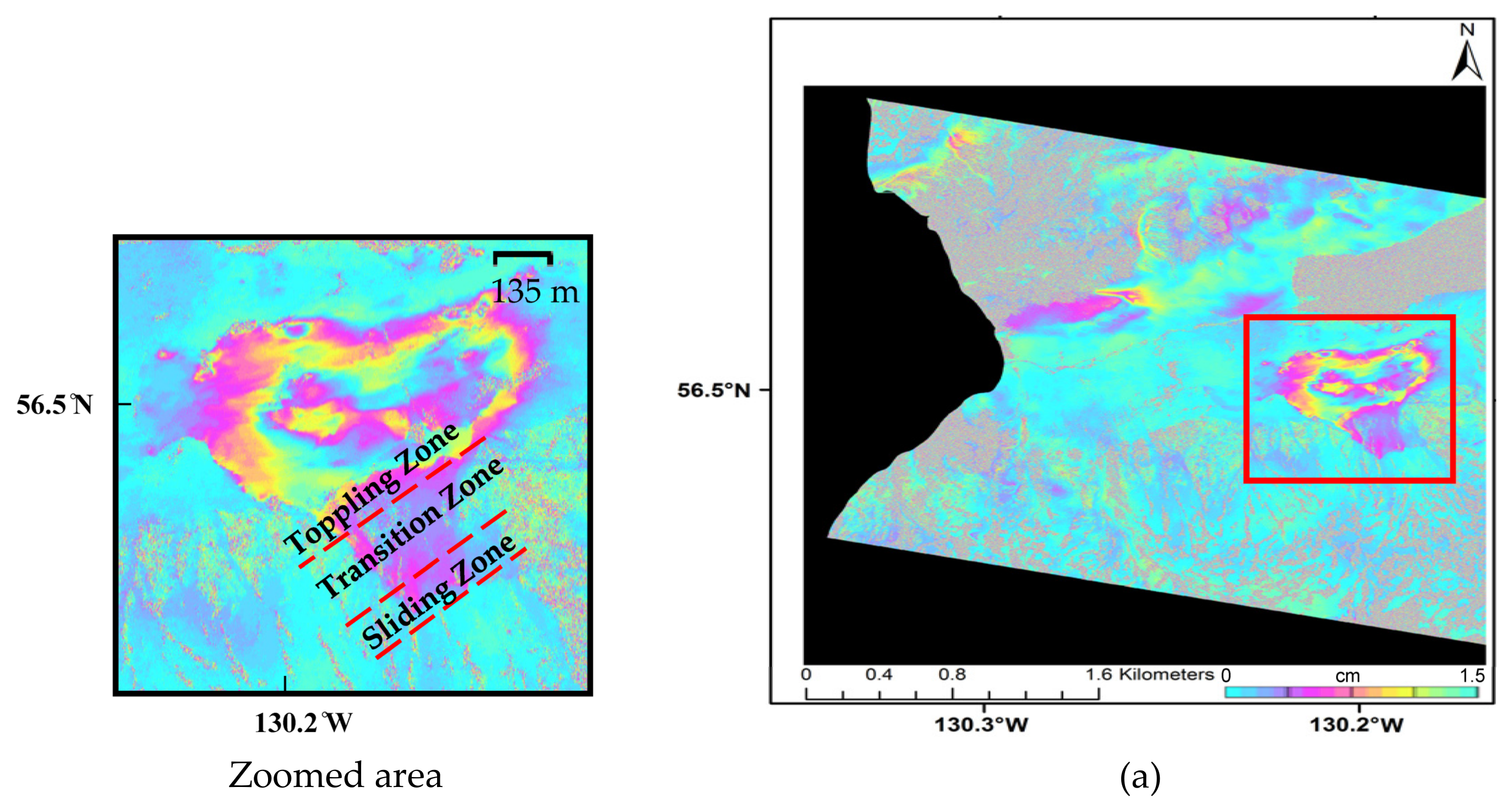
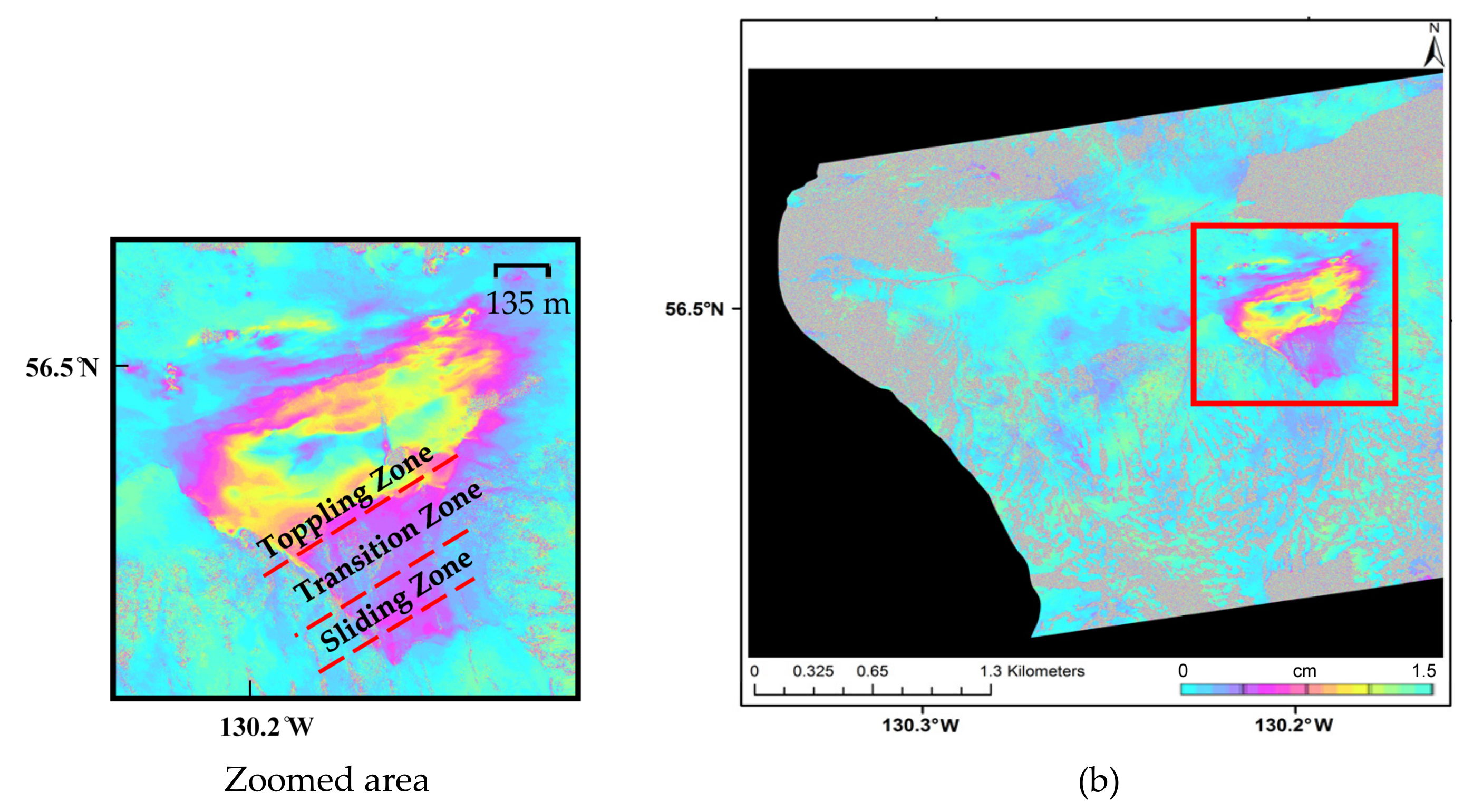
4.3. Boundary Range Slide

4.3.1. Digital Surface Model Blending

With respect to high deformation rate and ongoing glacial retreat in the Boundary Range Slide, it is essential to use an updated high-resolution DSM for the InSAR processing. To update the existing DSM of the area (SRTM, 30 m resolution), we merged the latter with a more recent high-resolution photogrammetric DSM (1 m) covering a small patch within the radar footprint using the thin-plate blending method detailed in Section 3.3.

The shaded relief of the generated DSM is displayed in Figure 12a. For comparison, we also computed a second DSM by blending photogrammetric and SRTM DSMs via a conventional amalgamation approach implemented in ArcGIS software. This approach takes the average of the two DSMs in the overlapping areas and along the boundaries to generate a smoother blended DSM. A small patch of each DSM has been selected over the highlighted area in Figure 12a, and is presented in Figure 12b,c to visually compare them.

The elevation profile for a transect of both blended DSMs (i.e., between A and B, see Figure 12a), plotted in Figure 12d, indicates good agreement between photogrammetric and thin-plate blended DSM, confirming that the proposed method is only altering the lower resolution DSM, leaving the high-resolution DSM intact. When using the conventional approach, on the other hand, one can observe pronounced differences between photogrammetric and blended DSM (error up to 62 m, see Figure 12e) owing to the symmetric smoothing of the high- and low-resolution DSMs, regardless of their substantial differences in acquisition dates and resolutions. In addition to that, the conventional approach generates noticeable discontinuities/wrong elevations at the boundaries between low- and high-resolution DSMs (Figure 12c).

4.3.2. Surface Deformation Map

The ascending and descending interferograms in Figure 13 are characterized by a very small spatial baseline (i.e., 27 m and 33 m respectively), and a temporal baseline that is close to the maximum that the study allows (i.e., 66 days, from June to September 2017). These interferograms have also a negligible identified residual atmospheric phase for both acquisitions of the two pairs (details in

Table 5. Boundary Range Slide presented interferograms.

Section Demo	Pair	Orbit	Incidence (deg)	Polarization	Perp. Baseline (m)	Weather
Surface deformation map	30 June 2017	Desc.	38	HH	33	Cloudy, 15 °C
	4 September 2017					Mainly Clear, 21 °C
Surface deformation map	29 June 2017	Asc.	41	HH	27	Cloudy, 17 °C
	3 September 2017					Clear, 18 °C

).

Surface movement is observed in one major area (highlighted in red in Figure 13). Owing to the high resolution of ST-TSX data, the approximate boundaries of the sliding, transition, and toppling zones of the Boundary Range Slide are recognizable based on their rates of deformation (see the zoom insets in Figure 13). The location of the Boundary Range Slide main scarp, which forms the upper boundary of the sliding zone, is clearly detectable in the interferograms. The interferometric phase further shows large scale movement at the bottom of the landslide area corresponding to the toppling zone as the fastest moving part of the slide identified by previous studies [16]. The transition zone is also detectable in the interferograms, separating the two abovementioned areas.

5. Conclusions

This study presents three enhanced processing methods developed for high resolution InSAR data to improve the estimation of surface deformation. The first method aims to compensate for the InSAR phase induced by static and dynamic atmosphere by fitting a linear model to phase and relative height from a DSM for each pixel of the interferogram. The second method aims to correct the InSAR phase over layover-affected areas based on SAR geometry and high-resolution DSMs. The third method blends low- and high-resolution DSMs by molding the former to match the latter at the boundaries using thin plate spline fitting.

The proposed algorithms demonstrate using TerraSAR-X Staring Spotlight datasets over three sites in BC having geological characteristics that make them representative end-members for this study. Performance comparisons between original and corrected interferograms show that the proposed methods significantly improve the final interferometric deformation maps by removing the non-deformation phase components. High coherence and unprecedented spatial detail of the results indicate excellent suitability of TerraSAR-X Staring Spotlight data for identification and monitoring small-scale landslides in challenging mountainous areas.

The observed movements in line-of-sight direction of the satellite reveal that all the test sites are susceptible to future rockfalls at small and large scales. Therefore, continued assessment of the sites with high resolution InSAR over longer time periods is expected to quantify the likelihood of larger events, such as rock avalanches or landslides, to help avoid future losses.

References

1. Jakob, M.; Lambert, S. Climate change effects on landslides along the southwest coast of British Columbia. Geomorphology 2009, 107, 275–284. [Google Scholar] [CrossRef]
2. Soldati, M.; Corsini, A.; Pasuto, A. Landslides and climate change in the Italian Dolomites since the late glacial. Catena 2004, 55, 141–161. [Google Scholar] [CrossRef]
3. Curlander, J.C.; McDonough, R.N. Synthetic Aperture Radar; John Wiley & Sons: New York, NY, USA, 1991; Volume 396. [Google Scholar]
4. Bamler, R.; Hartl, P. Synthetic aperture radar interferometry. Inverse Probl. 1998, 14, R1. [Google Scholar] [CrossRef]
5. Krieger, G.; Moreira, A.; Fiedler, H.; Hajnsek, I.; Werner, M.; Younis, M.; Zink, M. Tandem-x: A satellite formation for high-resolution sar interferometry. IEEE Trans. Geosci. Remote Sens. 2007, 45, 3317–3341. [Google Scholar] [CrossRef] [Green Version]
6. Carrara, W.G.; Goodman, R.S.; Majewski, R.M. Spotlight Synthetic Aperture Radar; Artech House: Norwood, MA, USA, 2007. [Google Scholar]
7. Mittermayer, J.; Wollstadt, S.; Prats-Iraola, P.; Scheiber, R. The TerraSAR-X staring spotlight mode concept. IEEE Trans. Geosci. Remote Sens. 2014, 52, 3695–3706. [Google Scholar] [CrossRef]
8. Donati, D.; Stead, D.; Brideau, M.; Ghirotti, M. A remote sensing approach for the derivation of numerical modelling input data: Insights from the Hope Slide, Canada. In ISRM AfriRock—Rock Mechanics for Africa; Internation Society for Rock Mechanics and and Rocke Engineering: Cape Town, South Africa, 2017. [Google Scholar]
9. Mathews, W.; McTaggart, K. Hope rockslides, British Columbia, Canada. In Developments in Geotechnical Engineering; Elsevier: New York, NY, USA, 1978; Volume 14, pp. 259–275. [Google Scholar]
10. Von Sacken, R.S. New Data and Re-Evaluation of the 1965 Hope Slide, British Columbia. Ph.D. Thesis, University of British Columbia, Vancouver, BC, Canada, 1991. [Google Scholar]
11. Brideau, M.-A.; Stead, D.; Kinakin, D.; Fecova, K. Influence of tectonic structures on the Hope Slide, British Columbia, Canada. Eng. Geol. 2005, 80, 242–259. [Google Scholar] [CrossRef]
12. Ding, X.-L.; Li, Z.-W.; Zhu, J.-J.; Feng, G.-C.; Long, J.-P. Atmospheric effects on InSAR measurements and their mitigation. Sensors 2008, 8, 5426–5448. [Google Scholar] [CrossRef] [PubMed]
13. Bovis, M.J.; Evans, S.G. Rock slope movements along the Mount Currie “fault scarp,” southern coast mountains, British Columbia. Can. J. Earth Sci. 1995, 32, 2015–2020. [Google Scholar] [CrossRef]
14. BGC Enginnering Inc. Mount Currie Landslide Risk Assessment; BGC Enginnering Inc.: Vancouver, BC, Canada, 2018. [Google Scholar]
15. Clayton, M.; Stead, D.; Kinakin, D. The Mitchell Creek landslide, BC, Canada: Investigation using remote sensing and numerical modeling. In Proceedings of the 47th US Rock Mechanics/Geomechanics Symposium, San Fransisco, CA, USA, 23–26 June 2013. [Google Scholar]
16. Clayton, M.A. Characterization and analysis of the Mitchell Creek Landslide: A Large-Scale Rock Slope Instability in Northwestern British Columbia. Ph.D. Thesis, Science: Department of Earth Sciences, Cambridge, UK, 2014. [Google Scholar]
17. Clayton, A.; Stead, D.; Kinakin, D.; Wolter, A. Engineering geomorphological interpretation of the Mitchell Creek landslide, British Columbia, Canada. Landslides 2017, 14, 1655–1675. [Google Scholar] [CrossRef]
18. Werner, C.; Wegmüller, U.; Strozzi, T.; Wiesmann, A. Gamma SAR and interferometric processing software. In Proceedings of the ERS-Envisat Symposium, Gothenburg, Sweden, 16–20 October 2000; p. 1620. [Google Scholar]
19. Rabus, B.T.; Ghuman, P.S. A simple robust two-scale phase component inversion scheme for persistent scatterer interferometry (dual-scale psi). Can. J. Remote Sens. 2009, 35, 399–410. [Google Scholar] [CrossRef]
20. Bekaert, D.; Hooper, A.; Wright, T. A spatially variable power law tropospheric correction technique for insar data. J. Geophys. Res. Solid Earth 2015, 120, 1345–1356. [Google Scholar] [CrossRef]
21. Bekaert, D.; Walters, R.; Wright, T.; Hooper, A.; Parker, D. Statistical comparison of InSAR tropospheric correction techniques. Remote Sens. Environ. 2015, 170, 40–47. [Google Scholar] [CrossRef]
22. Kwok, R.; Curlander, J.C.; Pang, S.S. Rectification of terrain induced distortions in radar Imagery. Photogramm. Eng. Remote Sens. 1987, 53, 507–513. [Google Scholar]
23. Jakowatz, C.V.; Thompson, P. A new look at spotlight mode synthetic aperture radar as tomography: Imaging 3-d targets. IEEE Trans. Image Process. 1995, 4, 699–703. [Google Scholar] [CrossRef] [PubMed]
24. Munson, D.C.; O’Brien, J.D.; Jenkins, W.K. A tomographic formulation of spotlight-mode synthetic aperture radar. Proc. IEEE 1983, 71, 917–925. [Google Scholar] [CrossRef]
25. Ausherman, D.A.; Kozma, A.; Walker, J.L.; Jones, H.M.; Poggio, E.C. Developments in radar imaging. IEEE Trans. Aerosp. Electron. Syst. 1984, 4, 363–400. [Google Scholar] [CrossRef]
26. Mersereau, R.M.; Oppenheim, A.V. Digital reconstruction of multidimensional signals from their projections. Proc. IEEE 1974, 62, 1319–1338. [Google Scholar] [CrossRef]
27. Walker, J.L. Range-doppler imaging of rotating objects. IEEE Trans. Aerosp. Electron. Syst. 1980, AES-16, 23–52. [Google Scholar] [CrossRef]
28. Bamler, R. Principles of synthetic aperture radar. Surv. Geophys. 2000, 21, 147–157. [Google Scholar] [CrossRef]
29. Rabus, B.; Eppler, J.; Sharma, J.; Busler, J. Tunnel monitoring with an advanced insar technique. In Proceedings of the Radar Sensor Technology XVI, International Society for Optics and Photonics, Baltimore, MD, USA, 23–27 April 2012; p. 83611F. [Google Scholar]
30. Eppler, J.; Rabus, B. Monitoring urban infrastructure with an adaptive multilooking insar technique. In Proceedings of the Fringe 2011, Frascati, Italy, 19–23 September 2012; p. 68. [Google Scholar]
31. Fattahi, H.; Amelung, F. DEM error correction in InSAR time series. IEEE Trans. Geosci. Remote Sens. 2013, 51, 4249–4259. [Google Scholar] [CrossRef]
32. Petrasova, A.; Mitasova, H.; Petras, V.; Jeziorska, J. Fusion of high-resolution DEMs for water flow modeling. Open Geospat. Data Softw. Stand. 2017, 2, 6. [Google Scholar] [CrossRef]
33. Ormsby, T. Getting to Know Arcgis Desktop: Basics of Arcview, Arceditor, and Arcinfo; ESRI, Inc.: Hong Kong, China, 2004. [Google Scholar]
34. Viola, P.; Wells, W.M., III. Alignment by maximization of mutual information. Int. J. Comput. Vis. 1997, 24, 137–154. [Google Scholar] [CrossRef]
35. Chen, H.-M.; Arora, M.K.; Varshney, P.K. Mutual information-based image registration for remote sensing data. Int. J. Remote Sens. 2003, 24, 3701–3706. [Google Scholar] [CrossRef]
36. Lowe, D.G. Distinctive image features from scale-invariant keypoints. Int. J. Comput. Vis. 2004, 60, 91–110. [Google Scholar] [CrossRef]
37. Wang, K.; Zhang, T. Gauss-Newton method for DEM co-registration. In Proceedings of theInternational Conference on Intelligent Earth Observing and Applications 2015, Guilin, China, 23–24 October 2015; International Society for Optics and Photonics: Bellingham, WA, USA, 2015; p. 98080M. [Google Scholar]
Figure 1. Case studies processed with TerraSAR-X Staring Spotlight Interferometric Synthetic Aperture Radar (InSAR) and their locations. (1) Hope Slide, (2) Mount Currie, (3) Boundary Range.
Remotesensing 10 00844 g001
Figure 2. Network of the generated interferograms based on temporal (Btemp) and perpendicular (Bperp) baselines for (a) Hope Slide; (b) Mount Currie; (c) Boundary Range Slide (ascending); (d) Boundary Range Slide (descending). For each test site, the deformation maps of Section 4 are generated using the interferograms highlighted in blue.
Remotesensing 10 00844 g002
Figure 3. Static atmospheric phase removal: flowchart of the adopted iterative method for each tile.
Remotesensing 10 00844 g003
Figure 4. Concept of (a) layover and shadow; (b) layover topographic correction method.
Remotesensing 10 00844 g004
Figure 5. Digital surface model (DSM) co-registration: flowchart of the adopted method (SIFT is the Scale Invariant Feature Transform method and Tol is tolerance.).
Remotesensing 10 00844 g005
Figure 6. DSM blending: (a) Concept of asymmetric DSM blending method; (b) longitudinal profile between A and B.
Remotesensing 10 00844 g006
Figure 7. Hope Slide: TSX interferogram (21 June 2015–4 August 2015). (a) Original; (b) static atmospheric corrected; (c) dynamic atmospheric screen; (d) static and dynamic atmospheric removed.
Remotesensing 10 00844 g007
Figure 8. Hope Slide: Geocoded TSX interferogram (15 August 2015–23 September 2017). The four areas where deformation is observed are highlighted in red, and the zoom insets and the scales are also presented.
Remotesensing 10 00844 g008
Figure 9. Hope Slide: geology map (Source: Google Earth). Trench (brown), fault (blue), and shear (red) are presented.
Remotesensing 10 00844 g009
Figure 10. Layover topographic correction: Mount Currie, TSX staring spotlight interferogram (24 July–4 August 2017). (a) Conventional method; (b) layover corrected with shadow mask; (c) number of topographic solutions. Red arrows show the false motion areas, which have been removed after layover correction.
Remotesensing 10 00844 g010
Figure 11. Mount Currie: Geocoded TSX interferogram (2 July 2017–6 September 2017). The two areas where deformation is observed are highlighted in red, and the zoom insets and the scales are also presented.
Remotesensing 10 00844 g011
Figure 12. DSM blending, Boundary Range Slide. (a) Thin-plate blended DSM; (b,c) zoom of the red box in (a) for thin-plate blended and ArcGIS blended DSMs, respectively; (d) height profile along the A–B transect shown in (a); (e) difference between photogrammetric and ArcGIS blended DSM over the red box in (a).
Remotesensing 10 00844 g012aRemotesensing 10 00844 g012b
Figure 13. Boundary Range Slide: Geocoded TSX. (a) Descending orbit interferogram (30 June 2017–4 September 2017); (b) ascending orbit interferogram (29 June 2017–3 September 2017). The two areas where deformation is observed are highlighted in red, and the zoom insets and the scales are also presented.
Remotesensing 10 00844 g013aRemotesensing 10 00844 g013b