1. Introduction
Forest structure, consisting of the distribution and characteristics of trees, branches, understory, and canopy gaps, has a positive link to various ecosystem functions [
1,
2]. A management regime that considers these functions therefore needs information about forest structure for quality decision making. Remote sensing offers relatively fast and cheap options to assess these attributes. With the advent of inexpensive and easy to use unmanned aerial vehicles, researchers are now in a prime position to provide up to date, detailed information at the tree or stand level. This rapid assessment allows for quantitative datasets covering large areas. The use of UAV platforms is very flexible; a forest manager could for example, update the stand information immediately following a storm disturbance using a UAV, as opposed to using a manned aircraft which could take weeks of planning and optimal weather conditions, all at a considerably higher level of cost. Furthermore, basic tree geometric information such as crown diameter, tree height or canopy gaps require modeling the canopy surface [
3,
4,
5,
6]. A canopy surface model therefore is key information for various management decisions.
Two methods currently exist to reconstruct canopy surface models. The first uses light detection and ranging (LiDAR), where a laser beam sent into the canopy reflects off objects and returns to the sensor where the time of flight is calculated and used to measure distance. Knowing the position of the sensor and the direction of the laser, the position of the target element can be calculated. Light weight UAV mountable LiDAR sensors with high precision are rare and expensive, and an exact reconstruction of the flight trajectory remains challenging. The second option utilizes a digital camera as the sensor. Through image matching and estimation of the optical properties of the camera, the position and rotation of the sensor during image capture can be reconstructed. Common features in multiple images can then be localized in 3D-space. This approach is called ‘Structure from Motion’ (SfM). A low-cost consumer UAV with standard camera equipment is adequate to acquire a canopy model using commercial programs or open source software packages. Since every feature needs to be visible across various images, the likelihood of capturing elements close to the ground is reduced in forests due to the high chance that elements are occluded in the multilayered vegetation profile. For this reason, LiDAR outperforms SfM in forests according to the completeness of the reconstructed 3D-model [
5]. However, given the more cost-efficient nature of UAV-SfM, coupled with its ease of application, it remains a popular choice. Furthermore, various studies show its potential for forest applications, including inter-seasonal growth, forest inventories, individual tree detection, structural habitat feature detection, invasive species detection, and gap mapping [
3,
4,
5,
7,
8,
9,
10,
11,
12,
13,
14,
15,
16].
To our knowledge, no systematic evaluation has been performed for classifying which factors influence the reconstruction of the forest surface and understory. The chosen forward image overlap (75–95%) and ground sampling distances (0.6–8 cm) vary greatly over the outlined case studies. This may be partly justified by different applications and variations in forest systems, though it may also indicate a lack of awareness and need for reliable values. Within the planning phase of image acquisition, various decisions must be made which potentially influence the results in a significant way. Since autonomous or semi-automated flight modes have proven superior to manual flights [
17], these parameters include [
3,
4,
7,
17]:
Typically, flight and camera parameters will be defined during the planning phase prior to any actual flights. Some of these parameters correlate with each other, such as focal length in relationship to the flight height and vertical camera angle determine ground image extent. These variables in tandem with frame rate allow image overlap to be calculated. Other parameters such as aperture and film speed must be set according to the lighting situation, and shutter speed should be adapted to flight speed to avoid image blur.
We will concentrate in this work on two parameters which are normally set by the user. They are image overlap and image resolution. Given that focal length and flight height must be adapted to legal situations and available equipment, the forward image overlap can be set in flight planning according to image capture interval. Moreover, image resolution can be influenced by the choice of the sensor/lens, in addition to down sampling in post processing. For this study, we assume a nadir camera angle as this is the most common choice and leads to a homogenous sampling of the forest.
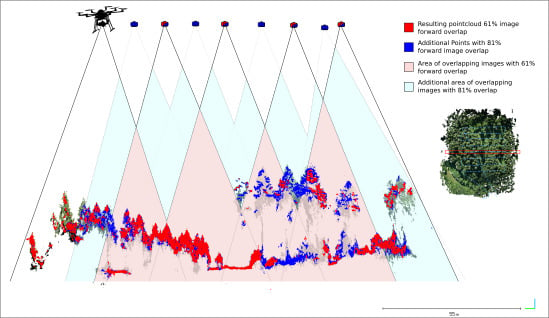
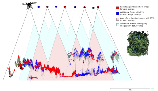
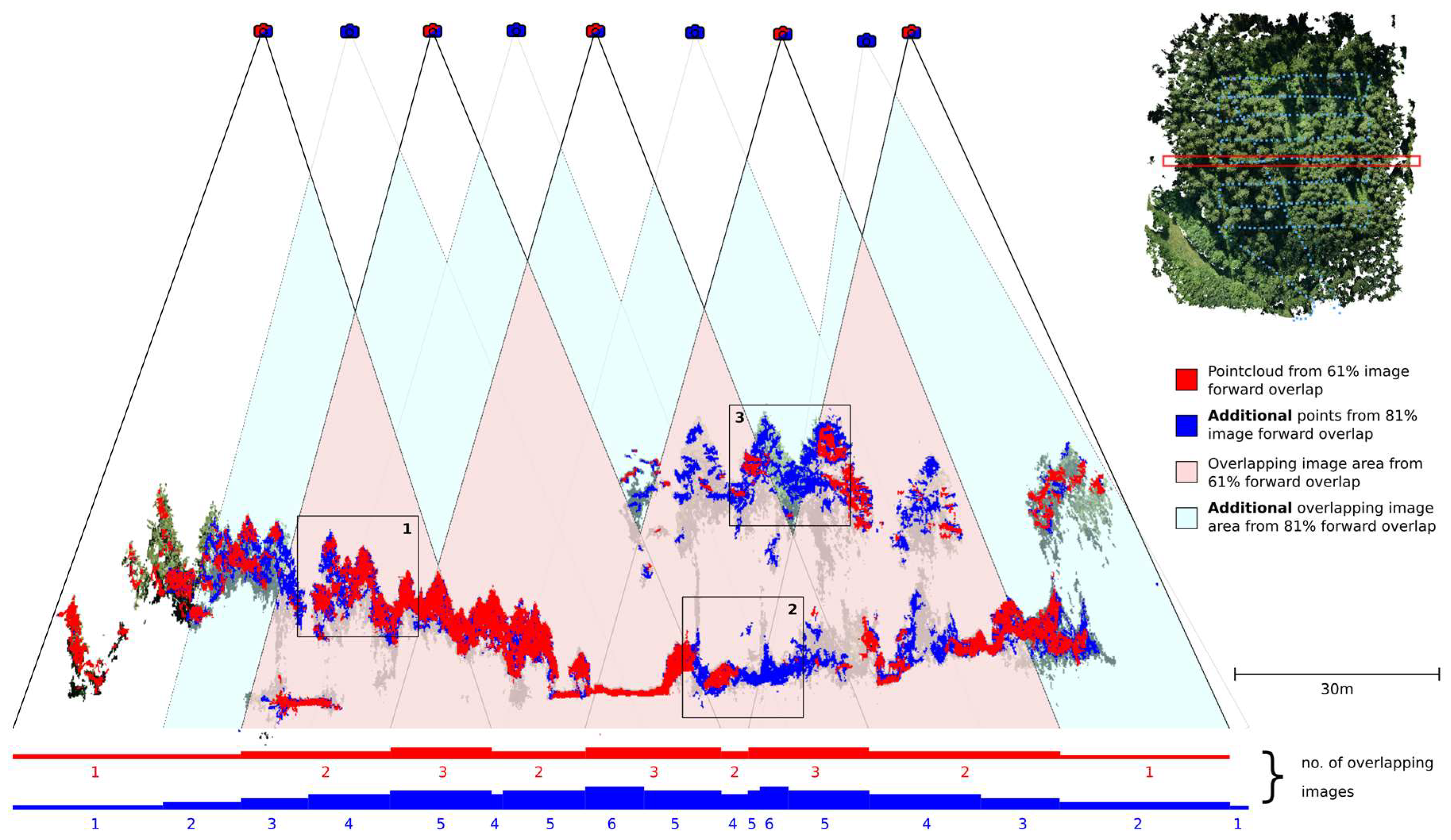
Figure 1 illustrates how doubling the number of images increases the likelihood matching points will be mapped by SfM. This is the result of more perspectives increasing the probability of having a specific feature appear in multiple images, in addition to increasing the amount of sampled vertical space.
Dandois et al. [
18] previously evaluated flight height and image overlap for the reconstruction of tree heights, canopy penetration, and point cloud density. One complicating factor in that study was that both altitude and GSD were varied simultaneously by varying the flight elevation in different scenarios. This created confounding effects on reconstruction completeness and canopy detail that cannot be independently disentangled. Furthermore, the requirement to map structures other than tree height as canopy gaps may differ given that occlusion effects play only a minor role in top of canopy sampling. Consequently, the results of that study are not generalizable for other structural parameters, granted, one of the most important findings is that side overlap of the images plays only a minor role in reconstruction quality.
A study by Torre-Sánchez et al. [
19] optimized the forward image overlap for tree crown volume estimates in olive orchards and outlined optimal results at 95% overlap, while also accounting for processing time. For tree height estimation, they reported that 80% image forward overlap may be sufficient. A valuable contribution for agricultural applications, utilizing a single layered target species of structured olive orchards limits the direct application of findings to complex forested systems where understory vegetation is frequently of interest.
We will measure the quality of forest model output by their completeness in 2D and 3D space. The goal is to generate more broadly applicable results for describing the qualitative aspects of geometric forest representation in models, importantly going beyond single structural parameters of previous works to incorporate a more complete understanding of what contributes to model quality. Overall, we expect a saturation effect according to the image overlap, since additional images will add diminishing amounts of information to the model. For the GSD, we expect an optimum in reconstruction completeness given that very fine images suffer from little movement of branches, as well as additional features which include less information and a higher confusion rate. In contrast, low resolution covers a larger distance within one pixel, making it extremely difficult to gain information on subpixel elements like small treetops or partly occluded elements. As a result, we expect that neither very fine nor very coarse GSDs lead to a good representation in the Model.
2. Materials and Methods
2.1. Research Area
The study was part of the (Conservation of Forest Biodiversity in Multiple-Use Landscapes of Central Europe) ConFoBi Project which has 135 research plots of one (1) hectare each in the Black Forest region of the state of Baden-Württemberg in south-west Germany. The area is a medium sized mountain range between roughly 250 m above sea level in the Rhine valley and 1493m a.s.l. at the highest peak. The area is primarily covered by forest (69%) and has a long history of forest use. The dominant tree species is the Norwegian Spruce (
Picea abies L.) with an admixture of Silver Fir (
Abies alba Mill.) and Scots Pine
(Pinus sylvestris). We find the aforementioned softwood species in 82% of this area’s forest stands, while broadleaf tree species account for less than 30% [
2]. The area is mostly managed using selective harvesting, since clear cuts are strictly regulated in Germany.
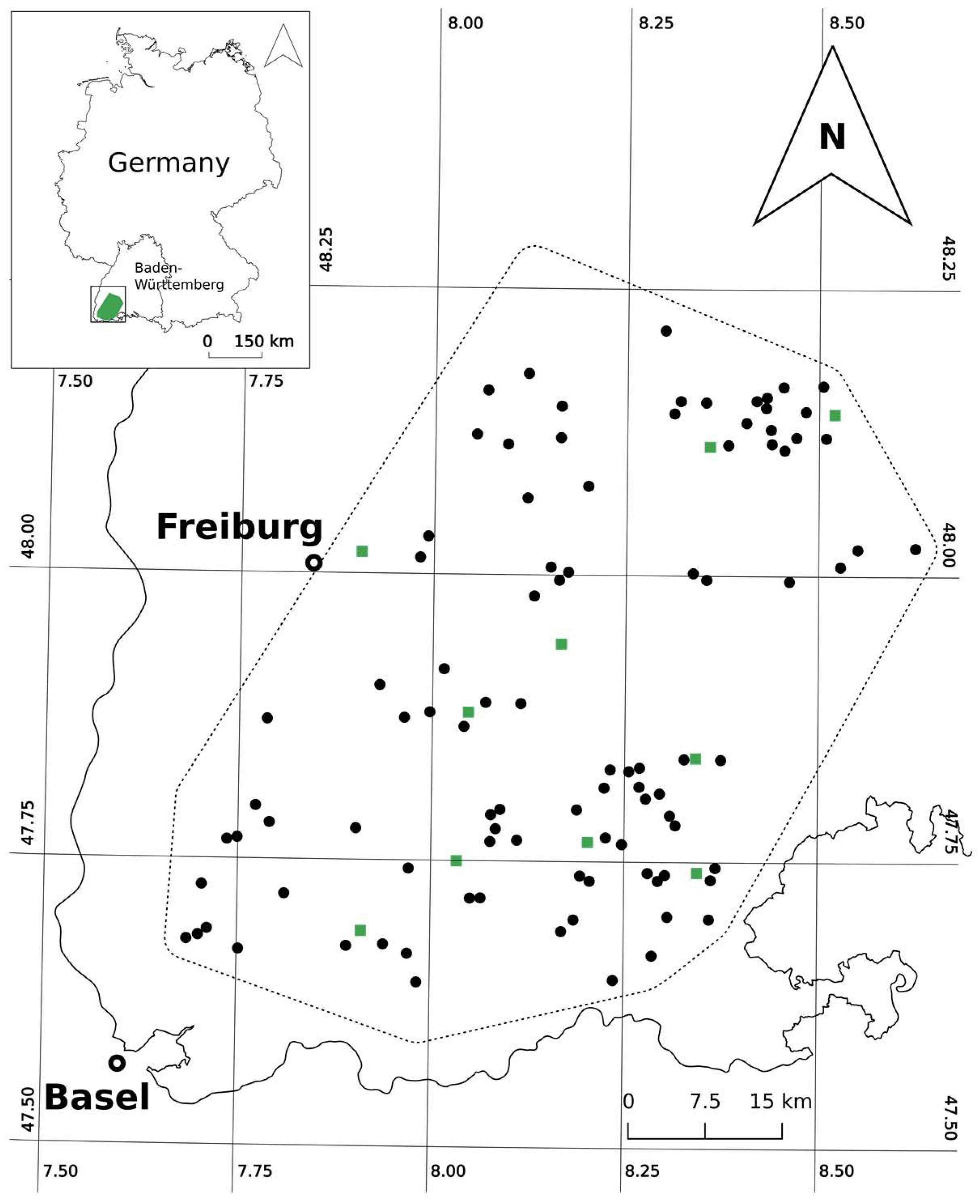
Most (120) of the ConFoBi study plots were covered by UAV-flights during a field campaign in summer and autumn 2017. From these we randomly selected 10 plots (see
Figure 2) for our experiment since the SfM-pipeline is computationally intensive and analysis of the full dataset in all scenarios was not possible.
The resulting plots cover an altitude range of 512 to 1126m a.s.l. with slopes ranging from 8° to 31°. Eight of the plots are managed forest without protection status, two are in bird protection areas, and one is additionally within an EU FFH-nature-protection zone. The plots cover a wide range of forest types and age classes and include some path and skid trails. However roads, waterbodies and anthropogenic structures were excluded by design. The results of the study should therefore be valid over a wide range of forest types and management regimes.
Table 1 provides metrics on the 10 sampled plots.
2.2. Platform, Sensor and Image Aquisition
The aircraft used in this field campaign is an OktoXL 6S12 from Mikrokopter (Mikrokopter GmbH, Moormerland, Germany). A Sony Alpha 7R (Sony Europe Limited, Weybridge, Surrey, UK) full-frame camera with a 35 mm focal length prime lens was used as an RGB camera mounted on an active multi-axis gimbal. The camera was set to F-stop: 2.8, Shutter: 1/2000 s, and ISO-values that were manually adapted to the given lighting situations between 250 and 1000 ISO. The focus was set manually to roughly 70 m. The camera was aligned vertically (nadir) with the aid of a bubble level, and the top side of the camera was set toward the direction of flight.
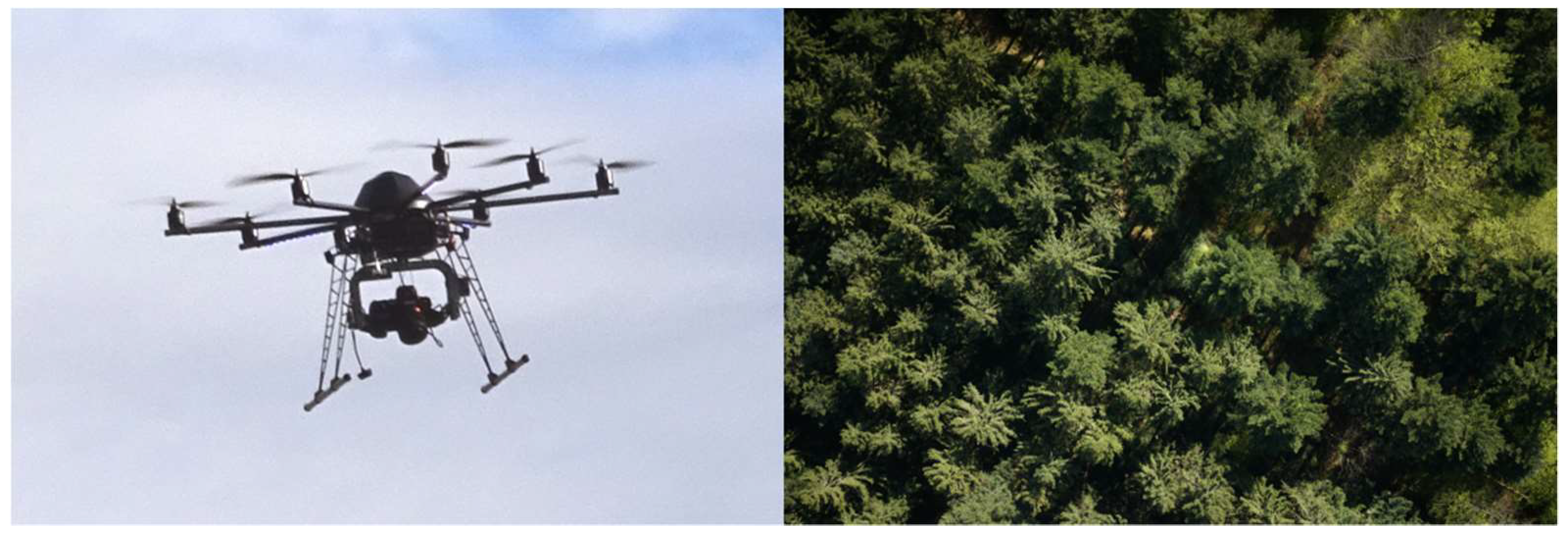
Figure 3 shows an image of the drone platform with mounted gimbal and camera, as well as an aerial image of the canopy taken during flight. The copter was launched manually using a twin stick transmitter and maneuvered through the canopy, after which it was set to autonomous flight according to a predefined flight plan. Following completion of the autonomous mission, manual control was again employed and the aircraft was landed. During the flight, the aircraft automatically triggered the camera every 3 m via a trigger cable, simultaneously recording the GPS position using an internal GNSS sensor (GPS and GLONASS).
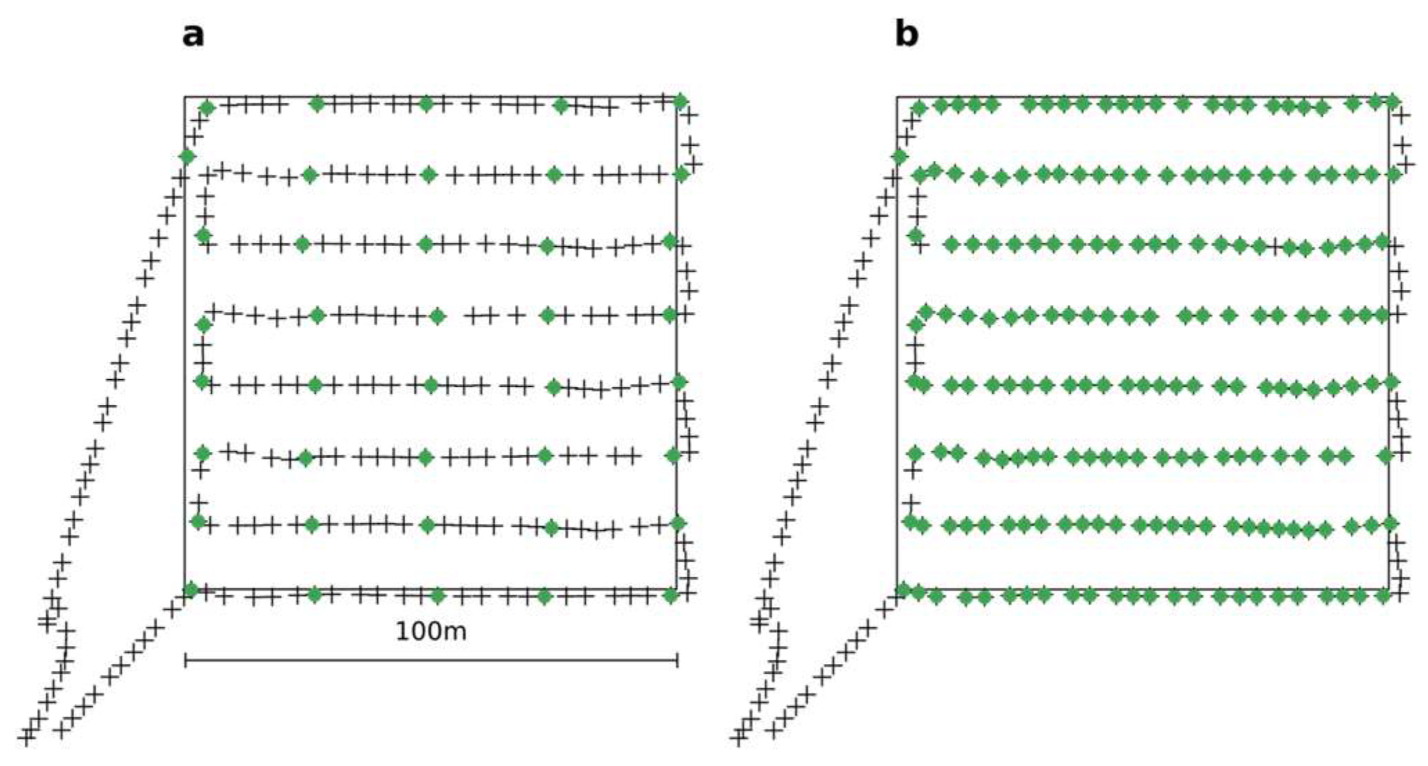
Flight plans were generated preflight using a PostGIS script. Each 100 × 100 m plot was flown in a stripe pattern of seven 100 m stripes buffered by 12.5 m between each. The height was adapted to 80 m above the actual terrain resulting in an 85% sideward overlap (see
Figure 4 for the resulting flight pattern). Since all plots are northerly orientated, we chose to turn the pattern 90° to keep the stripes roughly parallel to the slope. Given that the aircraft only maneuvers according to its relative height to the starting point, we planned flights to start at the lowest point of the plot, thus avoiding collisions with trees in steep terrain. Thus, the starting point defined in the preflight plan was not always utilized given on-site assessments of feasible launch locations. Consequently, flight heights were roughly stable within plots but occasionally varied between plots, with this variance equating to between 72 and 136 m over all sites and resulting in sideward overlap between 83% and 91%.
2.3. Virtual Flight Plans and Down Sampling
Our first plan was to lower the forward overlap between images as employed in Torres-Sánchez et al. [
19]. There the number of images was simply reduced by a thinning approach where every n
th picture was used. This, however, led to artifacts in our study scene since some patterns triggered by this approach led to improved side overlap. Specifically, taking every 10th image led to a line of images along the center of the plot with relatively good results, while taking every 8th image completely failed even if the forward overlap was increased. We therefore calculated multiple realistic flight plans taking 3, 5, 9, 17 and 25 equally distributed images per every 100m stripe, and then choosing the photos that were taken closest in proximity to the planned acquisition point using the UAV onboard GPS for image position.
This led to relatively realistic acquisition scenarios while allowing single flight images to utilize comparable lighting and weather situations. The virtual flight plans were generated and related to the images using R statistical software (Microsoft R Open 3.4.0) [
20]. Afterwards, the respective images not belonging to a virtual flight plan were disabled in Agisoft PhotoScan [
21] (Agisoft LLC, St. Petersburg, Russia) using a Python script.
To verify the influence of the GSD, we used the down sampling option for the raw images available in the “dense point cloud reconstruction” module in PhotoScan [
21]. Selecting the ‘high’, ‘medium’, ‘low’ or ‘very low’ options resulted in 1/4, 1/16, 1/64, or 1/256 of the original pixels by doubling the GSD with every step. Ultimately, calculating the models in original resolution was not possible due to time or computing constraints.
2.4. Point Cloud and DSM Generation
All point cloud and DSM calculations were done in PhotoScan (v. 1.3.4), since this software tends to be the most popular choice among the previously mentioned case studies. We calculated two independent datasets. One, which included 105 flights during the project, used a fixed set of reconstruction parameters and all available images. It was defined as the ‘full dataset’. The second, called the ‘experimental dataset’, included just the 10 random plots as described in the ‘research area’ section. This dataset included all possible overlap and GSD combinations as described in the above section.
For both datasets, the images were referenced by latitude, longitude, and altitude using the GNSS log of the UAV. Thereafter, they were ‘aligned’ (accuracy = high, generic preselection = no, reference preselection = yes, key point limit = 40,000, tie point limit = 4000, adaptive camera model fitting = yes) using the full image data set. This additionally included images from starting, landing and flights to and from the research area to ensure a closed image path. This could potentially be superior for estimation of the interior camera parameters and positioning. These image positions and camera parameters were used for all further analyzes. The software feature to position the cameras and estimate interior orientation were excluded from this analysis given that it could be achieved by other methods as well. For example, this would include using a calibrated camera to achieve the positioning using an inertial measurement unit and differential GNSS, or potentially by picking reference ground points by hand. For the full datasets, we completed the SfM pipeline using dense reconstruction (medium quality, mild filtering) and DSM generation (interpolation disabled).
For the experimental datasets, virtual flight plans came into play. After the image matching procedure was done and all cameras which were not part of the virtual flight plan scenario were disabled, the dense reconstruction with quality settings at the down sampling level were applied using the ‘mild’ filtering option in accordance with Puliti et al. [
22]. We repeated this procedure for four overlap thinning treatments with four GSD down sampling treatments on ten plots resulting in 160 point-clouds. Digital elevation models were computed on these point clouds using default settings. We exported all results as LAZ-files for the point clouds and 5cm resolution tiff-files for the DSMs, as well as the camera positions and orientations as text files.
2.5. Data Processing and Statistical Analysis
All statistical analyses were done in R statistical software (Microsoft R Open 3.4.0) [
20] with the raster and lidR packages included [
23,
24]. We imported all DSMs and point clouds, and clipped them with the defined plot borders to avoid artifacts at the edges. The measure of completeness for the DSM is trivial since we expect a full surface cover on earth. Therefore, we only calculated the ratio of non-filled pixels to the full pixel count. We choose a voxel approach to analyze the coverage of the pointcloud in 3D space with voxels of a 0.1 m edge length. This method is superior to measurements such as point cloud density, since it takes into account the fact that partial or fully-duplicated points observed from many perspectives do not actually contribute more valuable information.
For the voxels, the task of quantifying the completeness is more complicated since we do not know precisely how many of them could theoretically be filled. We therefore assume that the model with the most filled voxels for one plot in the full dataset or one down sampling level in the experimental dataset is the maximum achievable and calculate the ratio of filled voxels according to it. Indeed, this does not necessarily need to be realistic since our interest is in the relative performance of the models. We employed a LiDAR based digital terrain model with 1m resolution provided by the state agency of spatial information and rural development of Baden-Württemberg (LGL), [
25] and the camera position estimates to sample the flight altitude and calculate image overlap as well as the GSD. For the full dataset, further modelling parameters were included such as the altitude of the plot extracted from the DTM, the sun angle calculated from the time of flight, the location, slope and aspect ratio using the model of the sun’s angular position included in the R oce package [
26], and the methodology provided by Mamassis et. al. [
27] to compute the sun’s direct radiation on the topography. The average hourly wind speed at the time of flight retrieved from a weather station of the German weather service at the Feldberg Mountain (central high peak in the research area) was taken into account as well to distinguish between more or less windy days within the region.
All model parameters were tested for collinearity visually using a correlation plot. For the full dataset, GSD and overlap are correlated, which was expected given their lack of independence in this setting. Respectively, GSD was dismissed as a predictor variable for the full dataset. Furthermore, the overlap variable of this model represents the effect of the GSD. The resulting model formulas for the experimental dataset were:
and for the full dataset:
3. Results and Discussion
The visual interpretation of pointclouds from different overlap scenarios revealed major differences in reconstruction quality (
Figure 1,
Figure 5b and
Figure 6). While most of the upper canopy reconstructed well in all overlap scenarios as long as the overlap was sufficient (
Figure 1: box 1), parts of the understory and ground suffer at lower overlaps from strong occlusion effects (
Figure 1: box 2).
Figure 1: box 3 highlights that while ground based overlap may be sufficient given higher flight elevation, it may already be too low for large top of canopy trees.
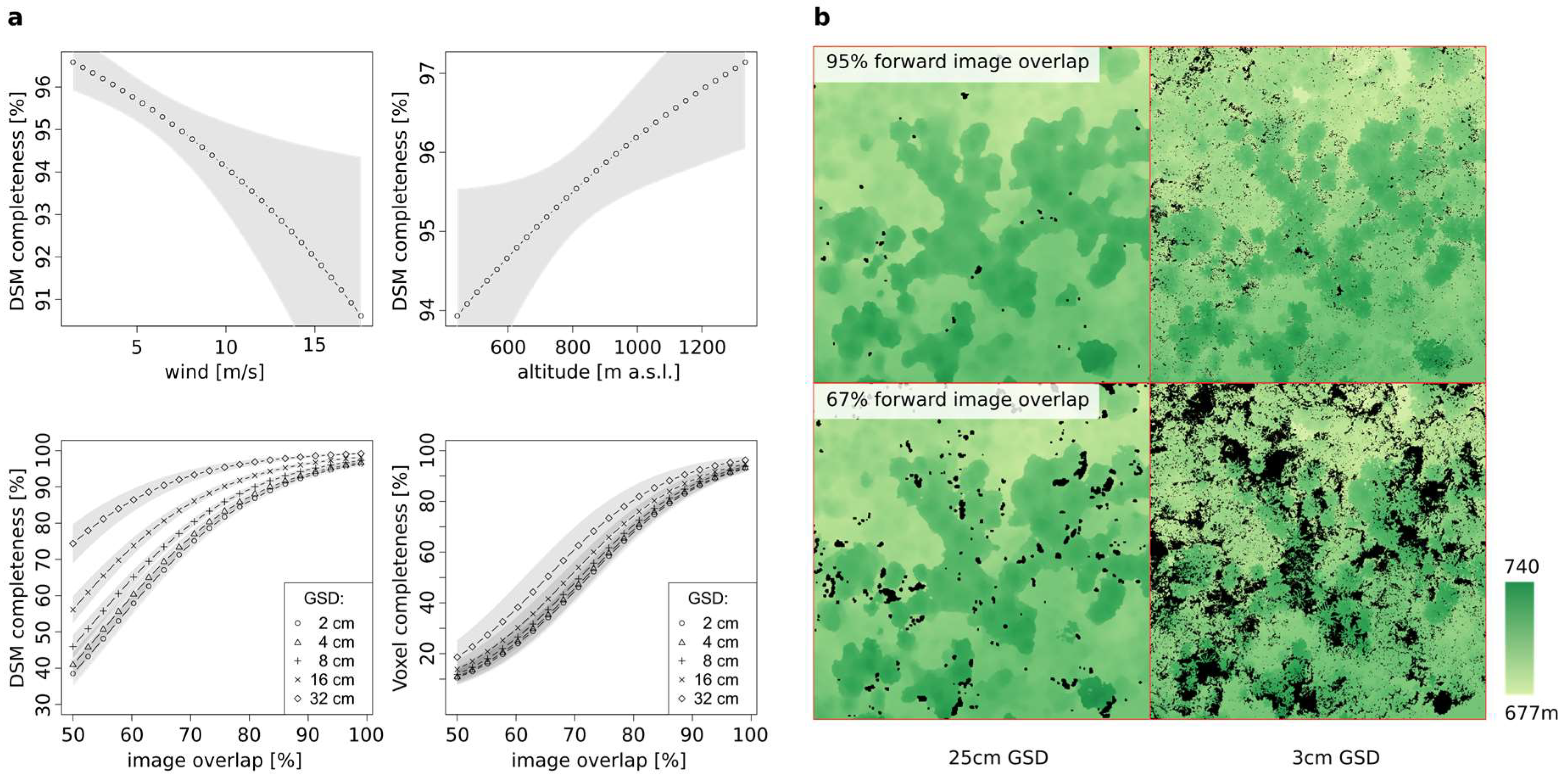
Statistics carried out on the experimental dataset showed a clear positive correlation between GSD image overlap and the model completeness in both 2D and 3D (all
p-values: < 0.01).
Figure 5 shows the effect plots including the 95% confidence intervals. Based on our results, the effect of the image overlap is far more important than the effect of the GSD. This is especially relevant when taking into account, for most applications, a fine GSD can be beneficial, while a high image overlap is relatively easy to achieve. With an image forward overlap of >95%, even at GSDs of 2 cm, a DSM-completeness of 95% is possible, while common lower overlaps of ≤80% ([
3,
4,
10,
11]) require a GSD >20 cm to reach equivalent spatial coverage.
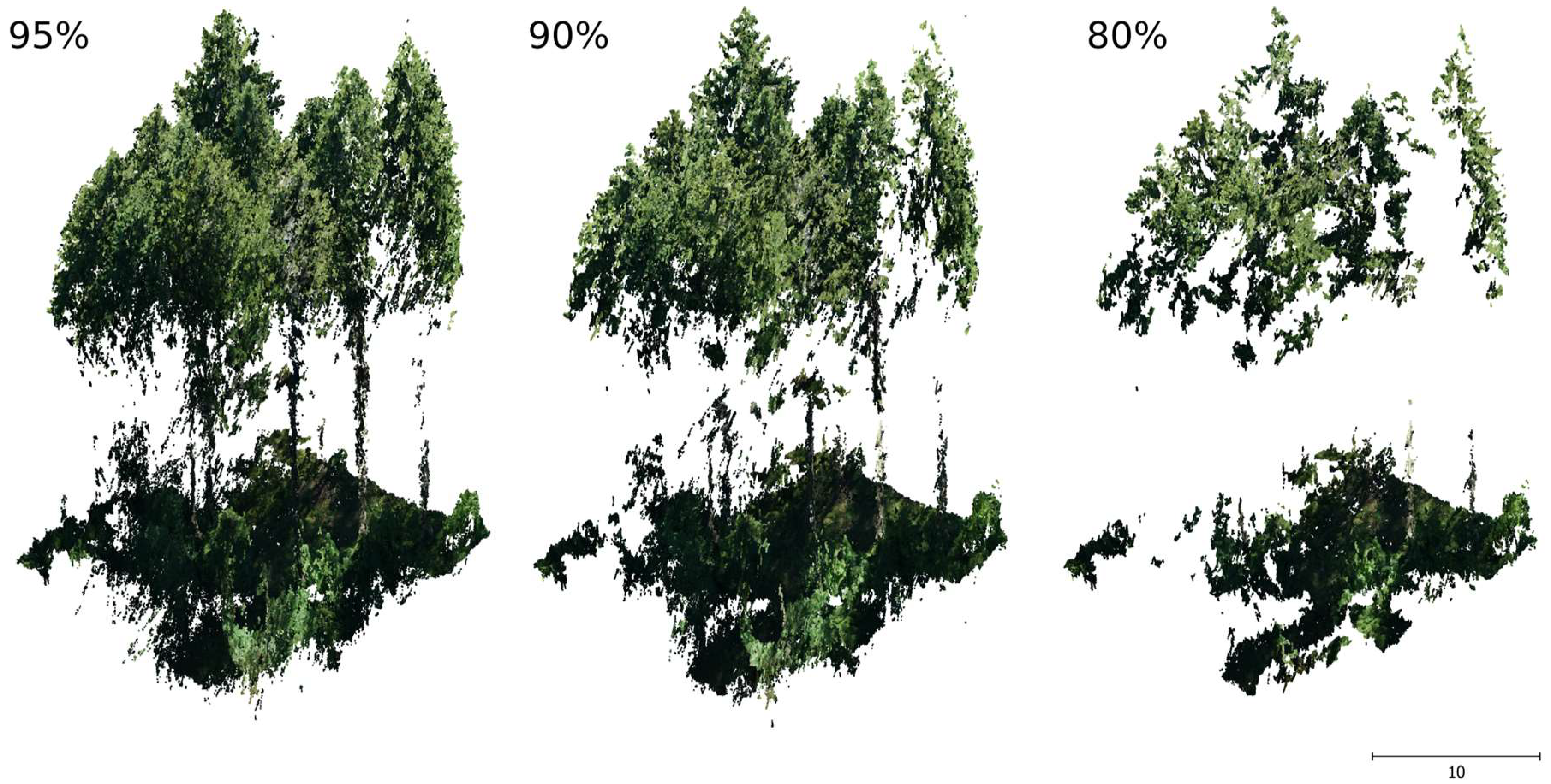
Figure 6 presents the 3D point clouds with varying degrees of overlap. While the most elevated points are reconstructed almost independently of the overlap, actual point density decreases sharply as overlap decreases. The DSMs in
Figure 5b visually convey the results, however it is not clear why a higher GSD is favorable for reconstruction. Possible explanations could be that a higher GSD avoids wind effects on scene elements that could cause a change between pixels, and that slightly larger elements may be more easily identified by the algorithm if the perspective changes.
These results are in line with Torres-Sánchez et al. [
19] and Dandois et al. [
18] according to the level of image overlap. In those studies, however, GSD and image forward overlap were never independently assessed as contributing to reconstruction quality. A mechanistic assessment of the independent contribution of these two variables is a key result of this study.
Cunliffe et al. [
28] showed that very fine GSD (0.004–0.007 m) DSMs can be generated with high precision, particularly by including the addition of 45° camera angle photos. This study was conducted on drylands (mostly shrub and grassland vegetation), with a single fixed forward image overlap of 70%. The application of this methodology to more geometrically complex multilayered environments remains a question for further research. However, Fritz et al. [
7] has shown that 45° images are useful for diameter at breast height estimates in oak forests during leaf-off conditions, suggesting a limitation in its usefulness in coniferous stands, or during leaf-on.
The sensitivity of the model completeness to image overlap was even stronger in 3D than in 2D, while the advantages of lower GSD vanished in voxel space. This strongly suggests that a finer GSD and high image overlap are both beneficial for sampling lower parts of the canopy, understory, and ground. Nevertheless, visual interpretation of the DSMs revealed that reconstruction of the stands with lower canopy height (regrowth stands and patches) exhibited better performance, potentially a direct effect of the higher sampling distance at top of the canopy, as well as the higher overlap (
Figure 1). This leads to the conclusion that flight elevation should be adapted to the target stand height.
Analysis using the full dataset revealed that wind contributed as a major influencing factor (
p-value < 0.01), which is not surprising given tree movement is a significant barrier to the matching and reconstruction workflow. Dandois et al. [
18] additionally highlighted that wind was the major influencing factor for UAV turbulence during flights, resulting in varying acquisition distance and angles, and thus leading to heterogeneous image overlap. We see two possible solutions to overcome this problem. The first is to limit flights to windless conditions, and the second is to take all pictures simultaneously utilizing swarm robotics. Indeed, this might not be suitable given our results covering image overlap presented above. Moreover, increasing the GSD also minimizes the wind effect, since tree movement becomes minor in relation to the pixel size.
There was also a positive effect of terrain altitude on reconstruction completeness (
p-value: 0.02), which is more challenging to decipher. A possible explanation could be vegetation variation across elevation gradients, with generally lower tree heights and more sparse vegetation in higher elevations. More research would be required to explain this phenomenon. Terrain slope (
p-value: 0.53), aspect (
p-value: 0.09), and the relative angle of the sun at plot surface were not significant (
p-value: 0.83). This finding is surprising given that various authors attribute shadows to issues in the reconstruction pipeline ([
4,
5,
10,
15,
18]). The vulnerability of the process to lighting conditions may also be directly linked to the quality of the sensor and its spectral bands. Other spectral information on vegetation may exhibit stronger variance according to lighting conditions than in the visible bands. O’Conner et al. [
29] gave a good overview of lens and camera setups and their ability to acquire images with sufficient spectral information, low distortion, and blur. Given that only one sensor and lens combination was used, this question may also benefit from further research.
4. Conclusions
There is a clear and quantifiable relationship between image forward overlap, GSD, and the completeness of the model reconstructed using a structure from motion pipeline. The quality of the information acquired by employing such a model is important to proper flight parameter choice and adjustment for environmental conditions. This requires a clear, outlined methodology concerning the decisions made during the planning phase for UAV based studies to avoid misinterpretation. The tradeoff between flight effort, precision (coarse GSD), and model completeness must be balanced carefully according to the specific goals of the study. Moreover, since full coverage is difficult to achieve when utilizing SfM-based datasets, the proportion of area not covered as a part of the whole should be reported.
Our interpretation of SfM rendered point clouds revealed a relatively high number of ground points which challenge the idea that only LiDAR derived DTMs are valuable in mapping forest structure (
Figure 6). This is not surprising given that ground and lower canopy structure suffer more from the effects of occlusion. A high image overlap in combination with a fine GSD requires increased resource planning, but may be key to extract enough ground points to accurately reconstruct the terrain. Further research in this field is required to adapt existing algorithms used for LiDAR-DTM reconstruction to SfM-pointclouds and its outliers such as below ground artifacts. Thus, this has the potential to increase usability of SfM data for forest applications, especially in regions where LiDAR-DTMs are unavailable.
In summary, UAV-based SfM remains a promising technique for forest structure mapping, and we hope this sets a basis for future evidence based flight planning.


