Quantitative Estimation of Wheat Phenotyping Traits Using Ground and Aerial Imagery

Abstract

This study evaluates an aerial and ground imaging platform for assessment of canopy development in a wheat field. The dependence of two canopy traits, height and vigour, on fertilizer treatment was observed in a field trial comprised of ten varieties of spring wheat. A custom-built mobile ground platform (MGP) and an unmanned aerial vehicle (UAV) were deployed at the experimental site for standard red, green and blue (RGB) image collection on five occasions. Meanwhile, reference field measurements of canopy height and vigour were manually recorded during the growing season. Canopy level estimates of height and vigour for each variety and treatment were computed by image analysis. The agreement between estimates from each platform and reference measurements was statistically analysed. Estimates of canopy height derived from MGP imagery were more accurate (RMSE = 3.95 cm, R${}^2$ = 0.94) than estimates derived from UAV imagery (RMSE = 6.64 cm, R${}^2$ = 0.85). In contrast, vigour was better estimated using the UAV imagery (RMSE = 0.057, R${}^2$ = 0.57), compared to MGP imagery (RMSE = 0.063, R${}^2$ = 0.42), albeit with a significant fixed and proportional bias. The ability of the platforms to capture differential development of traits as a function of fertilizer treatment was also investigated. Both imaging methodologies observed a higher median canopy height of treated plots compared with untreated plots throughout the season, and a greater median vigour of treated plots compared with untreated plots exhibited in the early growth stages. While the UAV imaging provides a high-throughput method for canopy-level trait determination, the MGP imaging captures subtle canopy structures, potentially useful for fine-grained analyses of plants.

1. Introduction

Plant development is observable as changes in a plant’s morphological features, which occur at specific growth stages. For example, plant development may result in the appearance of new features such as reproductive organs (i.e., flowers) or a change in the pigmentation of the plant foliage. Plant growth is not only characterized by an increase in the size of existing plant organs (elongation and thickness of stems and area of leaves), but also by the emergence of new shoots of a similar morphological feature (new leaves, new stems), which contribute to the overall increase in plant vegetative volume [1]. The underlying ability of a plant to grow and develop, steered by the environment, results in a phenotype that can be traced back to its genotype. One aim of a plant phenotyping exercise is to characterize and quantify the relationship between the genotype and the phenotype as a function of environmental conditions.

Classical phenotyping relies on manual sampling and trait analysis of developing plants to characterize a plant’s growth and development. This process requires a significant amount of time and resources. While demanding, manual inspection of plants is feasible on a small scale and under controlled conditions. However, sampling of plants in a field setting, which usually involves an enormous number of plant varieties and is subject to significant variations in environmental conditions (as arise in practical circumstances such as in plant breeding trials), represents an overwhelming prospect.

Novel image analysis systems are now being designed and implemented to automatically capture the ensuing morphometric changes in plant traits in the field [2]. State of the art imaging hardware and image analysis methods have attracted considerable interest from the plant phenotyping community. This is not only due to their potential of relieving the burden of manual phenotyping, but also the possibility of objectively quantifying trait characteristics [3]. Land-based phenotyping platforms, such as the mobile ground platform (MGP) used in this study, are able to capture high resolution images of plant canopies at close range. The corresponding image analysis software is rapidly becoming available and reliable [4,5,6]. In comparison, aerial imaging platforms such as an unmanned aerial vehicle (UAV), have recently found application in field phenotyping [7,8]. The main advantage of a UAV is that it can cover larger areas, thus offering high-throughput field capture, albeit with a trade-off of resolution. Consequently, these platforms are utilized for the assessment of nurseries and breeder plots [9]. The plot-wise characteristics that are usually targeted for capture are canopy vigour [10,11], canopy height [12], biomass [13], leaf area [14] or ground cover [15].

Canopy height, defined as the distance between the base of a plant and the highest photosynthetic tissue, is a gross, but important indicator of a plant’s physical development. Measurement of plant height using a ruler has long been the traditional approach [12,16,17]. Assessment of plant height from images is a far more complex process as it necessitates the estimation of depth in physical units; in discipline terms, a so-called depth map is reconstructed from multiple images of a canopy taken from slightly different viewpoints. Relevant work in this area has shown that accurate estimates are possible and indeed preferable given their objectivity and accuracy, compared with manual measurements, which can be subjective, as well as incomplete [5]. An alternative method, light detection and ranging (LiDAR), uses an active laser sensor to non-destructively measure canopy height with high accuracy [17].

The second readily-identifiable trait that communicates plant status at a given stage of development is canopy vigour. Typically, the physicochemical state of leaf and stem pigmentation and the density of foliage are major factors that contribute to canopy vigour [10,18]. Indirectly, vigour can be quantified in terms of a vegetation index (VI), which involves a plant’s calibrated reflectance at different wavelengths. A vegetation index can be used as a non-destructive substitute of vigour, assuming it is proportionally related. Although there are some exceptions [19], vegetation indices are most commonly defined as ratios of differences to sums of reflectance in two or more bands. For example, the commonly-used normalized difference vegetation index (NDVI) is a ratio of the difference between the plant’s reflectance in the near-infrared and red bands to the sum of the reflectance [20,21,22]. While manual hand-held sensors with infrared capabilities have been used to measure the reflectance and compute indices on a small scale, high-throughput imaging techniques are preferable for large-scale studies.

Vegetation indices that can be derived from RGB images [23] include the excess green index (ExG) [24], the modified hue index [25], which applies the inverse cosine function to a combination of the red, green and blue (RGB) values, and the green-red vegetation index (GRVI) [26], defined as the ratio of the difference to the sum of plant reflectance in the green and red channels. Kipp et al. found the relative amount of green pixels (RAGP) index to be proportional to plant vigour [10]. A recent study showed that a number of VIs, including ExG and NDVI, did not significantly differ in the ability to assess plant vigour [27]. In this study, GRVI has been used to represent and proportionally quantify plant vigour. The index normalizes for variations in light intensities, has been a tested indicator of chlorophyll content in several crops and is shown to be positively correlated with traits such as biomass [28] and leaf area index [29], a quantity related to plant vigour. In this study, images of plant canopies are captured in the RGB channels, making an RGB-derived index suitable to represent vigour by both MGP and UAV. While acknowledging that several different indices can be derived from an RGB image, the rationale for choosing a single index is to compare the attributes of MGP and UAV image-based estimates of vigour on the same scale.

Close-range images of the field are captured with sensors attached to ground vehicles [6,30,31,32,33] or mobile platforms [5,34,35] for trait estimation. On the other hand, remote images of the field are captured with sensors attached to aerial platforms [36,37,38,39] for trait estimation. Recent studies to quantify plant canopy development from images either report trait comparisons with reference to a different sensor technology such as LiDAR [16,40] or compare image-based estimation techniques with manual methods [5,41]. A comparison of the performance of two imaging methods on the same field study has hitherto not been reported previously. In this paper, we provide such analysis for quantitative estimation of phenotyping traits of wheat in a field trial. Our comparative analysis is both relative and absolute since we have also employed the results of traditional manual methods of measurement as a benchmark for the MGP and UAV imaging. The analysis is focused on canopy height and vigour, which are two important plant phenotyping measures.

2. Materials and Methods

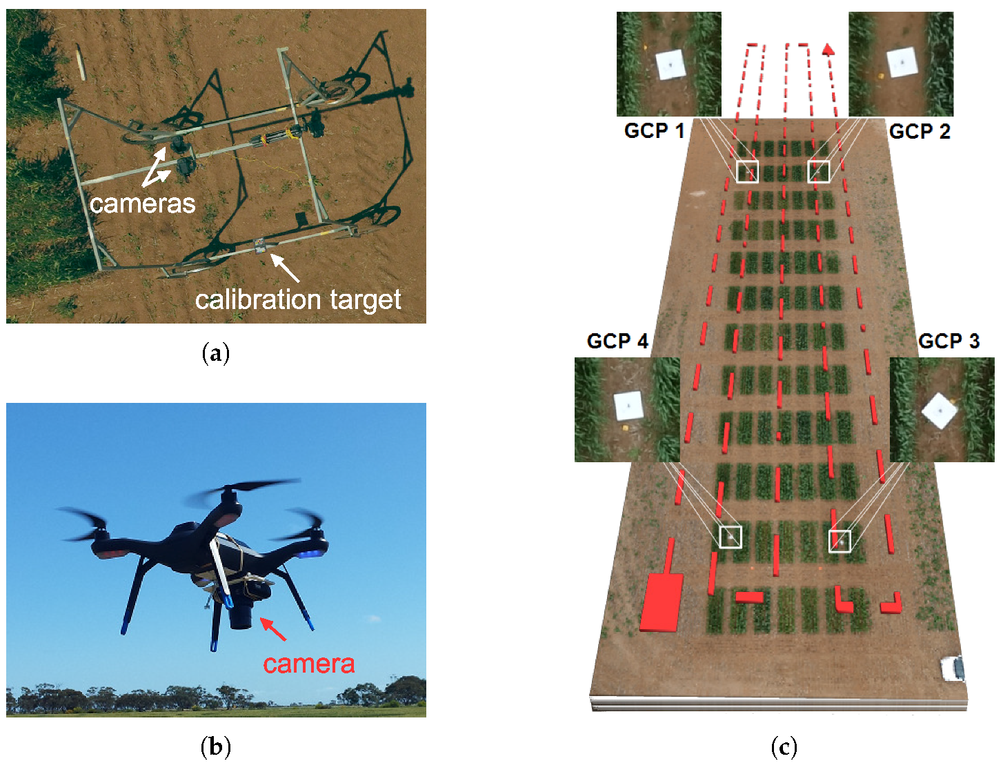
2.1. Experimental Design

A field trial to observe the differential growth of wheat with fertilizer treatment was conducted at Mallala, South Australia (latitude = $-{34.457062}^{\circ }$ , longitude = ${138.481487}^{\circ }$). A set of ten contrasting varieties (Drysdale, Excalibur, Gladius, Gregory, Kukri, Mace, Magenta, RAC875, Scout, Spitfire) of spring wheat (Triticum aestivum L.) were selected for the experiment to cover a diverse range of growth characteristics. Six replicates of each variety were laid out in a 5 × 12 randomized split-block design of 60 plots, as shown in

Table 1. Randomized split-block design layout of thrice replicated wheat varieties, Vn, n $\in \{1,\dots ,10\}$. Shaded blocks were treated with fertilizer.

	Col	1	2	3	4	5	Rep
Row
1		V3	V6	V10	V4	V7	1
2		V8	V2	V5	V1	V9
3		V2	V5	V1	V9	V8
4		V7	V4	V6	V3	V10
5		V9	V1	V10	V6	V8	2
6		V7	V3	V4	V5	V2
7		V3	V7	V5	V4	V6
8		V9	V10	V2	V8	V1
9		V2	V3	V1	V10	V5	3
10		V6	V8	V7	V4	V9
11		V8	V7	V10	V1	V4
12		V6	V5	V3	V9	V2

. Additional plots, not included in the trial, were added to either end of the rows to attenuate edge effects on the border plots.

The trial was sown on 8 July 2016 at a seeding rate of 45 g per plot. The plot dimensions were 1.2 m × 4 m, containing 6 rows of wheat with an inter-row spacing of 0.2 m. Three replicates of each variety were selected for fertilizer application. A top dressing of a standard mix of 16:8:16 N-P${}_2$O${}_5$-K${}_2$O was applied 35 days after sowing at a rate of 37.5 g m${}^{-2}$. A following top dressing of urea was applied 62 days after sowing at a rate of 4.3 g m${}^{-2}$. The remaining three replicates of each variety served as controls and received no fertilizer treatment.

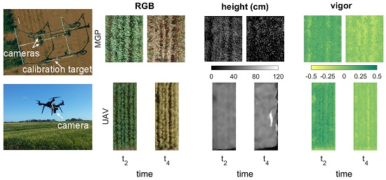
2.2. Image Data Collection and Analysis

Comparative data collection was performed five times between August and November of 2016 (see

Table 2. The phenological development stage (BBCH-scale) of wheat and the respective days on which images and reference data were collected. I: interpolated, A: actual, N: not available.

t	Stage	(BBCH-Code)	MGP Date (Height, Vigour)	UAV Date (Height, Vigour)
1	stem elongation	(34)	23/09/16 (A, I)	19/09/16 (I, A)
2		(37)	07/10/16 (A, A)	07/10/16 (A, A)
3	anthesis	(63)	28/10/16 (A, I)	26/10/16 (I, A)
4	grain development	(77)	08/11/16 (A, I)	09/11/16 (I, A)
5	senescence	(92)	18/11/16 (A, N)	18/11/16 (A, N)

). MGP imaging was conducted following manual measurement of plant heights, whereas UAV imaging was conducted following manual measurement of canopy vigour. For practical reasons (e.g., adverse weather conditions), MGP and UAV could not always be deployed for image collection on the same day. However, imaging sessions differed by at most four days, in most cases fewer (see Table 2). The difference resulted in the unavailability of height reference measurements on some days of UAV imaging and vigour reference measurements on some days of MGP imaging. This limitation was addressed by linearly interpolating reference data taken on days immediately prior to and subsequent to the days of missing data. Such an approach was considered appropriate for the analysis since reference measurements were always available within a range of less than four days.

2.2.1. MGP Imaging and Canopy Trait Estimation

Our MGP imaging system consisted of two identical EOS 60D digital SLR cameras (Canon Inc., Tokyo, Japan) with a resolution of 18.1 megapixels, synchronized to capture images within 1 ms of each other by means of an electronic trigger. The cameras were mounted on a custom-built wagon, 20 cm apart on a central overhead rail, 1.90 m above ground level. The platform was manually driven to a stop at three equidistant positions in each plot to capture images of its entire area. By fixing the camera positions relative to a plot, subsequently captured images of the same plot automatically fell into coarse alignment. Cameras were adjusted to focus at a depth of 2 m in the early growth stages and 1.5 m at later stages to capture sharp images of canopies with growth. The remaining camera settings were as follows: focal length: 18 mm; aperture: f/9.0; ISO: automatic; and exposure: 1/500 s. The arrangement of MGP imaging system is shown in Figure 1a.

A ColorChecker Passport Photo (X-Rite Inc., Grand Rapids, MI, USA) calibration target was used as a basis for colour correction. The calibration target was attached to the base of the platform such that it was always visible from the perspective of one camera as described in Appendix C. Colour calibration was performed on all images according to the method proposed in [41]. Field imaging was carried out between 23 September 2016 and 18 November 2016 inclusive (see Table 2).

The acquired stereo image pairs were processed to reconstruct the depth of the plot canopy. Firstly, the lens distortion was corrected by taking advantage of the calibration images from the locally flat ground (i.e., no additional calibration was applied or indeed needed). A given stereo pair of cameras was positioned with optical axes aligned in one plane. If the lenses of the stereo cameras were undistorted and the plane of the camera sensors was parallel to the ground plane, the distance between any two key points on the flat ground (plane) would be the same in the stereo pair of two images. By taking advantage of this, we can estimate the lens distortion parameters. Then, a pixel-wise matching technique was used to estimate the distance between corresponding points in the image pair [42]. In this approach, the estimation of a depth image relied on reference data in the form of the camera focal length and the physical distance between the two cameras. An approximate ground sampling distance (GSD) of 0.04 cm per pixel was achieved in the processed images. A detailed description of the procedure is provided in [5].

The height distribution of plant tissues within a plot, i.e., the frequency of occurrence of plant material at a given height above ground level was computed from the depth images that were derived using the above-mentioned procedure. A sample graph of the height distribution is provided in Figure A3. Overall canopy height, as presented in the analysis to follow, was defined as the 98th percentile of the canopy height distribution of a plot (refer to Appendix B for details on percentile selection).

Vigour per plant pixel, computed separately from the colour-calibrated images, is defined as the ratio of the difference in plant reflectance in green and red channels to the sum of the reflectance,

$$\mathrm{vigour}\sim GRVI=\frac{\mathrm{Green}-\mathrm{Red}}{\mathrm{Green}+\mathrm{Red}}$$

(1)

The value of this quantity, averaged over the three RGB images per plot, was used as a representative measure of plot canopy vigour.

2.2.2. UAV Imaging and Canopy Trait Estimation

Our UAV imaging system was a 3DR Solo quadcopter (3D Robotics Inc., Berkeley, CA, USA) with a RX100 III Compact Digital Camera (Sony Corp., Japan) as the payload giving an effective image resolution of 20.1 megapixels. Flights were planned using the open source ground control station software, Mission Planner (ArduPilot), which directed the UAV to follow a preprogrammed path based on the geographical coordinates of the site as shown in Figure 1c. The camera was set to automatically capture snapshots every 2 s during flight at an altitude of 30 m, which resulted in an image-overlap of more than $80\%$. Five imaging sessions were conducted from 19 September 2016–18 November 2016, inclusive (see Table 2). A standard reflectance panel (MicaSense Inc., Seattle, WA, USA) was photographed before each flight for radiometric calibration of the images. Colour images were stored as compressed JPEG files.

Inaccuracies in location estimates provided by the GPS receiver onboard the UAV contributed to an uncertainty in the global alignment of orthomosaics captured at different times. To overcome this deficiency, square panels, termed ground control points (GCPs), were used to provide a location reference. A total of four such GCPs were consistently placed at fixed field locations before each imaging session. This facilitated alignment and scaling of the orthomosaics over the whole season.

UAV images acquired in a given session were processed offline using the professional photogrammetry software Pix4Dmapper v4.0 (Pix4D, Lausanne, Switzerland). The processing comprised three main steps for 3D canopy reconstruction using the structure from motion (SfM) technique [43]. Initially, ‘keypoints’ were automatically computed from original images. Keypoints refer to visual features of interest that can be detected reliably in images taken from different perspectives. These points were matched across all the images to estimate camera position, orientation and internal camera parameters. The original images were corrected for any lens distortion using a camera calibration model [44]. In the second step, matched keypoints were triangulated to create a dense three-dimensional point cloud. In the final step, the following raster images were output as TIFF files:

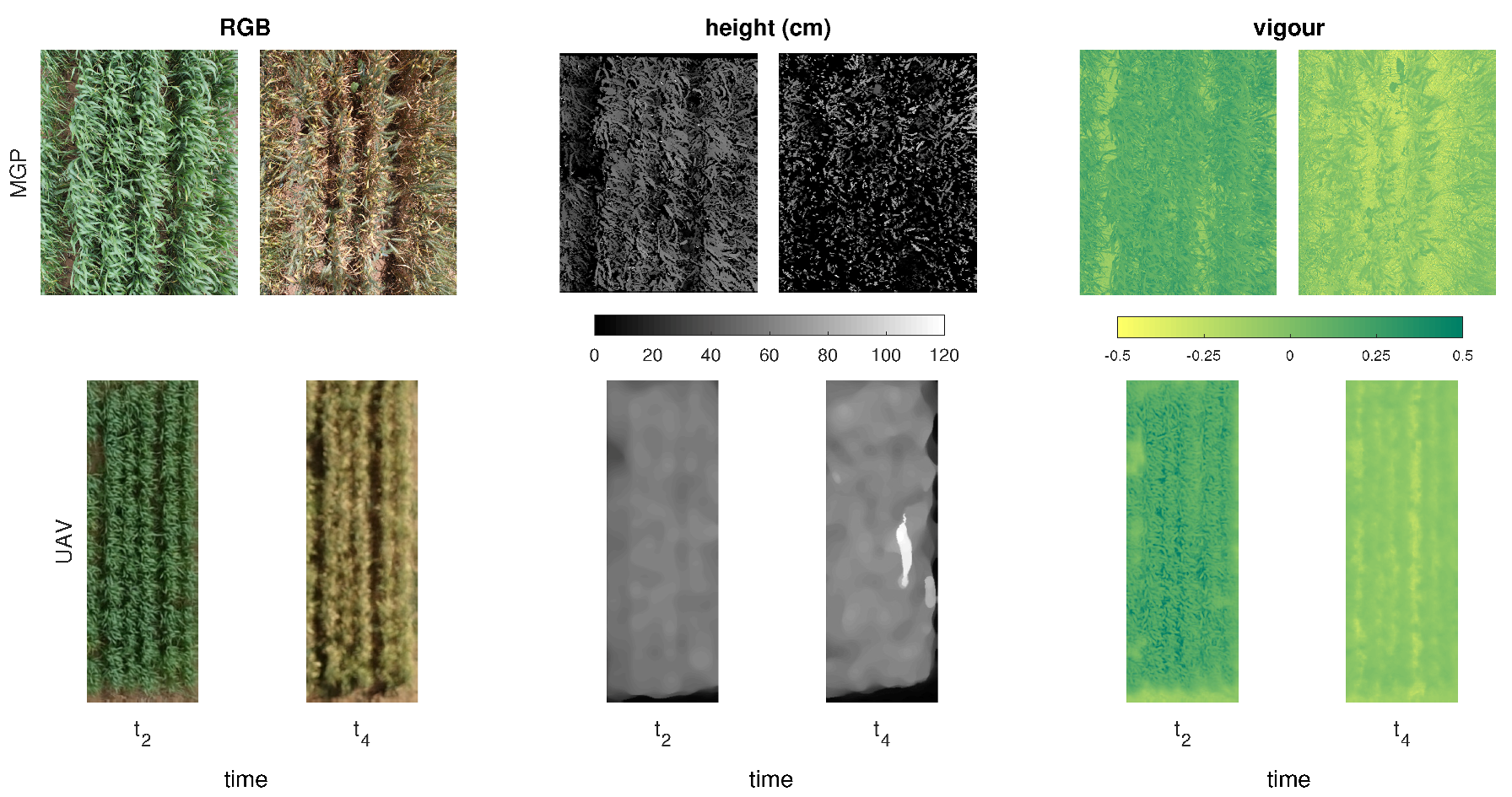
• Height map (also known as a digital surface model): Elevation (in cm) of the mapped surface generated by interpolating the point cloud.
• Terrain map (also known as a digital terrain model): Elevation (in cm) of the mapped terrain excluding any above-ground features (e.g., plants). This output was visually assessed and confirmed to have filtered out the plants within each plot.
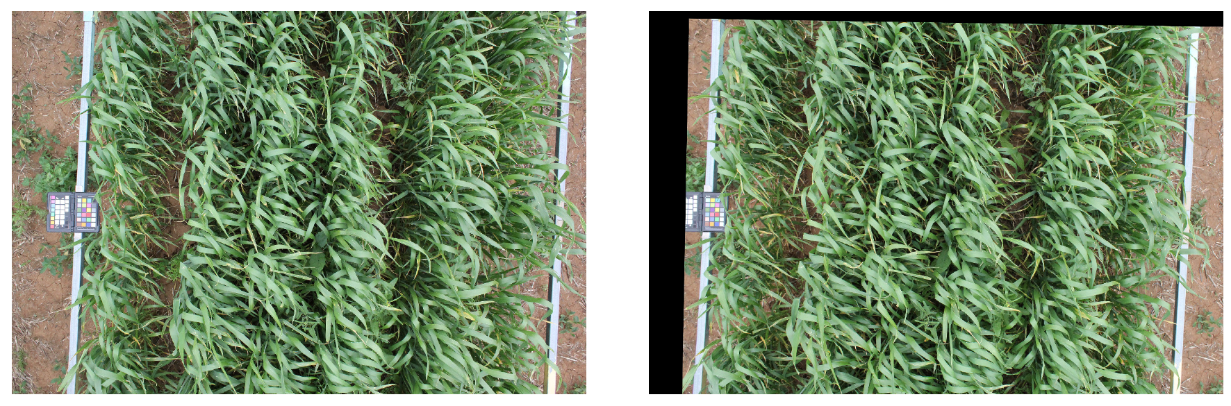
• Reflectance map: A colour-calibrated image generated by projecting ortho-rectified images onto the height map. This output is colour calibrated using pixel values of the radiometric calibration target.

The output images resulted in an average GSD of 0.8 cm. The software uses manually-marked locations of each GCP in six to eight images in order to register (position and scale) the output images at different times. Spatial analysis of the trial was performed by importing the reflectance, height and terrain images into MATLAB R2017b (Mathworks Inc., Natick, MA, USA). A rectangular lattice, sized and spaced according to the plot dimensions, was interactively overlaid on the reflectance image to establish the region of interest. The height distribution within the bounds of the region of interest of a plot relative to the ground, was computed by subtracting the terrain map from the height map. The canopy height was designated as the 98th percentile of a plot’s height distribution. Vigour, defined by Equation (1), was computed per pixel within the region of interest from the reflectance map. The average of this quantity taken over all plot pixels was used as a representative of plot canopy vigour.

2.2.3. Ground Reference of Canopy Traits

A total of 300 height observations were recorded for the 60 plots on five occasions during the growing season concurrent with the MGP imaging days (see Table 2). Canopy height was manually measured using a meter rule with markings every cm. A measurement was taken by placing the ruler vertically inside a plot and reading the ruler at the top of the canopy. Multiple locations within each plot were sampled and averaged to get a single representative measure of the canopy height of a plot. During the early stages of plant growth, when spikes were not present, canopy height measurement related to the leaves only. Later, when flag leaves and spikes appeared, these features were also included in the measurements. That is, plant height was defined (and recorded) to be at the top of the level of the spike layer; awns, if any were present, were excluded from the measurements.

A total of 240 vigour observations were recorded for the 60 plots on four occasions during the growing season concurrent with the UAV imaging days (Table 2). A GreenSeeker hand-held crop sensor (Trimble Inc., Sunnyvale, CA, USA) was used to record the reference measure of canopy vigour. GreenSeeker is an active optical sensor that quantifies plant vigour using the NDVI ratio, (NIR − red)/(NIR + red). A continuous longitudinal sweep of the sensor at a constant height above a plot gave a representative measure of canopy vigour. The theoretical range of sensor measurement was (0.00–0.99); a higher value indicated greater vigour, and a lower value indicated less vigour. The observed range of reference canopy vigour of wheat plants in this trial was found to be (0.30–0.80). Although we have shown elsewhere that NDVI can be closely estimated by RGB images [45], it is inherently different from the GRVI derived from RGB images reported in this study. This difference must be borne in mind in the comparison that follows.

2.3. Statistical Analysis

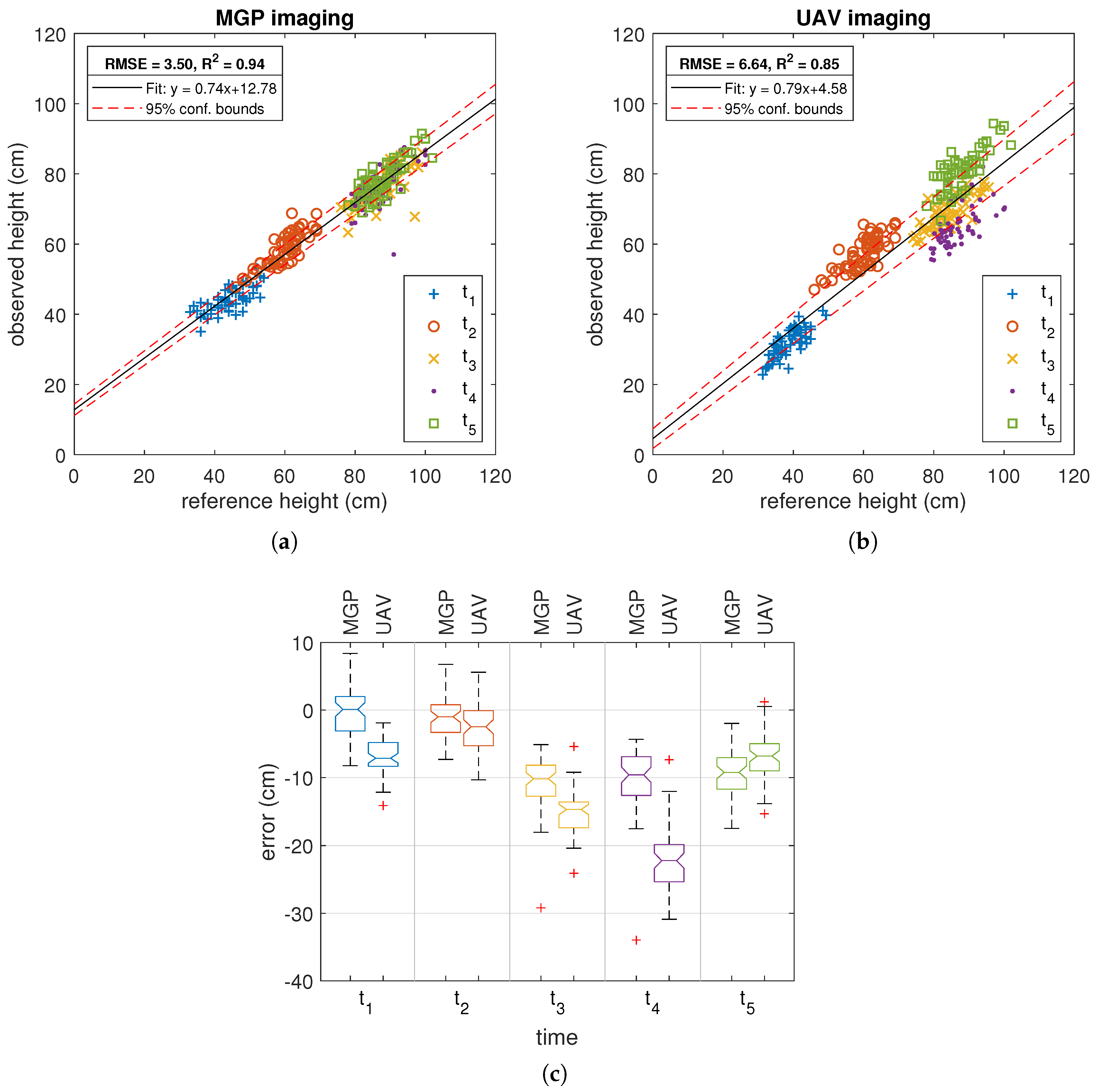
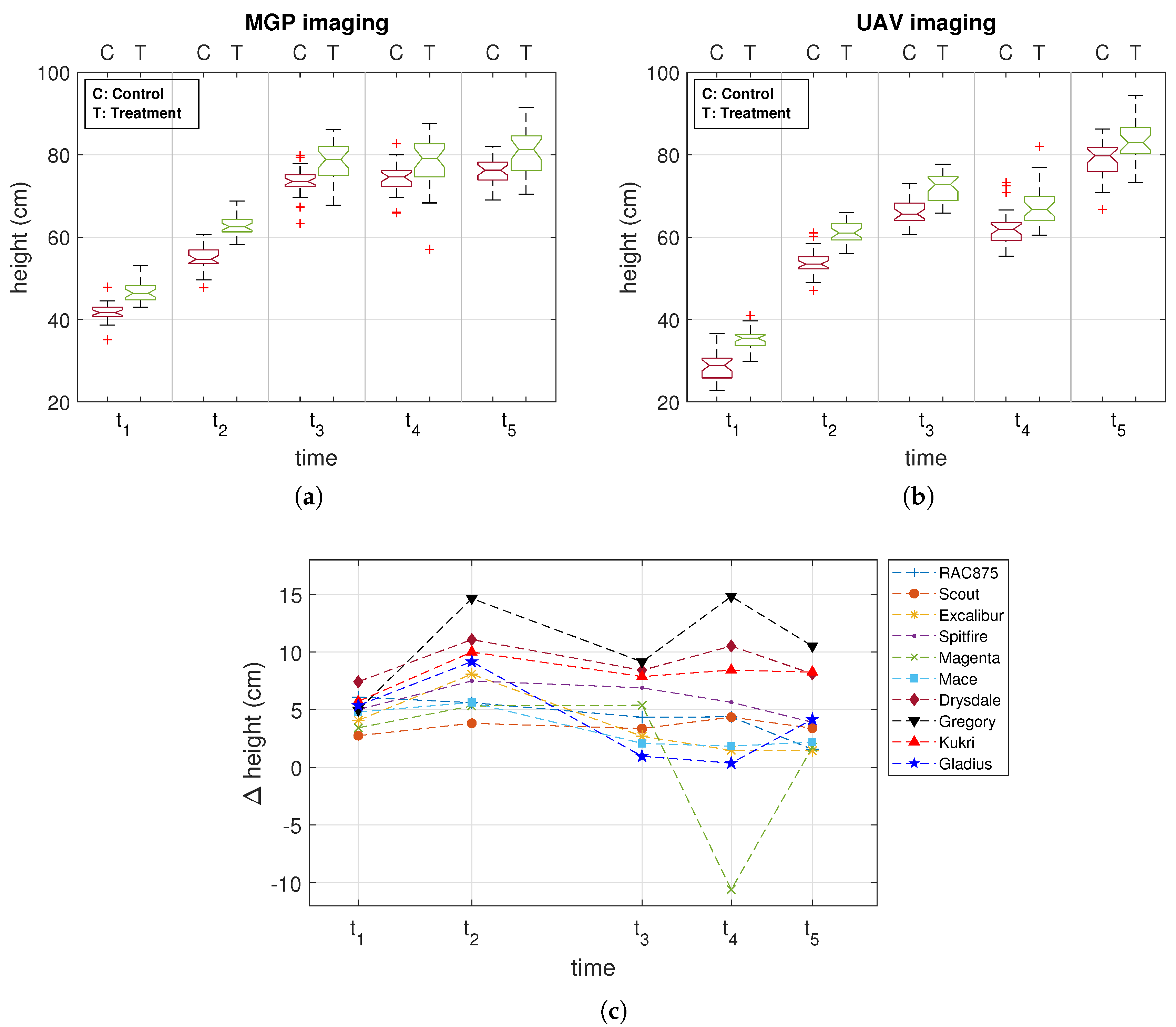
All statistical analyses were performed using the Statistics and Machine Learning Toolbox of MATLAB R2017b (Mathworks Inc., Natick, MA, USA). Canopy traits estimated from the UAV and MGP imagery were compared to the reference manual measurements using the ordinary least squares regression model with a linear and constant term. The p-value of the estimated model coefficients was derived from the t-statistics and tested against a significance level of 0.05. The goodness of fit was assessed in terms of the coefficient of determination (R${}^2$) and root mean squared error (RMSE). A significant fixed bias was found if the 95% confidence bounds of the estimated coefficient (intercept) did not contain 0. A significant proportional bias was found if the 95% confidence bounds of the estimated coefficient (the slope) did not contain 1. All errors were assumed to follow a normal distribution.

Descriptive statistics of the estimated canopy traits were summarized using box and whisker plots. The central line of a box corresponds to the median, and the lower and upper edges correspond to the first and third quartile, respectively. The whiskers extend to the extreme inlier points, and the outliers are plotted as ‘+’. The medians are significantly different at $\alpha$ = 0.05, if their notches do not overlap.

3. Results

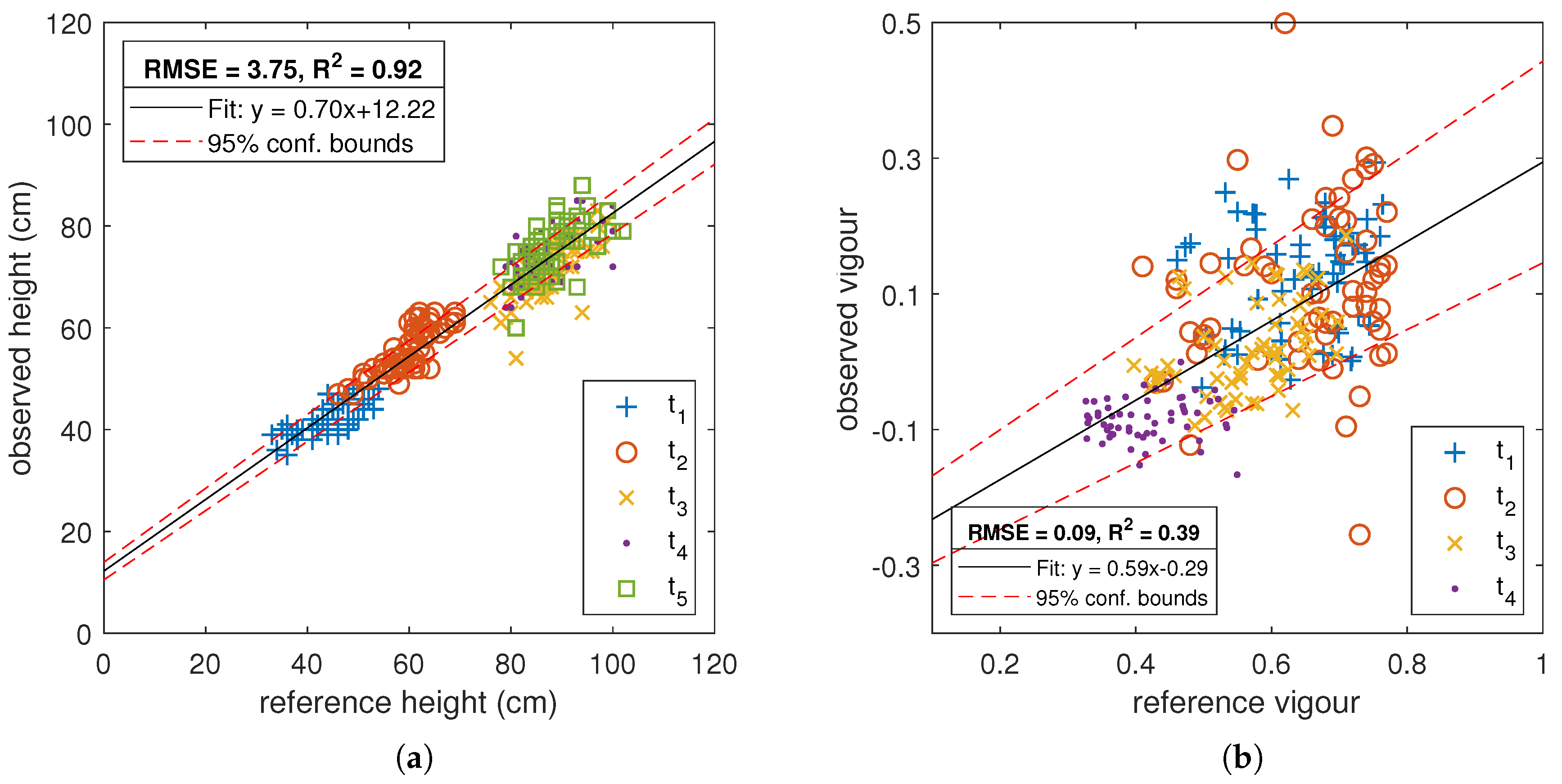
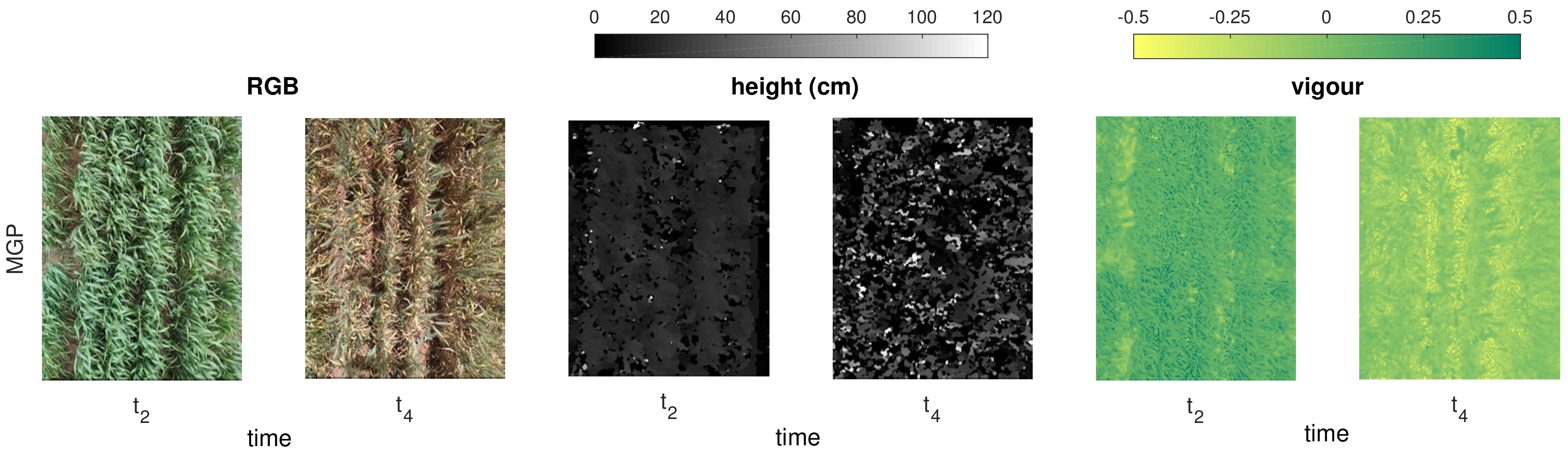
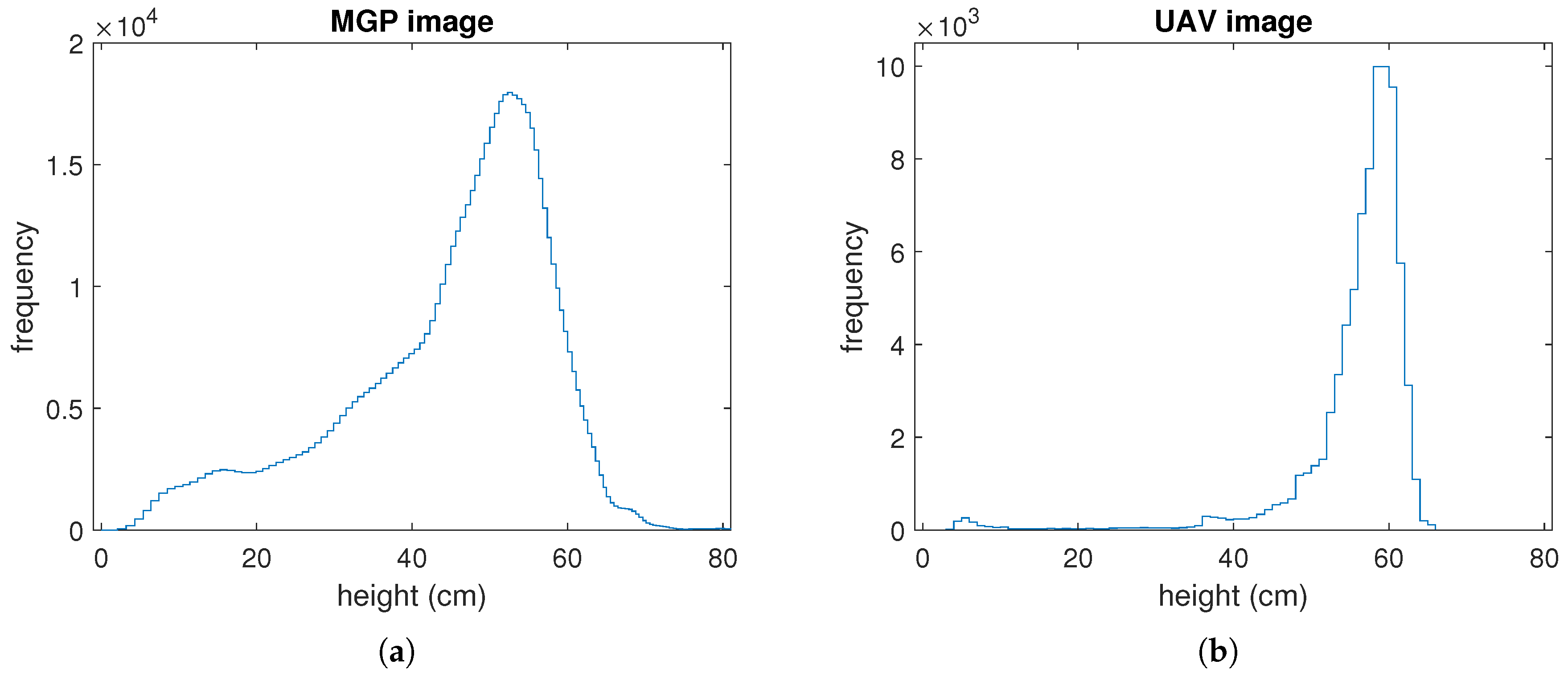
3.1. Comparison of MGP and UAV Estimated Canopy Height

The canopy height estimates of all plots derived from UAV and MGP images are compared against reference ruler measurements in Figure 2a,b. Canopy height estimates from MGP imagery had a better overall fit (RMSE = 3.95 cm, R${}^2$ = 0.94) with manual measurements, compared with estimates derived from UAV imagery (RMSE = 6.64 cm, R${}^2$ = 0.85). The 95% confidence bounds of the regression coefficients confirmed a 12.8-cm fixed bias in heights estimated by MGP imaging and a 4.6-cm fixed bias in heights estimated by UAV imaging. Both MGP and UAV imaging methodologies contained a significant proportional bias, which resulted in an underestimation of canopy height.

Height estimates relevant to different time points (growth stages) were also analysed in order to assess if there was a significant variation in estimation accuracy over time. Figure 2c shows that MGP imaging resulted in median errors closer to zero in the early growth stages $t_1$ and $t_2$. UAV imaging, however, consistently underestimated canopy heights at all time points.

With regard to the effect of fertilizer treatment, we demonstrate in Figure 3a,b that the median of canopy heights of plots in the group of treated plots was significantly higher than the heights of plots in the control group, across all five time points. This effect has been captured by both the MGP and UAV imaging system. Thus, although UAV imaging generally gave rise to greater errors (relative to the reference manual measurements), the relative difference in canopy heights between treated and untreated plots was reliably captured.

The results shown in Figure 3a,b distinguish treated plots from control plots, but otherwise collate results for the different varieties. A more detailed picture, as captured by the MGP imaging system, is shown in Figure 3c, which depicts the progressive growth difference due to fertilizer treatment for individual varieties. For each variety, the graph was drawn from the average canopy height over three replicates of treated plots minus the average canopy height over three replicates of control plots. As expected, there was a positive margin in the heights of fertilized and unfertilized plots, for most varieties. Note that a steep descent in growth difference of the Magenta variety from $t_3$–$t_4$ could be traced back to an erroneous estimate of height by MGP imagery.

We note the characteristic shape of most growth difference curves, which plateau around $t_3$, the post-anthesis stage of development. Thereafter, there is a minimal difference in plant height for most varieties except for Gregory, Drysdale and Kukri, which maintain a differential height until maturity. The differences between like-treated varieties are subtle and may require a more detailed examination than can be discussed here. Of particular relevance to these observations is the fact that the MGP-based methodology is able to quantitatively capture the temporal change, as well as the differences between the heights of the treated and untreated plots of the same variety.

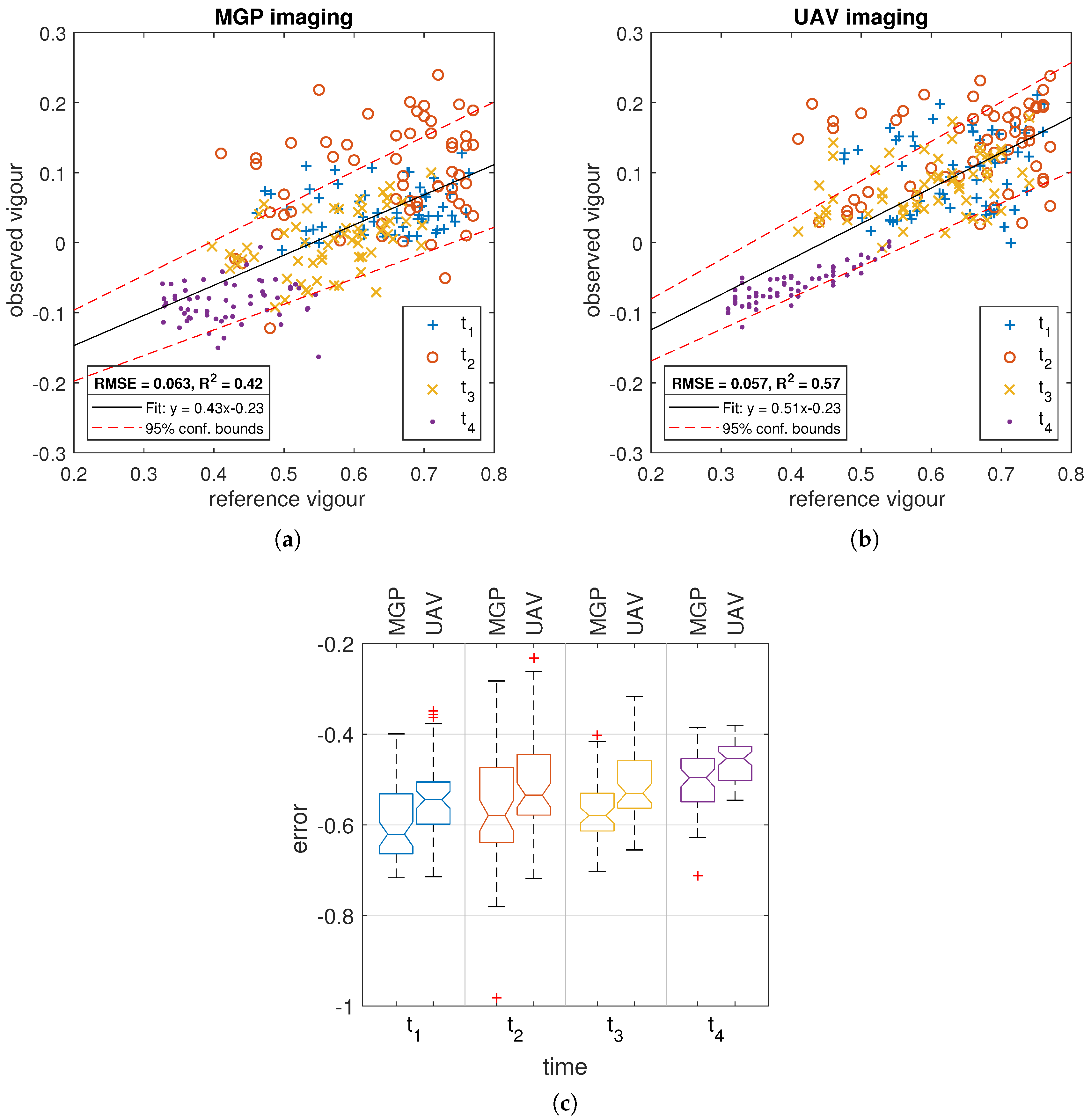
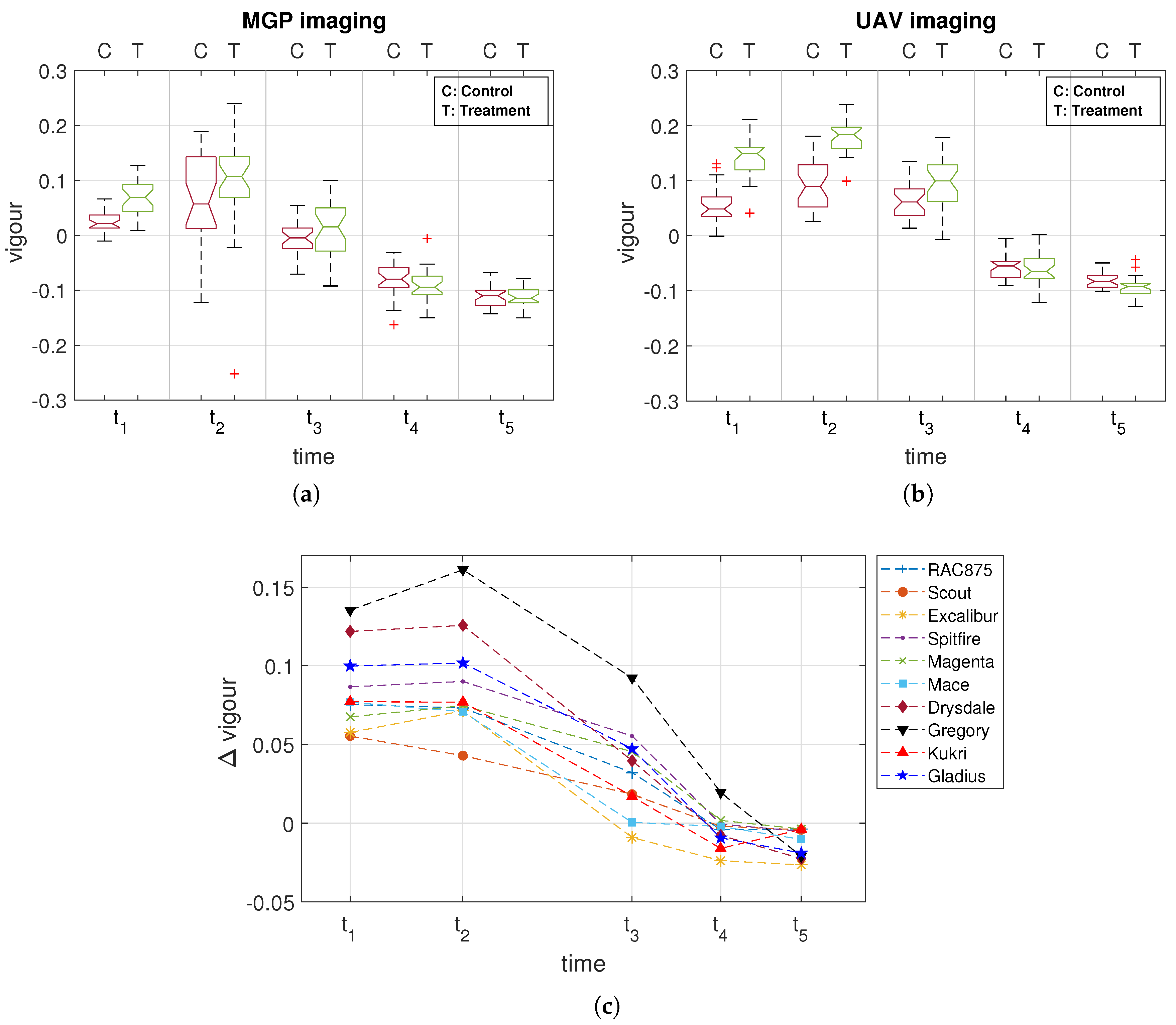
3.2. Comparison of MGP and UAV Estimated Canopy Vigour

Canopy vigour of all plots derived from MGP and UAV imagery is compared to reference hand-held sensor measurements in Figure 4a,b. In contrast to the situation with height estimates, the linear regression models associated with canopy vigour estimates by UAV imaging had slightly better agreement with reference measurements (RMSE = 0.057, R${}^2$ = 0.57) than did estimates based on MGP imaging (RMSE = 0.063, R${}^2$ = 0.42). The 95% confidence limits of regression coefficients suggested a statistically-significant fixed and proportional bias in both MGP- and UAV-derived vigour estimates.

Vigour estimation analysed at different time points (Figure 4c) revealed a significant difference between the median error of estimates provided by MGP imaging and UAV imaging, except at $t_2$. The median errors appear to be relatively lower using UAV imaging, which is consistent with the above finding, and particularly so at the later time points ($t_3$ and $t_4$).

An analysis of the effect of fertilizer application (Figure 5a,b) suggested significantly higher median canopy vigour in the treated plots at the first two time points ($t_1$ and $t_2$). The margin of median vigour between treated and control plots was higher as captured by UAV imaging in comparison to MGP imaging. Moreover, the variance within each group was lower in the case of UAV imaging compared with MGP imaging. The difference between median vigour values of the treated and control plots diminished with time and all but disappeared by the mature time points ($t_4$ and $t_5$), at which point a significant degree of senescence appears and becomes a dominant feature of the canopies.

To complement the analysis summarized in Figure 5a,b, we show the differential development of vigour in different treatments of individual varieties as captured by the UAV imaging system in Figure 5c. For each variety, the graph was drawn from the average canopy vigour over three replicates of treated plots minus the average canopy vigour over three replicates of control plots. We note the characteristic shape of the differential vigour growth curves, which decayed after $t_2$, the elongation stage of development. As in the case of canopy height, canopy vigour of varieties demonstrated different degrees of margin between treatments, with the differences becoming negligible (or negative) as the canopies degrade with increased senescence ($t_4$ and $t_5$). The greatest difference in canopy vigour between fertilized and unfertilized plots was observed at time point ($t_2$), which approximately concluded the major rainfall period of the season. Provided the canopy vigour estimates were not reliable after $t_3$, a $\Delta$vigour < 0 may have been attributed to a delayed senescence of untreated plots of some varieties than treated plots. For example, Kukri had $\Delta$vigour < 0 at $t_4$, but close to zero at $t_5$. It is possible that other varieties also reached $\Delta$vigour = 0 at a later point when both treated and control plots were fully senesced. Overall, UAV imaging was able to quantitatively capture the temporal changes in vigour significantly up to $t_3$ at the least, as well as the differences between the vigour of the treated and untreated plots of the same variety.

It is important to visually highlight the key differences in the quality of MGP and UAV images, and their derived height and vigour maps, respectively, for trait estimation. Figure 6 shows sample RGB, height and vigour images of a plot as derived from MGP and UAV imaging at two contrasting times of growth, $t_2$ and $t_4$. Note the clarity of plant leaves in the MGP image, and its corresponding height and vigour are accurately captured over time. Conversely, the RGB image captured by UAV at $t_4$ is of relatively poor quality compared to the same at $t_2$, which also translated into poor quality trait images. In general, the UAV-derived trait images barely contain as detailed information as the MGP-derived trait images. However, they are still able to provide reasonable overall estimate of traits from the noisy, but complete information of a plot. Similar results were obtained with reduced resolution MGP images, details of which can be found in Appendix A.

4. Discussion

Holman et al. [16] presented a study that addressed questions similar to those posed here, despite in comparison to a different land-based platform. In combination, the two studies are useful in establishing comparative benchmarks for field phenotyping with UAV and MGP technologies and methodologies. The scope covered by the two works not only includes a diverse set of wheat varieties (25 in [16] and 10 in this study), but also a greater range of climates, weather and (sun) lighting conditions. Consequently, the findings of these studies, in terms of the correlation between UAV imaging estimates of height and vigour, add support to the common conclusion of the two. From a broader perspective, our findings are consistent with those of [16] in terms of a favourable comparison of heights derived from UAV images with rule measurements, as well as the correlation with treatment.

A distinct advantage of the MGP imaging system is its ability to provide high resolution images of plots. Indeed, the high resolution not only allows for a greater degree of accuracy for the overall analysis of plots, it also offers the possibility of characterizing structure within the canopy. Plant leaves as a function of height can be distinguished from the terrain allowing for a detailed description of leaf density distribution and related leaf vigour distribution, as well as an accurate estimation of canopy height and overall canopy vigour that have been featured here. On the former note, leaf height and vigour distributions can be used to the advantage of more accurate estimation of canopy coverage. Moreover, a colour analysis with leaf depth distribution can facilitate assessment of the onset and progression of senescence through a canopy. Furthermore, the accuracy of plant segmentation can be improved by utilizing the combination of pixel height and colour information as a determinant to distinguish desired plant objects from surrounding mosses and weeds. The major disadvantage of MGP phenotyping is the limited spatial domain that can be covered within a reasonable period of time and with a reasonable demand on labour. In contrast, the main advantage of UAV-based phenotyping is its high-throughput capability. Excluding setup time, on average, it took 3 min for UAV imaging of the trial (~20 plots per min) compared to 30 min for MGP imaging (~2 plots per min). A major limitation though is its lower spatial resolution, which may need consideration by the end-user depending on any further information sought from the images. Here, we focused on canopy height and canopy vigour, which can be captured by the UAV system with a reasonable accuracy.

The technical differences between the image processing methodologies also affect the accuracy of trait estimates. Multi-view stereo was used to reconstruct the three-dimensional structure from synchronously-captured field images taken with the MGP. In contrast, the SfM technique was used to reconstruct three-dimensional information from time-lapse UAV images. The SfM technique assumes a stationary scene relative to the camera position. In practice, however, a completely stationary scene is rarely possible to achieve in the field as plants are susceptible to deformation (bending and twisting) through the action of wind. Since height estimates were obtained from depth maps, a few examples revealed that anomalies could be traced back to poor surface reconstruction of the plot canopy. The percentile rank of elevation in affected plots was much different than the reference elevation. Hence, the accuracy of height estimates based on UAV images was inferior to that of the MGP system, which demonstrated a greater reliability in noisy conditions (see also the discussion on structure from motion in [16]). Another differentiating feature is that aerial images are orthorectified, i.e., geometrically corrected to present a uniform scale, and mosaicked, i.e., multiple aerial images are joined together to form one large image. Canopy vigour, however, was relatively less affected by the surface reconstruction errors since it was dependent on average VI reflectance per plot.

It would be fair to say that the results of this study have substantiated canopy height and canopy vigour as relevant quantitative traits to capture and assess plot growth and health and their respective dependencies on treatment, as well as genotype. For instance, the median canopy heights of all treated plots increased at a higher rate than did those of the control plots up until maturity. Similarly, the treated canopies exhibited greater vigour compared to the control plots, although predominantly in the early stages of growth; the significant differences in vigour diminished with the onset of senescence as plants grew into maturity. At the level of individual varieties, the MGP imaging system accurately captured the different growth rates of the ten varieties, both treated and untreated, using canopy height as a quantitative measure, while the UAV imaging system best captured the differing degrees to which the varieties exhibited vigour. The slightly better agreement of manually-measured canopy heights with the MGP-based estimates can be attributed to two issues: the higher resolution of MGP imagery and its superior 3D reconstruction methodology and, conversely, the lower resolution of UAV imagery and its inferior 3D reconstruction by SfM due to the non-stationarity of plants.

Given the brevity of time between manual height measurements and UAV imaging of the field, it is unlikely that significant errors in the comparison were introduced by the interpolation of measurements. On the other hand, the interpolation of manually-conducted GreenSeeker measurements is more likely to be a contributing factor to the less accurate agreement of MGP-based estimates of vigour compared with UAV-based estimates. It is arguably the case that a plant’s GreenSeeker values can exhibit a greater variation over a shorter period of time in response to a locally changing environment. Finally, it should be remembered that while correlated, our definition of vigour is fundamentally different from the definition of the NDVI detected by the GreenSeeker sensor. This difference may also be a contributing factor to its lower correlation with image-based vigour measurement by both MGP and UAV imaging systems [29].

Continuous monitoring of crop growth using imaging systems with geospatial information is key to many applications in precision agriculture [46,47]. Of particular significance is the monitoring of canopy height and canopy vigour, which are two good indicators of crop growth. The results presented here not only confirm that these traits can be used to analyse crop responses to changes in treatment, but also prove that these indicators can be reliably obtained either by MGP or UAV imaging. Analysis of the crop growth as a function of interactions with soil and environmental conditions can subsequently provide customized management plans for farmers to maximize yield [48].

5. Conclusions

In this study, we employed UAV and MGP imaging to quantify two canopy traits, height and vigour, for a wheat field trial featuring ten wheat varieties and two treatments. The estimates derived from UAV images and MGP images were validated through a comparison with corresponding manual reference measurements of the traits taken over the course of the season. MGP imaging was found to provide better estimates of height using high resolution images of plot canopy. UAV imaging was found to provide better estimates of canopy vigour. Canopies treated with fertilizer were observed to grow taller, throughout the season, compared to untreated canopies. Treated canopies were observed to exhibit greater vigour than untreated canopies in the early stages of growth, whereas no significant difference could be detected at later stages. Both UAV and MGP imaging and analysis methods were sufficiently accurate to quantify these features.

Field phenotyping is challenging from a number of perspectives. Determining the most appropriate system depends on the application. UAV imaging is a fast and efficient means of covering a large area of land in a short time and is sufficiently accurate for canopy-wide trait estimation. MGP imaging is potentially low-throughput (depending on the platform used) and more labour intensive. However, it can capture detailed canopy structure with high fidelity, which offers the potential for trait analysis at the plant level.

References

1. Salisbury, F.B.; Ross, C.W. Plant Physiology, 4th ed.; Wadsworth Publishing: Belmont, CA, USA, 1992. [Google Scholar]
2. Patrick, A.; Li, C. High throughput phenotyping of blueberry bush morphological traits using unmanned aerial systems. Remote Sens. 2017, 9, 1250. [Google Scholar] [CrossRef]
3. Gnädinger, F.; Schmidhalter, U. Digital counts of maize plants by unmanned aerial vehicles (UAVs). Remote Sens. 2017, 9. [Google Scholar] [CrossRef]
4. Virlet, N.; Sabermanesh, K.; Sadeghi-Tehran, P.; Hawkesford, M.J. Field Scanalyzer: An automated robotic field phenotyping platform for detailed crop monitoring. Funct. Plant Biol. 2017, 44, 143–153. [Google Scholar] [CrossRef]
5. Cai, J.; Kumar, P.; Chopin, J.; Miklavcic, S.J. Land-based crop phenotyping by image analysis: Accurate estimation of canopy height distributions using stereo images. PLoS ONE 2018, 13, e0196671. [Google Scholar] [CrossRef] [PubMed]
6. Deery, D.; Jimenez-Berni, J.; Jones, H.; Sirault, X.; Furbank, R. Proximal remote sensing buggies and potential applications for field-based phenotyping. Agronomy 2014, 4, 349–379. [Google Scholar] [CrossRef]
7. Schirrmann, M.; Giebel, A.; Gleiniger, F.; Pflanz, M.; Lentschke, J.; Dammer, K.H. Monitoring agronomic parameters of winter wheat crops with low-cost UAV imagery. Remote Sens. 2016, 8, 706. [Google Scholar] [CrossRef]
8. de Castro, A.I.; Torres-Sánchez, J.; Peña, J.M.; Jiménez-Brenes, F.M.; Csillik, O.; López-Granados, F. An automatic Random Forest-OBIA algorithm for early weed mapping between and within crop rows using UAV imagery. Remote Sens. 2018, 10, 285. [Google Scholar] [CrossRef]
9. Haghighattalab, A.; Pérez, L.G.; Mondal, S.; Singh, D.; Schinstock, D.; Rutkoski, J.; Ortiz-Monasterio, I.; Singh, R.P.; Goodin, D.; Poland, J. Application of unmanned aerial systems for high throughput phenotyping of large wheat breeding nurseries. Plant Methods 2016, 12, 35. [Google Scholar] [CrossRef] [PubMed]
10. Kipp, S.; Mistele, B.; Baresel, P.; Schmidhalter, U. High-throughput phenotyping early plant vigour of winter wheat. Eur. J. Agron. 2014, 52, 271–278. [Google Scholar] [CrossRef]
11. Di Gennaro, S.F.; Rizza, F.; Badeck, F.W.; Berton, A.; Delbono, S.; Gioli, B.; Toscano, P.; Zaldei, A.; Matese, A. UAV-based high-throughput phenotyping to discriminate barley vigour with visible and near-infrared vegetation indices. Int. J. Remote Sens. 2017. [Google Scholar] [CrossRef]
12. Watanabe, K.; Guo, W.; Arai, K.; Takanashi, H.; Kajiya-Kanegae, H.; Kobayashi, M.; Yano, K.; Tokunaga, T.; Fujiwara, T.; Tsutsumi, N.; et al. High-throughput phenotyping of sorghum plant height using an unmanned aerial vehicle and its application to genomic prediction modeling. Front. Plant. Sci. 2017, 8, 421. [Google Scholar] [CrossRef] [PubMed]
13. Chen, D.; Shi, R.; Pape, J.M.; Neumann, K.; Arend, D.; Graner, A.; Chen, M.; Klukas, C. Predicting plant biomass accumulation from image-derived parameters. GigaScience 2018, 7, giy001. [Google Scholar] [CrossRef] [PubMed]
14. Kirk, K.; Andersen, H.J.; Thomsen, A.G.; Jørgensen, J.R.; Jørgensen, R.N. Estimation of leaf area index in cereal crops using red–green images. Biosyst. Eng. 2009, 104, 308–317. [Google Scholar] [CrossRef]
15. Makanza, R.; Zaman-Allah, M.; Cairns, J.E.; Magorokosho, C.; Tarekegne, A.; Olsen, M.; Prasanna, B.M. High-Throughput Phenotyping of Canopy Cover and Senescence in Maize Field Trials Using Aerial Digital Canopy Imaging. Remote Sens. 2018, 10, 330. [Google Scholar] [CrossRef]
16. Holman, F.H.; Riche, A.B.; Michalski, A.; Castle, M.; Wooster, M.J.; Hawkesford, M.J. High throughput field phenotyping of wheat plant height and growth rate in field plot trials using UAV based remote sensing. Remote Sens. 2016, 8, 1031. [Google Scholar] [CrossRef]
17. Jimenez-Berni, J.A.; Deery, D.M.; Rozas-Larraondo, P.; Condon, A.T.G.; Rebetzke, G.J.; James, R.A.; Bovill, W.D.; Furbank, R.T.; Sirault, X.R. High throughput determination of plant height, ground cover, and above-ground biomass in wheat with LiDAR. Front. Plant. Sci. 2018, 9, 237. [Google Scholar] [CrossRef] [PubMed]
18. Benedetti, R.; Rossini, P. On the use of NDVI profiles as a tool for agricultural statistics: The case study of wheat yield estimate and forecast in Emilia Romagna. Remote Sens. Environ. 1993, 45, 311–326. [Google Scholar] [CrossRef]
19. Panda, S.S.; Ames, D.P.; Panigrahi, S. Application of vegetation indices for agricultural crop yield prediction using neural network techniques. Remote Sens. 2010, 2, 673–696. [Google Scholar] [CrossRef]
20. Moriondo, M.; Maselli, F.; Bindi, M. A simple model of regional wheat yield based on NDVI data. Eur. J. Agron. 2007, 26, 266–274. [Google Scholar] [CrossRef]
21. Raun, W.R.; Solie, J.B.; Johnson, G.V.; Stone, M.L.; Lukina, E.V.; Thomason, W.E.; Schepers, J.S. In-season prediction of potential grain yield in winter wheat using canopy reflectance. Agron. J. 2001, 93, 131–138. [Google Scholar] [CrossRef]
22. Magney, T.S.; Eitel, J.U.H.; Huggins, D.R.; Vierling, L.A. Proximal NDVI derived phenology improves in-season predictions of wheat quantity and quality. Agric. For. Meteorol. 2016, 217, 46–60. [Google Scholar] [CrossRef]
23. Hamuda, E.; Glavin, M.; Jones, E. A survey of image processing techniques for plant extraction and segmentation in the field. Comput. Electron. Agric. 2016, 125, 184–199. [Google Scholar] [CrossRef]
24. Meyer, G.E.; Neto, J.C. Verification of color vegetation indices for automated crop imaging applications. Comput. Electron. Agric. 2008, 63, 282–293. [Google Scholar] [CrossRef]
25. Mao, W.; Wang, Y.; Wang, Y. Real-time detection of between-row weeds using machine vision. In Proceedings of the ASAE Annual Meeting. American Society of Agricultural and Biological Engineers, Las Vegas, NV, USA, 27–30 July 2003. [Google Scholar]
26. Motohka, T.; Nasahara, K.N.; Oguma, H.; Tsuchida, S. Applicability of green-red vegetation index for remote sensing of vegetation phenology. Remote Sens. 2010, 2, 2369–2387. [Google Scholar] [CrossRef]
27. Rasmussen, J.; Ntakos, G.; Nielsen, J.; Svensgaard, J.; Poulsen, R.N.; Christensen, S. Are vegetation indices derived from consumer-grade cameras mounted on UAVs sufficiently reliable for assessing experimental plots? Eur. J. Agron. 2016, 74, 75–92. [Google Scholar] [CrossRef]
28. Hunt, E.R.; Cavigelli, M.; Daughtry, C.S.; Mcmurtrey, J.E.; Walthall, C.L. Evaluation of digital photography from model aircraft for remote sensing of crop biomass and nitrogen status. Precis. Agric. 2005, 6, 359–378. [Google Scholar] [CrossRef]
29. Hoffmann, H.; Jensen, R.; Thomsen, A.; Nieto, H.; Rasmussen, J.; Friborg, T. Crop water stress maps for an entire growing season from visible and thermal UAV imagery. Biogeosciences 2016, 13, 6545. [Google Scholar] [CrossRef]
30. Montes, J.M.; Technow, F.; Dhillon, B.S.; Mauch, F.; Melchinger, A.E. High-throughput non-destructive biomass determination during early plant development in maize under field conditions. Field Crops Res. 2011, 121, 268–273. [Google Scholar] [CrossRef]
31. Mistele, B.; Schmidhalter, U. Spectral measurements of the total aerial N and biomass dry weight in maize using a quadrilateral-view optic. Field Crops Res. 2008, 106, 94–103. [Google Scholar] [CrossRef]
32. Mistele, B.; Schmidhalter, U. Tractor-based quadrilateral spectral reflectance measurements to detect biomass and total aerial nitrogen in winter wheat. Agron. J. 2010, 102, 499–506. [Google Scholar] [CrossRef]
33. Andrade-Sanchez, P.; Gore, M.A.; Heun, J.T.; Thorp, K.R.; Carmo-Silva, A.E.; French, A.N.; Salvucci, M.E.; White, J.W. Development and evaluation of a field-based high-throughput phenotyping platform. Funct. Plant Biol. 2014, 41, 68–79. [Google Scholar] [CrossRef] [Green Version]
34. Freeman, K.W.; Girma, K.; Arnall, D.B.; Mullen, R.W.; Martin, K.L.; Teal, R.K.; Raun, W.R. By-plant prediction of corn forage biomass and nitrogen uptake at various growth stages using remote sensing and plant height. Agron. J. 2007, 99, 530–536. [Google Scholar] [CrossRef]
35. White, J.W.; Conley, M.M. A flexible, low-cost cart for proximal sensing. Crop Sci. 2013, 53, 1646–1649. [Google Scholar] [CrossRef]
36. Candiago, S.; Remondino, F.; De Giglio, M.; Dubbini, M.; Gattelli, M. Evaluating multispectral images and vegetation indices for precision farming applications from UAV images. Remote Sens. 2015, 7, 4026–4047. [Google Scholar] [CrossRef]
37. Gracia-Romero, A.; Kefauver, S.C.; Vergara-Diaz, O.; Zaman-Allah, M.A.; Prasanna, B.M.; Cairns, J.E.; Araus, J.L. Comparative performance of ground versus aerially assessed RGB and multispectral indices for early-growth evaluation of maize performance under phosphorus fertilization. Front. Plant. Sci. 2017, 8, 2004. [Google Scholar] [CrossRef] [PubMed]
38. Vergara-Díaz, O.; Zaman-Allah, M.A.; Masuka, B.; Hornero, A.; Zarco-Tejada, P.; Prasanna, B.M.; Cairns, J.E.; Araus, J.L. A Novel Remote Sensing Approach for Prediction of Maize Yield Under Different Conditions of Nitrogen Fertilization. Front. Plant Sci. 2016, 7. [Google Scholar] [CrossRef] [PubMed]
39. Liebisch, F.; Kirchgessner, N.; Schneider, D.; Walter, A.; Hund, A. Remote, aerial phenotyping of maize traits with a mobile multi-sensor approach. Plant Methods 2015, 11, 9. [Google Scholar] [CrossRef] [PubMed]
40. Madec, S.; Baret, F.; De Solan, B.; Thomas, S.; Dutartre, D.; Jezequel, S.; Hemmerlé, M.; Colombeau, G.; Comar, A. High-throughput phenotyping of plant height: Comparing unmanned aerial vehicles and ground LiDAR estimates. Front. Plant Sci. 2017, 8, 2002. [Google Scholar] [CrossRef] [PubMed]
41. Chopin, J.; Kumar, P.; Miklavcic, S.J. Land-based crop phenotyping by image analysis: Consistent canopy characterization from inconsistent field illumination. Plant Methods 2018, 14, 39. [Google Scholar] [CrossRef] [PubMed]
42. Hirschmueller, H. Stereo processing by semiglobal matching and mutual information. Trans. Pattern Anal. Mach. Intell. 2008, 30, 328–341. [Google Scholar] [CrossRef] [PubMed]
43. Koenderink, J.J.; Van Doorn, A.J. Affine structure from motion. J. Opt. Soc. Am. A 1991, 8, 377–385. [Google Scholar] [CrossRef] [PubMed]
44. Heikkila, J.; Silven, O. A four-step camera calibration procedure with implicit image correction. In Proceedings of the Conference on Computer Vision and Pattern Recognition, San Juan, Puerto Rico, USA, 17–19 June 1997; pp. 1106–1112. [Google Scholar] [Green Version]
45. Khan, Z.; Rahimi-Eichi, V.; Haefele, S.; Garnett, T.; Miklavcic, S.J. Estimation of vegetation indices for high-throughput phenotyping of wheat using aerial imaging. Plant Methods 2018, 14, 20. [Google Scholar] [CrossRef] [PubMed] [Green Version]
46. Zhang, C.; Kovacs, J.M. The application of small unmanned aerial systems for precision agriculture: A review. Precis. Agric. 2012, 13, 693–712. [Google Scholar] [CrossRef]
47. Mulla, D.J. Twenty five years of remote sensing in precision agriculture: Key advances and remaining knowledge gaps. Biosyst. Eng. 2013, 114, 358–371. [Google Scholar] [CrossRef]
48. Ni, J.; Yao, L.; Zhang, J.; Cao, W.; Zhu, Y.; Tai, X. Development of an unmanned aerial vehicle-borne crop-growth monitoring system. Sensors 2017, 17, 502. [Google Scholar] [CrossRef] [PubMed]
Figure 1. (a) The MGP with stereo imaging cameras and calibration target. (b) The UAV with the camera payload. (c) A perspective view of the trial site with ground control points magnified as insets. The red broken line shows the aerial path taken by the UAV.
Remotesensing 10 00950 g001
Figure 2. Regression analysis of canopy height estimates for (a) MGP imaging and (b) UAV imaging, relative to reference heights. (c) Distribution of height estimation errors with time, t n .
Remotesensing 10 00950 g002
Figure 3. Canopy heights of treated and control plots at time point t n as derived from (a) MGP imaging and (b) UAV imaging. The data shown summarize the results over the 60 plots: 10 varieties and three replicates for each treatment. (c) Difference between average canopy height of treated and untreated plots of each variety derived from MGP imagery (time axis scaled to actual duration).
Remotesensing 10 00950 g003
Figure 4. Regression analysis of canopy vigour estimates for (a) MGP imaging and (b) UAV imaging, relative to reference vigour. (c) Distribution of vigour estimation errors with time, t n .
Remotesensing 10 00950 g004
Figure 5. Canopy vigour of treated and control plots at time point t n as derived from (a) MGP imaging and (b) UAV imaging. The data shown summarize the results over the 60 plots: 10 varieties and three replicates for each treatment. (c) Difference between average canopy vigour of treated and untreated plots of each variety derived from UAV imagery (time axis scaled to actual duration).
Remotesensing 10 00950 g005
Figure 6. RGB, height and vigour of a wheat plot at time t 2 and t 4 derived from MGP imaging (top) and UAV imaging (bottom). For the purpose of visualization, the illustrated MGP images are a result of stitching the three partial images per plot using Image Composite Editor (Microsoft) software.
Remotesensing 10 00950 g006