A Novel Approach for the Short-Term Forecast of the Effective Cloud Albedo


1
Faculty of Geography, Deutscher Wetterdienst, Frankfurter Straße 135, 63067 Offenbach, Germany
2
Philipps-Universität Marburg, Deutschhausstraße 12, 35032 Marburg, Germany
*
Author to whom correspondence should be addressed.
Remote Sens. 2018, 10(6), 955; https://0-doi-org.brum.beds.ac.uk/10.3390/rs10060955
Submission received: 27 April 2018
/
Revised: 23 May 2018
/
Accepted: 8 June 2018
/
Published: 15 June 2018
(This article belongs to the Section Atmospheric Remote Sensing)
Abstract
:The increasing use of renewable energies as a source of electricity has led to a fundamental transition of the power supply system. The integration of fluctuating weather-dependent energy sources into the grid already has a major impact on its load flows. As a result, the interest in forecasting wind and solar radiation with a sufficient accuracy over short time periods (<4 h) has grown. In this study, the short-term forecast of the effective cloud albedo based on optical flow estimation methods is investigated. The optical flow method utilized here is TV-L1 from the open source library OpenCV. This method uses a multi-scale approach to capture cloud motions on various spatial scales. After the clouds are displaced, the solar surface radiation will be calculated with SPECMAGIC NOW, which computes the global irradiation spectrally resolved from satellite imagery. Due to the high temporal and spatial resolution of satellite measurements, the effective cloud albedo and thus solar radiation can be forecasted from 5 min up to 4 h with a resolution of 0.05°. The validation results of this method are very promising, and the RMSE of the 30-min, 60-min, 90-min and 120-min forecast equals 10.47%, 14.28%, 16.87% and 18.83%, respectively. The paper gives a brief description of the method for the short-term forecast of the effective cloud albedo. Subsequently, evaluation results will be presented and discussed.

1. Introduction
The power supply system is under fundamental transition. The replacement of fossil fuels by renewable energy is progressing rapidly. Weather-dependent energy sources such as wind and solar radiation play a major role within the transition. The integration of wind and solar energy into the grid has a huge impact on the load flows. For this reason, the forecasts of solar radiation and wind have to be more precise with particular regard to the short-term forecast for up to 3–4 h. Thus, a forecast based on satellite observations, also referred to as nowcasting, is of priority choice for this issue. It shows better results for the first few hours of photovoltaic power forecasts (PV forecasts) in comparison to numerical weather prediction models (NWP) [1]. Further, NWP runs with data assimilation need usually 3–6 h of computation time. Thus, the results of the numerical weather prediction model are only available with a time delay of several hours, whereas satellite-based forecasts are available in near real time.
The temporal short-term variation of the solar surface irradiance in Central Europe is predominantly related to cloud occurrence. Thus, an accurate short-term forecast of relevant cloud properties is of high importance. The main challenge is to properly forecast the location and the shape of clouds for the next few hours from satellite data. For the forecast of clouds, we use the optical flow methods TV- and Farnebäck provided by the OpenCV library through calculating cloud motion vectors [2]. Optical flow is a widely-used and well-established technique for image pattern recognition in the fields of traffic, locomotion and face re-detection. An overview of different optical flow methods and their application is given by Sonka et al. [3]. So far, however, TV- and other optical flow methods are hardly used for the calculation of cloud motion vectors in meteorology. To our knowledge, one of the first applications has been the utilization of the optical flow for radar images as described by Peura and Hohti [4]. Optical flow has been recently implemented for the short-term forecast of radar reflectivity at the German Weather Service (“Deutscher Wetterdienst”), as well. The success of the estimation of the optical flow of radar images indicates that the method could be transferred to the forecast of clouds and their properties. A promising candidate for the forecast of cloud properties is the effective cloud albedo (CAL). CAL is derived from the reflectivity measured in the visible bands of satellites. The advantages of the effective cloud albedo are manifold. For instance, CAL can be directly observed from space, without the need for any additional model or information [5]. For CAL values up to 0.8, the cloud transmission for solar radiation is simply defined by [5]. Thus, the effective cloud albedo includes the required information about the cloud effect on the solar surface irradiance. Further, the reflection of the Earth’s surface is already filtered, allowing optical flow to focus on clouds. As a result, satellite observations enable the retrieval of the CAL and solar radiation at the ground, with high spatial and temporal resolution and a large areal coverage. For further information on the retrieval of the effective cloud albedo, the reader is referred to Müller et al. [5]. In our study, the effective cloud albedo of two subsequent images is used as the input for the estimation of the optical flow method. The estimated cloud motion vectors are then applied on the latter of these two images to extrapolate the observed cloud albedo into the future. Further details on this topic are given in Section 2.1.
Straightforward methods for the calculation of cloud motion vectors are based on the minimization of the root mean square error (RMSE) or the absolute difference between a shifted image in the x-y direction and the subsequent image. The cloud motion is defined by its shift in the x-y direction, which minimizes the RMSE or absolute difference between the images. This can be applied to various spatial scales and thus is called the multi-scale approach. Multiple scales lead to a dense vector field; however, more scales also increase the computation time needed. The cloud motion vectors applied for the satellite weather at the German Weather Service [6] are an example of a straightforward multi-scale approach, which is based on the above-described minimization of the absolute differences. Another example is the method of Schmetz et al. [7]. Here, a cross-correlation method is used for the cloud motion vectors. In this method, image filtering, also known as slicing, is applied to enhance the highest cloud tracer suitable for tracking. This filtering leads to a relative low density of cloud motion vectors, which is a significant disadvantage for energy meteorology applications. The Nowcasting Satellite Application Facility (NWCSAF) uses a similar approach, namely a gradient method, to define the cloud edges and cross-correlation for the calculation of the motion vectors [8]. This method also leads to a low density of cloud motion vectors and is therefore not appropriate for energy meteorology. Originally, the main application of satellite-derived cloud motion vectors was the use of wind fields in the data analysis for numerical weather prediction where a dense field might be less important [7]. However, only a dense field of cloud motion vectors enables a forecast with large geographical coverage and high temporal resolution without data gaps.
In the last few years, cloud motion vectors have gained significantly in importance within the scope of PV forecasts, and recently, their relevance has also been recognized for short-term forecasts of wind energy. However, a dense vector field of cloud motion vectors is a precondition for energy meteorology applications. Neural networks (NN) are therefore widely used to gain a dense vector field from high resolution satellite images with the advantage of a low computation time. Voyant et al. [9] provide a review of neural network methods applied to the forecast of solar surface radiation. A disadvantage of neural networks is their black box character. A neural network is, strictly speaking, only valid for the training framework, as only the behavior of the training datasets can be reproduced. An application to other regions, periods or satellite instruments typically requires extensive re-training. Further, the black box character hampers a deeper understanding of the involved physics and physical reasons of the uncertainties occurring.
Thus, optical flow methods might be a good alternative for the estimation of cloud motion vectors. However, they are not mentioned neither in the review of photovoltaic power forecasting performed by Antonanzas et al. [10], nor by the review of very short PV forecasting with cloud modeling by Barbieri et al. [11]. Other leading experts, for example Raza et al. [12], Perez et al. [13] or Wolff et al. [1], do not mention optical flow methods provided by OpenCV as an option for cloud forecasting. However, the optical flow of satellite images has been used for the Geometric Accuracy Investigations of the Spinning Enhanced Visible and Infrared Imager (SEVIRI) High Resolution Visible (HRV) Level 1.5 Imagery [14]. Further, Simonenko et al. [15] discussed the optical flow method TV- concerning the interpolation between observed cloud images, in order to improve the temporal information about convective volcanic ash plumes. However, neither the short-term forecast of solar surface irradiance, nor its application were addressed. As a consequence, only a few works about the application of optical flow methods for the forecast of cloud motion vectors from satellite imagery and practically no works on satellite based short-term forecast of solar surface irradiance exist. Yet, the authors are aware of only one publication in which a multiple-scale optical flow method is applied within the scope of satellite-based solar irradiance forecasts [16]. The respective method is developed within the storm detection and nowcasting system Cb-TRAM (Tracking and monitoring severe convection from onset over rapid development to the mature phase using multi-channel Meteosat-8 SEVIRI data) [17,18]. Unfortunately, the details of the method are not well described, and the software is not available in open access, which limits the scientific benefit of the work. Further, the authors applied the cloud motion vectors to cloud optical thickness and effective radius, but not to CAL. For the correct retrieval of cloud optical depth and effective radius , accurate information of the surface albedo and the atmospheric composition is needed. Furthermore, simplifications in the radiative transfer are typically applied within the retrieval of the cloud optical depth and . These items induce uncertainties in the estimation of the solar surface irradiance, which can be avoided if the satellite-observable CAL is used.
Thus, to the knowledge of the authors, the optimization of the recent TV- method and its application to the effective cloud albedo for the forecast of solar surface irradiation is a novel approach within energy meteorology. Furthermore, this work is one of the first in which the two optical flow methods of the OpenCV library (TV-, Farnebäck) are evaluated and compared in the context of cloud albedo forecasting. The authors believe that the combination of the effective cloud albedo with TV- and SPECMAGIC NOW [19] delivers a new powerful method for the short-term forecast of solar surface irradiance.
2. Materials and Methods
2.1. Optical Flow Method
Optical flow is a pattern of apparent motion of image objects between two sequential frames caused by either the movement of the object or the camera [20]. Three-dimensional motion of objects can be projected onto a two-dimensional plane by calculating the optical flow. Its result is a vector field where each vector is a displacement vector showing the movement of pixels from the first frame to the second [21]. Once computed, the optical flow can be used for a wide range of tasks [22]. It may be applied for motion detection, object segmentation, motion compensated encoding and stereo disparity measurements. On top of that, it can be used to reconstruct the three-dimensional motion of visual sensors and surface structures [21].
The optical flow works on two major assumptions, which are (1) that the pixel intensities of an object do not change between consecutive frames and (2) that neighboring pixels have similar motion. The assumption of constant intensity between two consecutive frames is valid for all of the following methods. can be expressed as follows [23]:
where represents the trajectory of a point in the image and t is the time. Applying the chain rule results in the following functional:
which is equivalent to the following linear condition called the optical flow constraint equation [24]:
This equation alone is not sufficient for the estimation of the optical flow though, because there are twice as many variables as equations because this linear equation is dependent on x and y. This linear system is therefore undetermined. At this point, many methods for the determination of the optical flow were found to solve the problem by adding various conditions, as for instance block-based methods, discrete optimization methods and differential methods [25]. The latter offers some more options, for instance the Lucas–Kanade method or the Horn–Schunck method [24,26], which were the first to extend the problem with additional conditions. Both are based on partial derivatives of the image signal or the sought flow field and higher-order partial derivatives. The most common algorithms for meteorological purposes concerning optical flow are by Farnebäck [27] and the duality-based approach of the method TV- [23,28].
The optical flow estimation by Farnebäck [27] is the older method. It uses two frames to estimate the flow. In a first step, the neighborhood of both frames has to be approximated by quadratic polynomials. This can be efficiently done by using the polynomial expansion transform. In a second step, the displacement has to be estimated with the help of the coefficients of the polynomial expansion:
where A is a matrix, b is a vector and c is a scalar. These coefficients are calculated from a weighted least squares fit to the signal value in the neighborhood. Typically, the center point has the highest weight, while the surrounding weights decrease radially. Large displacements can cause large errors in the estimated motion because the general assumption of Farnebäck is that the local polynomials at the same coordinates in the two images are identical except for a displacement. This issue can be solved by a multi-scale approach, which means that the algorithm starts at a coarse scale to get a rough displacement estimate and continues with finer scales to obtain a more accurate estimate [27].
TV- is a variational method based on the method by Horn and Schunck [24], however using other data and smoothness terms [28]. Like the Farnebäck method, TV- uses two frames to estimate the optical flow. The TV- method is based on the minimization of a functional containing a data term using the robust -norm in the data fidelity term and a regularization term using the total variation (TV) of the flow [23]. The method is based on the minimization of the following image-based error criterion:
In this formula, and denote the two image frames and denotes the disparity map, which should be found with this method. Further, the disparity map u is the minimizer of the above-mentioned criterion (Equation (5)). The term describes the image data fidelity, and represents the regularization term. Moreover, works as a weighting factor between the data fidelity and the regularization term. If one selects and , the result will be the Horn–Schunck method. As the algorithm by Farnebäck, the TV- method uses scale-space approaches and, on top of that, coarse-to-fine warping to provide solutions for optical flow estimations with large displacements. Because the algorithm contains discontinuities, it is more robust against noise than the classical approach by Horn and Schunck [24].
In the numerical implementation of both algorithms, there are several parameters to adjust the estimation of the optical flow to the sort of data with which one is working. This can range from the number of scales for the multi-scale approach to smoothing factors and the number of iterations (see Section 3.2). However, the amount of parameters differs, as well as the type of parameters of the two algorithms. The algorithm of Farnebäck uses 8 parameters, while the TV- method by Zach et al. uses 10, when settings for the inner and outer iterations are considered separately [27,28]. For further information on the technique, the reader may refer to the website of OpenCV [2].
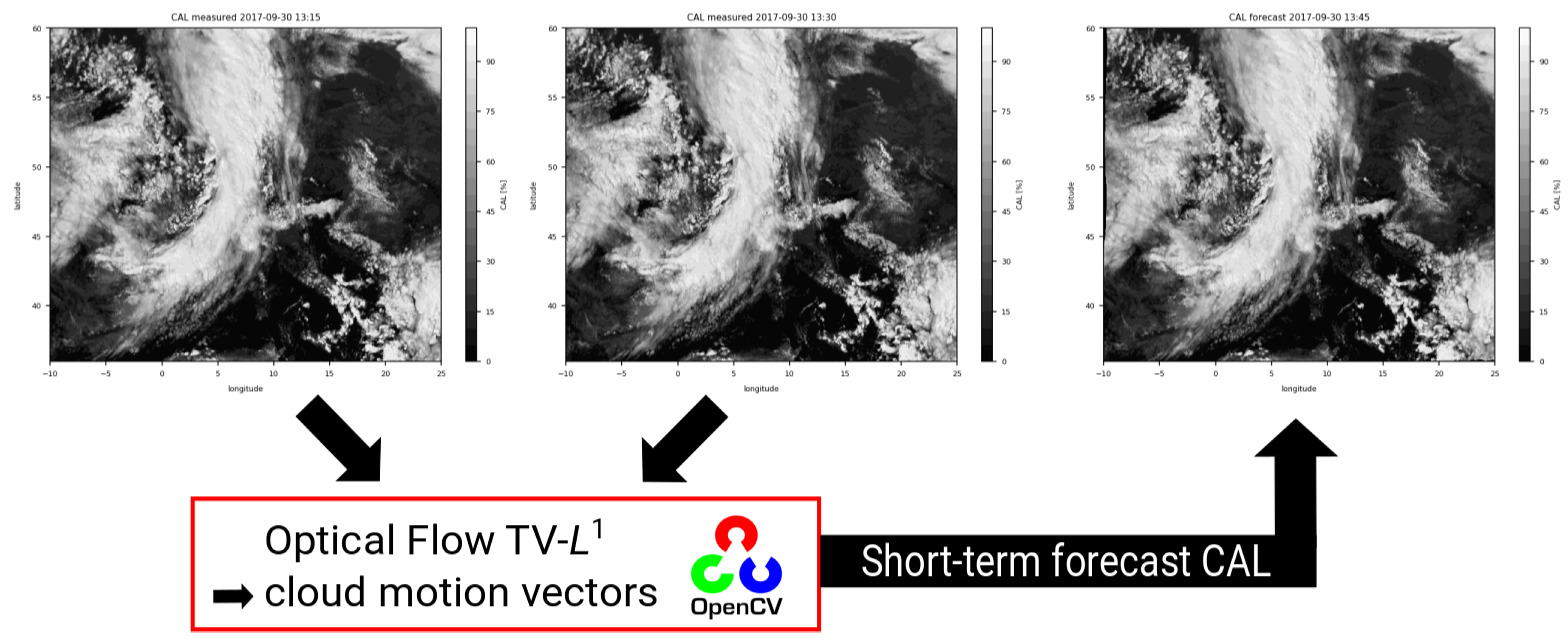
After the calculation of the motion vectors for the optical flow estimation, they need to be applied to a data field to achieve the forecast. A schematic diagram of the forecasting process is given in Figure 1. In a first step, two subsequent images of the effective cloud albedo are used as input for the TV- method (or Farnebäck method) to estimate the optical flow. TV- (Farnebäck) estimates the optical flow, which results from the differences between the two subsequent images induced by the movement of the clouds. The so-derived cloud motion vectors are then applied to the latter of the two observed CAL images in order to extrapolate the variation in CAL induced by the movement of the clouds into the future. This process can be repeated as often as desired until a certain forecast time is reached at which the NWP delivers better results than the satellite-based short-term forecast.
2.2. The Heliosat Method
The effective cloud albedo can be derived from geostationary satellites by using the observed reflectances from the visible bands without the need for any further information. The effective cloud albedo is also referred to as the cloud index by other authors [29,30,31]. Here, the visible channel at 600 nm from SEVIRI on board the Meteosat Second Generation (MSG) is used for the calculation of the effective cloud albedo. The data are provided by the European Organisation for the Exploitation of Meteorological Satellites (EUMETSAT) as rectified images of digital counts, capturing the signal of the reflection of the Earth’s atmosphere and surface.
The location of the geostationary satellites is over the Equator at 0° longitude with a field of view up to 80°N/S and 80°E/W, respectively. An example of the full disk is illustrated in Figure 2 for a clear sky reflection and effective cloud albedo case. The effective cloud albedo can be defined as the normalized difference between the all-sky and the clear-sky reflection in the visible range observed by the satellite. One minus the effective cloud albedo defines the cloud transmission for values of the albedo between 0 and 0.8. For effective cloud albedo values above 0.8, this relation will be modified in order to consider the saturation and absorption effects in optically thick clouds [5]. Due to the fact that illumination conditions may vary because of the Sun-Earth distance and the solar zenith angle, the effective cloud albedo has to be corrected. Furthermore, the dark offset of the instrument has to be subtracted from the satellite image counts. The observed reflections are therefore normalized by applying the following equation:
Here, D is the observed digital count including the dark offset of the satellite instrument. is the dark offset, which is the baseline value of the instrument in the absence of irradiance, and therefore, it has to be subtracted. The Sun-Earth distance variation is taken into account by the factor f. Finally, the cosine of the solar zenith angle corrects the different illumination conditions at the top of the atmosphere introduced by different solar elevations.
The effective cloud albedo can be derived from the normalized pixel reflection , the clear sky reflection and the maximal cloud reflection as follows:
Here, is the observed reflection for each pixel and time, and is the clear sky reflection, which is calculated according to an approach of Müller et al. [19] within the scope of spectral clear-sky reflectance. The maximum reflection is determined by the 95th percentile of all reflection values at local noon in a target region. It is characterized by a high frequency of cloud occurrence for each month. Thus, changes in the satellite brightness sensitivity are accounted for. All reflection types were corrected in the same manner using Equation (6).
Only the observed reflections are needed to derive the effective cloud albedo with the application of Equation (7). As a result, the effective cloud albedo is completely defined by the satellite observation with only one broadband visible channel needed. The accuracy and limitations of the method are discussed in Müller et al. [5].
The aim of the application of the optical flow onto the effective cloud albedo is to obtain a short-term forecast of the solar surface irradiation. First of all, the optical flow of the effective cloud albedo is used to displace the clouds, and after that, the solar surface radiation can be calculated. The solar surface irradiance is retrieved using the well-established Heliosat relation between the effective cloud albedo and the solar irradiance, which is based on the law of energy conservation [29,31]. As a consequence, the basic relation between the solar irradiance and the effective cloud albedo is predominantly a linear relation. This relation and the method to estimate the solar surface irradiation using CAL as the input is described in the work of Müller et al. [19]. For effective cloud albedo values above 0.8, the above equation is modified in order to consider the saturation and absorption effects in optically-thick clouds. The modification of the equation for small and large values of the effective cloud albedo is based on ground measurements and is described in more detail in Hammer et al. [31]. The forecast of solar surface irradiance relies on the accuracy of the forecasted effective cloud albedo. As the clear-sky variables are not forecasted, it is the only quantity of interest for the present forecast study and thus for the following results and discussion.
2.3. Verification
For the purpose of verifying the optical flow results, we calculated the absolute difference of the optical flow estimate and the measured satellite image. The unit of this result is %, as it is the unit of the effective cloud albedo, as well. This was done for all investigated cases. On top of that, three different error measures were calculated on the bases of the absolute difference. These are the bias, the absolute bias and the root mean square error. The exact calculation of the error measures is as follows (8)–(10):
3. Results
3.1. TV- Versus Farnebäck
As mentioned in Section 2.1, there were two prominent methods to estimate the optical flow for meteorological purposes. We calculated the absolute difference of the optical flow estimate and the measured satellite image as described in Section 2.3 to decide whether the Farnebäck or the TV- method performed better for the effective cloud albedo. The parameter settings for the comparison were done by eye, which is sufficient because differences can become small when setting the parameter values. The absolute difference is shown in Figure 3, and the absolute bias for this case and for another 10 exemplary cases can be found in Table 1.
First of all, the higher absolute difference of the optical flow calculated with the method by Farnebäck is obvious. Moreover, the absolute bias is 5.43% for the Farnebäck method, and it is 4.37% for the TV- method. Furthermore, the RMSE is higher for the Farnebäck method (9.53%) compared to 7.59% with TV-. Beyond this single event, the TV- method shows better results for all examined cases, so that this method is used to estimate the optical flow with the effective cloud albedo.
There are 10 different parameters in the TV- method DualTVL1OpticalFlow from OpenCV, which can be modified to influence the result of the optical flow estimation. Some parameters like the stopping criterion , the time step , as well as the inner and outer iterations can affect the speed of the algorithm. must be selected as a compromise between precision and running time. A small value gives a more accurate solution, but at the cost of a slower convergence. The time step is responsible for the stability of the algorithm. Chambolle [32] showed that the numerical scheme converges for values of . However, its value can also be set to 0.25 for a faster convergence, which was found out empirically by Sánchez et al. [23]. For the multi-scale approach mentioned in Section 1, the method needs the number of scales and the downscaling factor or so-called scale step, which is used to divide the original data to create a pyramidal structure. The value of the downscaling factor can range between zero and one. Other parameters have an influence on the shape of the forecasted clouds, for instance the data attachment weight and the tightness parameter . is the most important parameter because it determines the smoothness of the result. serves as a link between the attachment and the regularization terms. If the value of is small, the correspondence of both terms can be maintained. For our data, two of the parameters were less sensitive to the data: the illumination parameter and the number of warpings . Consequently, the setting of these parameters hardly affected the results. represents an additional illumination term, which can affect the tracking of clouds, but did not in the current analysis. Finally, describes the number of times that the specific terms were computed per scale. The choice of its value is a compromise between speed and accuracy of the calculations. For further information on the parameters, the reader may refer to Sánchez et al. [23].
3.2. Parameter Optimization
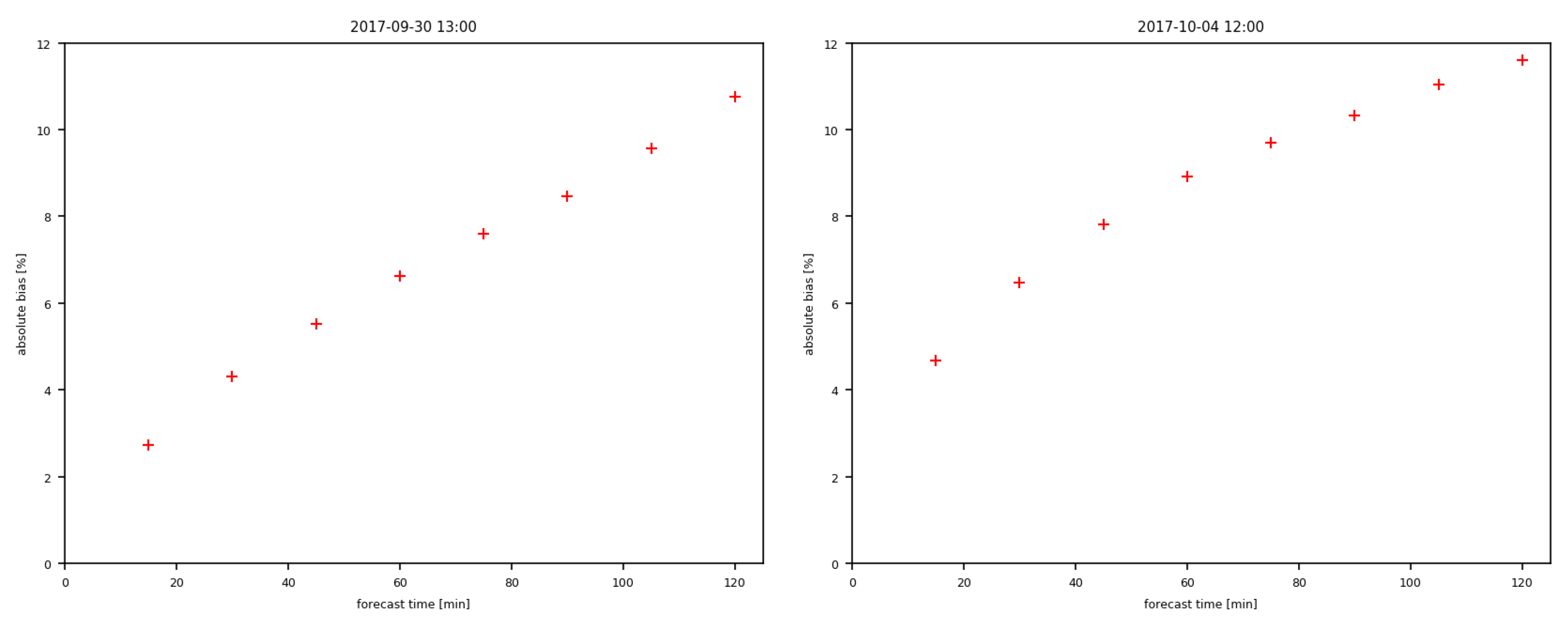
The first task when estimating the optical flow is to change the parameters of the algorithm in a way that the optical flow for the type of data is optimal. For the short-term forecast of solar surface irradiance, we used the effective cloud albedo as the variable for the calculation. To optimize the parameters of the optical flow algorithm, we calculated the bias, absolute bias and RMSE as error measures over the area of Europe (−10–25°N, 36–60°E). The results of the absolute bias for the forecast times from 15 min–120 min are shown in Figure 4. It is shown that the error of the forecast increases non-linearly with the forecast time. The error growth rate decreases with time, which leads to a root-function-shaped graph. This shape can be more or less bent, as can be seen in Figure 4 in the left plot, but the function never reaches linearity.
To choose the optimal value for each parameter of the TV- method, the values had to be changed several times. The optical flow estimate with the parameter value that corresponds to the lowest absolute bias is the most optimal one. However, this is not always as easy as it sounds. For some cases, the parameter values have to be changed for each forecast time. Because this would be difficult to declare for every single case, there should be a better solution. As the differences between a case with optimal and second best values are small, the solution was to calculate the integral of the function seen in Figure 4 with the composite trapezoidal rule to get the overall optimum for the whole forecast. This was done for all 21 cases with a variety of weather situations between August and October 2017 (see Table A1 in the Appendix A). Despite the fact that different weather situations were analyzed, the choice of the parameter values was quite clear, and therefore, it was valid for all short-term forecasts of the effective cloud albedo. Again, the differences of the bias values for optimal and second best parameter values were small, but not negligible. The results of this optimization can be seen in Table 2.
A common approach for numerical models, as well as short-term forecasts is to choose the parameter values in dependence of the spatial scales. In this study, we examined the choice of the parameter value again, but for shorter time periods concerning smaller spatial scales. The result was that the values presented in Table 2 perfectly fit for all forecast times. As can be seen in Figure 4, the plots do not show two or more different regimes, which proves the good choice of the parameters. In other words, the function of the absolute bias against the forecast time is continuous and linearly growing. Moreover, it does not show jumps or features that would differ greatly from the observed shape. The number of cases where this separate choice of parameter values would be successful was too small to be efficiently implemented in the algorithm. On top of that, the achieved effect would be very small.
3.3. One Hundred Twenty-Minute Forecast
In the following subsection, we present two examples of a 120-min forecast based on the optical flow of the effective cloud albedo. The utilized algorithm is DualTVL1OpticalFlow from OpenCV with the parameter values listed in Section 3.2. The two examples were already introduced in the previous subsection.
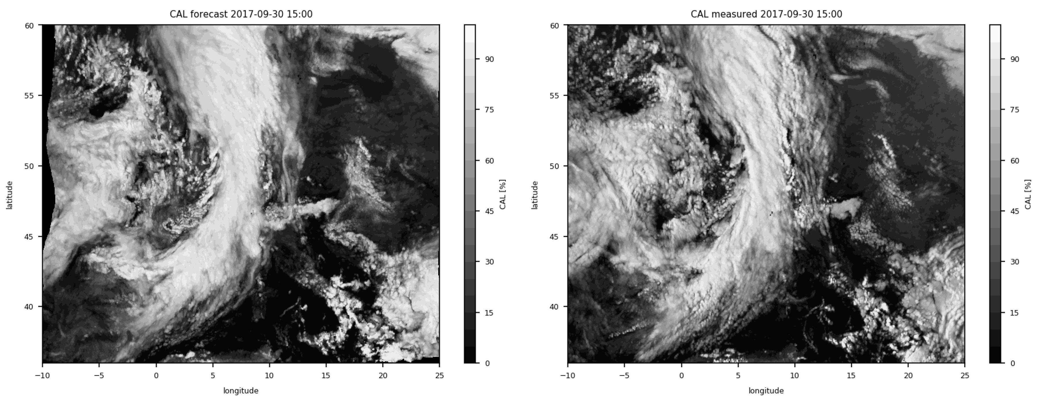
The first case (see Figure 5) shows a quasi-stationary front over Central Europe and post-frontal convective clouds in the west. The front extends from north to south and moves towards the east. Additional convective clouds can be seen over southern Italy and the surrounding ocean.
The forecast figure can be easily recognized by its inward moving edge (Figure 5, left). Due to the given dataset to which the optical flow is added, there is no new information after shifting these cloud pixels to its calculated position. In other words, in an optical flow estimation, all boundary conditions are set to zero. Besides that, the figure depicts a 120-min-forecast, so the clouds usually move further than in a shorter time period. Moreover, the forecast figure can be identified by inspecting the cloud top structure. Due to the fact that a new formation or dissipation of clouds cannot be reproduced with the optical flow estimate, the visual surface structure of the clouds is softer. In the observed satellite image, the cloud tops especially in the area of the front are more structured and show many small details (Figure 5 right). All in all, the position and spatial extent of the cloud formation in the forecast fits quite well to the observations.
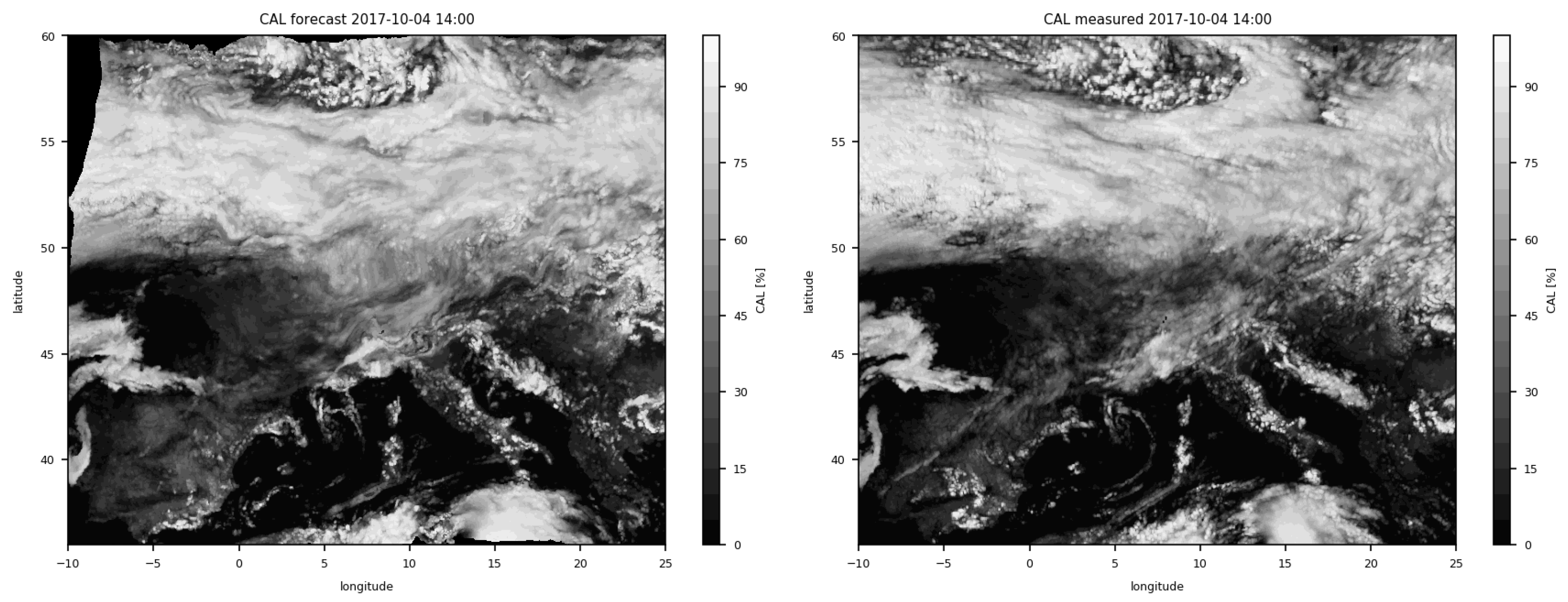
The second case shown here is a different weather situation. Stratiform clouds extend over large parts of Central Europe in the northern part of the chosen area (see Figure 6). Again, convective clouds over southern Italy and the Balkans can be detected. Compared with the observations (Figure 6, right), the surface structure of the simulated cloud area looks quite similar. Nevertheless, the extension to the south is larger in the forecast because over the area of Austria and Switzerland, the clouds dissipated in the time period of 120 min. Furthermore, a few new clouds that cannot be seen in the forecast are formed on the southern tip of Italy.
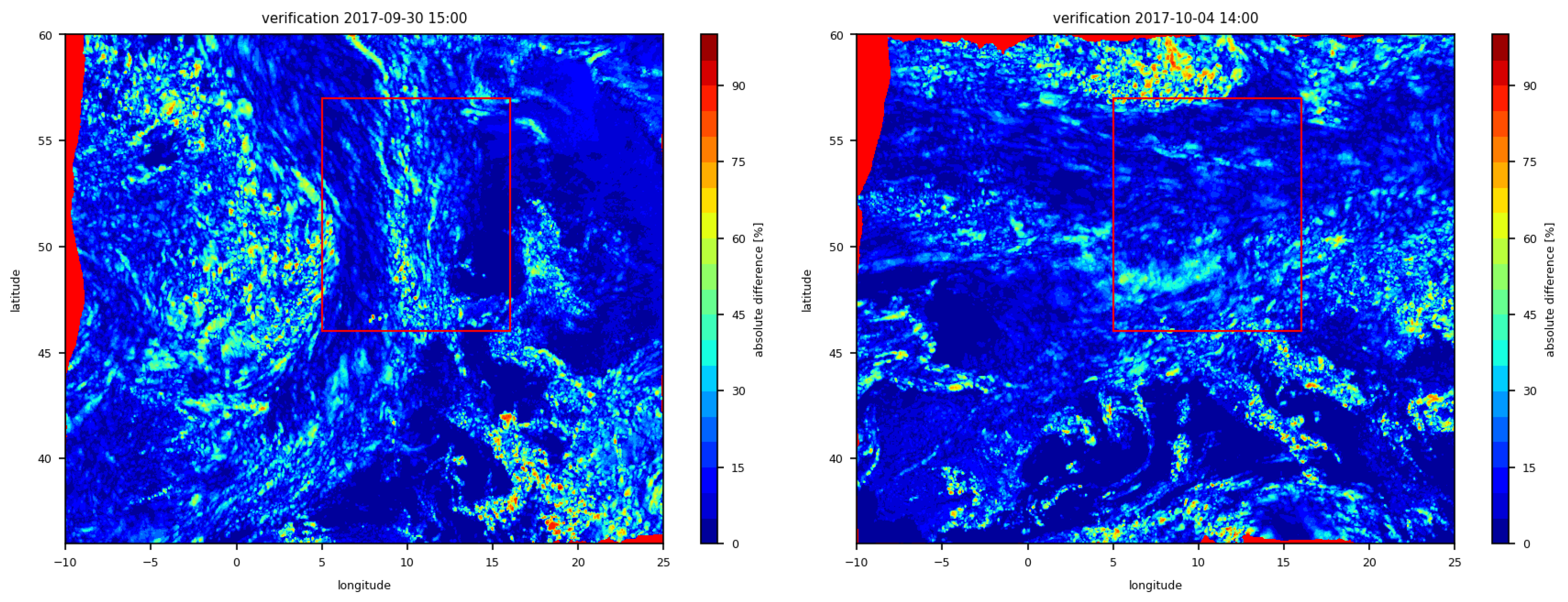
To verify these short-term forecast results of the effective cloud albedo, we calculated the absolute difference between the simultaneous forecast and satellite image. The verification results for the above discussed cases (see Figure 5 and Figure 6) can be seen in Figure 7.
On 30 September, the verification confirms the above-mentioned quality of the forecast. Higher deviations can be seen in areas with the formation of convective clouds, for example over the Mediterranean Sea near the southern tip of Italy or in the area west of the front. Here, the absolute difference can reach values up to 80% in small areas. Moreover, the change of the cloud top structure of the front seems to cause trouble for the algorithm, as well. This can be explained through the changing intensity of each pixel throughout the forecast time. The bias is small for the whole area with 1.98% after 120 min. The other error measures are higher (absolute bias = 12.99%, RMSE = 18.16%) than the bias, which shows that positive and negative deviations are canceled out in the short-term forecast, which is generally the case. All error measures for this case can be found in Table 3.
The bias for the 120-min forecast (bias = 1.84%) is also quite low for 4 October 2017. The other error measures are higher, as well, so that the positive and negative deviations are canceled out, as well (see Table 4). Most of the clouds, especially in the stratiform precipitation area, were forecasted very well, and the verification shows only small deviations. Areas with high absolute differences can be found north of the stratiform clouds and in the south. Both situations can be explained through the formation of new clouds and the changing intensity of cloud pixels. This behavior violates the criterion for the optical flow estimation, which states that the intensity of the pixels has to be constant over time. This is, however, not fulfilled in all cases. Therefore, weather conditions where cloud formation or dissipation occurs pose a problem for the optical flow estimation.
4. Discussion
The applications of optical flow estimates are diverse. As shown in Section 3.3, the utilization of the optical flow estimation for a short-term forecast of the effective cloud albedo and hence of the solar surface irradiance shows promising results. Validation results reported in recent review publications by Voyant et al. [9], Antonanzas et al. [10] or Barbieri et al. [11] and publications by other leading experts (Raza et al. [12], Wolff et al. [1], Cros et al. [33]) do not provide any hints that the application of the widely-used neural networks leads to a significantly better accuracy for cloud motion vectors. In Cros et al. [33], for example, the RMSE of the 30-min forecast of the effective cloud albedo was about 30% for a neural network approach and a phase correlation method. Thus, the discussed optical flow method might be among the best approaches for cloud motion vector estimation. Moreover, the big advantage of the TV- approach, which has been optimized here for the effective cloud albedo, is the free access and the comprehensive documentation of the method. However, no matter which satellite-based method for cloud motion vectors is used, the limit of a good short-term forecast compared to NWP is approximately between 120 and 240 min because the forecast is only based on the optical displacement of pixels. The method does not lead to good forecast results after a certain time threshold. Comparisons with the numerical weather prediction models will be conducted in the future to provide more detailed information about the time when the accuracy of the NWP matches that of TV-. Further, we plan to investigate the benefit of rapid scan imagery, which are available every 5 instead of 15 min.
A currently known problem of satellite imagery methods is the formation or dissipation of clouds in the forecast, which can be caused for example by fast processes such as convection. This is confirmed by our verification results (see Figure 7). As mentioned above, one criterion of the optical flow is that the intensity of image pixels has to stay constant between two consecutive frames. Due to the fact that convective clouds form very fast, this is clearly not fulfilled. Nevertheless, these areas where convection can be found are very small in comparison to stratiform clouds or fronts and, thus, are rather negligible for renewable energy forecasts. A common approach for short-term forecasts is the separation into sub-scales. Convection is a fast small-scale process, while pressure systems with fronts can extend up to 1000 km and exist for days. To cover both regimes, the optimization process can be done for the first 60 min and the second 60 or more minutes. This was already conducted for the 21 cases mentioned, but it did not improve the forecast. From 21 cases, there were only four in which a separate optimization would be useful. Besides, the differences between the optimal and the second best parameter value are in the range of hundredths and thus negligible. The implementation of such a parameter change would just be too costly.
5. Conclusions
The demand for more precise short-term forecasts for wind and solar irradiance over shorter time horizons is growing as a consequence of the increasing use of renewable energies. A short-term forecast of solar surface irradiance can be obtained via optical flow estimation of the effective cloud albedo. For this purpose, we used the TV- algorithm by Zach et al. available from OpenCV [2,28]. As is shown in Figure 3 and Table 1, the method by Zach et al. for the estimation of the optical flow delivers better results than the method by Farnebäck, a short-term forecast of the effective cloud albedo. The presented experiments show that the use of TV- for the estimation of the optical flow works well for the short-term forecast of the effective cloud albedo and thus for the solar surface irradiance. Due to the high temporal and spatial resolution of satellite measurements, the short-term forecast of solar surface irradiance can cover a period of 5 min up to 4 h with a spatial resolution of 0.05°. The calculated RMSE for the 30-min, 60-min, 90-min and 120-min forecast equals 10.47%, 14.28%, 16.87% and 18.83%, respectively (see Table A2 in the Appendix A for more error measures). Overall, the error measures are small for the examined cases, although the formation and dissipation of clouds pose problems for the optical flow estimation in general. One of the major assumptions for the optical flow estimation is that the intensity of pixels remains similar between two consecutive time frames. However, this is not fulfilled when new clouds occur or grow. This is the case because the newly-formed top of the cloud consists of smaller droplets, and thus, the effective cloud albedo is higher because more light is reflected. Moreover, larger clouds or clouds at other positions can be formed in the time between the two frames. Nevertheless, these issues normally take place on small scales and do not influence the regional forecast too much. In general, the results show that the approach is very promising.
Author Contributions
I.U. optimized the optical flow estimation and performed the validation. R.M. developed the approach for the retrieval of the effective cloud albedo and the clear-sky model SPECMAGIC. J.B. participated as the mentor of the work. All authors contributed to the writing of the manuscript.
Acknowledgments
We thank Manuel Werner and Stephane Haussler for sharing their experience in optical flow estimation with us. Thanks to Markus Kunert, Michael Mott, Nils Rathmann and Manuel Werner for the introduction and support regarding the POLARA framework, which was developed by the department of radar meteorology at the German Weather Service. We also thank Matthias Jerg for the cross-reading of the manuscript.
Conflicts of Interest
The authors declare no conflict of interest.
Abbreviations
| CAL | Effective cloud albedo |
| Cb-TRAM | Tracking and monitoring severe convection from onset over rapid development to mature phase using multi-channel Meteosat-8 SEVIRI data |
| CMSAF | Climate Monitoring Satellite Application Facility |
| EUMETSAT | European Organisation for the Exploitation of Meteorological Satellites |
| HRV | High resolution visible |
| MFG | Meteosat First Generation |
| MSG | Meteosat Second Generation |
| Meteosat | Meteorological Satellite |
| MVIRI | Meteosat Visible and Infrared Imager |
| NN | Neural networks |
| NWCSAF | Nowcasting Satellite Application Facility |
| NWP | Numerical weather prediction model |
| OpenCV | Open Source Computer Vision |
| POLARA | Polarimetric radar algorithms |
| PV | Photovoltaic |
| RMSE | Root mean square error |
| SEVIRI | Spinning Enhanced Visible and Infrared Imager |
| SSI | Solar surface irradiance |
| TV- | Method based on total variation in the regularization term and the -norm in the data fidelity term |
Appendix A

Table A1.
List of investigated cases for the settings of the parameters in the TV- method for the optical flow estimation of the effective cloud albedo. The error measures were calculated for a 15-min-forecast over the area of Europe.
Table A1.
List of investigated cases for the settings of the parameters in the TV- method for the optical flow estimation of the effective cloud albedo. The error measures were calculated for a 15-min-forecast over the area of Europe.
| Day | Time | Weather Situation | Bias (%) | Absolute Bias (%) | RMSE (%) |
|---|---|---|---|---|---|
| 7 August 2017 | 09:00 | high pressure | −0.61 | 3.06 | 5.49 |
| 11 August 2017 | 14:00 | stratiform precipitation | 0.82 | 4.32 | 7.76 |
| 15:00 | stratiform precipitation | 0.06 | 4.31 | 7.69 | |
| 16:00 | stratiform precipitation | −0.21 | 4.80 | 8.21 | |
| 15 August 2017 | 14:00 | convection | 0.51 | 3.66 | 6.86 |
| 15:00 | convection | 0.07 | 3.63 | 6.78 | |
| 28 August 2017 | 15:00 | high pressure | 0.04 | 4.77 | 8.23 |
| 29 August 2017 | 12:00 | high pressure | 0.08 | 3.90 | 7.03 |
| 1 September 2017 | 12:00 | stratiform precipitation | 0.10 | 3.52 | 6.40 |
| 7 September 2017 | 15:00 | broken clouds | 0.53 | 4.61 | 7.19 |
| 17 September 2017 | 12:00 | broken clouds | 0.24 | 4.71 | 8.24 |
| 19 September 2017 | 14:00 | broken clouds | 1.69 | 5.73 | 9.37 |
| 22 September 2017 | 09:00 | broken clouds | 0.36 | 3.92 | 6.65 |
| 26 September 2017 | 12:00 | convection | 0.44 | 4.67 | 7.68 |
| 13:00 | convection | 0.31 | 4.80 | 7.82 | |
| 30 September 2017 | 13:00 | front & convection | 0.10 | 4.08 | 6.67 |
| 1 October 2017 | 09:00 | front | 0.41 | 4.13 | 6.48 |
| 2 October 2017 | 12:00 | stratiform precipitation | 0.33 | 4.83 | 8.06 |
| 3 October 2017 | 13:00 | broken clouds | 0.21 | 5.28 | 8.35 |
| 4 October 2017 | 12:00 | stratiform precipitation | 0.44 | 4.22 | 9.57 |
| 7 October 2017 | 10:00 | stratiform precipitation | −0.31 | 4.47 | 7.78 |
Table A2.
Mean values of the bias, absolute bias and RMSE for all investigated cases. The basis for the calculation is the area of Europe.
Table A2.
Mean values of the bias, absolute bias and RMSE for all investigated cases. The basis for the calculation is the area of Europe.
| Forecast Time (Min) | Bias (%) | Absolute Bias (%) | RMSE (%) |
|---|---|---|---|
| 30 | 0.41 | 6.35 | 10.47 |
| 60 | 0.41 | 9.10 | 14.28 |
| 90 | 0.57 | 11.12 | 16.87 |
| 120 | 0.43 | 12.78 | 18.83 |
References
- Wolff, B.; Kühnert, J.; Lorenz, E.; Kramer, O.; Heinemann, D. Comparing support vector regression for PV power forecasting to a physical modeling approach using measurement, numerical weather prediction, and cloud motion data. Sol. Energy 2016, 135, 197–208. [Google Scholar] [CrossRef]
- OpenCV Homepage. Available online: http://opencv.org/ (accessed on 11 January 2018).
- Sonka, M.; Hlavac, V.; Roger, B. Image Processing, Analysis, and Machine Vision, International Edition; Cengage Learning: Boston, MA, USA, 2014; ISBN -13-978-1-133-59360-7. [Google Scholar]
- Peura, M.; Hohti, H. Optical flow in radar images. In Proceedings of the Third European Conference on Radar Meteorology (ERAD) Together with the COST 717 Final Seminar, Visby, Island of Gotland, Sweden, 6–10 September 2004; pp. 454–458. [Google Scholar]
- Mueller, R.; Trentmann, J.; Träger-Chatterjee, C.; Posselt, R.; Stöckli, R. The Role of the Effective Cloud Albedo for Climate Monitoring and Analysis. Remote Sens. 2011, 3, 2305–2320. [Google Scholar] [CrossRef] [Green Version]
- Rosenow, R.; Güldner, J.; Spänkuch, D. The Satellite Weather of the German Weather Service—An assimilation procedure with a spectral component. In Proceedings of the 2001 EUMETSAT Meteorological Satellite Data User’s Conference, Antalya, Turkey, 1–5 October 2001; pp. 541–545. [Google Scholar]
- Schmetz, J.; Holmlund, K.; Hoffman, J.; Strauss, B.; Mason, B.; Gaertner, V.; Koch, A.; Berg, L.V.D. Operational Cloud-Motion Winds from Meteosat Infrared Images. J. Appl. Meteorol. 1993, 32, 1206–1225. [Google Scholar] [CrossRef] [Green Version]
- García Pereda, J. Algorithm Theoretical Basis Document for the Wind Product Processors of the NWC/GEO. SAF-ATBD: NWC/CDOP2/GEO/AEMET/SCI/ATBD/Wind, NWC-SAF. 2016. Available online: http://www.nwcsaf.org/documents/20182/30801/NWC-CDOP2-GEO-AEMET-SCI-ATBD-Wind_v1.1.pdf (accessed on 15 June 2015).
- Voyant, C.; Notton, G.; Kalogirou, S.; Nivet, M.L.; Paoli, C.; Motte, F.; Fouilloy, A. Machine learning methods for solar radiation forecasting: A review. Renew. Energy 2017, 105, 569–582. [Google Scholar] [CrossRef]
- Antonanzas, J.; Osorio, N.; Escobar, R.; Urraca, R.; Martinez-de Pison, F.; Antonanzas-Torres, F. Review of photovoltaic power forecasting. Sol. Energy 2016, 136, 78–111. [Google Scholar] [CrossRef]
- Barbieri, F.; Rajakaruna, S.; Gosh, A. Very short-term photovoltaic power forecasting with cloud modeling: A review. Renew. Sustain. Energy Rev. 2017, 75, 242–263. [Google Scholar] [CrossRef]
- Raza, M.Q.; Nadarajah, M.; Ekanayake, C. On recent advances in PV output power forecast. Sol. Energy 2016, 136, 125–144. [Google Scholar] [CrossRef]
- Perez, R.; Kankiewicz, A.; Schlemmer, J.; Hemker, K.; Kivalov, S. A new operational solar resource forecast model service for PV fleet simulation. In Proceedings of the Photovoltaic Specialist Conference (PVSC), Denver, CO, USA, 8–13 June 2014; pp. 0069–0074. [Google Scholar]
- Aksakal, S. Geometric Accuracy Investigations of SEVIRI High Resolution Visible (HRV) Level 1.5 Imagery. Remote Sens. 2013, 5, 2475–2491. [Google Scholar] [CrossRef] [Green Version]
- Simonenko, E.; Chudin, A.O.; Davidenko, A. The Differential Method for Calculation of Cloud Motion Vectors. Russ. Meteorol. Hydrol. 2017, 42, 159–167. [Google Scholar] [CrossRef]
- Sirch, T.; Bugliaro, L.; Zinner, T.; Möhrlein, M.; Vazquez-Navarro, M. Cloud and DNI nowcasting with MSG/SEVIRI for the optimized operation of concentrating solar power plants. Atmos. Meas. Tech. 2017, 10, 409–429. [Google Scholar] [CrossRef] [Green Version]
- Zinner, T.; Mannstein, H.; Tafferner, A. Cb-TRAM: Tracking and monitoring severe convection from onset over rapid development to mature phase using multiple-channel Meteosat-8 SEVIRI data. Meteorol. Atmos. Phys. 2008, 101, 191–210. [Google Scholar] [CrossRef] [Green Version]
- Zinner, T.; Forster, C.; de Coning, E.; Betz, H.D. Validation of the Meteosat storm detection and nowcasting system Cb-TRAM with lightning network data—Europe and South Africa. Atmos. Meas. Tech. 2013, 6, 1567–1583. [Google Scholar] [CrossRef] [Green Version]
- Mueller, R.; Behrendt, T.; Hammer, A.; Kemper, A. A New Algorithm for the Satellite-Based Retrieval of Solar Surface Irradiance in Spectral Bands. Remote Sens. 2012, 4, 622–647. [Google Scholar] [CrossRef] [Green Version]
- Burton, A.; Radford, J. Thinking in Perspective: Critical Essays in the Study of Thought Processes; Psychology in Progress: Methuen, MA, USA, 1978. [Google Scholar]
- Beauchemin, S.S.; Barron, J.L. The computation of optical flow. ACM Comput. Surv. (CSUR) 1995, 27, 433–466. [Google Scholar] [CrossRef] [Green Version]
- Barron, J.L.; Fleet, D.J.; Beauchemin, S.S. Performance of optical flow techniques. Int. J. Comput. Vis. 1994, 12, 43–77. [Google Scholar] [CrossRef] [Green Version]
- Pérez, J.S.; Meinhardt-Llopis, E.; Facciolo, G. TV-L1 Optical Flow Estimation. Image Process. Line 2013, 3, 137–150. [Google Scholar] [CrossRef] [Green Version]
- Horn, B.K.; Schunck, B.G. Determining optical flow. Artif. Intell. 1981, 17, 185–203. [Google Scholar] [CrossRef] [Green Version]
- Baker, S.; Scharstein, D.; Lewis, J.; Roth, S.; Black, M.J.; Szeliski, R. A database and evaluation methodology for optical flow. Int. J. Comput. Vis. 2011, 92, 1–31. [Google Scholar] [CrossRef]
- Zhang, G.; Chanson, H. Application of local optical flow methods to high-velocity free-surface flows: Validation and application to stepped chutes. Exp. Therm. Fluid Sci. 2018, 90, 186–199. [Google Scholar] [CrossRef] [Green Version]
- Farnebäck, G. Two-frame motion estimation based on polynomial expansion. Image Anal. 2003, 2749, 363–370. [Google Scholar]
- Zach, C.; Pock, T.; Bischof, H. A Duality Based Approach for Realtime TV-L1 Optical Flow. In Proceedings of the 29th DAGM Symposium, Pattern Recognition, Heidelberg, Germany, 12–14 September 2007; pp. 214–223. [Google Scholar]
- Cano, D.; Monget, J.; Albuisson, M.; Guillard, H.; Regas, N.; Wald, L. A method for the determination of the global solar radiation from meteorological satellite data. Sol. Energy 1986, 37, 31–39. [Google Scholar] [CrossRef] [Green Version]
- Beyer, H.; Costanzo, C.; Heinemann, D. Modifications of the Heliosat procedure for irradiance estimates from satellite images. Sol. Energy 1996, 56, 207–212. [Google Scholar] [CrossRef]
- Hammer, A.; Heinemann, D.; Hoyer, C.; Kuhlemann, R.; Lorenz, E.; Mueller, R.; Beyer, H. Solar Energy Assessment Using Remote Sensing Technologies. Remote Sens. Environ. 2003, 86, 423–432. [Google Scholar] [CrossRef]
- Chambolle, A. An Algorithm for Total Variation Minimization and Applications. J. Math. Imaging Vis. 2004, 20, 89–97. [Google Scholar] [CrossRef]
- Cros, S.; Liandrat, O.; Sébastien, N.; Schmutz, N. Extracting cloud motion vectors from satellite images for solar power forecasting. In Proceedings of the 2014 IEEE Geoscience and Remote Sensing Symposium, Quebec City, QC, Canada, 13–18 July 2014; pp. 4123–4126. [Google Scholar]
Figure 1.
Scheme of the optical flow method. Two images of the effective cloud albedo serve as input for the TV- method. The estimated cloud motion vectors are then applied to the latter of the consecutive images to extrapolate the cloud motion into the future.
Figure 1.
Scheme of the optical flow method. Two images of the effective cloud albedo serve as input for the TV- method. The estimated cloud motion vectors are then applied to the latter of the consecutive images to extrapolate the cloud motion into the future.

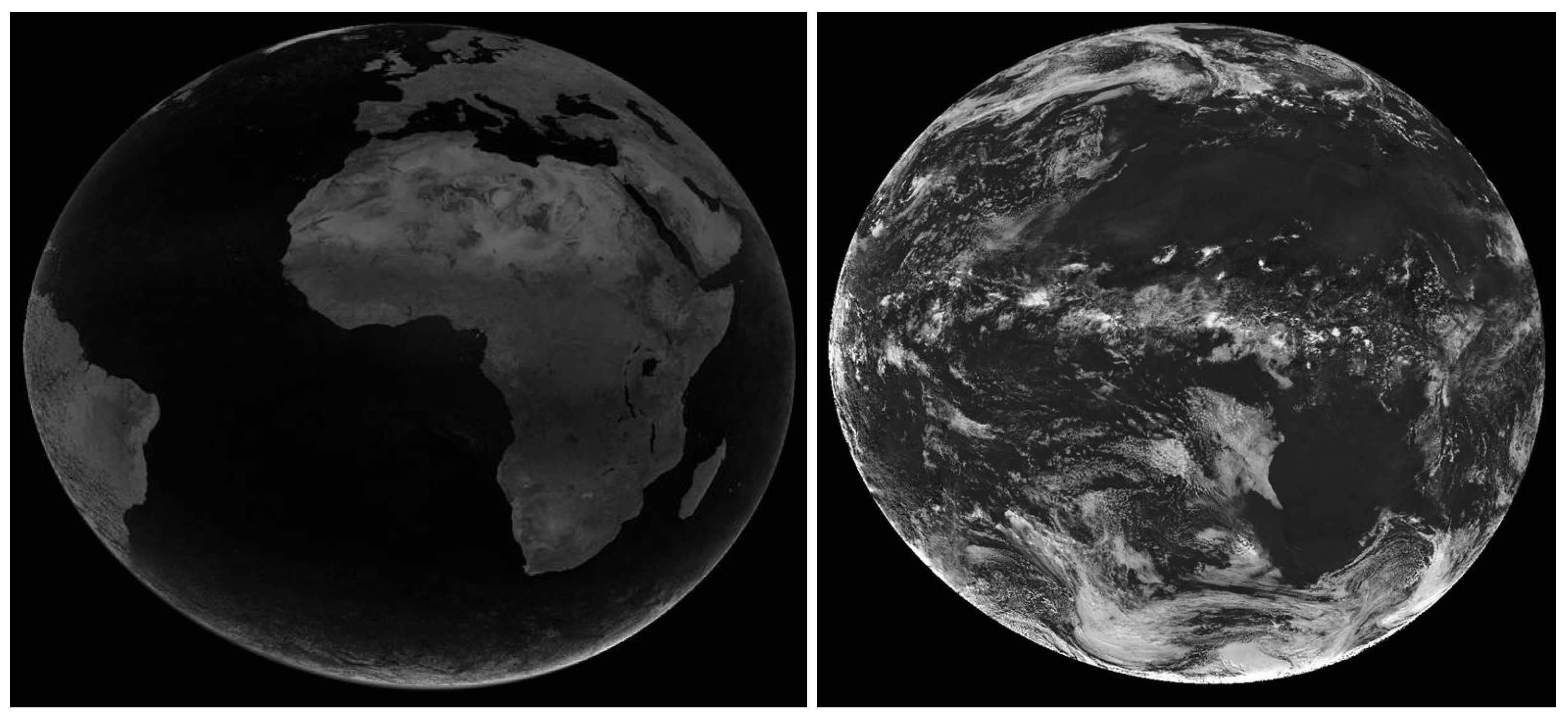
Figure 2.
Example of the clear sky reflection (left) and effective cloud albedo CAL (right) for an 11 UTC slot in June 2005.
Figure 2.
Example of the clear sky reflection (left) and effective cloud albedo CAL (right) for an 11 UTC slot in June 2005.

Figure 3.
Plots of the verification of the optical flow estimate with the method by Farnebäck (left) and the TV- method (right) for a 15-min forecast. The area of Germany is marked by the red frame.
Figure 3.
Plots of the verification of the optical flow estimate with the method by Farnebäck (left) and the TV- method (right) for a 15-min forecast. The area of Germany is marked by the red frame.

Figure 4.
Plots of the absolute bias of the effective cloud albedo against the forecast time for the cases of 30 September 2017 at 13:00 UTC (situation with convection behind a front over Germany) and 4 October 2017 at 12:00 UTC (stratiform situation). The unit of the absolute bias is %.
Figure 4.
Plots of the absolute bias of the effective cloud albedo against the forecast time for the cases of 30 September 2017 at 13:00 UTC (situation with convection behind a front over Germany) and 4 October 2017 at 12:00 UTC (stratiform situation). The unit of the absolute bias is %.

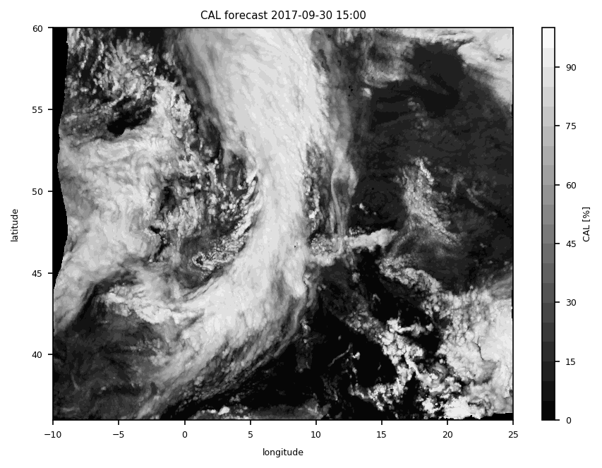
Figure 5.
A short-term forecast for 120 min of the effective cloud albedo for 30 September 2017 at 15:00 UTC can be seen in the left figure. The satellite image by MSG with the effective cloud albedo depicted for comparison is shown in the right image.
Figure 5.
A short-term forecast for 120 min of the effective cloud albedo for 30 September 2017 at 15:00 UTC can be seen in the left figure. The satellite image by MSG with the effective cloud albedo depicted for comparison is shown in the right image.

Figure 6.
A short-term forecast for 120 min of the effective cloud albedo for 4 October 2017 at 14:00 UTC can be seen in the left figure. The satellite image by MSG with the effective cloud albedo depicted for comparison is shown in the right image.
Figure 6.
A short-term forecast for 120 min of the effective cloud albedo for 4 October 2017 at 14:00 UTC can be seen in the left figure. The satellite image by MSG with the effective cloud albedo depicted for comparison is shown in the right image.

Figure 7.
Verification plots of the optical flow method for the cases of 30 September 2017 at 15:00 UTC and 4 October 2017 at 14:00 UTC. The absolute difference between the effective cloud albedo from satellite imagery and the effective cloud albedo from the short-term forecast for 120 min in % is shown.

Table 1.
Calculated absolute bias and RMSE for both optical flow methods, the one by Farnebäck and with TV-. The error measures were calculated for a 15-min forecast over the area of Europe. These are 10 exemplary cases because the superiority of TV- can be clearly seen already, and these values are sufficient to see the difference between the performance of the methods.
| Day | Time | Farnebäck | TV- | ||
|---|---|---|---|---|---|
| abs. bias (%) | RMSE (%) | abs. bias (%) | RMSE (%) | ||
| 7 August 2017 | 09:00 | 5.07 | 9.19 | 3.87 | 7.03 |
| 11 August 2017 | 15:00 | 7.4 | 12.81 | 5.54 | 9.81 |
| 15 August 2017 | 15:00 | 6.67 | 12.22 | 4.83 | 8.96 |
| 1 September 2017 | 12:00 | 6.36 | 11.29 | 4.67 | 8.46 |
| 17 September 2017 | 12:00 | 5.43 | 9.53 | 4.37 | 7.59 |
| 22 September 2017 | 09:00 | 6.82 | 11.24 | 5.25 | 8.82 |
| 30 September 2017 | 13:00 | 7.19 | 11.68 | 5.31 | 8.75 |
| 1 October 2017 | 09:00 | 7.25 | 11.19 | 5.57 | 8.73 |
| 3 October 2017 | 13:00 | 9.34 | 14.76 | 6.79 | 10.78 |
| 4 October 2017 | 12:00 | 7.62 | 12.18 | 5.94 | 9.57 |
Table 2.
List of parameter settings for the TV- method in the DualTVL1OpticalFlow algorithm by OpenCV.
Table 2.
List of parameter settings for the TV- method in the DualTVL1OpticalFlow algorithm by OpenCV.
| Parameter | Value | Parameter | Value |
|---|---|---|---|
| 0.1 | outer iterations | 2 | |
| 0.1 | inner iterations | 10 | |
| 0.03 | 3 | ||
| 0.3 | 3 | ||
| 0.01 | scale step | 0.5 |
Table 3.
Values of the bias, absolute bias and RMSE for the case of 30 September 2017. The basis for the calculation is the area of Europe.
Table 3.
Values of the bias, absolute bias and RMSE for the case of 30 September 2017. The basis for the calculation is the area of Europe.
| forecast Time (Min) | Bias (%) | Absolute Bias (%) | RMSE (%) |
|---|---|---|---|
| 30 | 0.11 | 5.95 | 9.49 |
| 60 | −0.37 | 8.68 | 13.40 |
| 90 | 1.55 | 10.77 | 15.77 |
| 120 | 1.98 | 12.99 | 18.16 |
Table 4.
Values of the bias, absolute bias and RMSE for the case of 4 October 2017. The basis for the calculation is the area of Europe.
Table 4.
Values of the bias, absolute bias and RMSE for the case of 4 October 2017. The basis for the calculation is the area of Europe.
| Forecast Time (Min) | Bias (%) | Absolute Bias (%) | RMSE (%) |
|---|---|---|---|
| 30 | 0.85 | 6.02 | 9.57 |
| 60 | 1.48 | 8.24 | 12.85 |
| 90 | 1.93 | 9.61 | 14.69 |
| 120 | 1.84 | 10.78 | 16.21 |
© 2018 by the authors. Licensee MDPI, Basel, Switzerland. This article is an open access article distributed under the terms and conditions of the Creative Commons Attribution (CC BY) license (http://creativecommons.org/licenses/by/4.0/).
Share and Cite
MDPI and ACS Style
Urbich, I.; Bendix, J.; Müller, R. A Novel Approach for the Short-Term Forecast of the Effective Cloud Albedo. Remote Sens. 2018, 10, 955. https://0-doi-org.brum.beds.ac.uk/10.3390/rs10060955
AMA Style
Urbich I, Bendix J, Müller R. A Novel Approach for the Short-Term Forecast of the Effective Cloud Albedo. Remote Sensing. 2018; 10(6):955. https://0-doi-org.brum.beds.ac.uk/10.3390/rs10060955
Chicago/Turabian StyleUrbich, Isabel, Jörg Bendix, and Richard Müller. 2018. "A Novel Approach for the Short-Term Forecast of the Effective Cloud Albedo" Remote Sensing 10, no. 6: 955. https://0-doi-org.brum.beds.ac.uk/10.3390/rs10060955
Note that from the first issue of 2016, this journal uses article numbers instead of page numbers. See further details here.