Bayesian Bias Correction of Satellite Rainfall Estimates for Climate Studies


Faculty of Geo-Information Science and Earth Observation, University of Twente, 217 7500 AE Enschede, The Netherlands
*
Author to whom correspondence should be addressed.
Remote Sens. 2018, 10(7), 1074; https://0-doi-org.brum.beds.ac.uk/10.3390/rs10071074
Submission received: 16 April 2018
/
Revised: 28 June 2018
/
Accepted: 2 July 2018
/
Published: 5 July 2018
(This article belongs to the Special Issue Advancing Earth Surface Representation via Enhanced Use of Earth Observations in Monitoring and Forecasting Applications)
Abstract
:Advances in remote sensing have led to the use of satellite-derived rainfall products to complement the sparse rain gauge data. Although these products are globally and some regional bias corrected, they often show substantial differences relative to ground measurements attributed to local and external factors that require systematic consideration. A decreasing rain gauge network inhibits the continuous validation of these products. Our proposal to deal with this problem was to use a Bayesian approach to merge the existing historical rain gauge information to create consistent satellite rainfall data for long-term applications. Monthly bias correction was applied to Climate Hazards Group Infrared Precipitation with Stations (CHIRPS v2) using a corresponding gridded (0.05°) rain gauge data over East Africa for 33 years (1981–2013). The first 22 years were utilized to derive error fields which were then applied to independent CHIRPS data for 11 years for validation. Assessments of the approach’s influence on the rainfall estimates spatially and temporally were explored. Results showed a significant spatial reduction of the underestimation and overestimation of systematic errors at both monthly and yearly scales. The reduced errors increased with increased rainfall amounts, hence was less so in the relatively drier months. The overall monthly reduction of Root Mean Square Difference (RMSD) was between 4% and 60%, and the Mean Absolute Error (MAE) was between 1% and 63%, while the correlations improved by up to 21%. Yearly, the RMSD was reduced between 17% and 49%, and the MAE between 13% and 48%, while the increase in correlations was between 9% and 17%. Decreased yearly bias correction corresponded with years of high rainfall associated with El Niño. Results for the assessments of the effectiveness of the Bayesian approach showed that it was more effective in reducing systematic errors related to rainfall magnitudes, but its performance decreased in areas of sparse rain gauge network that insufficiently represented rainfall variabilities. This affected areas of deep convection, leading to minimal overestimation reductions associated with the cirrus effect. Conversely, significant corrections were during years of low rainfall from shallow convections. The approach is suitable for long-term applications where consistencies of mean errors can be assumed.
1. Introduction
Rainfall data is vital for many applications such as climate studies, water resource management, and agriculture. As its accurate spatial and temporal representations can improve socio-economic planning. Rain gauges provide the most direct representations of rainfall, but their distribution over land are sparse, especially in mountainous areas [1], and being point observations, they lack spatial representativeness [2]. However, they offer useful information in modelling regarding local rainfall processes that are not accurately parameterized by the Global Circulation Models (GCM) [3]. Alternative uses of satellite rainfall products are increasing because of their high spatiotemporal coverage. However, these products often exhibit large discrepancies with ground measurements [4,5], and the errors need to be reduced to make the products more representative of the local rainfall variability. Although some of these products are globally validated [6,7,8] and some at regional scales [9,10], relatively few efforts have been made to reduce the often-large errors that occur at local scales. Studies [11,12,13] have found that satellite rainfall products have systematic errors that cause overestimations/underestimations, especially in high elevated areas [13]. Although rain gauge data have low spatial distributions, their direct way of measuring rainfall are still vital as a reference to the local rainfall variability. For better representations of local rainfall processes, the inclusion of all available quality controlled rain gauge data merged with satellite products can enhance the products’ future applications. Different methods have been proposed to reduce satellite rainfall estimates errors. A study by [12] applied bias correction using empirical cumulative distribution (CDF) maps on a seasonal basis for hydrological applications in the upper Blue Nile in Ethiopia. To reduce temporal rainfall variability, a seasonal timescale was utilized. However, in high elevated areas, areas near inland water bodies, and those with maritime influences, high rainfall variabilities are experienced. As such, the choice of temporal scale may differ from place to place. It is worth noting that the effectiveness of bias correction on rainfall products may also differ from location to location and consideration of spatial scale is of great importance. Quantile mapping approach was applied by [14] to bias correct rainfall products and they observed that the approach improved estimates in some locations, while it degraded in others. However, it is crucial that the applied method does not necessarily change the product’s original rainfall estimates. Therefore, the consistencies of the systematic errors corrected are worthy of consideration. Mateus et al. [15] assessed the performance of two bias correction methods—successive correction method (SCM) and optimal interpolation and qualitative analysis—and visual inspections showed better results by SCM. However, the study noted the limitation of this approach in defining the optimal weight of the error distributions. Elsewhere, ref. [16] evaluated satellite rainfall estimates combined with high-resolution rain gauge data using different bias correction methods based on an additive, multiplicative, and merged scheme approach. The evaluation was carried out on a monthly basis in different rainfall seasons and with different rain gauge networks. The results revealed that the choice of both the temporal and spatial scale of the rain gauge data was vital for adequate bias correction. In their study, the merged scheme showed the best results. Nevertheless, this approach is more suitable for real-time applications and in many areas of the world, the degradation of the rain gauge network is a common problem due to the lack of maintenance. Furthermore, for climate studies and other long-term applications, real-time data is not applicable.
A probabilistic Bayesian approach was applied by [17] on high temporal resolution rain gauge data. Historical rain gauge and satellite data were used to create a satellite estimates–rain gauge data relationship, which is applicable in the absence of real-time rain gauge data. The approach worked well even in areas of low rain gauge distributions, but over corrections were observed in some areas. However, it is understandable that rainfall variability differs from place to place and the impact of rain gauge distribution needs to be determined. It is a fact that over the world, rain gauge distributions are decreasing [18], especially in African countries due to their cost of maintenance. Their availabilities to validate the increasing satellite rainfall products may be affected by inconsistencies caused by the low network. Despite this, they offer useful information on the local rainfall variabilities. Over equatorial East Africa, few studies like [19] have used high-resolution ground data to bias-correct satellite rainfall estimates for hydrological applications. It is crucial to have long-term bias correction because of the accumulation of errors in time and for externally induced errors, particularly in areas that experience high rainfall variability [13].
We proposed a Bayesian approach that could be used with the existing historical rain gauge information to create consistent satellite rainfall data for long-term applications. This approach assumes consistencies in time for the average errors in both datasets. As such, the error weight derived from their climatology is considered to be representative of a given area. In our approach, we converted the probability into independent variables to apply a linear relationship using the least square techniques [20]. This approach is superior to other methods in that it does not always modify the estimates during corrections, but considers the mean error consistencies of the input data in time. Therefore, the corrected satellite estimates approach the uncorrected state in areas of poor rainfall representations arising from sparse rain gauge distribution. This way, the satellite rainfall estimates remain close to the original state in areas of inconsistent rain gauge data. A long-term (1981–2013) temporal scale bias correction was applied to the Climate Hazards Group Infrared Precipitation with Stations (CHIRPS v2). The product was chosen based on its high spatial resolution and lengthy climatology suitable for climate studies to help end users in planning [21]. Furthermore, a recent study by [13] over East Africa showed a close correspondence of CHIRPS v2, Tropical Rainfall Measuring Mission (TRMM)3B43, and the Climate Prediction Center (CPC) morphing technique (CMORPH) with ground observations. However, in that study, all the satellite products assessed exhibited large biases in high elevated areas. Although CHIRPS is globally bias corrected using some of the rain gauge data used in this study, the data mainly come from the Global Telecommunication System (GTS). The GTS stations are sparse and may therefore not accurately represent the rainfall variability over the region.
This study assessed the performance of the Bayesian approach in reducing systematic errors on CHIRPS v2 rainfall estimates relative to regional gridded rain gauge data. The assessments on the effectiveness of the method were on a monthly and yearly basis. This paper has six sections. Section 1 presents the introduction; Section 2 gives a brief description of the study area and data used, Section 3 describes the Bayesian approach and methods of evaluation; Section 4 presents the results, discussions of the results are in Section 5 while our conclusions are in Section 6.
2. Study Region and Data
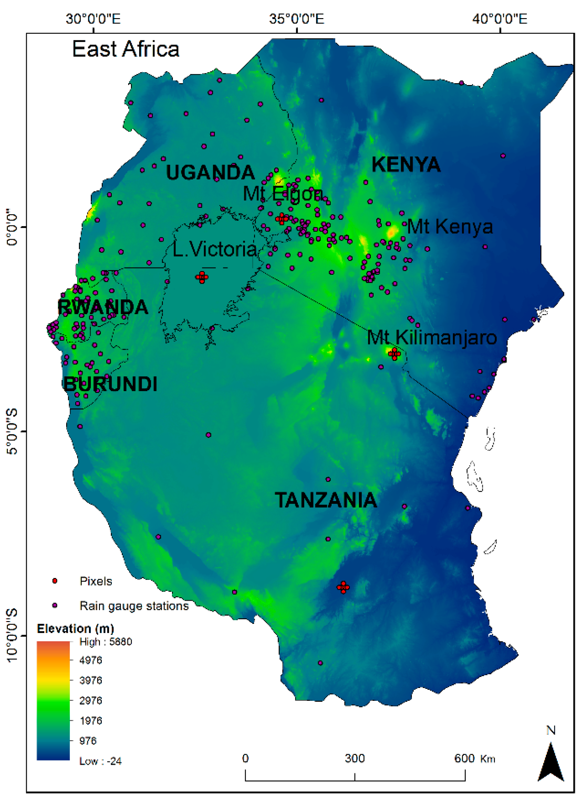
The study area in East Africa (Figure 1) extended between 29°E and 42°E, and 12°S and 5°N and covered five countries: Kenya, Uganda, Tanzania, Burundi, and Rwanda. The region shows diverse topography delineated by the embedded elevation map. Two main rainy seasons occur during March, April, and May (MAM) and October, November, and December (OND). These rainy seasons coincide with the overlying of a low-pressure belt of the Inter-Tropical Convergence Zone (ITCZ). The ITCZ migrates from 15°S to 15°N between January and July with characteristics of convective activities that lead to increased precipitation. A third rainfall season occurs in the months of June through to August (JJA) and affects a small part of Western Kenya and Uganda. This season significantly affects water resources within the region and areas around Lake Victoria.
Two monthly rainfall datasets were used in this study and included CHIRPS v2 rainfall estimates and rain gauge data. CHIRPS is a quasi-global dataset developed by the United States Geological Survey (USGS) Earth Resources Observations and Science Centre and the University of California Santa Barbara Climate Hazards Group. It has a spatial resolution of 0.05°, and a daily/pentad/monthly temporal resolution. It uses TRMM multi-satellite precipitation analysis version 7 to calibrate the Cold Cloud Duration (CCD) rainfall estimates. The product covers the area between 50°N and 50°S, and data are available from January 1981 to the near present. Further details of CHIRPS v2 used in this study can be found in [22], and an evaluation of its performance relative to other products in [10].
The gridded (0.05°) rain gauge was from the Intergovernmental Authority on Development (IGAD) Climate Prediction and Application Centre (ICPAC [23]. Although the data includes global telecommunication stations, ICPAC includes data from other stations sourced from the five countries (Kenya, Uganda, Tanzania, Burundi, and Rwanda) (Figure 1). This move was prompted by the decreasing rain gauge distributions, especially in developing countries, partially due to the cost and lack of skilled personnel. In East Africa, the decreasing trend is worrying, and the only solution is to grid the available rain gauge data [24] to preserve their information. It is in this context that the member states of East African countries brought together their available data from all the operational stations of the National Meteorological and Hydrological Services (NMHSs). They interpolated and quality controlled the rain gauge measurements from 284 rainfall stations. They used the GeoCLIM [25] tool with inverse distance weighting (IDW) [26]. The Tamuka Magadzire of the United States Geological Survey (USGS) Famine Early Warning Systems Network (FEWSNET) developed GeoCLIM for rainfall, temperature, and evapotranspiration analysis. The gridded data have been used regionally for hazard and regional rainfall predictions, and recently for the evaluation of satellite rainfall data [13].
3. Methodology
We first describe the Bayesian method and then explain the training and testing procedures.
3.1. Bayesian Method
A Bayesian method is a probabilistic approach that merges data from different sources [28] to obtain the optimal representative values from the input datasets. It is based on spatial transformation and uses the variances of the input datasets. In this study, it was used to adjust monthly CHIRPS satellite rainfall estimates using the gridded rain gauge data for 33 years (1981–2013) in two steps. First, training data from 22 years (1981–2002) were used to derive bias fields for the multi-annual monthly averages of each month. The monthly averaged bias fields were then used to correct independent satellite rainfall estimates during an 11-year (2003–2013) validation period. The hypothesis of the approach was the temporal consistency of average errors. It was carried out at a 0.05° × 0.05° spatial scale for both datasets, but for compatibility, the CHIRPS data were resampled using the nearest neighbor interpolation [29] to match the georeference of the rain gauge data. The resampling approach is robust in reprocessing algorithms according to this study and has been applied successfully in other areas [30].
3.1.1. Training Period
The Bayes theorem [28] aims to obtain the maximum likelihood of P(s|g), which is the conditional probability of the satellite estimates (s) given the gridded rain gauge data (g).
where P(s), P(g|s) denotes the probability of satellite data and likelihood function of rain gauge data given by the satellite estimates, respectively. Since the gridded rainfall data distribution is known, P(g) = 1, then Equation (1) reduces to Equation (2):
Following [31], the least squares estimation can be used to simplify the data assimilation problems to linear relationships and Equation (2) is changed from the probabilistic form into independent variables.
Assuming the monthly averaged errors (ε) of the satellite rainfall estimates and the gridded rain gauge data to be unbiased and consistent in time, E is the expected value as in Equation (3).
The variances (σ2) of each dataset can be related to the errors (ε), assuming the errors are uncorrelated (Equations (4) and (5)). is the standard deviation described in Section 3.2.
Bias-corrected satellite estimates are linearly combined with the gridded rainfall data and the uncorrected satellite rainfall estimates (Equation (6)). The weighing factors, αg and αs, are dependent on the respective variances. The higher the variance value, the lower the corresponding weighting factor. Implying that in areas where variance of rain gauge data is high, the bias correction is minimal.
With the overbars denoting the averaged values for each month in the 22 years training dataset, Equation (6) assumes the bias-corrected satellite estimates (in this case CHIRPS) denoted as ‘s’ with a subscript ‘c’ to be unbiased as their errors are consistent during the training period. The sum of the CHIRPS estimates’ weighing factor, αs, and the gridded rain gauge weighting factor, αg, equals one (Equation (7)).
Sc will be the best estimate of g if the weighing factors αg and αs are chosen to minimize the mean squared error of the corrected satellite estimates Sc following Equations (8)–(11).
This leads to
Equations (12) and (13) imply that the weights of the satellite estimates and the corresponding rain gauge data are related to the inverse of their variances. The weighting factors correct the average satellite estimates for each month during the 22 years training period using the linear relationship shown in Equation (6) which can be rewritten as Equation (14)
Equation (14) implies that when the variance of the reference (rain gauge) data is very large, that is,, then and sc approaches s, and that when and sc approaches g.
3.1.2. Testing Period
In this section, the Bayesian approach is described using the error fields derived during training with the monthly data. The CHIRPS and bias-corrected CHIRPS estimates comparison with corresponding rain gauge data was conducted on a monthly and yearly basis. The bias fields were derived from the satellite estimates for each month using Equation (15). The subscript ‘i’ stands for the time step.
The bias is then subtracted from the satellite data of each corresponding month (subscript ‘i’) using Equation (16).
3.2. Evaluation of Bias Corrected CHIRPS Rainfall
Validation of bias correction of CHIRPS rainfall estimates was carried out for 11 years (2003–2013) between the raw and bias-corrected CHIRPS (bc) relating to the gridded rain gauge data on a monthly and yearly basis. Continuous statistics of the correlation coefficient (cc), RMSD, standard deviations (σ) (Equations (17)–(19)), MAE (Equation (20)), and mean bias (Equation (21)) were used to quantify their relationships. For visualization, Taylor diagrams [32] and spatial maps were utilized.
where the overbar stands for the respective mean satellite estimates (s), the gridded rain gauge datasets (g), g(s) is either the gridded rain gauge or satellite dataset, and N is the number of samples considered.
3.3. Assessments of Bayesian Approach Performance
East Africa has complex terrain, comprising of lakes, mountains, and lowlands. As a result, the high elevated areas and Lake Victoria influence local rainfall variability. As such, further assessments were carried out to determine the performance of the Bayesian approach in eradicating CHIRPS biases on an annual basis. Pixels within the areas of lowest Bayesian performance were assessed using CHIRPS and bias-corrected CHIRPS rainfall estimates relative to rain gauge data. These included areas of large uncorrected overestimations over Mt. Elgon, Southern Tanzania, Lake Victoria, and Mt. Kilimanjaro (Figure 1). Scatter plots and MAE were used to quantify these relationships.
4. Results
4.1. Assessments of Bias-Corrected CHIRPS Estimates
4.1.1. Monthly Assessments
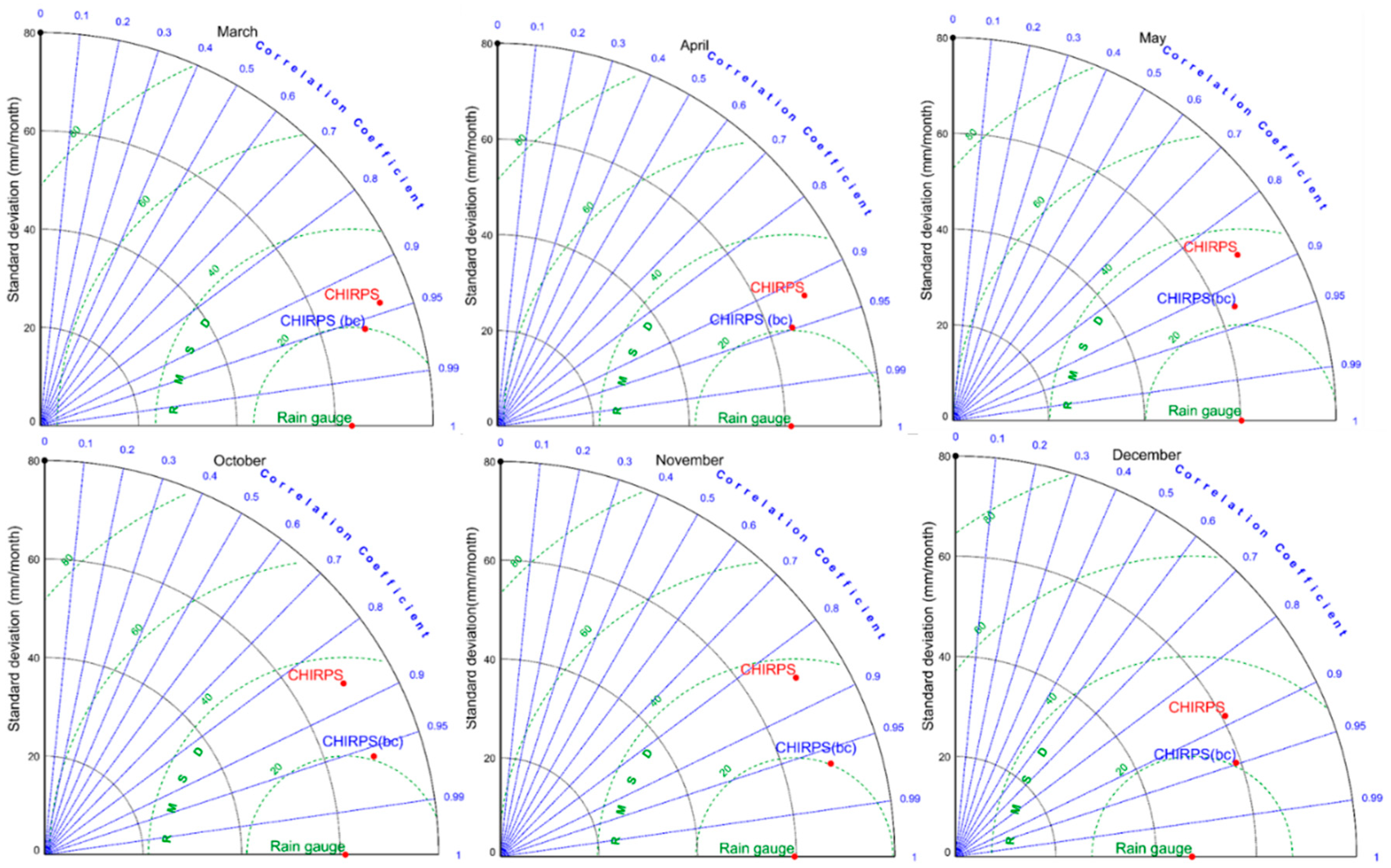
This section describes the monthly assessments of bias correction of CHIRPS rainfall estimates using rain gauge data over East Africa during a validation period of 2003 to 2013. Figure 2 presents the Taylor diagrams displaying the error metrics before (CHIRPS) and after bias corrections (abbreviated with a ‘bc’) during the wet months of March to May, and October to December. These results showed that the Bayesian approach significantly improved the accuracy of the CHIRPS estimates as indicated by the reduced RMSD and increased correlations for all months. The biases showed seasonality and occurred more during OND when compared to the MAM months. During OND, the orographic processes were more dominant and more challenging for the infrared-based satellite rainfall products [13]. The bias increased with an increase in rainfall magnitudes [11] and were largest in April and November. These are the peak rainfall months of the MAM and OND seasons, respectively. These observations of bias dependence on rainfall amounts concurred with [10] over other parts of Africa.
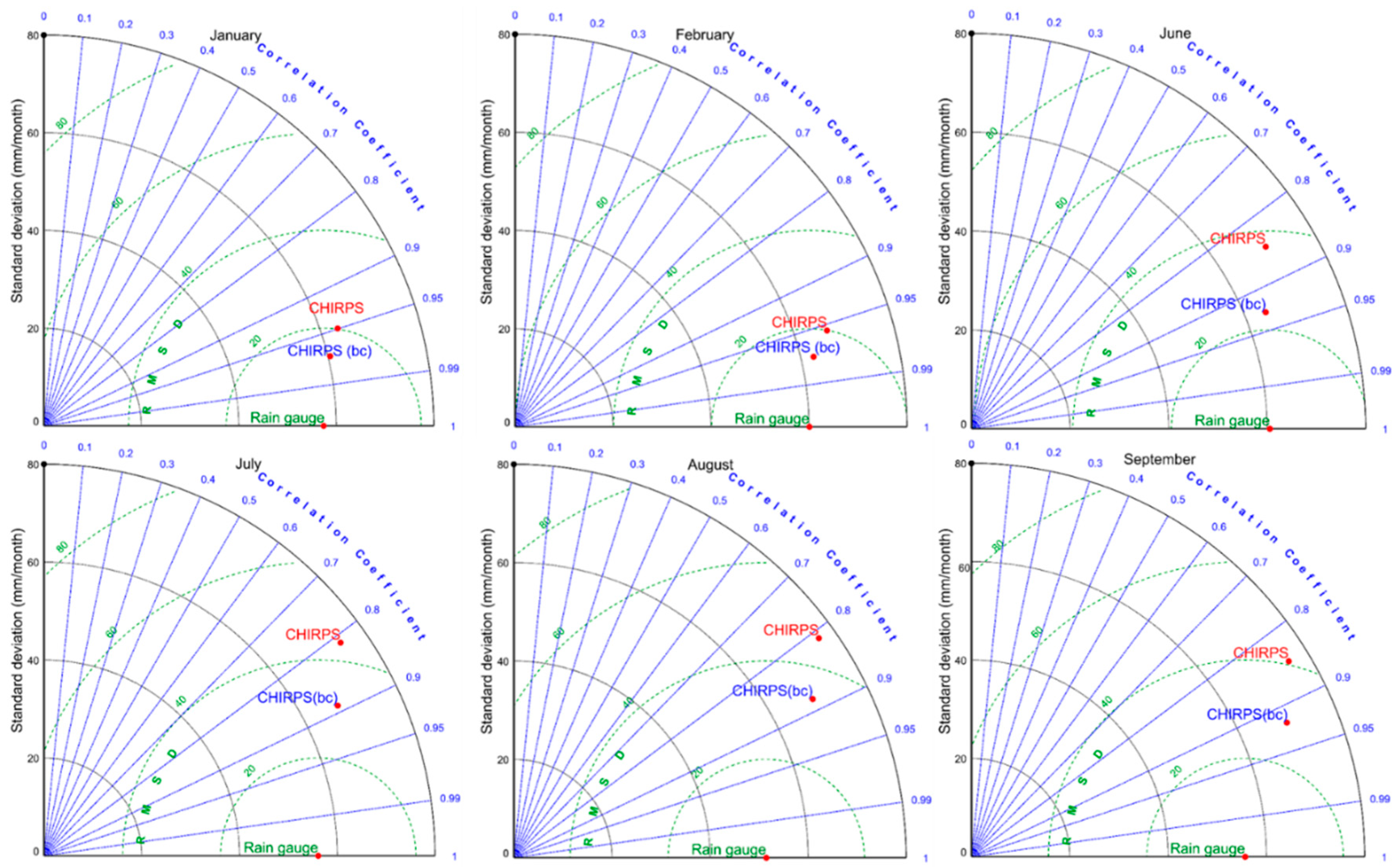
Figure 3 presents the results of the relatively dry months of January, February, and June through September and showed a significant reduction of biases. It was evident that there were increased error magnitudes than during the wet months, mainly from June–September. These errors are attributable to orographic processes during the northeast (January through February) and southeast (June through September) monsoon period. The high grounds inhabit moisture influx inland, thereby limiting the rainfall occurrence to the high ground areas. In their study [33,34], associated Turkana Jets that run parallel to the highlands cause rainfall variabilities during the south-east monsoon season.
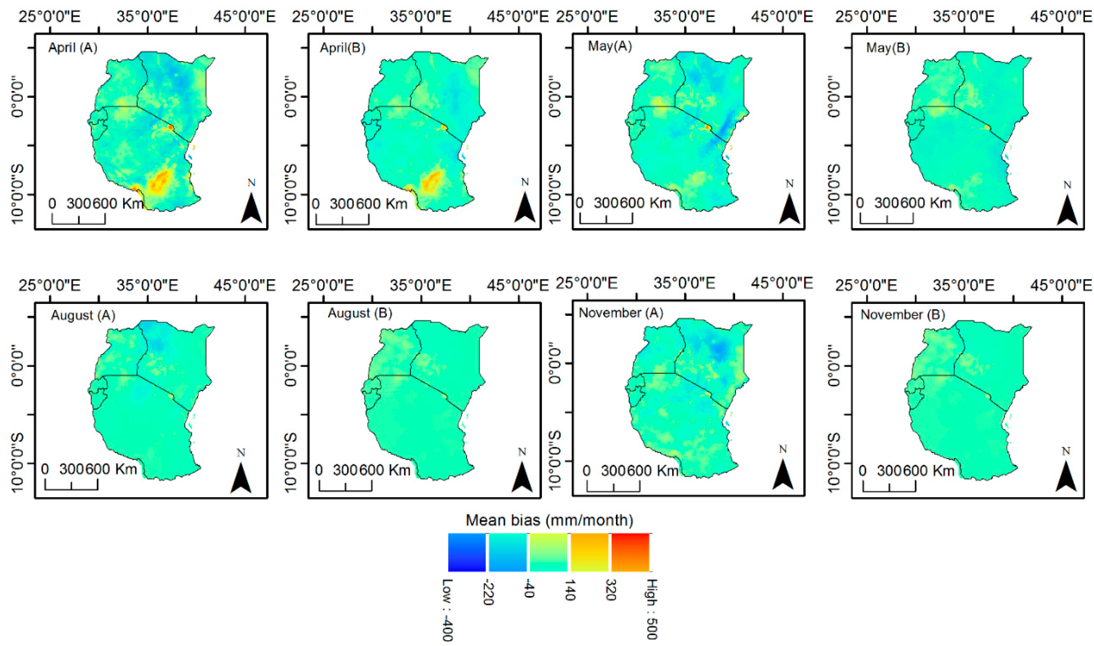
Figure 4 shows the mean bias (2003–2013) derived from CHIRPS and the bias-corrected CHIRPS (bc) relative to rain gauge data for April and May, August, and November. The three wet seasons are representative of March–May, June–August, and October–December, respectively. The spatial patterns display areas of underestimations and overestimations and indicate the areas of improvement after Bayesian applications. It is evident that increased bias followed areas of the highest rainfall amounts. Consequently, the largest underestimations (negative bias) were observed in highly elevated regions of Mt. Kenya in November, around Mt. Elgon in August, and over the coastal areas bordering the Indian Ocean in May. This confirmed that the CHIRPS monthly estimates underestimated high rainfall amounts [29]. These findings were also in line with [11], where observed systematic errors increased with increased rainfall amounts. Evidently, in April, which is the peak rainfall month of MAM, the mean biases were well distributed and attributable to mixed rainfall regime characteristics. Additionally, overestimations (positive bias) were evident in areas around Lake Victoria, eastern parts of Kenya, and Southern Tanzania in April and May. The overestimations arose from cirrus effects common to infrared based products using a cold cloud temperature threshold as they consider the cold cirrus clouds that occur in deep convections as precipitating [11]. It was evident that the approach adequately reduced overestimations except over Southern Tanzania, which showed sparse rain gauge stations (Figure 1) and may therefore not have well-represented rainfall variability. Similarly, a study by [17] used the probability distribution to adjust satellite rainfall estimates and associated overcorrections for the misrepresentation of rainfall variability in sparse rain gauge areas. It is recommended that this approach is sensitive to the inconsistencies of the reference data and does not necessarily modify the satellite rainfall estimates.
Table 1 shows a summary of the monthly error statistics for all months before and after bias corrections and the change of errors in percentages. It was evident the bias-corrected CHIRPS (bc) estimates showed reductions in RMSD and MAE errors and an increase in correlations. One notable observation was the low percentage change in correlations during the relatively dry months. Further observations showed that these months corresponded with the southeast and northeast monsoon months of June through September and December–February, respectively. Therefore, it was evident that the systematic errors locally induced by topographic effects were also externally influenced by the largescale circulations. The low linearity arose from abrupt rainfall variability, hence increasing the average error inconsistencies in time assumed in the Bayesian approach. The overall monthly reduction of RMSD was between 4% and 60%, and the MAE was between 1% and 63%, while the correlations increased up to 21%.
4.1.2. Yearly Evaluations
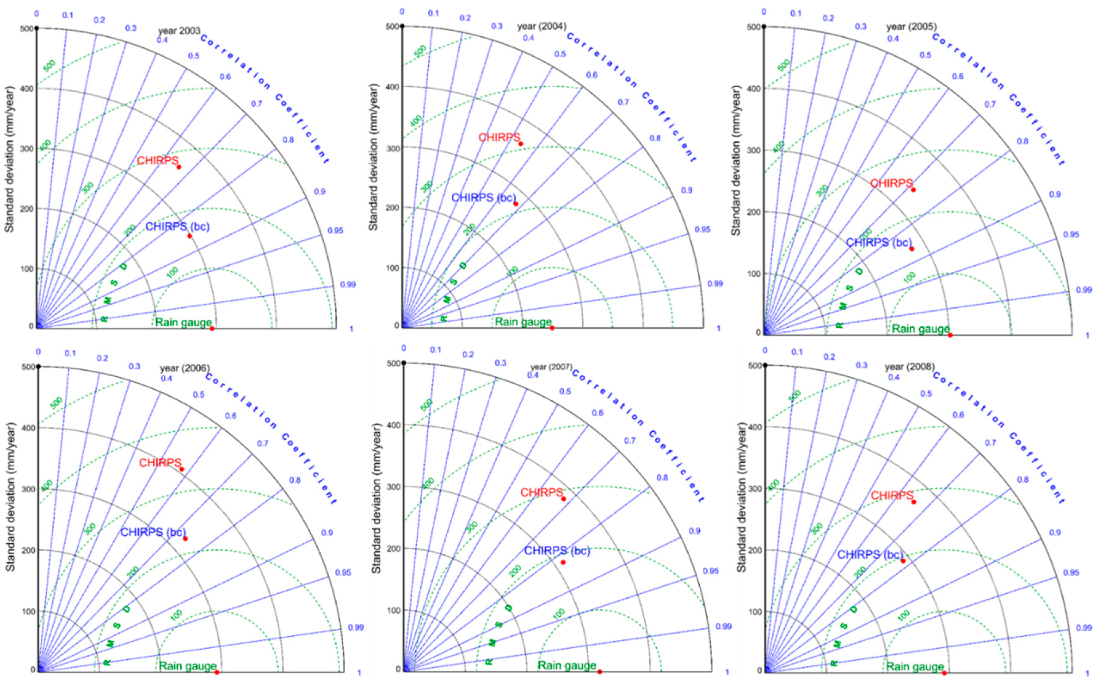
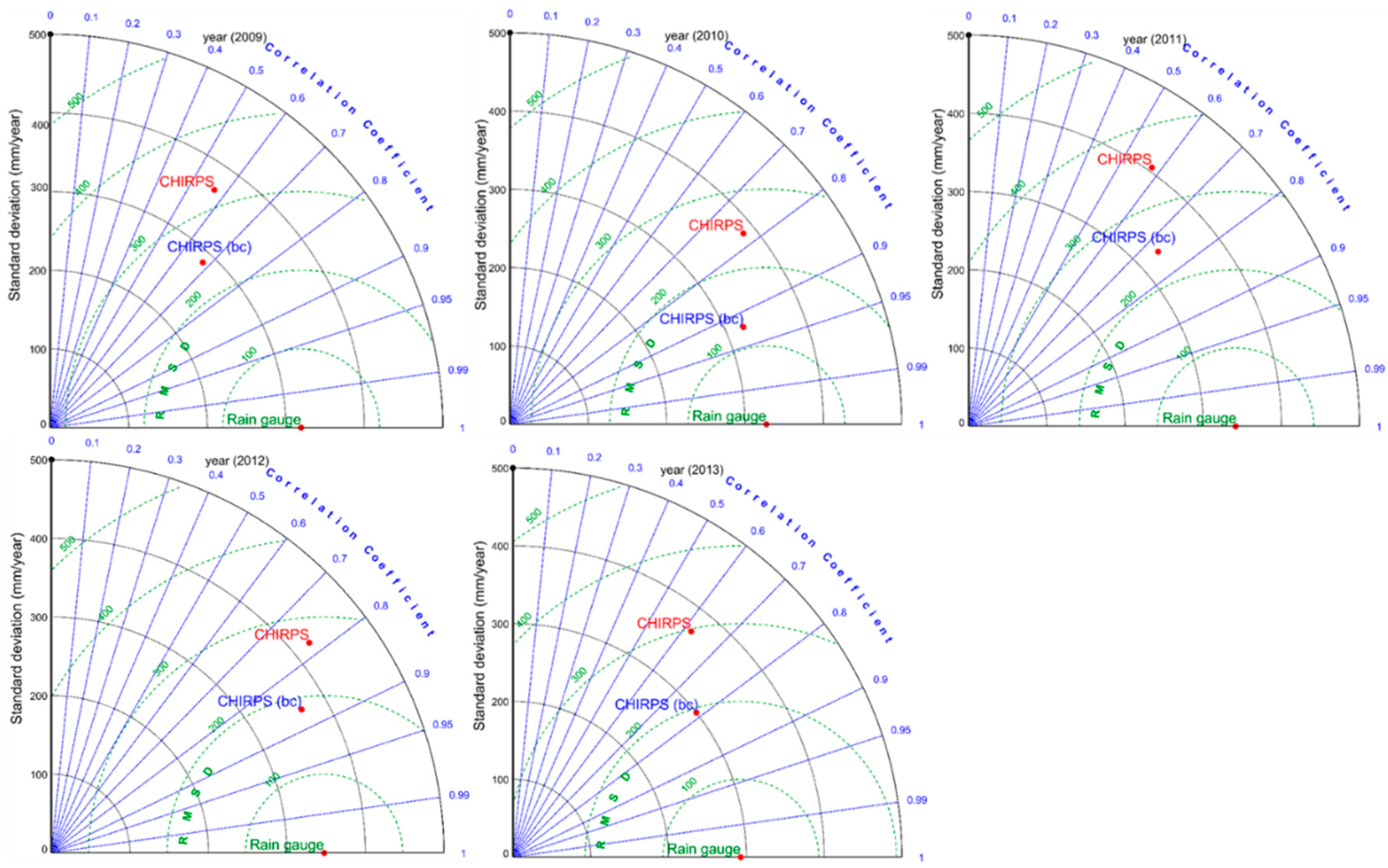
This section describes the annual spatial evaluation of the CHIRPS and bias-corrected CHIRPS (bc) rainfall estimates relating to the rain gauge data during the validation years (2003–2013). Figure 5 and Figure 6 show the Taylor diagrams displaying the error metrics of the RMSD and correlations and their respective standard deviations. It was evident that in all of the years, the CHIRPS rainfall estimates were adjusted towards the rain gauge data as indicated by the reduced RMSD and increased correlation coefficients. Large differences occurred in the years associated with El Niño (2003 and 2006) and the least during the relatively drier year (2005). Therefore, it was clear that systematic errors accumulated with increased rainfall, especially during anomalous years and it is worth noting that the seasonality over East Africa corresponded with the observed bias. This shows the importance of a long-term correction period that is inclusive of the known external variabilities. A notable observation of increased bias was in the year following El Niño, for example, the years 2004, 2007, and 2010. El Niño occurred towards the end of the year in October through December and increased rainfall in the months following may have arisen from recycled water.
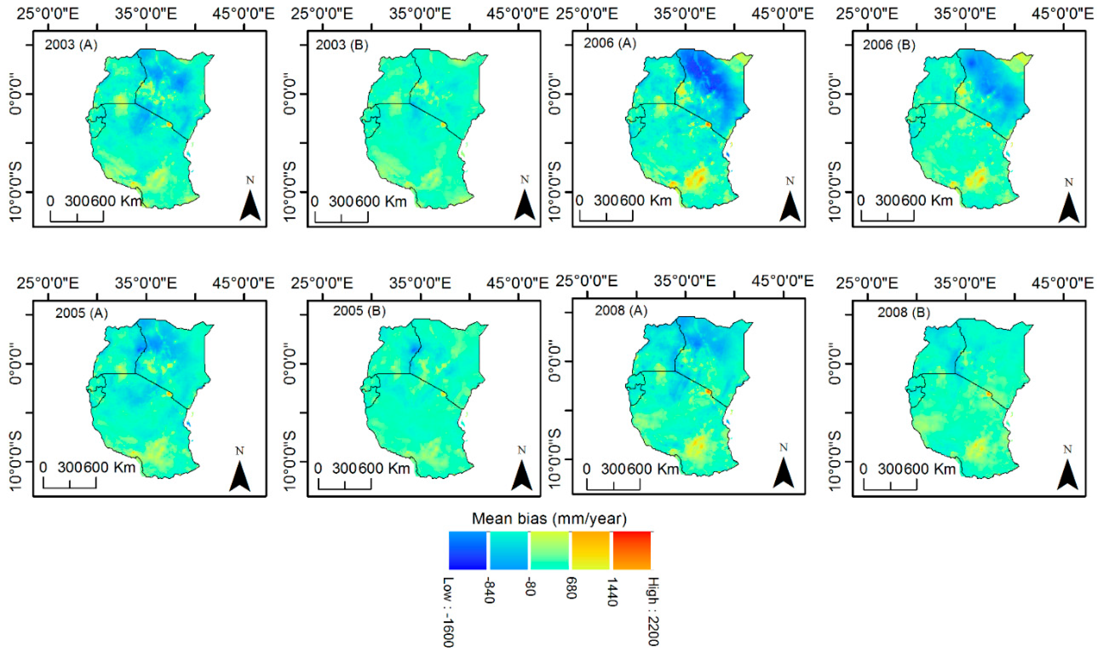
Figure 7 shows the spatial mean bias distribution during the anomalous wet years of 2003 and 2006, the relatively dry (2005), and standard (2008) years. Similar to the monthly analysis, underestimations were evident before bias correction. The Bayesian approach substantially reduced the biases over the high elevated areas of Mt. Kenya in 2006, which was also an El Niño year. Similarly, overestimations were evident around Lake Victoria, Southern Tanzania, near Mt. Elgon, and North-eastern Kenya. Large uncorrected overestimations were observed, particularly in the southern parts of Tanzania and around Mt. Kilimanjaro, which are areas of poor rain gauge network (Figure 1).
Table 2 shows a summary of the yearly error statistics before and after bias corrections, and the change of errors in percentages. There was a remarkable decrease in the RMSD and MAE as well as an increase in correlations after bias corrections. Similar to the monthly analysis, the errors corrected showed a dependence on rainfall magnitude, but also on rainfall regime. As such, the years 2003, and 2009, which were also El Niño years, did not correspond to the highest mean rainfall as El Niño occurred during the short rainfall period of OND. However, the years after (2004 and 2010), had higher rainfall that spread to the MAM rainfall season. Similarly, in 2007 and 2010, the years following El Niño, there was increased rainfall and a correspondingly high percentage of errors corrected. It is worth noting that during the relatively dry year (2005), the percentage of RMSD and MAE corrected was high (46%). This can be attributable to the fact that CHIRPS estimates are designed for drought monitoring, hence there are more consistent mean errors during dry years. In [11], it was observed that the systematic errors were seasonal, hence the importance of understanding the rainfall distribution during the year in a given area.
4.2. Analysis of Bayesian Performance
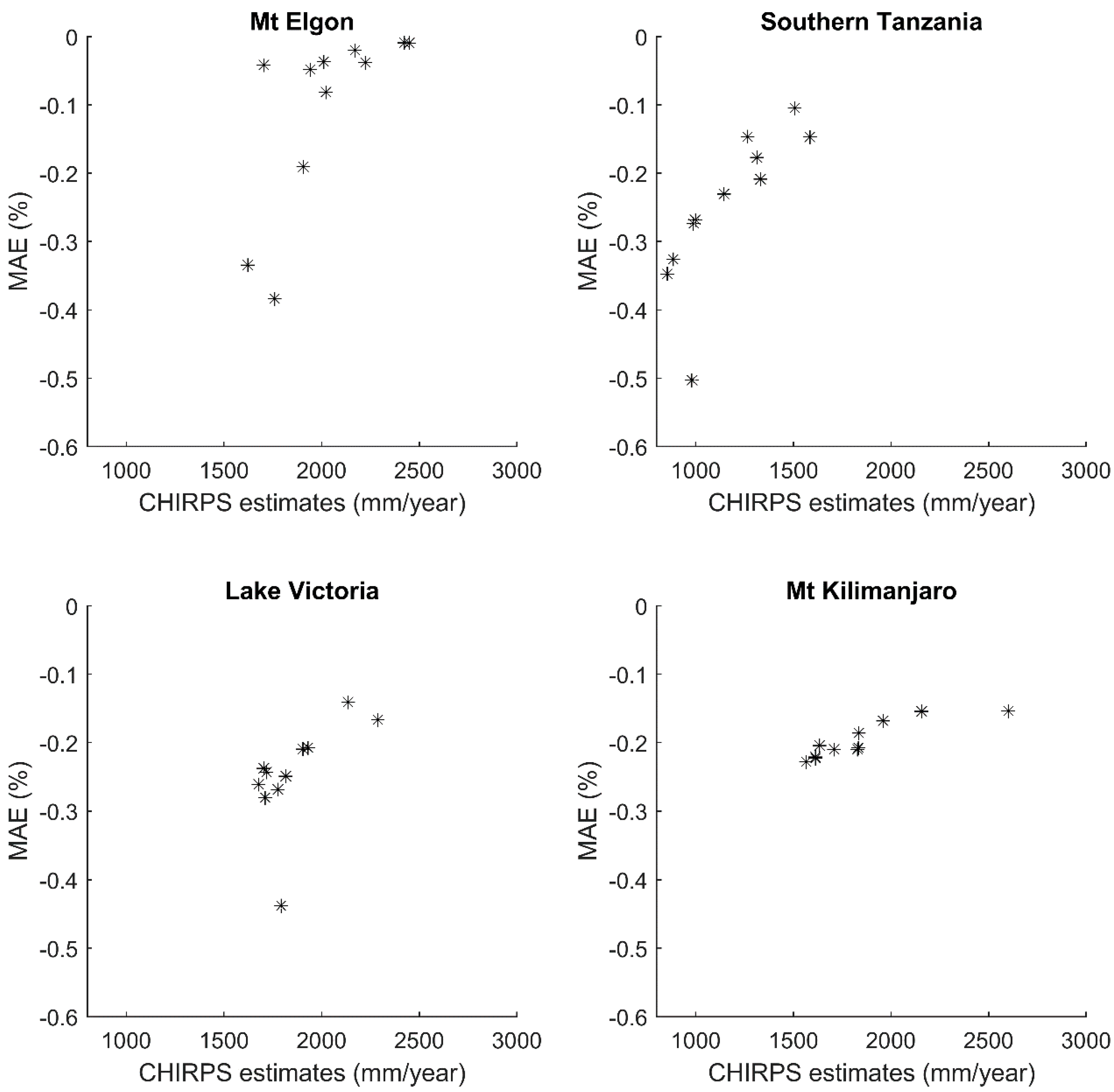
In addition, pixels within the areas of lowest Bayesian performance were assessed using the yearly CHIRPS and bias-corrected (bc) rainfall estimates relative to rain gauge data. Nine pixels from Mt. Elgon, Southern Tanzania, Lake Victoria, and Mt. Kilimanjaro were considered (Figure 1). Figure 8 shows the scatter plots of the uncorrected CHIRPS rainfall estimates and MAE change in percentage after correction. A linear relationship was evident, indicating that as the CHIRPS rainfall estimates increased, the effectiveness of the approach reduced. Further results also showed that for the 11 years of analysis, overestimations were dominant except over Mt. Elgon, which showed isolated incidences of underestimation. CHIRPS overestimates in areas of high rainfall, and this is likely to be attributable to cirrus effects in those areas of deep convection [13].
Table 3 shows a summary of the yearly statistics for the 11-year validation period on Bayesian performance analysis over Mt. Elgon, Southern Tanzania, Lake Victoria, and Mt. Kilimanjaro. These were the areas of largest uncorrected overestimations. The results showed that over the four regions, the lowest MAE in the uncorrected CHIRPS corresponded to the highest percentage of error corrected. This suggests that the retrieval capability of CHIRPS determines the magnitude of errors corrected due to the average error consistencies. Consequently, the MAE errors corresponded to rainfall magnitude, suggesting overestimations increase in years of high rainfall. As such, the relatively dry year of 2005 had substantial MAE errors corrected. Furthermore, observations showed that although each region received different amounts of rainfall in different years, the percentage change in the MAE showed a similar pattern. An example was in the year 2009 over the Mt. Elgon and Lake Victoria areas, where the lowest MAE in CHIRPS rainfall were 49.4 mm/year and 273.5 mm/year, respectively. Consequently, the corrected MAE were the highest (38% and 44%). Similarly, over Southern Tanzania, in 2007, the lowest MAE in CHIRPS was 175.6 mm/year, and corresponded to the highest percentage (50%) of corrected errors. In Mt. Kilimanjaro in 2005, the lowest MAE error in CHIRPS was 1140.4 mm/year and also coincided with the highest percentage error corrected of 23%. These errors of overestimations were attributable to the cold cirrus effect, which infrared based algorithms including CHIRPS consider as precipitating. The Bayesian approach showed little skill in eradicating these errors, partly due to the low misrepresentation of rainfall variability in areas of poor rain gauge distribution in these areas. As such, the rain gauge data were inconsistent in time.
5. Discussion
This study assessed the Bayesian bias correction on CHIRPS v2 using the regionally gridded rain gauge data provided by the ICPAC over East Africa. Although CHIRPS includes some of the rain gauge data used in this study, they were a small percentage derived mainly from the GTS. The ICPAC gridded dataset incorporates all of the available quality controlled meteorological and hydrological rain gauge data from East African member states. Furthermore, a recent study by [13] on the commonly used satellite products including CHIRPS over the region, showed large discrepancies with ground data, especially in high elevated areas. This study aimed to reduce these errors mainly caused by local effects by using Bayesian methods. The correction was on a monthly scale, which is relevant for long-term applications of 33 years (1981–2013). The usage of the approach assumes the mean errors of the input data are consistent in time. The results from the monthly analysis showed that the approach significantly reduced the systematic errors in all months from January to December with varying magnitudes. The corrected biases were mainly of underestimations affecting the high elevated areas attributable to orographic processes. Overestimations affected the areas around Lake Victoria and low-lying areas to the eastern parts of East Africa and Southern Tanzania. This is attributable to the cirrus effects caused by the assignment by infrared sensors in satellite products of all cold clouds as precipitating. It is suggested the cirrus effect affects areas of poor rain gauge networks areas as they misrepresent rainfall variability. As such, the rain gauge data were inconsistent with time, which is an assumption in this approach, hence the low effectiveness of bias correction over those areas. This observation concurred with that in [35] where at monthly time scales, CHIRPS overestimated low rainfall amounts and underestimated high rainfall amounts. However, the underestimations were associated with local processes, while overestimations were more likely to arise from cirrus effects occurring in deep convection [36]. Consequently, cirrus effects are observed mainly in months of increased rainfall in April and May. The study further revealed that during the southeast and northeast monsoon months of June to September and December to February, low linearity improvements were observed as indicated by corrections change. The inhibition of rainfall further inland from the low-level diffluence of the monsoon winds leads to the dominance of orographic processes [13]. Consequently, the rainfall variability in Eastern Kenya and Southern Tanzania coincided with Turkana low-level jets [33,37], which link the local rainfall variabilities to external influences. These abrupt changes lead to increased rainfall variabilities, hence the reduced linearity assumed in the Bayesian approach.
The yearly analysis showed an increase of the corrected biases attributable to the reduced rainfall variability. Similar to monthly assessments, the underestimations in corrected data were more dominant over the high elevated areas. Similarly, overestimations were observed in areas around Lake Victoria, Mt. Elgon, Eastern Kenya, and Southern Tanzania. These are areas of poor rain gauge distribution, and the misrepresentation of rainfall variabilities led to a reduction in the minimal errors. Consequently, the CHIRPS rainfall estimates approached its uncorrected state. One advantage of the method the incorporation of the error variance in the correction, and the correction only applies when the reference dataset is reliable, and errors are systematic, not random. Although 2006, which was also an El Niño, received the highest rainfall, the percentage of errors corrected was not equivalently high. This suggests that the errors are not only dependent on rainfall magnitude, but on distribution in time. El Niño years occur during the October–December rainfall months, which also have fewer rain days when compared to the March–May rainfall months [38]. Consequently, the years following the El Niño years were observed to have high rainfall and a large percentage of bias were also corrected. This high rainfall after El Niño is suggested to arise during the MAM rainfall months. However, it is worth noting that East Africa has high rainfall variability and the yearly analysis presented here is for the whole region. This observation is essential as the systematic errors occur more with increased rainfall amounts, and also depend on the distribution of rainfall in time and space.
Further annual assessments of the performance of Bayesian approach were conducted on selected pixels centered in areas of large CHIRPS overestimations. Nine pixels from each region over Mt. Elgon, Southern Tanzania, Lake Victoria, and Mt. Kilimanjaro were selected. MAE in percentage change of CHIRPS and bias-corrected CHIRPS relative to rain gauge data were used to quantify the relationships. Results showed that CHIRPS overestimated in all years (2003–2013) over those areas except for a few incidences of underestimation over Mt. Elgon. Furthermore, the MAE percentage change showed a linear relationship with rainfall magnitudes. An increase in rainfall magnitude corresponded with a decrease in the percentage of MAE change. This showed that there were uncorrected errors during high rainfall periods. It is understandable that cirrus coexists in deep convective systems [36] that are also related to high rainfall amounts. Overestimations in the cirrus effect have also been observed in infrared based products in Eastern Africa [37]. The years 2005, 2007, and 2009 showed the lowest annual rainfall in these regions, and consequently, the highest MAE percentage change. The designation of CHIRPS is for dry conditions; hence the mean errors are consistent in time, hence an increased Bayesian performance. Similar findings in a recent study [38] showed that CHIRPS had low rainfall detection during the wet season. The Bayesian approach showed low skill in reducing errors attributed to cirrus effects in areas of poor rain gauge network due to the misrepresentation of rainfall variability.
6. Conclusions
Rain gauge distributions are on the decline, and satellite rainfall estimates are increasingly used to complement the sparse network. However, rain gauges continue to be used as reference data to validate the incoming satellite products as they offer the most direct information on local rainfall variabilities. This is understandable in developing countries where other ground observations like weather radar are too expensive. However, considering the decreasing trend in rain gauge density, other measures like gridding the available gauge data are preferred. As such, validation exercises are enhanced, which may otherwise become increasingly compromised in the future. This impact may be much more severe for long-term data applications. This study assessed the applicability of the Bayesian approach with an existing historical rain gauge dataset to create consistent satellite rainfall data for long-term applications. The gridded rain gauge dataset was developed by ICPAC to safeguard the decreasing rain gauge information over East Africa.
CHIRPS was chosen based on its close correspondence with rain gauge datasets when compared to other commonly used products over the region [13]. However, CHIRPS, like other satellite-derived products, exhibit systematic errors that vary from place to place. In mountainous areas like East Africa, the retrieval of topographic processes is challenging. These biases need to be reduced to increase the effectiveness of this product over the region. It is understandable that high elevated areas play a significant role in water availability and minimizing these errors would improve the representative of the CHIRPS estimates. Furthermore, as CHIRPS has a high (0.05°) spatial scale, it can be used for future reference for the incoming coarser satellite products. The study aimed at temporally and spatially evaluating how CHIRPS rainfall estimates compared with the gridded rain gauge data in magnitude and distributions after bias correction. For the Bayesian correction, a historical dataset of 22 years of data was used as the calibration dataset, and the ensuing 11 years were used for the validation.
Monthly analysis showed that CHIRPS estimates had systematic errors mainly of underestimations arising in high elevated areas and their surroundings. The approach adequately reduced them in both wet and relatively dry months. The study revealed large biases emerged during the wet months and less so for the relatively drier months. This is understandable as the CHIRPS algorithm has been optimized for drought monitoring, that is, for better accuracy during drier periods. As such, in April, which is the peak rainfall month of the March to May rainfall season, the biases were distributed over East Africa. In May, they were observed near the Lake Victoria region and coastal areas of Kenya where high rainfall is experienced during this month. During the south-east monsoon month of August, they were situated on the border between Kenya and Uganda following the highest rainfall amounts in the June through August rainfall season. However, low linearity improvements of the negative biases were observed during the southeast and northeast monsoon months in June to September and December to February, respectively. These were attributable to indirect rainfall variability related to external factors in high elevated areas. The study revealed that these monsoons influenced orographic processes, reducing further inland impacts. Furthermore, the Bayesian approach assumes linear relationships between rainfall variability and the mean errors. Overestimations were dominant over Lake Victoria, Southern Tanzania, Mt. Elgon, Eastern Kenya, and the Kilimanjaro region. These biases were attributable to cirrus effects, which in IR based products (like CHIRPS) often results in an overestimation of precipitation. Adequate bias reduction was observed except in a few areas over Southern Tanzania and part of Lake Victoria where misrepresentation due to the sparse rain gauge network affected the correction. It is worth noting that inconsistencies of average errors, due to sparse rain gauge distributions were attributable to CHIRPS large uncorrected errors in those areas. A remarkable difference in the approach to other methods is its ability to leave the satellite estimates close to the uncorrected state when the reference data is inconsistent in time. The overall monthly average reduction indicates that the RMSD reduced between 4% and 60%, and the MAE between 1% and 63%, while the correlations improved by up to 21%, as shown in Table 1.
The yearly analysis showed an increase in the corrected biases which is associated to the reduced rainfall variability at this scale. Similar to monthly findings, the corrected underestimations were more dominant on high elevated areas and were in areas of high rainfall magnitudes that showed seasonality. The study observed that the corrected biases were more during years of high rainfall magnitude. Although large biases were evident during El Niño year of 2006 which also has highest rainfall amount, not all El Niño years showed similar results. This is understandable as El Niño years occur during the October–December rainfall months, but its effect spreads to the March–May rainfall months. As a result, the year that followed was observed to have high rainfall, hence an increased in the biases corrected. An example is shown in the 2003, 2006, and 2009 El Niño years whereby an increased rainfall average amount was observed a year after in 2004, 2007, and 2010. Consequently, a higher percentage of bias were corrected. This observation is vital as the systematic errors are increased with increased rainfall amounts, but are also dependent on the distribution of the rainfall in time. The overall yearly average reduction indicated that the RMSD was reduced by between 17% and 49%, and the MAE was reduced by between 13% and 48%, while the correlations increased by between 9% and 17%, as shown in Table 2.
Further assessments of the performance of the Bayesian approach were carried out using selected pixels (Figure 1) in areas of substantial uncorrected bias. These areas included Mt. Elgon, Southern Tanzania, Lake Victoria, and the Mt. Kilimanjaro areas. Nine pixels from the areas with the largest overestimations were used for the extraction of average rainfall for CHIRPS, and bias-corrected CHIRPS (bc) and compared with the corresponding rain gauge dataset. The percentage change in MAE quantified their relationships. This analysis indicated that CHIRPS considerably overestimated rainfall in those areas of sparse rain gauge distributions. The highest corrected MAE were observed in the years of the lowest MAE. Observations showed that the years 2005, 2007, and 2009 had the lowest annual rainfall in these regions, and consequently, the highest MAE decrease. Although each region received different amounts of rain over the validation period, the errors in corrected estimates showed a similar trend. The lowest MAE before correction corresponded with the highest percentage of corrected errors spatially and temporally. This can be understood as shallow convections in cirrus effects are minimal. Conversely, in the years and areas of deep convections, cirrus clouds increase. However, in areas of relatively dense rain gauges, cirrus related errors are minimized. For example, in the year 2009 over the Mt. Elgon and Lake Victoria areas, the lowest MAEs observed before correction were 49.5 mm/year and 273.5 mm/year, respectively. Consequently, those were the areas of highest corrected MAE, at 38% and 44%, respectively. Similarly, over Southern Tanzania, in the year 2007, the lowest MAE was 175.6 mm/year, and was consistent with the highest corrected MAE of 50%. In Mt. Kilimanjaro, in 2005, the lowest MAE error was 1140.6 mm/year and coincided with the highest percentage improvement of 23%. Therefore, overcorrections were adequately addressed spatially and temporally when rainfall was low in areas of sparse rain gauges, but remain unaddressed in deep convection attributed to monsoons. This effect was minimal in densely distributed rain gauge areas due to the increased representation of rainfall variability.
The Bayesian approach is recommended to adjust rainfall estimates of other algorithms with long-term historical records that are representative of rainfall variability of the area under consideration. The method is suitable for the reduction of systematic errors, especially in high elevated regions. It is, however, sensitive to sparse rain gauge distributions in regions of deep convective systems due to cirrus effects that cause overestimations. Therefore, with a good quality rain gauge network, the approach works better in those areas. It is recommended to have the reference data of a higher or equal spatial scale for higher rainfall spatial representation.
Author Contributions
All three authors contributed in concept building and manuscript preparation. M.W.K. analyzed the data and drafted the manuscript. Z.S. and J.C.B.H. provided conceptual advice and contributed to the overall writing and approval of the final manuscript.
Acknowledgments
This work was made possible through the funding provided by the Netherlands Fellowship Programs (NFP), and we greatly appreciate their support. The University provided funds for open access.
Conflicts of Interest
The authors declare no conflict of interest.
References
- Kidd, C.; Bauer, P.; Turk, J.; Huffman, G.J.; Joyce, R.; Hsu, K.L.; Braithwaite, D. Intercomparison of high-resolution precipitation products over northwest Europe. J. Hydrometeorol. 2012, 13, 67–83. [Google Scholar] [CrossRef]
- Villarini, G.; Krajewski, W.F. Empirically-based modeling of spatial sampling uncertainties associated with rainfall measurements by rain gauges. Adv. Water Resour. 2008, 31, 1015–1023. [Google Scholar] [CrossRef]
- Dibike, Y.B.; Coulibaly, P. Validation of hydrological models for climate scenario simulation: The case of Saguenay watershed in Quebec. Hydrol. Process. 2007, 21, 3123–3135. [Google Scholar] [CrossRef]
- Sorooshian, S.; Hsu, K.L.; Gao, X.; Gupta, H.V.; Imam, B.; Braithwaite, D. Evaluation of persiann system satellite-based estimates of tropical rainfall. Bull. Am. Meteorol. Soc. 2000, 81, 2035–2046. [Google Scholar] [CrossRef]
- Feidas, H.; Lagouvardos, K.; Kotroni, V.; Cartalis, C. Application of three satellite techniques in support of precipitation forecasts of a NWP model. Int. J. Remote Sens. 2005, 26, 5393–5417. [Google Scholar] [CrossRef]
- Krajewski, W.F.; Ciach, G.J.; McCollum, J.R.; Bacotiu, C. Initial validation of the global precipitation climatology project monthly rainfall over the United States. J. Appl. Meteorol. 2000, 39, 1071–1086. [Google Scholar] [CrossRef]
- Adler, R.F.; Huffman, G.J.; Chang, A.; Ferraro, R.; Xie, P.; Janowiak, J.; Arkin, P. The version 2 global precipitation climatology project (GPCP) monthly precipitation analysis. J. Hydrometeorol. 2003, 4, 1147–1167. [Google Scholar] [CrossRef]
- Arkin, P.A.; Xie, P.P. The global precipitation climatology project—1st algorithm intercomparison project. Bull. Am. Meteorol. Soc. 1994, 75, 401–419. [Google Scholar] [CrossRef]
- Maidment, R.I.; Grimes, D.I.F.; Allan, R.P.; Greatrex, H.; Rojas, O.; Leo, O. Evaluation of satellite-based and model re-analysis rainfall estimates for Uganda. Meteorol. Appl. 2013, 20, 308–317. [Google Scholar] [CrossRef]
- Tote, C.; Patricio, D.; Boogaard, H.; van der Wijngaart, R.; Tarnavsky, E.; Funk, C. Evaluation of satellite rainfall estimates for drought and flood monitoring in Mozambique. Remote Sens. 2015, 7, 1758–1776. [Google Scholar] [CrossRef]
- AghaKouchak, A.; Mehran, A.; Norouzi, H.; Behrangi, A. Systematic and random error components in satellite precipitation data sets. Geophys. Res. Lett. 2012, 39. [Google Scholar] [CrossRef] [Green Version]
- Abera, W.; Brocca, L.; Rigon, R. Comparative evaluation of different satellite rainfall estimation products and bias correction in the Upper Blue Nile (UBN) basin. Atmos. Res. 2016, 178, 471–483. [Google Scholar] [CrossRef]
- Kimani, M.W.; Hoedjes, J.C.B.; Su, Z.B. An assessment of satellite-derived rainfall products relative to ground observations over East Africa. Remote Sens. 2017, 9, 430. [Google Scholar] [CrossRef]
- Maurer, E.P.; Pierce, D.W. Bias correction can modify climate model simulated precipitation changes without adverse effect on the ensemble mean. Hydrol. Earth Syst. Sci. 2014, 18, 915–925. [Google Scholar] [CrossRef] [Green Version]
- Mateus, P.; Borma, L.S.; da Silva, R.D.; Nico, G.; Catalao, J. Assessment of two techniques to merge ground-based and trmm rainfall measurements: A case study about Brazilian Amazon rainforest. GISci. Remote Sens. 2016, 53, 689–706. [Google Scholar] [CrossRef]
- Vila, D.A.; de Goncalves, L.G.G.; Toll, D.L.; Rozante, J.R. Statistical evaluation of combined daily gauge observations and rainfall satellite estimates over continental South America. J. Hydrometeorol. 2009, 10, 533–543. [Google Scholar] [CrossRef]
- Tian, Y.D.; Peters-Lidard, C.D.; Eylander, J.B. Real-time bias reduction for satellite-based precipitation estimates. J. Hydrometeorol. 2010, 11, 1275–1285. [Google Scholar] [CrossRef]
- Stokstad, E. Hydrology—Scarcity of rain, stream gages threatens forecasts. Science 1999, 285, 1199–1200. [Google Scholar] [CrossRef]
- Dinku, T.; Ceccato, P.; Grover-Kopec, E.; Lemma, M.; Connor, S.J.; Ropelewski, C.F. Validation of satellite rainfall products over East Africa’s complex topography. Int. J. Remote Sens. 2007, 28, 1503–1526. [Google Scholar] [CrossRef]
- Talagrand, O. Assimilation of observations, an introduction (gtspecial issueltdata assimilation in meteology and oceanography: Theory and practice). J. Meteorol. Soc. Jpn. Ser. II 1997, 75, 191–209. [Google Scholar] [CrossRef]
- Seiz, G.; Foppa, N. National climate observing system of switzerland (GCOS Switzerland). Adv. Sci. Res. 2011, 6, 95–102. [Google Scholar] [CrossRef]
- Funk, C.C.; Peterson, P.J.; Landsfeld, M.F.; Pedreros, D.H.; Verdin, J.P.; Rowland, J.D.; Romero, B.E.; Husak, G.J.; Michaelsen, J.C.; Verdin, A.P. A Quasi-Global Precipitation Time Series for Drought Monitoring; U.S. Geological Survey Data Series: Reston, VA 20192, USA, 2014. [Google Scholar]
- IGAD. Available online: http://www.Icpac.Net/ (accessed on 6 November 2015).
- Funk, C.; Nicholson, S.E.; Landsfeld, M.; Klotter, D.; Peterson, P.; Harrison, L. The centennial trends greater horn of Africa precipitation dataset. Sci. Data 2015, 2, 150050. [Google Scholar] [CrossRef] [PubMed]
- ICPAC. Available online: http://chg-wiki.geog.ucsb.edu/wiki/GeoCLIM (accessed on 6 November 2015).
- SRTM 90m Digital Elevation Database v4.1. Available online: http://www.Cgiar-csi.Org/data/srtm-90m-digital-elevation-database-v4-1 (accessed on 5 July 2018).
- Carlin, B.P.; Louis, T.A. Bayes and Empirical Bayes Methods for Data Analysis; Chapman and Hall: London, UK, 1996; p. 399. [Google Scholar]
- Suwendi, A.; Allebach, J.P. Nearest-neighbor and bilinear resampling factor estimation to detect blockiness or blurriness of an image. J. Electron. Imaging 2008, 17, 023005. [Google Scholar]
- Tan, M.L.; Ficklin, D.L.; Dixon, B.; Ibrahim, A.L.; Yusop, Z.; Chaplot, V. Impacts of DEM resolution, source, and resampling technique on SWAT-simulated streamflow. Appl. Geogr. 2015, 63, 357–368. [Google Scholar] [CrossRef] [Green Version]
- Taylor, K.E. Summarizing multiple aspects of model performance in a single diagram. J. Geophys. Res. Atmos. 2001, 106, 7183–7192. [Google Scholar] [CrossRef] [Green Version]
- Nicholson, S. The turkana low-level jet: Mean climatology and association with regional aridity. Int. J. Climatol. 2016, 36, 2598–2614. [Google Scholar] [CrossRef]
- Kinuthia, J.H.; Asnani, G.C. A newly found jet in North Kenya (Turkana Channel). Mon. Weather Rev. 1982, 110, 1722–1728. [Google Scholar] [CrossRef]
- Trejo, F.J.P.; Barbosa, H.A.; Penaloza-Murillo, M.A.; Moreno, M.A.; Farias, A. Intercomparison of improved satellite rainfall estimation with chirps gridded product and rain gauge data over Venezuela. Atmosfera 2016, 29, 323–342. [Google Scholar] [CrossRef]
- Sassen, K.; Wang, Z.; Liu, D. Cirrus clouds and deep convection in the tropics: Insights from CALIPSO and CloudSat. J. Geophys. Res. Atmos. 2009, 114. [Google Scholar] [CrossRef] [Green Version]
- Kinuthia, J.H. Horizontal and vertical structure of the lake Turkana jet. J. Appl. Meteorol. 1992, 31, 1248–1274. [Google Scholar] [CrossRef]
- Indeje, M.; Semazzi, F.H.M.; Ogallo, L.J. Enso signals in East African rainfall seasons. Int. J. Climatol. 2000, 20, 19–46. [Google Scholar] [CrossRef]
- Young, M.P.; Williams, C.J.R.; Chiu, J.C.; Maidment, R.I.; Chen, S.H. Investigation of discrepancies in satellite rainfall estimates over Ethiopia. J. Hydrometeorol. 2014, 15, 2347–2369. [Google Scholar] [CrossRef]
- Paredes-Trejo, F.J.; Barbosa, H.A.; Kumar, T.V.L. Validating chirps-based satellite precipitation estimates in northeast Brazil. J. Arid Environ. 2017, 139, 26–40. [Google Scholar] [CrossRef]
Figure 1.
Map of East Africa with the Shuttle Radar Topography Mission (SRTM) 90 m digital elevation model. Rain gauge station distributions used for gridding are highlighted in black. In red are the selected pixels for assessments.
Figure 1.
Map of East Africa with the Shuttle Radar Topography Mission (SRTM) 90 m digital elevation model. Rain gauge station distributions used for gridding are highlighted in black. In red are the selected pixels for assessments.

Figure 2.
Monthly Taylor diagrams displaying the statistical comparison between the Climate Hazards Group Infrared Precipitation with Stations (CHIRPS) (red) and bias-corrected CHIRPS (bc) (blue) estimates with corresponding rain gauge data (green) as the reference. Shown are the wet months of the rainfall seasons (March–May and October–December) over a period of 11 years (2003–2013). The azimuthal angle represents the correlation coefficient; radial distance is the standard deviation (mm/month), and green contours represent RMSD (mm/month).

Figure 3.
Same as for Figure 2, but for the relatively drier months of January, February, June–August and September.
Figure 3.
Same as for Figure 2, but for the relatively drier months of January, February, June–August and September.

Figure 4.
Monthly mean bias derived from averages (2003–2013) of rain gauge data and satellite rainfall estimates of CHIRPS (A) and bias corrections (CHIRPS (bc)) (B).
Figure 4.
Monthly mean bias derived from averages (2003–2013) of rain gauge data and satellite rainfall estimates of CHIRPS (A) and bias corrections (CHIRPS (bc)) (B).

Figure 5.
Taylor diagrams displaying the statistical comparison between the CHIRPS (red) and bias-corrected (blue) CHIRPS estimates with corresponding rain gauge data (green) as the reference for years 2003–2008. The azimuthal angle represents the correlation coefficient; the radial distance represents the standard deviation (mm/year), and the green contours represent RMSD (mm/year).

Figure 6.
As per Figure 5, but for the years 2009–2013.
Figure 6.
As per Figure 5, but for the years 2009–2013.

Figure 7.
Yearly spatial bias patterns derived from the averages of the anomalous wet years (2003 and 2006), the dry (2005), and standard (2008) of the CHIRPS and bias-corrected CHIRPS (bc) abbreviated as (A,B), respectively, relative to the rain gauge data.
Figure 7.
Yearly spatial bias patterns derived from the averages of the anomalous wet years (2003 and 2006), the dry (2005), and standard (2008) of the CHIRPS and bias-corrected CHIRPS (bc) abbreviated as (A,B), respectively, relative to the rain gauge data.

Figure 8.
Yearly scatter plots for of pixels in areas of lowest bias correction.


Table 1.
Statistics for the monthly spatial evaluation.
| Months | CC | CC (bc) | Change (%) | RMSD | RMSD (bc) | Change (%) | MAE | MAE (bc) | Change (%) | Rainfall (mm/month) |
|---|---|---|---|---|---|---|---|---|---|---|
| Jan | 0.95 | 0.98 | 2 | 23.1 | 13 | -45 | 17.6 | 9 | -49 | 88.0 |
| Feb | 0.96 | 0.97 | 2 | 23.1 | 15 | -37 | 14.9 | 10 | -31 | 70.3 |
| Mar | 0.87 | 0.90 | 3 | 40.1 | 31 | -22 | 24.7 | 23 | -9 | 105.5 |
| Apr | 0.47 | 0.61 | 14 | 64.3 | 48 | -25 | 43.1 | 28 | -35 | 155.1 |
| May | 0.77 | 0.94 | 17 | 49.5 | 25 | -50 | 36.2 | 20 | -45 | 103.5 |
| Jun | 0.87 | 0.97 | 10 | 22.8 | 10 | -58 | 15.8 | 6 | -61 | 38.4 |
| Jul | 0.89 | 0.98 | 9 | 20.1 | 8 | -60 | 12.0 | 5 | -63 | 31.9 |
| Aug | 0.89 | 0.98 | 9 | 24.1 | 11 | -56 | 14.2 | 6 | -57 | 38.8 |
| Sep | 0.92 | 0.97 | 6 | 19.3 | 13 | -34 | 13.3 | 8 | -43 | 39.4 |
| Oct | 0.95 | 0.95 | 0 | 21.1 | 19 | -11 | 16.9 | 15 | -11 | 87.1 |
| Nov | 0.72 | 0.94 | 21 | 41.4 | 27 | -35 | 29.3 | 23 | -22 | 129.5 |
| Dec | 0.92 | 0.92 | 0 | 27.2 | 26 | -4 | 20.7 | 20 | -1 | 127.0 |
Table 2.
Statistics for the yearly spatial evaluation.
| Years | CC | CC (bc) | Change (%) | RMSD | RMSD (bc) | Change (%) | MAE | MAE (bc) | Change (%) | Rainfall (mm/year) |
|---|---|---|---|---|---|---|---|---|---|---|
| 2003 | 0.71 | 0.88 | 17 | 264 | 145 | −45 | 197 | 107 | −46 | 847 |
| 2004 | 0.54 | 0.68 | 14 | 277 | 183 | −34 | 206 | 131 | −36 | 962 |
| 2005 | 0.72 | 0.86 | 15 | 241 | 138 | −43 | 178 | 96 | −46 | 772 |
| 2006 | 0.58 | 0.74 | 16 | 449 | 324 | −28 | 312 | 225 | −28 | 1234 |
| 2007 | 0.68 | 0.83 | 15 | 276 | 155 | −44 | 199 | 107 | −46 | 951 |
| 2008 | 0.66 | 0.78 | 12 | 270 | 168 | −38 | 201 | 123 | −39 | 917 |
| 2009 | 0.57 | 0.68 | 11 | 256 | 178 | −30 | 195 | 131 | −33 | 887 |
| 2010 | 0.77 | 0.92 | 15 | 261 | 134 | −49 | 187 | 97 | −48 | 943 |
| 2011 | 0.58 | 0.74 | 16 | 348 | 290 | −17 | 258 | 224 | −13 | 911 |
| 2012 | 0.78 | 0.87 | 9 | 258 | 205 | −21 | 191 | 155 | −19 | 866 |
| 2013 | 0.62 | 0.79 | 17 | 316 | 264 | −17 | 239 | 204 | −15 | 847 |
Table 3.
Statistics for the yearly Bayesian performance analysis.
| Mt Elgon | Southern Tanzania | |||||
|---|---|---|---|---|---|---|
| Years | MAE | MAE (bc) | Change (%) | MAE | MAE (bc) | Change (%) |
| 2003 | 105.2 | 85.2 | −19 | 270.9 | 182.6 | −33 |
| 2004 | 167.3 | 160.3 | −4 | 423.0 | 334.7 | −21 |
| 2005 | 56.2 | 37.4 | −33 | 254.3 | 166.0 | −35 |
| 2006 | 771.7 | 764.8 | −1 | 601.4 | 513.0 | −15 |
| 2007 | 143.9 | 137.0 | −5 | 175.6 | 87.3 | −50 |
| 2008 | 113.1 | 103.9 | −8 | 498.3 | 410.0 | −18 |
| 2009 | 49.4 | 30.5 | −38 | 383.2 | 294.8 | −3 |
| 2010 | 182.9 | 176.0 | −4 | 322.6 | 234.3 | −27 |
| 2011 | 347.9 | 341.0 | −2 | 844.4 | 756.1 | −10 |
| 2012 | 728.5 | 721.6 | −1 | 329.6 | 241.3 | −27 |
| 2013 | 188.8 | 181.9 | −4 | 602.8 | 514.5 | −15 |
| Lake Victoria | Mt Kilimanjaro | |||||
| MAE | MAE (bc) | Change (%) | MAE | MAE (bc) | Change (%) | |
| 2003 | 504.6 | 384.8 | −24 | 1167.7 | 907.7 | −22 |
| 2004 | 492.6 | 372.8 | −24 | 1254.7 | 994.7 | −21 |
| 2005 | 459.2 | 339.4 | −26 | 1140.4 | 880.5 | −23 |
| 2006 | 720.4 | 600.5 | −17 | 1692.8 | 1432.8 | −15 |
| 2007 | 577.6 | 457.8 | −21 | 1238.9 | 978.9 | −21 |
| 2008 | 446.3 | 326.5 | −27 | 1685.8 | 1425.9 | −15 |
| 2009 | 273.5 | 153.7 | −44 | 1548.5 | 1288.5 | −17 |
| 2010 | 481.2 | 361.4 | −25 | 1239.0 | 979.1 | −21 |
| 2011 | 851.9 | 732.0 | −14 | 1399.5 | 1139.5 | −19 |
| 2012 | 572.6 | 452.8 | −21 | 1272.8 | 1012.8 | −20 |
| 2013 | 427.1 | 307.3 | −28 | 1178.0 | 918.0 | −22 |
© 2018 by the authors. Licensee MDPI, Basel, Switzerland. This article is an open access article distributed under the terms and conditions of the Creative Commons Attribution (CC BY) license (http://creativecommons.org/licenses/by/4.0/).
Share and Cite
MDPI and ACS Style
Kimani, M.W.; Hoedjes, J.C.B.; Su, Z. Bayesian Bias Correction of Satellite Rainfall Estimates for Climate Studies. Remote Sens. 2018, 10, 1074. https://0-doi-org.brum.beds.ac.uk/10.3390/rs10071074
AMA Style
Kimani MW, Hoedjes JCB, Su Z. Bayesian Bias Correction of Satellite Rainfall Estimates for Climate Studies. Remote Sensing. 2018; 10(7):1074. https://0-doi-org.brum.beds.ac.uk/10.3390/rs10071074
Chicago/Turabian StyleKimani, Margaret Wambui, Joost C. B. Hoedjes, and Zhongbo Su. 2018. "Bayesian Bias Correction of Satellite Rainfall Estimates for Climate Studies" Remote Sensing 10, no. 7: 1074. https://0-doi-org.brum.beds.ac.uk/10.3390/rs10071074
Note that from the first issue of 2016, this journal uses article numbers instead of page numbers. See further details here.