Improved Fully Convolutional Network with Conditional Random Fields for Building Extraction


NOVA Information Management School (NOVA IMS), Universidade Nova de Lisboa, Campus de Campolide, 1070-312 Lisboa, Portugal
*
Author to whom correspondence should be addressed.
Remote Sens. 2018, 10(7), 1135; https://0-doi-org.brum.beds.ac.uk/10.3390/rs10071135
Submission received: 2 June 2018
/
Revised: 4 July 2018
/
Accepted: 10 July 2018
/
Published: 18 July 2018
(This article belongs to the Special Issue Recent Advances in Neural Networks for Remote Sensing)
Abstract
:Building extraction from remotely sensed imagery plays an important role in urban planning, disaster management, navigation, updating geographic databases, and several other geospatial applications. Several published contributions dedicated to the applications of deep convolutional neural networks (DCNN) for building extraction using aerial/satellite imagery exists. However, in all these contributions, high accuracy is always obtained at the price of extremely complex and large network architectures. In this paper, we present an enhanced fully convolutional network (FCN) framework that is designed for building extraction of remotely sensed images by applying conditional random fields (CRFs). The main objective is to propose a methodology selecting a framework that balances high accuracy with low network complexity. A modern activation function, namely, the exponential linear unit (ELU), is applied to improve the performance of the fully convolutional network (FCN), thereby resulting in more accurate building prediction. To further reduce the noise (falsely classified buildings) and to sharpen the boundaries of the buildings, a post-processing conditional random fields (CRFs) is added at the end of the adopted convolutional neural network (CNN) framework. The experiments were conducted on Massachusetts building aerial imagery. The results show that our proposed framework outperformed the fully convolutional network (FCN), which is the existing baseline framework for semantic segmentation, in terms of performance measures such as the F1-score and IoU measure. Additionally, the proposed method outperformed a pre-existing classifier for building extraction using the same dataset in terms of the performance measures and network complexity.
1. Introduction
Recent years have witnessed technological advancement [1,2] in the remote-sensing community along with great administrative [3] and jurisdictional changes [4] that encourage the production and use of satellite imagery. This collective development suggests that affordable access to massive amounts of high-resolution aerial/satellite imagery with long revisit times will become plausible over the coming decades. This could enable object extraction from images of the earth’s surface with a high degree of accuracy to provide reliable information for real field applications. One of the potential application could be the reliable extraction of small ground features, i.e., buildings, with only sub-decimetre coverage. Extracting building images from satellite imagery will certainly benefit urban planning, disaster management, navigation, updating the geographic database, and several other geospatial applications [5,6]. To enable such quantification and analysis using geographic information systems, a raw image should be transformed into tangible information [7]. This transformation often requires the labour-intensive and time-consuming process of digitization or interpretation of the information that is contained within the image. Although the introduction of the Volunteered Geographic Information (VGI) technique has emerged as an alternative source [8], the usability of VGI is limited due to variations in completeness and positional accuracy. The main reason could be ‘participation inequality’ in terms of varying judgements, cultural differences, and impressions [9]. This limits the availability of up-to-date and reliable building maps and the information that is contained in new image data to those who need it most.
Developing reliable methods for automatically extracting objects (i.e., buildings) from high spatial resolution (HSR) imagery is essential for supporting building mapping. Despite the decade of research in this area, no promising method has been developed for the reliable and automatic extraction of individual buildings using an aerial/satellite image [8,10]. Large variations in building appearances in an image due to different characteristics of buildings, such as different roofing materials, structures, illumination conditions, and occlusion and shadows that are cast by buildings, are major factors that make this process challenging [11].
The traditional approaches use handcrafted features such as local structure (edges, lines and corners) [12], shadow [13], texture features [14], and multispectral properties of remote sensing imagery [15] as key features for building extraction. They have also been combined with support vector machine (SVM) [15] and genetic algorithms [16] for building detection and classification. The performances of approaches of this type rely on the extraction of low-level hand-engineered local features. This limited representative ability restricts the performance. Therefore, the extraction and use of more-representative high-level features are desirable, which can better discriminate the features and play a dominant role in image segmentation.
Recent works have shown that feature-based deep learning approaches such as convolutional neural networks (CNNs) could be promising state-of-the-art techniques for semantic classification for both satellite imagery [6,8,10,17,18,19,20] and computer vision [21,22,23]. Deep convolutional neural network (DCNN) architecture has become a notable method due to its capability to effectively combine spectral and spatial information based on the input image without preprocessing [17]. Moreover, the capability of CNNs to process large and complex data and learn from raw input without any preprocessing makes it more efficient and automatic by nature.
Increasingly, many publications report improvements in the field of remote sensing using several types of deep learning methods that are based on CNNs, such as the DCNN, the deep deconvolutional neural network (DeCNN), the fully convolutional network (FCN), and the deep convolutional encoder-decoder (DECD) network. However, in all these contributions, high accuracy is always obtained at the price of extremely complex and large network architectures. FCN is one of the most efficient neural networks for pixel-based semantic segmentation in terms of both accuracy and computational efficiency. But in using FCN for remote-sensing applications, multiple issues were encountered that limited detection performance. These issues led to the failure to detect many objects and produced excessive or inadequate prediction detection. The detection failures could be caused by the rectified linear unit (ReLU), which is sensitive to the vanishing gradient problem.
The paper introduces a novel method for building extraction from high-resolution remote sensing imagery exploiting a deep learning approach based on CNN. First, we reviewed and evaluated the potential of state-of-art deep learning algorithms for building extraction using high-resolution aerial/satellite imagery. Among them, the FCN framework is selected because it balances maximum accuracy with less network complexity. The original FCN framework is enhanced by applying exponential linear unit (ELU) to further improve the performance of FCN network. We fine-tuned the model parameters of the FCN network using the Massachusetts building dataset conducting several sensitivity analyses. To further reduce the noise (false classified buildings) and to sharpen the boundary of the buildings, a post processing conditional random fields (CRFs) is added at the end of enhanced FCN network. Then, we compared the performance of our final modified approach with its alternative methods using qualitative and quantitative approaches for determining the best method. Finally, we compared our approach with existing methods based on the same dataset [10,18,24,25] to demonstrate the novelty of our approach.
Related Works and Contributions
In this section, promising CNN approaches for extracting buildings and roads from aerial and satellite imagery are discussed, and their main contributions are highlighted. Additionally, a recent trend in semantic segmentation using deep learning is discussed. Finally, the contribution of this paper is outlined.
There is a significant amount of literature regarding building extraction using deep learning approaches. The patch-based CNN approach for building extraction, which was proposed by Mhin [18], is considered a pioneering work in the field of deep learning for building extraction. The CNN input is extracted by principal component analysis (PCA) to reduce the dimensionality of an original image. The PCA vectors are used to fine-tune a Restricted Boltzmann Machine (RBM) to extract buildings and road networks. CRFs is used as a post-processing technique to refine the previous output for the final building layer. Shu [7] evaluated the performance of an object-based segmentation CNN method instead of patch-based CNN using the same architecture but with orthorectified RGB imagery with a spatial resolution of 12 cm. A bottom-up DCNN with top-down object modelling is proposed for building extraction in this research. Saito and Aoki [24] and Saito et al. [25] used a single CNN architecture to extract roads and buildings simultaneously using the Mhin [18] imagery dataset. The capability of CNN for multi-channel semantic segmentation (of buildings, roads, and background simultaneously) using a single patch-based CNN is demonstrated in this research. Previous research [24] used an additional MAXOUT layer with dropout optimization instead of a ReLU to increase the performance of the CNN, while subsequent research [25] used a model averaging with spatial displacement technique for semantic segmentation and a channel-wise inhibited softmax (CIS) function to suppress the effect of the background. Alshehhi et al. [17] applied a single deeper patch-based CNN architecture for the extraction of roads and buildings simultaneously. A global average pooling (GAP) layer is used instead of a fully connected (FC) layer to reduces the localization ability. A new post-processing method that is based on low-level spatial features (adjacent simple linear iterative clustering (SLIC) regions) is used to enhance the CNN output. The results of all of the abovementioned research showed excellent outcomes in extracting buildings using aerial or high-resolution satellite imagery. This patch-based CNN network works well at extracting individual houses but does not perform well on larger and complex buildings, which is imperative in the case of the urban scene [26]. Moreover, the patch-based network shows the existence of discontinuities border of output probability patches. This shows that the patch-based network is incapable of learning to classify pixels independent of their location inside patches [27]. The use of high-resolution imagery (i.e., sub-decimeter resolution) in this approach is problematic because small patches tend to cover fragmented building and thus fail to capture complete information of individual buildings [11].
To overcome the shortcomings of the patch-based CNN network, Vakalopoulou et al. [19] proposed a supervised building extraction procedure that is based on the ImageNet framework [6]. Spectral information is integrated by incorporating multispectral band combination into the training procedure. Building detection was addressed through a binary classification procedure that was based on an SVM classifier and refined by solving a Markov Random Field (MRF) problem. However, the patch-based sliding window is still applied for testing and training purposes, which is time-consuming. Additionally, the use of an FC layer at the end discards spatial information at a finer resolution, which is crucial for dense prediction [8,26]. Maggiori et al. [27] used a similar architecture to that suggested in [7] with pixel-based FCN to produce a dense prediction. They added a deconvolutional layer, which learns filters to upsample to the original resolution of an input image to increase the resolution of an output map for dense pixel-based classification. For robust training, possibly inaccurate reference data are used to train initially, and a small amount of manually labelled data is used for refinement. This process eliminates the discontinuity issue and improves the accuracy due to the simplified learning process and shorter execution time. Huang et al. [26] used multisource remote-sensing imagery that was provided by the IEEE GRASS data fusion contest with ground truth from OpenStreetMap (OSM). Supervised extraction of buildings is realized by using the deconvolutional neural network with a decoder and encoder architecture. Pre-training of the DeCNN is carried out using a public large-scale Massachusetts building dataset and further fine-tuned by using two band combinations (RGB and NRG) fused together to accurately extract buildings. There is an improvement in the results for building extraction from the method proposed by [26,27]. However, the network complexity and memory requirement for training is increased tremendously by the addition of a deconvolutional layer. Marcu and Leordeanu [10] proposed a dual-stream deep network model for extracting buildings using two independent pathways, namely, one for local context and another for global context, which are later combined in the final layer for processing. VGG-net [28] is used due to its capability to detect local and object-level information because of its smaller filter size, while Alex-net [6] is used as it considers information from a large area around the object of interest due to its large filter size. Later, these methods are combined, which is composed of three fully connected layers. This network [10] is far more complex due to the combination of two individual CNN network each having more complexity as our approach at one place. Bittner et al. [20] used a different dataset and proposed a digital surface model (DSM)-based building extraction technique that uses FCN. Fine-tuning is carried out on FCNs, which is proposed in [29] and constructed based on VGG-16 networks [28]. Finally, a binary building mask is obtained using the CRFs technique. Though depth images and multi-spectral images share common features such as edges, corners, and points, as stated by [28], they lack one important factor, i.e., spectral properties of building, which is very essential for building extraction. Moreover, the original FCN network is used with fully connected CRFs at end, which does not seem to give satisfactory result. So, there is more room for improvement by modifying the FCN network (our approach), which may improve accuracy.
Building extraction can be considered a semantic segmentation problem. Therefore, it is worth discussing recent trends in semantic segmentation using deep learning. Semantic segmentation algorithms are used by the computer vision community to address pixel-wise labelling problems. With the evolution of the DCNN, this has become state-of-the-art technology for modelling and extracting the feature hierarchy. A major breakthrough came when Long et al. [29] proposed an FCN for semantic segmentation. They adapted existing contemporary classification networks, namely, AlexNet [6], VGGNet [28], and GoogleNet [22], into a full DCNN and transferred their learned representations by fine-tuning to the segmentation task. The inherent tension between semantics and location in semantic segmentation was solved by jointly encoding them in a local-to-global pyramid. In this method, a skip architecture is used that skips three layers: layer 3 (FCN-8s), layer 4 (FCN-16s), and layer 5 (FCN-32s). This architecture reduces overfitting and improves performance by up to 20%, reaching 62.2% in experiments on the PASCAL VOC 2012 dataset [30]. Noh et al. [31] proposed a novel semantic segmentation algorithm that learns a deconvolutional network on top of convolutional layers that are adopted from the VGG-16 network [28]. The deconvolutional network is comprised of deconvolutional and unpooling layers for solving pixel-wise labelling problems and segmentation tasks. This proposed method showed outstanding performance, achieving 72.55% accuracy on the PASCAL VOC 2012 dataset. New state-of-the-art technology for the PASCAL VOC 2012 semantic image segmentation task was proposed at [32] and reached 79.7% accuracy. Chen et al. [32] proposed a DCNN that is based on either the VGG-16 or ResNet-101 model [33]. An existing trained model for image classification is repurposed to the task of image segmentation by transforming all FC layers into convolutional layers, increasing the feature resolution through Atreus convolutional layers, and using a fully connected CRFs to refine the segmentation results. However, this proposed model failed to capture the delicate boundaries of the object, which could not be recovered by the CRFs post-processing. Badrinarayanan et al. [34] put forward a novel and practical deep FCN architecture that consist of an encoder network and a corresponding decoder network, followed by a pixel-wise classification layer for semantic pixel-wise segmentation. The topology of this model is similar to the 13 convolutional layers in the VGG-16 network. An urban scene benchmark dataset such as CamVid was used for road scene and indoor scene segmentation, and the proposed method outperformed all existing techniques of semantic segmentation.
In this work, we follow the same approach as [29] for extracting buildings using one of the challenging datasets for building extraction. Other CNN networks exist that gave more accuracy in result in the benchmark dataset than [29]; however, the subsequent increase in the accuracy of the results increased the network complexity tremendously. So, this network [29] is chosen due to its balanced performance between accuracy and network complexity. The ELU activation function, which was proposed in [35], is used instead of the original ReLU for faster and more precise learning in DCNN, which is supposed to lead to higher classification accuracies. Finally, the CRFs approach, which was developed by Krahenbuhl and Koltun [36], is integrated with the proposed network following the ideas of [18,20,32,36], which is reported to be successful in increasing the accuracy of DCNN by enhancing object boundaries and to lead to substantial improvement over unstructured post-processing neural networks.
The remainder of this paper is organized as follows. Section 2 presents works that are related to the CNN that is used for building extraction and other works on semantic segmentation. Section 3 presents an overview of the proposed methodology. Section 4 introduces the experimental setting and the evaluation approach. Section 5 summarizes the findings from the implementation and experiments that were conducted. Finally, Section 6 presents our conclusions and discusses future work.
2. Materials and Methods
2.1. Proposed Methodology
In this section, an enhanced and improved FCN network for effective and efficient building segmentation and extraction from satellite images is proposed. Two aspects of the selected FCN network are enhanced: (1) the modification of FCN architecture and (2) the adaptation of CRFs for post-processing. These two enhancements, along with original FCN, give rise to three networks, as shown in Table 1.
The first sub-section addresses several preprocessing methods that are applied before feeding the images into the network. The second sub-section discusses the modified FCN architecture and learning framework. Finally, the last sub-section illustrates the working mechanism of the post-processing CRFs.
2.1.1. Data Preprocessing
Data preprocessing (also called data preparation) is imperative when working with deep learning models. The main purpose of data preprocessing is to transform the datasets so that the information contents of the datasets are best exposed to the network. Various data augmentation techniques were employed in the work. First, original datasets were cropped systematically to smaller dimensions to increase the size of the datasets and to adapt to the computational power of the workstation that was used in the research. Then, the datasets were augmented by introducing random rotations and adding noise randomly over the images. The reason behind rotating each pair of images and labels by a random angle during training was to avoid favoring objects in any specific orientation in the resulting models, which helps make the model robust. The obtained dataset was normalized using a simple mean centering technique, in which the R-G-B image mean value that was obtained from ImageNet during VGG was subtracted from the entire training set. This serves to center the data and guide the network toward the guaranteed stable convergence of weights and biases. The standard z-score normalization of the training set was not applied because each channel has a range from 0–255, and there is no effect of z-score normalization on the result.
2.1.2. Building Extraction
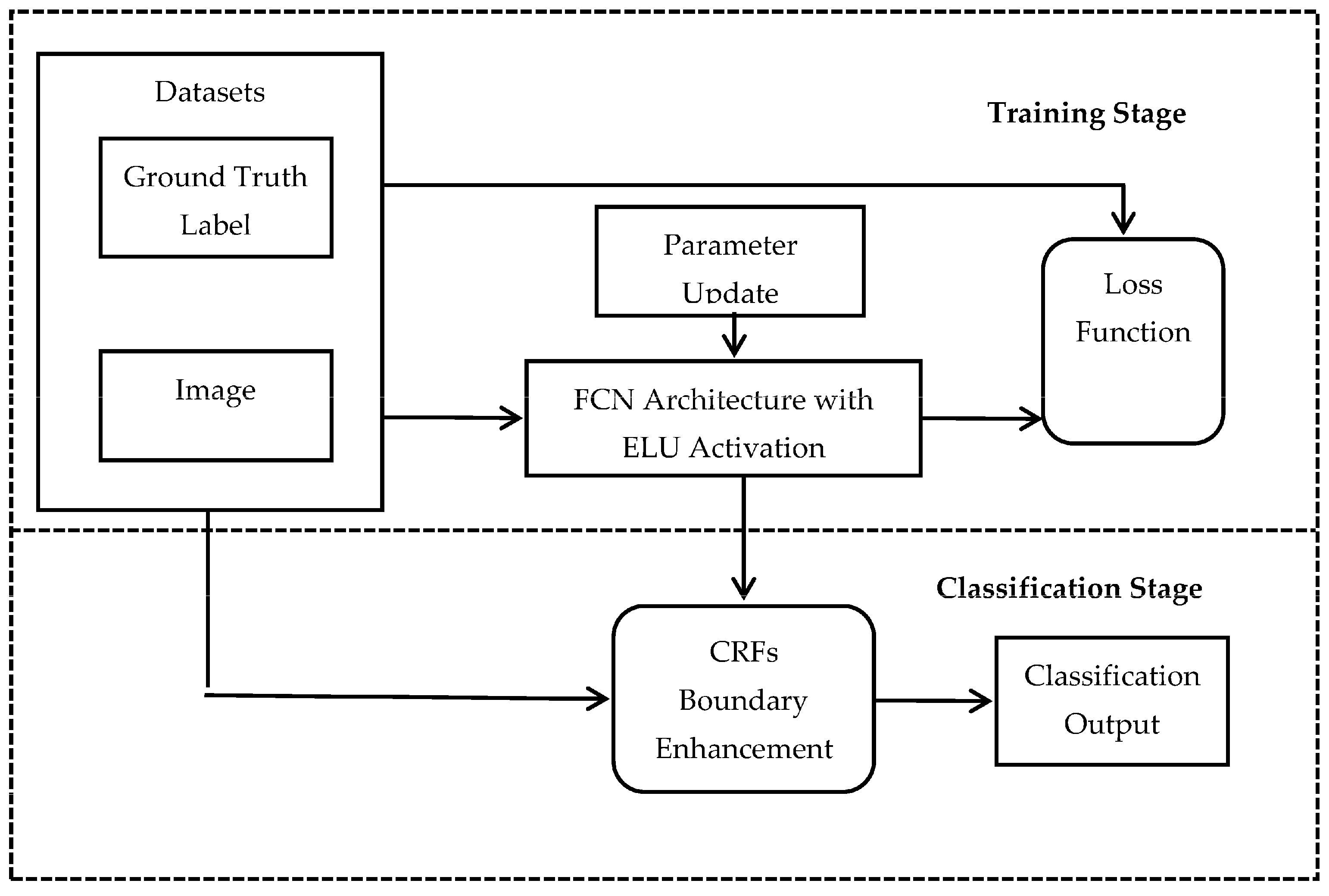
The proposed approach for building extraction, which is equivalent to classical supervised classification, has two stages, namely, a training stage and a classification stage, as shown in Figure 1. During the training stage, the image-label pair is input into the modified FCN network (ELU-FCN) as a training sample. Then, the modified FCN network predicted the class label. The error between the predicted class label and input ground-truth label (GTLabel) is calculated using the designed algorithm and backpropagated through the network using the chain rule. Then, the parameters of the modified FCN network are updated using the mini-batch gradient descent method. The mini-batch gradient descent optimization method was chosen because it possesses the advantages of both batch gradient descent and stochastic gradient descent, which makes it less noisy and more efficient than other approaches. The iteration is stopped when the loss converges. For this, a validation image-label pair is used. In the classification stage, the final trained modified FCN network is used to predict the rough class label of the input image. Then, the rough class prediction, with the input image, is inputted into the CRFs post-classification processing algorithm to generate the final refined binary classification output. The details of this method are presented below.
Network Architecture
CNN is currently a state-of-the-art technology for visual recognition tasks such as classification and detection. One of the very deep CNN networks is VGG, which was runner-up in the ImageNet Large Scale Visual Recognition Competition (ILSVRC) in 2014 [28]. Although deeper CNN networks that have recently emerged, such as ResNet [33] and Inception-V4 [22], have lower error rates in many visual recognition tasks, VGG networks have clear structures and compact memory requirements. This allows VGG to be easily extended and applied [37]. The advantages of using VGG over other networks is its simple architecture with homogenous 3 × 3 convolution kernels and 2 × 2 max pooling throughout the pipeline [38]. Among other architectures of VGG models, the VGG16 model (16-layered network) is one of the strong candidates, with an error rate of 8.5%. Therefore, we chose the VGG16 model as the baseline fixed feature extractor. Based on this, we constructed an FCN model by replacing the final three FC layers (two layers with 4096 neurons and one with 1000 neurons) by one convolutional layer. For this research, a FCN, namely, the FCN8s architecture [29], is used due to its high efficiency. Following the idea of [35], the ELU activation function is used in place of the original ReLU to increase the generalization performance during training and the accuracy of classification.
Fully Convolutional Network
The 16 layers of the selected VGG network are divided into five convolution stages, which are grouped into a pair of two or three convolutional layers, followed by three final FC layers before a softmax classifier. Going through the fully connected layers, the two-dimensional (2D) structure of the input images that is maintained by the convolutional pooling layers is lost. Therefore, the output of standard CNN after the classifier is only the one-dimensional (1D) distribution over the class, which is only suitable for ‘image-label’ mode i.e., one label for each image. Although it has large advantages in single-scene classification, as presented in studies of Hu et al. [39], it is not fruitful for remote-sensing applications. This is because a 2D dense class map is required as an output for many remote-sensing applications, e.g., building extraction. For handling this problem and maintaining the 2D properties of an image, the FCN model was implemented by replacing the last three FC layers of original VGG with their equivalent 1 × 1 convolutional layers.
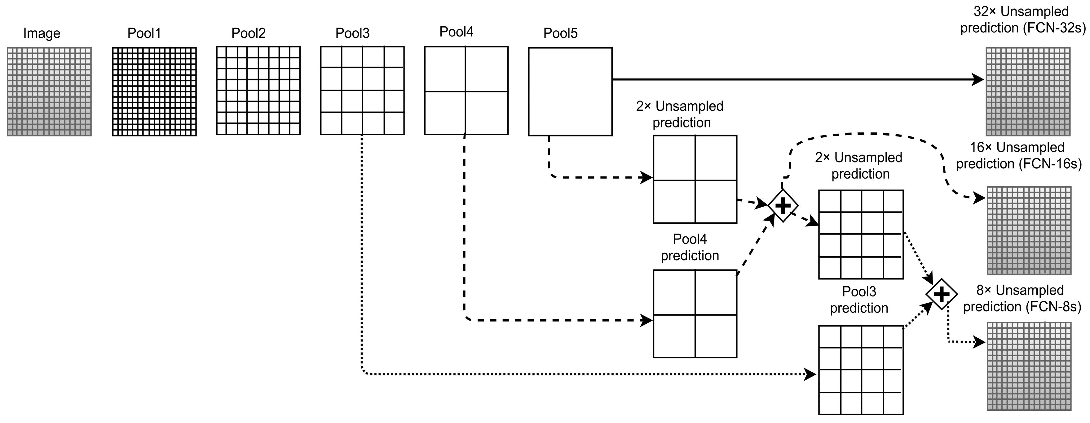
The introduction of skip connections at the end of the resulting FCN, three models were achieved as described in Long et al. [29]. Figure 2 shows that the three models that are achieved by using skip connections are FCN-8s with skip connections from the pool3 and pool4 layers, FCN-16s with skip connections from the pool4 layer, and FCN-32s without skip connections. The reasons behind using skip connections are to aggregate the features that are learned at low or medium layers to higher layers (shown on the right in Figure 2) and to help the classifier make predictions based on the aggregated features. Another major advantage of this approach is the preservation of the spatial information. The fully connected layers pairwise connect each neuron with every neuron of its preceding layer. Thus, spatial information is lost. In contrast, convolutional layers only connect each neuron to the neurons in its effective receptive field in a deep network [38]. Moreover, 140 million parameters are estimated for the final FC layers, which will be subsequently discarded by using features at the higher intermediate pooling layers. For this, additional convolutions are applied for each of the pool5, pool4, and pool3 features before feeding them into the classifier. Here, a deconvolutional layer is used to resize the final score that is predicted in the small feature space to the input image size, which allows the FCN architecture to take in images of any input size. More importantly, in the chosen designed model (FCN-8s) of FCN architecture, the feature maps at all three stages (layer 7, layer 10, and layer 13) from the VGG network are used, thereby making it more robust.
We adopted the FCN-8s model for building extraction using aerial imagery. The output number (channels) of the last convolutional layer was set equal to the number of classes that are required (for this research, it is two for building classification). The feature maps are the heat maps of the corresponding classes, which are subsequently up-sampled to match the original image size.
Network Training
The training image-ground-truth label pair are input into the modified FCN classification network as training samples. The softmax function is used to predict the class distribution in the categorical output by utilizing the output feature map that is generated by the final convolutional layer. The softmax function is a multinomial logistic function that generates a real-valued vector in the range of (0,1) that represents the categorical probability distribution for each output class [6,17,18,22,24,40].
In our case, the output of our modified FCN network is an L × B × K feature map, which has the same dimension as the original image, where L and B represent the dimensions (length and breadth) of an output of the final convolutional layer of the modified FCN network and K represents the output dimension (K = 2 in this case). X = [x1,x2]T represents the pixel value in the output of the fully convolutional layers at each location with coordinates (i,j), where 0 ≤ i ≤ L; 0 ≤ j≤ B. The softmax function is used to convert each pixel value into a 2-D class probability vector, which is denoted as m = [m1,m2]T. The following equation shows how the softmax function predicts the probability of the jth class given the sample vector X.
where W represents the weight and, b represents the bias [17,38,40].
The result of a comparison between GTLabels and the predicted label after applying the softmax function is used to calculate the cross-entropy loss. For the softmax classifier, the cross-entropy loss for each vector is the negative log likelihood of the training dataset N under the model.
where y represents a possible class, x is the data of an instance, W is the weights, b is the bias, i is the specific instance, and N represents the total number of instances [38,40].
Once the loss function has been defined, training of the CNN must be performed to extract the parameters that minimize the loss. For this case, the concept of backpropagation is used, which is the fundamental concept in learning. The mini-batch gradient descent optimization algorithm is used to update the parameters (weights and bias) of the network. This is done by computing the derivative (∂L/∂Wij) of the loss function and the derivative (∂b/∂Wij) of the bias with respect to weight wij (the weight value between neurons i, j in the two proximal layers) and the bias bi, respectively, as:
where α denotes the learning rate, which is a parameter that determines how much an update influences the current values of the weights, i.e., how much the model learns in each step.
2.1.3. Post-Classification Processing Using the Trained Network
The modified FCN network involves up-sampling operations, which results in blurring of the classification boundaries. The coupling of the classification capability of the modified FCN network with the fully connected CRFs can be one-way to produce accurate classification results in which the object boundaries are recovered at the required level of detail. Several works [18,32,36,41] used CRFs for post-processing to refine the image segmentation results. Following their strategy, we adopted the fully connected CRFs to refine our rough class prediction. This enables us to combine elegantly single-pixel prediction and shared structure through unary and pairwise terms by establishing a pairwise potential on all pairs of pixels in the remote-sensing image.
The energy function for the model is
where x represents the label assignment for each pixel and represents the pixelwise unary likelihood, which is equivalent to ), where ) is the label assignment probability at pixel i, which is computed by DCNN.
Efficient interference can be achieved by establishing the pairwise potential while using a fully connected graph, i.e., connecting all pairs of image pixels i and j. The pairwise edge potential can be defined as a linear combination of Gaussian kernels and has the form
where µ is a label compatibility function and is a Gaussian kernel, which depends on the feature (defined by f) that is extracted from pixels i and j and weighted by parameter = 1 if , and zero otherwise, as in the Potts model, which means that only nodes with distinct labels are penalized.
The kernel can be further subdivided into two parts,
where the first bilateral term is called the appearance kernel and depends on the pixel color intensities () and the pixel position (), and the second term is called the smoothness kernel, which only depends on the pixel positions. The former term encourages the assignment of a similar label to nearby pixels that have similar color intensity, while the latter term is responsible for removing small isolated regions. The hyperparameters control the scales of the Gaussian kernels. Parameter controls the degree of nearness, and the degree similarity [41].
2.2 Experimental Design and Evaluation
2.2.1. Experimental Dataset
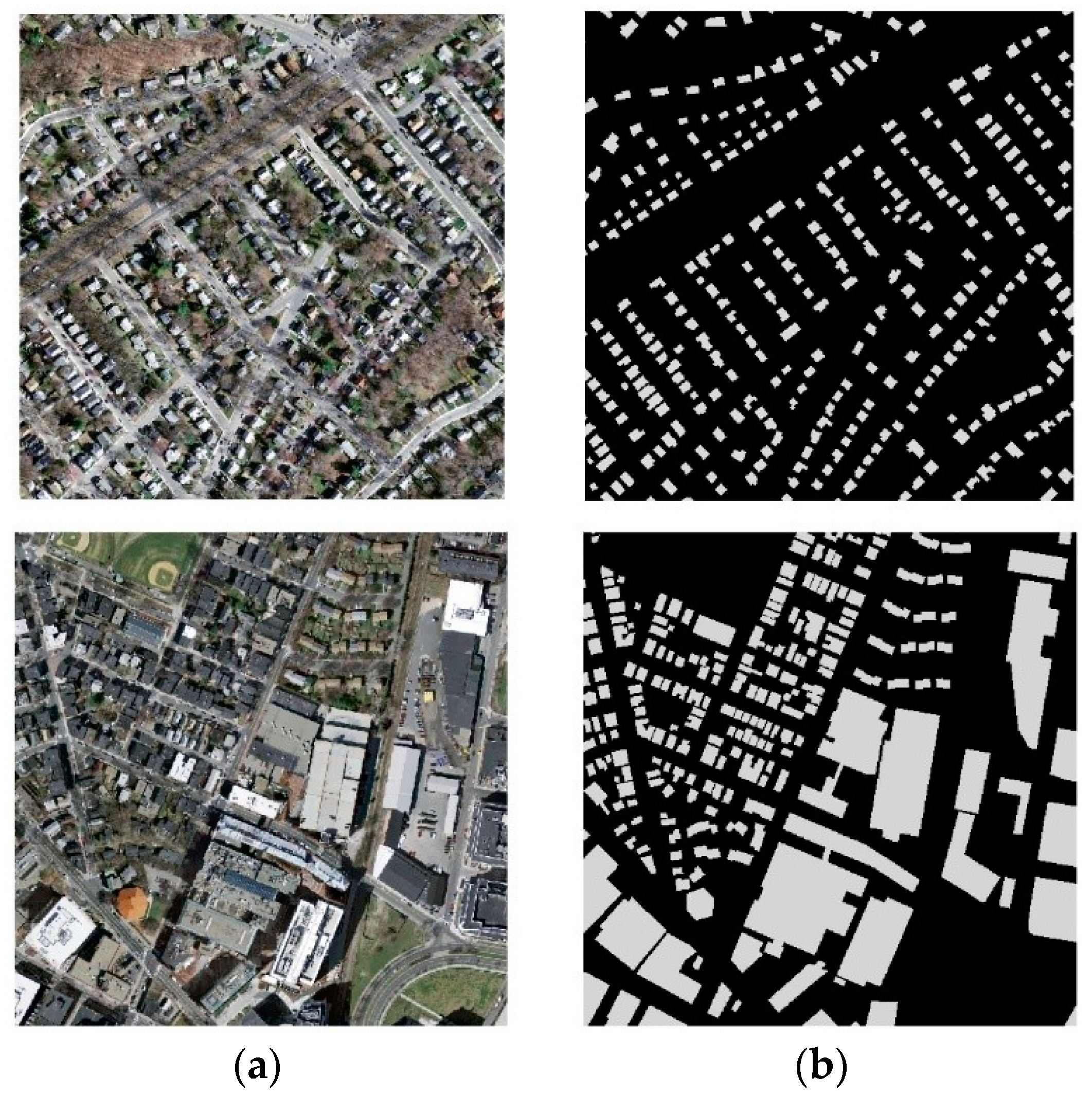
The Massachusetts building dataset that was prepared by Mhin [18] was used in this research. The dataset contained 151 images of the state of Massachusetts. Each image was a 1500 × 1500 pixel RGB image, with a spatial resolution of 1 m, covering an area of 2.25 square kilometers. The target maps that were used for the images were prepared using OpenStreetMap datasets and were also made available in rasterized format. The original images, which were of 1500 × 1500 pixel dimensions, were cropped systematically into 500 × 500 pixel-dimension. Samples from this new dataset are shown in Figure 3.
The original images were arbitrarily split into training, validation, and test datasets, with number of 137, 4, and 10, respectively. This is an original image size without considering the preprocessing. A set of images with GTLabels pair (training set) was used to train the model. The performance of the model trained by training set was then evaluated using the test set, which is also composed of a set of images and GTLabels pair. A validation set was used to determine whether the best possible model was obtained by using sensitivity experiments. Generally, this was done by using the validation set to tune the parameters of the model during training by periodically evaluating the model on the validation set. After cropping, the size of each dataset is increased ninefold.
2.2.2. Experimental Design
The experiments that were carried out in this research were mostly built on top of the deep learning framework “Tensorflow” [42]. All the experiments were conducted on a server with NVIDIA Tesla K40 of 10,968 MiB. Our main objective in the experiments was to adopt modified FCN as a classifier. As a part of the adopted CNN network, a VGG-16 network that was pre-trained on ImageNet was implemented as a feature extractor freezing 13 convolutional layers. Other layers of FCN were trained using building datasets for fast convergence. Apart from the VGG network, a constant 7 × 7 receptive field was used for networks in the fully convolutional layer at the end of the chosen network. This was devised at [29] and used in the research, keeping in mind that the average dimension of the buildings matches this dimension. A receptive field of lower dimension was not used as it takes longer to train the network. The weights were initialized randomly in each layer (apart from the frozen VGG-13 layer) with a zero-mean Gaussian distribution with a standard deviation of 0.01. For optimization of parameters during training of the network, the Adam optimization algorithm, which is based on mini-batch gradient descent, was applied. The Adam optimization algorithm was adopted due to its high performance in practice compared to other optimization algorithms such as RMSprop, Adadelta, and AdaGrad [43]. Moreover, a decrease in learning rate is automatically synchronized with the iterations in this algorithm.
Hyperparameters are the specific “higher-level” properties of the model cannot be directly learned from the regular training process and, thus, should be fixed prior to the training process [44]. The optimal value of each hyperparameter helps the CNN network discover the parameters of the model that result in robust prediction. Sensitivity analysis of the hyperparameters, namely, the learning rate, batch size, number of iterations, weight loss decay, and dropout regularization, on the performance of the chosen network were conducted to determine the optimal values of the hyperparameters, which were found to be 5, 40,000, , and 0.5, respectively. Note that number of iterations for CNN can vary depending upon the CNN architecture, and training was stopped based on the loss and accuracy graph. Similarly, to determine the optimal values for parameters for post-processing CRFs algorithm, parameter-tuning experiments were performed. The parameters that were investigated in these experiments were Gaussian kernels as components of the appearance kernel, smoothness kernel as a component of the smoothness kernel, and the total number of iterations, the optimal values of which are 3, 10, 3, and 15. These optimal values of the CNN hyperparameters and parameters for CRFs post-processing were used during training for classification.
Apart from the abovementioned experiments, two major experiments were conducted in the research. The first experiment aimed at demonstrating that each of the proposed strategies can improve the performance. First, ELU-FCN is compared to FCN for the ELU strategy. Second, ELU-FCN is compared to ELU-FCN for the CRFs strategy. Finally, we compare all variations to evaluate the significance of the combined proposed strategy. The next experiment is performed to compare the proposed method with pre-existing methods to determine the significance of the proposed method for building extraction. All the experiments that were conducted in the research were based on several approaches, which are discussed as follows.
2.2.3. Performance Evaluation
Building extraction is considered a binary problem in which building pixels are positive and the remaining non-building pixels are negative. Therefore, all performance metrics that are considered in this research are based on four classification outputs: true positive, true negative, false positive, and false negative. True positive (TP) denotes the number of target pixels (building pixels) that are correctly classified. True negative (TN) denotes the number of non-target pixels (background pixels) that are correctly classified. False positive (FP) is the number of non-target pixels that are classified as targets. False negative (FN) is the number of target pixels that are classified as non-targets. The experiments are based on several evaluation metrics: precision, recall, F1-score, and the Intersection over Union (IoU) measure. For this, the classifiers were evaluated on a test set as opposed to the true ground truth, and the resulting performance metrics for each of the classifiers were evaluated and recorded.
Precision (also known as correctness) refers to the fraction of correctly classified positive pixels (buildings) relative to all predicted positive pixels (buildings) by the classifier, whereas recall (also known as completeness) is the proportion of correctly classified positive pixels among all true target pixels. The F1-score is the weighted average of precision and recall. It takes both FP and FN into account. Another useful metric is the IoU measure, which is the average value of the intersection of the prediction and ground-truth regions over their union. The relationships among all performance metrics with the four possible classification outputs are presented as follows:
The same metric as was used by the pre-existing classifiers [10,18,25] was adopted for comparison and to evaluate the result. The averaged relaxed precision and recall scores (after this, called relaxed precision and relaxed recall), instead of the exact scores, were utilized for evaluation. The relaxed precision is defined as the fraction of predicted building pixels that are within ρ pixels of a true building pixel, while relaxed recall is defined as the fraction of true building pixels that are within ρ pixels of a predicted building pixel [24]. These are common measures for evaluating this type of prediction and are also used in [45]. For all experiments that are discussed in this research, slack parameter ρ was set to 3 pixels [10,18,25]. For the specified value of the slack parameter, a positively classified pixel is considered correct if it is within the same number of pixels from any positive pixel in the ground truth. This is a realistic approach, as the borders of buildings in the ground truth are generally some pixels off due to the generation procedure [25]. Similarly, the relaxed F1-score and relaxed IoU measure were also computed using the relaxed precision and recall.
In addition, a visual comparison of the classified building maps that were predicted by the proposed variations in the classification methods was performed. Representative parts of the study area were chosen with different complexities, structures, and numbers of buildings. The classified maps were inspected for occurrences of buildings in the predicted map and their shapes and compared to their GTLabels. Finally, the computation time that was taken by each of the classifiers during training and the complexity of each network in terms of the parameters to be learned during training were taken into consideration for comparison.
3. Results and Discussion
This section presents the details of the experiments that were conducted in the work. The first sub-section presents and discusses the findings of the comparison of the variations of the selected network. The final sub-section presents the findings of the comparison of the proposed method with the pre-existing classifiers.
3.1. Results of the Comparison of the Variations of the Proposed Classifier
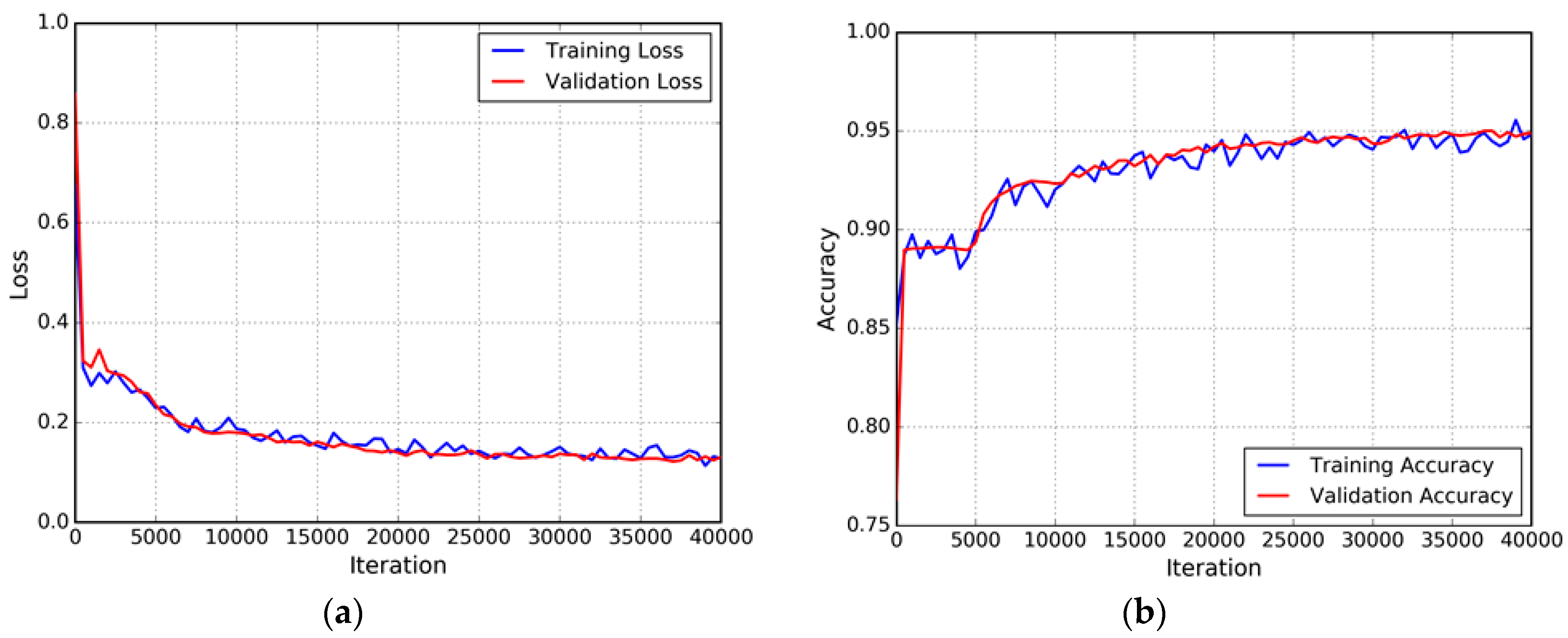
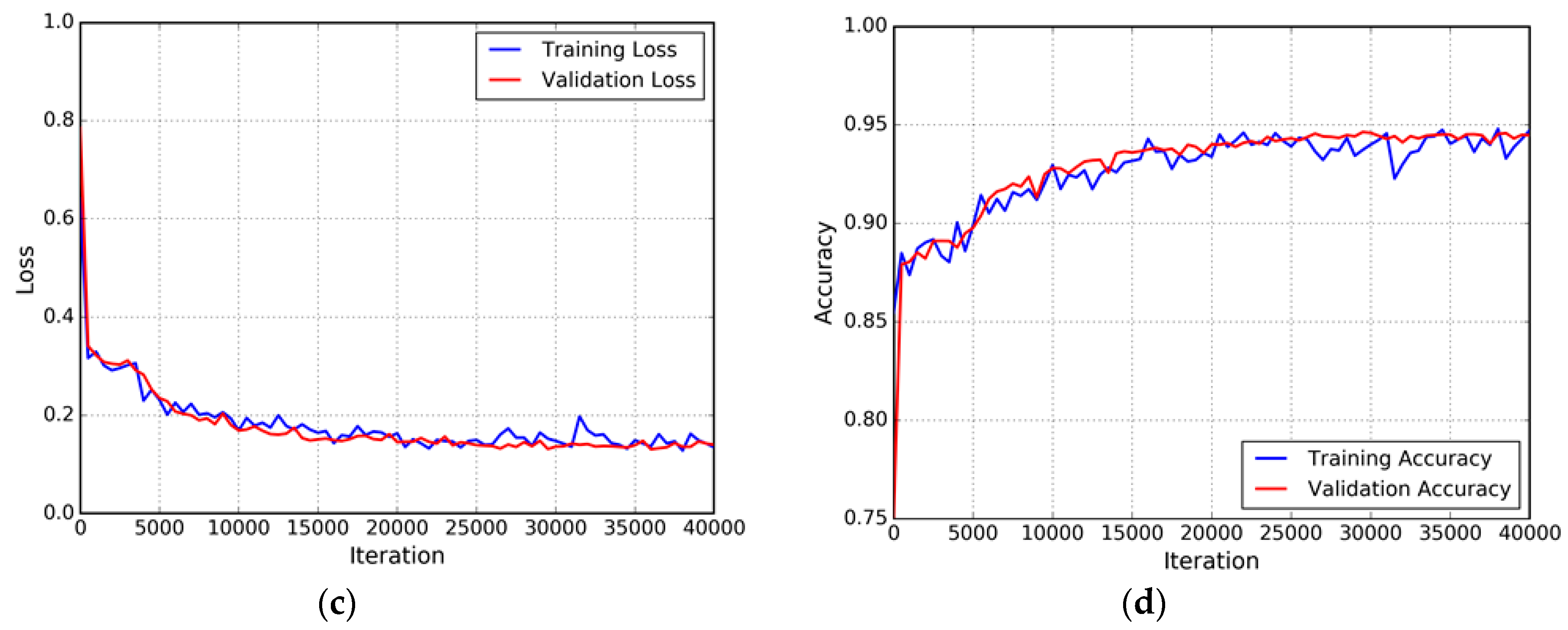
This sub-section presents the results of the experiment that was conducted on the variations of the selected classifier. To achieve high accuracy, the network must be properly configured and trained. Figure 4 shows that each model is properly set up and trained until the loss converges and the accuracy reaches the maximum value. The optimal number of iterations of the FCN-8s and ELU-FCN models is 40,000 (approximately 40 epochs).
3.1.1. Qualitative Analysis of Comparison of Variation of Proposed Classifier
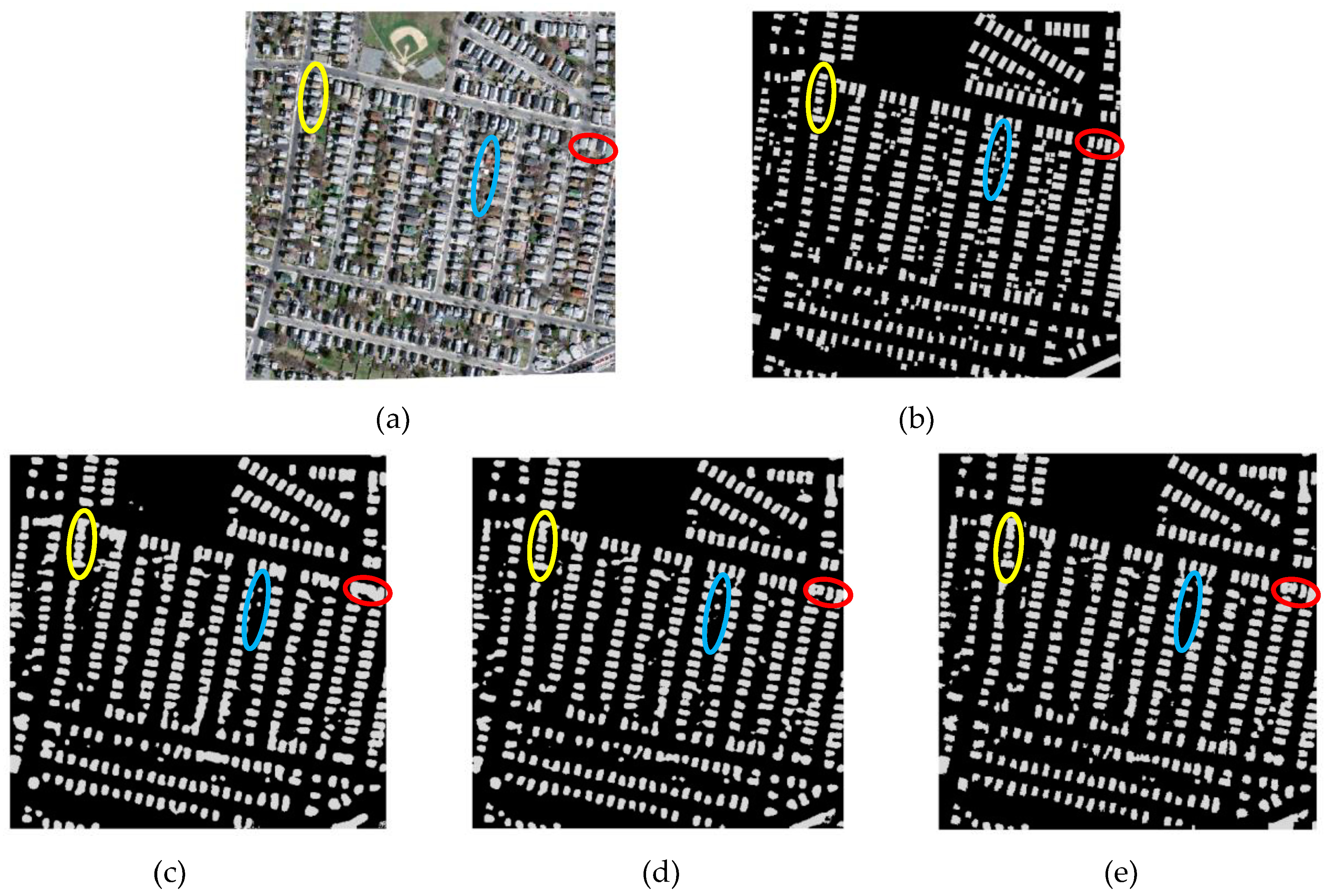
Firstly, for qualitative analysis, visual inspection and comparison of classification maps are performed by considering a representative area for the images, with a special focus on different characteristics of buildings and the surroundings. Figure 5 presents an example of an area from the Massachusetts data and the prediction results that are obtained by applying the FCN network, the modified FCN network (ELU-FCN) and the ELU-FCN in conjunction with post-processing CRFs. The predicted labels, which are shown in Figure 5c, indicate that the FCN network assigns the same class to most of the buildings, except some adjacent small buildings. They either appear as one connected region or do not appear as buildings. Figure 5d shows the predicted labels that are output after the introduction of the ELU-FCN network. This improved the quality of the predicted output compared to the base FCN network. Some of the adjacent connected buildings were well segmented by using the ELU-FCN network, but this was not valid for all the buildings. This is well demonstrated by comparing the building outputs that are encircled by the red circle, for which the introduction of ELU-FCN improved the result from the FCN network. This confirms the reason behind the small increase in the precision value when the base FCN model is improved (discussed in quantitative analysis part of this section). Furthermore, CRFs is also capable of filtering false building patches (see Figure 5e). This characteristic of CRFs helped further increase the precision of the classifier.
Many connected regions that are predicted by base FCN can be refined by neither ELU-FCN nor ELU-FCN-CRFs, especially in dense residential areas where there is little spacing between the buildings. This is demonstrated by comparing the results for the regions that are encircled in the yellow circles. This is the main reason behind the insignificant increase in the precision value after choosing ELU-FCN over FCN (discussed in quantitative analysis part of this section). Eliminating this error may require another level of segmentation to differentiate buildings from the background, as suggested by Yu et al. [46]. Similarly, smaller buildings are not well predicted by either of these classifiers. These are either not assigned the building label or joined with adjacent buildings to form a single building, which is enclosed by a blue circle. This is due to the use of the fixed receptive field (7 pixel), as explained in detail in [29].
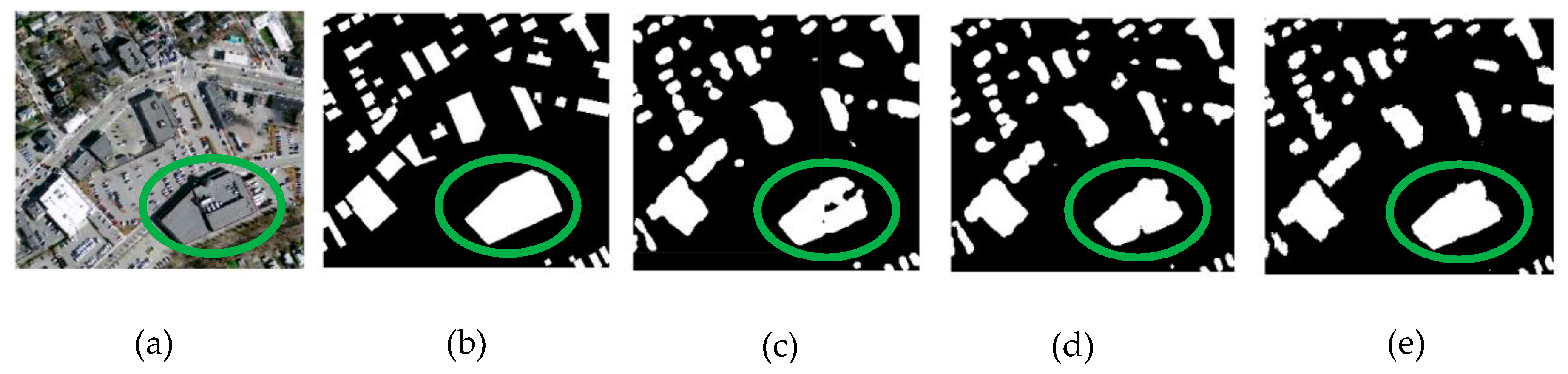
The FCN network produced irregular building outlines compared to the ground truth for both small and large buildings. Little enhancement of the boundaries of the buildings is achieved by adopting ELU-FCN. However, the introduction of post-processing CRFs enables the further refinement of the shapes of the buildings. This is demonstrated in Figure 6 in the area enclosed by the green circle.
In summary, it is concluded that the performance of models in predicting large buildings is better than that in predicting the smallest buildings but less accurate compared to the medium-sized buildings. The main reason behind this is the use of the constant receptive field. In addition, although no significant improvement by using post-processing CRFs is identified in the quantitative analysis, the qualitative results indicate improved performance, especially in cases of edge enhancement of buildings and refinement of large buildings. Low improvement in the quantitative measures can be attributed to the poor performance on small and nearby buildings, which cover a major part of the study area.
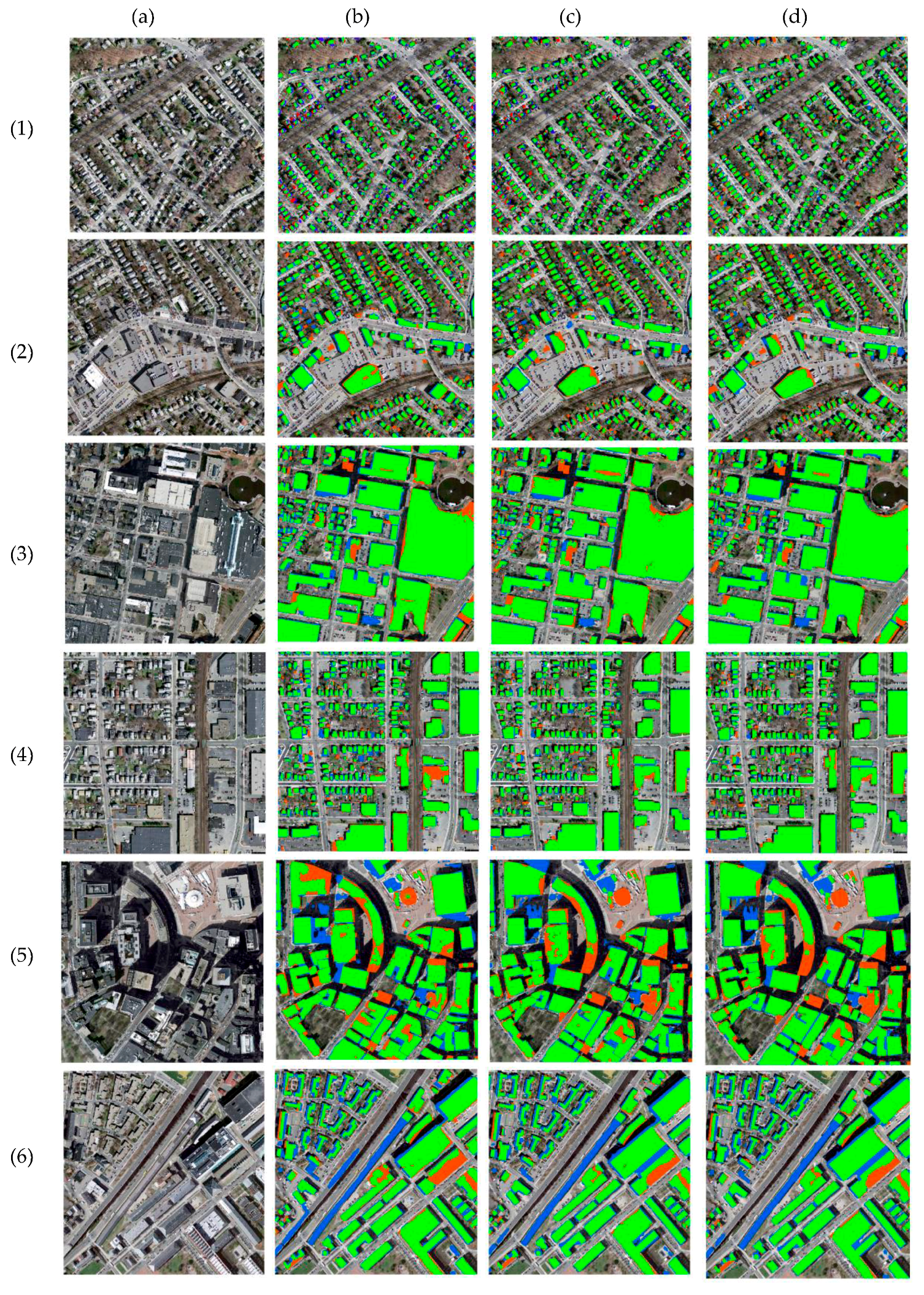
To obtain deep insight into the model performance and to interpret the quantitative measures of performance, we visualized the prediction results of three networks. These further analyses the ability of the network to extract buildings with variations in appearance, size, occlusion, and denseness. The representative images are chosen from the test dataset and the predictions from the three networks are visualized. Figure 7 illustrates the predictions on the parts of the test set by color coding, in which the colors indicate whether the prediction is true or false.
The progression from left to right in each row in Figure 7 suggests that the proposed methods performed well with modification of the base FCN network. The figures also suggest that the network performs well at detecting buildings of multiple sizes with different appearances and under different circumstances (shown in green), whether in areas with large high-rise buildings, residential areas, or industrial areas, the FP (shown as blue pixels) and FN (shown as red pixels) of the predicted labels show several failure cases for our proposed model and illustrate several problems with the data. The network is penalized for making a building prediction where there is a building in the image but not in the ground truth, which appears in the prediction as a FP. Moreover, small adjacent buildings appear as a connected region, which gives rise to FP in the spaces between buildings. This is because of the small spacing between buildings and the shadows that are cast by buildings on the spaces between them. The majority of the buildings that are classified as FN in the predicted label are smaller buildings, which can be attributed to the use of the constant receptive field of the network. The FN for some large buildings are also due to the use of the constant receptive field. Other reasons for FN are the shadows of tall buildings and tree cover over the buildings.
Table 2 shows the resulting F1-score for each patch of images. The F1-score of the proposed method (ELU-FCN-CRFs) is higher than those of FCN and ELU-FCN for almost every patch of images. That of ELU-FCN-CRFs is superior to that of ELU-FCN by only 0.03%. However, there is a much larger improvement in F1-score for ELU-FCN-CRFs than for FCN by a margin of 1.1%.
3.1.2. Quantitative Analysis of Comparison of Proposed Classifier
The results of quantitative analysis of comparison between the baselines (FCN) and other variations of the proposed techniques is presented in Table 3. Our proposed network with all strategies (ELU-FCN-CRFs) outperforms the other methods. More details are discussed below to show that each of the proposed techniques can improve the accuracy.
Results of Enhanced FCN (ELU-FCN)
Our first strategy aims at increasing the accuracy of the network by using ELU as an activation function (used in ELU-FCN) rather than the traditional ReLU (used in FCN). Table 3 shows that ELU-FCN (93.81%) outperforms the original FCN (93.09%) in terms of F1-score, with an increase of approximately 1%. There is also an improvement in IoU measure from 86.96% to 88.93% by choosing ELU-FCN. This increase in F1-score and IoU measure is mainly due to the higher increase in recall. The increase in recall (approximately 2%) for ELU-FCN signifies the increased robustness of modified FCN in predicting the buildings. However, the precision value is stagnant, which suggests that modified FCN did not significantly contribute to eliminating the noise in the prediction of the FCN network. In both models, the precision value is always greater than the recall value. This signifies that the model identifies fewer false buildings while failing to predict the correct buildings. This is mostly due to the model’s weakness in predicting smaller buildings. This suggests that ELU is more robust than ReLU in detecting building pixels. The experiment confirms that the use of ELU enhances the performance of the CNN classifier.
Results of Post-Processing CRFs (ELU-FCN-CRFs) on Enhanced FCN (ELU-FCN)
Further improvement is achieved by integrating CRFs into the modified network, as discussed earlier. The strategy uses CRFs to sharpen the building boundaries and filter false building patches. Table 3 shows that the F1-score of ELU-FCN-CRFs (93.93%) is superior to that of ELU-FCN (93.81%). Similarly, in terms of IoU value, this combined method (89.08%) slightly exceeds ELU-FCN (88.93%), with an increase of 0.1%. The increase in F1-score and IoU value compared to ELU-FCN is mostly attributes to an increase in precision (an increase of 0.4%), with no change in recall value. This signifies that post-processing CRFs refine the noise that is produced by ELU-FCN. However, the constant value of recall signifies that CRFs is not able to recover the building pixels. Additionally, the precision value is greater than the recall value for both models than for previous models. It is concluded from this experiment that a small but not significant improvement is obtained by adding the post-processing CRFs, which is in accordance with the experiments that were conducted in [29] numerically.
Combined Results All Variation of Networks
The combined results indicate that the F1-score of ELU-FCN-CRFs (93.93%) is superior to that of FCN (93.09%). Similarly, in terms of IoU value, the combined method (89.08%) outperforms FCN (86.96%), with an increase of 2.1%. These increases in F1-measure and IoU value are attributed to increases in both precision and recall values compared to the original FCN network. This suggests that improved FCN can reduce false detections of buildings and increase the sensitivity of the network. Thus, we conclude that the combined method achieves a significant improvement over the base FCN network.
3.1.3. Comparison of Variation of Proposed Classifier on Network Complexity
The variations in the proposed techniques are also compared in terms of computation time and network complexity. All the analyses with the various classifiers were run on an NVIDIA Tesla K40 of 10,968 MiB. There is no significant effect on computational time due to changing the activation function from the traditional ReLU activation function to the ELU activation function. Both took approximately 21 h to train in up to 40,000 iterations. The addition of CRFs post-processing increased the computational time by approximately half an hour in choosing the ELU-ECN-CRFs classifier. In terms of complexity, FCN and ELU-FCN are equally complex with the same series of convolutional layers followed by nonlinear activation and pooling operations. Post-processing CRFs adds some complexity but far less compared to CNN networks.
3.2. Results of Comparison of the Proposed Method with Pre-Existing Classifiers
Table 4 shows the results of different models, including our approach, on the Massachusetts building datasets. Note that the proposed method has been implemented and tested on an experimental dataset, whereas the results for the other three are adopted from an original published paper [10]. The results show that our proposed method is superior to all other methods except that of [10] in terms of F1-score. Our proposed method yields a higher F1-score than those of [18] and [25], at 1.82% and 1.63%, respectively, but lags behind the result from [10] by a margin of only 0.3%. All of the variations of the proposed model achieve superior performance in terms of F1-score compared to the results from [18] and [25].
Apart from performance measures, it is worth comparing the models based on computational complexity. The complexity of the CNN network is generally associated with the number of parameters to be learned during training. The CNN-based classifier that was used by Mhin [18] and Saito et al. [25] contains only three convolutional layers followed by two FC layers. There is a tremendous increase in the number of parameters to be learned during training when using the network that was proposed by Marcu and Leordeanu [10]. This is because it combines VGG-16 with Alex-Net and adds an extra three FC layers at the end. An FCN has parameters that are equivalent to only one FC layer in place of 3 FC layers of VGG-16. This implies that the FCN network has a convolutional network of 13 layers and an equivalent layer to one FC layer. Thus, considering the complexity of the network, the classifier that was used by Mnih [18] and Saito et al. [25] is the least complex. The FCN network is slightly more complex than the previous one due to a larger number of convolutional networks (13 compared to 3). However, the CNN network that was adopted by Marcu and Leordeanu [10] is far more complex due to the combination of two individual networks that each have the same or higher complexity compared to FCN, with more FC layers at the end.
4. Conclusions and Future Works
The main objective of this research is to develop a new method that exploits the deep-learning-based CNN approach to learn from aerial images for building extraction. A FCN is chosen among other available networks for semantic segmentation due to its balance between accuracy and network complexity. The original FCN model is modified by introducing an ELU in place of a ReLU to accelerate learning and obtain high classification accuracy. Additionally, a post-classification processing approach, namely CRFs, is implemented to enhance the boundaries of buildings and further increase the performance. The experiments were conducted on a Massachusetts building dataset. The preliminary results of the comparison of variations of the proposed method suggest that our proposed ELU-FCN-CRFs outperforms the original and other variations of proposed methods on aerial imagery. This result indicates that the proposed technique can enhance the accuracy. The results of the comparison of the proposed method with other pre-existing classifiers show that our proposed method achieves superior performance in terms multiple performance measures and network complexity.
In the future, for the model that was developed in this research, hierarchical adaptation of the receptive field is one option for increasing the accuracy, as our results found the use of the constant receptive field to be one of the major causes of the loss in accuracy. Additional semantic segmentation, optimization, and/or post-processing techniques can be explored and compared to obtain the best framework for building extraction.
Author Contributions
The experiment design as well as result analysis was carried out by S.S.; L.V. supervised research and reviewed results. The article was co-written by both authors. All authors read and approved the submitted manuscript.
Funding
This research received no external funding.
Acknowledgments
This paper is a part of masters’ thesis submitted as a part of partial fulfillment of the Master of Science in Geospatial Technologies. Shrestha S. thanks Erasmus Mundus program for funding the studies. We greatly acknowledge LIP-Laboratório de Instrumentação e Física Experimental de Partículas for their untiring effort and help during accessing server for simulation for the thesis.
Conflicts of Interest
The author declares no conflict of interest.
Abbreviations
The following abbreviations are used in the manuscript.
| CNN | Convolutional Neural Network |
| CRFs | Conditional Random Fields |
| DCNN | Deep Convolutional Neural Network |
| ELU | Exponential Linear Unit |
| FCN | Fully Convolutional Network |
| FN | False Negative |
| FP | False Positive |
| GTLabel | Ground Truth Label |
| IoU | Intersection Over Union |
| NRG | Near Infrared, Red, Blue |
| PASCAL VOC | PASCAL Visual Object Classes |
| PCA | Principal Component Analysis |
| ReLU | Rectified Linear Unit |
| RGB | Red, Green, Blue |
| SVM | Support Vector Machine |
| TN | True Negative |
| TP | True Positive |
| VGI | Volunteered Geographic Information |
References
- Planet. Planet Doubles Sub-1 Meter Imaging Capacity with Successful Launch of 6 Skysats. Available online: https://www.planet.com/pulse/planet-doubles-sub-1-meter-imaging-capacity-with-successful-launch-of-6-skysats/ (accessed on 22 December 2017).
- Digital Globe. Open Data for Disaster Recovery. Available online: https://www.digitalglobe.com/ (accessed on 12 November 2017).
- FAA. UAS Integration Pilot Program. Available online: https://www.faa.gov/uas/programs_partnerships/uas_integration_pilot_program/ (accessed on 12 November 2017).
- Space News. U.S. Government Eases Restrictions on DigitalGlobe. Available online: http://spacenews.com/40874us-government-eases-restrictions-on-digitalglobe/ (accessed on 12 December 2017).
- Mayer, H. Automatic object extraction from aerial imagery—A survey focusing on buildings. Comput. Vis. Image Underst. 1999, 74, 138–149. [Google Scholar] [CrossRef]
- Krizhevsky, A.; Hinton, G.E. Imagenet classification with deep convolutional neural networks. Adv. Neural Inf. Process. Syst. 2012, 1, 1097–1105. [Google Scholar] [CrossRef]
- Shu, Y. Deep Convolutional Neural Networks for Object Extraction from High Spatial Resolution Remotely Sensed Imagery. Ph.D. Thesis, University of Waterloo, Waterloo, ON, Canada, 2014. [Google Scholar]
- Yuan, J. Automatic building extraction in aerial scenes using convolutional networks. arXiv, 2016; arXiv:1602.06564. [Google Scholar]
- Nielsen, J. Participation Inequality: Encouraging More Users to Contribute, Alertbox. Available online: http: //www. useit.com/alertbox/participation_inequality fifth (accessed on 22 July 2017).
- Marcu, A.; Leordeanu, M. Dual local-global contextual pathways for recognition in aerial imagery. arXiv, 2016; arXiv:1605.05462. [Google Scholar]
- Yuan, J.; Cheriyadat, A.M. Learning to count buildings in diverse aerial scenes. In Proceedings of the 22nd ACM SIGSPATIAL International Conference on Advances in Geographic Information Systems, Fort Worth, TX, USA, 4–7 November 2014; pp. 271–280. [Google Scholar]
- Huertas, A. Detecting buildings in aerial images. Comput. Vis. Graph. Image Process. 1998, 41, 131–152. [Google Scholar] [CrossRef]
- Peng, J.; Liu, Y.C. Model and context—Driven building extraction in dense urban aerial images. Int. J. Remote Sens. 2005, 26, 1289–1307. [Google Scholar] [CrossRef]
- Levitt, S.; Aghdasi, F. An investigation into the use of wavelets and scaling for the extraction of buildings in aerial images. In Proceedings of the IEEE 1998 South African Symposium on Communications and Signal Processing, Rondebosch, South Africa, 8 September 1998; pp. 133–138. [Google Scholar]
- Inglada, J. Automatic recognition of man-made objects in high resolution optical remote sensing images by SVM classification of geometric image features. ISPRS J. Photogramm. Remote Sens. 2007, 62, 236–248. [Google Scholar] [CrossRef]
- Sumer, E.; Turker, M. An adaptive fuzzy-genetic algorithm approach for building detection using high-resolution satellite images. Comput. Environ. Urban Syst. 2013, 39, 48–62. [Google Scholar] [CrossRef]
- Alshehhi, R.; Reddy, P.; Lee, W.; Dalla, M. Simultaneous extraction of roads and buildings in remote sensing imagery with convolutional neural networks. ISPRS J. Photogramm. Remote Sens. 2017, 130, 139–149. [Google Scholar] [CrossRef]
- Mnih, V. Machine Learning for Aerial Image Labeling. Ph.D. Thesis, University of Toronto, Toronto, ON, Canada, 2013. [Google Scholar]
- Vakalopoulou, M.; Karantzalos, K.; Komodakis, N.; Paragios, N. Building detection in very high resolution multispectral data with deep learning features. In Proceedings of the IEEE International Geoscience and Remote Sensing Symposium, Milan, Italy, 26–31 July 2015; pp. 1873–1876. [Google Scholar]
- Bittner, K.; Cui, S.; Reinartz, P.; Vi, C.; Vi, W.G. Building extraction from remote sensing data using fully convolutional networks. Int. Arch. Photogramm. Remote Sens. Spat. Inf. Sci. 2017, 42, 481–486. [Google Scholar] [CrossRef]
- Lin, M.; Chen, Q.; Yan, S. Network in network. arXiv, 2013; arXiv:1312.4400. [Google Scholar]
- Szegedy, C.; Liu, W.; Jia, Y.; Sermanet, P.; Reed, S.; Anguelov, D.; Arbor, A. Going deeper with convolutions. In Proceedings of the IEEE Conference on Computer Vision and Pattern Recognition, Boston, MA, USA, 7–12 June 2015; pp. 1–9. [Google Scholar]
- He, K.; Xiangyu, Z.; Shaoqing, R.; Jian, S. Delving deep into rectifiers: Surpassing Human-Level Performance on ImageNet Classification. In Proceedings of the IEEE International Conference on Computer Vision, Santiago, Chile, 7–13 December 2015; pp. 1026–1034. [Google Scholar]
- Saito, S.; Aoki, Y. Building and road detection from large aerial imagery. SPIE/IS&T Electron. Imaging 2015, 9405, 3–14. [Google Scholar]
- Saito, S.; Takayoshi, Y.; Yoshimitsu, A. Multiple object extraction from aerial imagery with convolutional neural networks. Electron. Imaging 2016, 60, 1–9. [Google Scholar] [CrossRef]
- Huang, Z.; Guangliang, C.; Hongzhen, W.; Haichang, L.; Limin, S.; Chunhong, P. Building extraction from multi-source remote sensing images via deep deconvolution neural networks. In Proceedings of the IEEE International Geoscience and Remote Sensing Symposium (IGARSS), Beijing, China, 10–15 July 2016; pp. 1835–1838. [Google Scholar]
- Maggiori, E.; Member, S.; Tarabalka, Y.; Charpiat, G.; Alliez, P. Convolutional neural networks for large-scale remote-sensing image classification. IEEE Trans. Geosci. Remote Sens. 2017, 55, 645–657. [Google Scholar] [CrossRef]
- Simonyan, K.; Zisserman, A. Very deep convolutional networks for large-scale image recognition. arXiv, 2014; arXiv:1409.1556. [Google Scholar]
- Long, J.; Shelhamer, E.; Darrell, T. Fully convolutional networks for semantic segmentation. In Proceedings of the IEEE Conference on Computer Vision and Pattern Recognition, Boston, MA, USA, 7–12 June 2015; pp. 3431–3440. [Google Scholar]
- Liu, Z.; Li, X.; Luo, P.; Loy, C.C.; Tang, X. Deep learning markov random field for semantic segmentation. IEEE Trans. Pattern Anal. Mach. Intell. 2017, 40, 1–14. [Google Scholar] [CrossRef] [PubMed]
- Noh, H.; Hong, S.; Han, B. Learning deconvolution network for semantic segmentation. In Proceedings of the IEEE International Conference on Computer Vision, Santiago, Chile, 7–13 December 2015; pp. 1520–1528. [Google Scholar]
- Chen, L.; Papandreou, G.; Member, S.; Kokkinos, I.; Murphy, K.; Yuille, A.L. DeepLab: Semantic image segmentation with deep convolutional nets, atrous convolution, and fully connected crfs. arXiv, 2016; arXiv:1606.00915. [Google Scholar] [CrossRef] [PubMed]
- He, K.; Sun, J.; Zhang, X.; Ren, S. Deep residual learning for image recognition. In Proceedings of the IEEE Conference on Computer Vision and Pattern Recognition, Las Vegas, NV, USA, 27–30 June 2016; pp. 770–778. [Google Scholar]
- Badrinarayanan, V.; Kendall, A.; Cipolla, R.; Member, S. SegNet: A deep convolutional encoder-decoder architecture for image segmentation. arXiv, 2015; arXiv:1511.00561. [Google Scholar]
- Clevert, D.-A.; Unterthiner, T.; Hochreiter, S. Fast and accurate deep network learning by exponential linear units (ELUs). arXiv, 2015; arXiv:1511.07289. [Google Scholar]
- Krahenbuhl, P.; Koltun, V. Efficient inference in fully connected crfs with gaussian edge potentials. Adv. Neural Inf. Process. Syst. 2011, 24, 109–117. [Google Scholar]
- Fu, G.; Liu, C.; Zhou, R.; Sun, T.; Zhang, Q. Classification for high resolution remote sensing imagery using a fully convolutional network. Remote Sens. 2017, 9, 498. [Google Scholar] [CrossRef]
- Muruganandham, S. Semantic segmentation of satellite images using deep learning. Master’s Thesis, Lulea University of Technology, Luleå, Sweden, 2016. [Google Scholar]
- Hu, F.; Xia, G.-S.; Hu, J.; Zhang, L. Transferring deep convolutional neural networks for the scene classification of high-resolution remote sensing imagery. Remote Sens. 2015, 7, 14680–14707. [Google Scholar] [CrossRef]
- Nogueira, K.; Penatti, O.A.B.; dos Santos, J.A. Towards better exploiting convolutional neural networks for remote sensing scene classification. Pattern Recognit. 2017, 61, 539–556. [Google Scholar] [CrossRef] [Green Version]
- Shotton, J.; Winn, J.; Rother, C. Textonboost for image understanding: Multi-class object recognition and segmentation by jointly modeling texture, layout, and context. Int. J. Comput. Vis. 2009, 81, 2–23. [Google Scholar] [CrossRef]
- Tensorflow. An Open-Source Machine Learning Framework for Everyone. Available online: https://www.tensorflow.org/ (accessed on 11 September 2017).
- Ruder, S. An overview of gradient descent optimization algorithms. arXiv, 2016; arXiv:1609.04747. [Google Scholar]
- Bergstra, J.; Bengio, Y. Random search for hyper-parameter optimization. J. Mach. Learn. Res. 2012, 13, 281–305. [Google Scholar]
- Wiedemann, C.; Heipke, C.; Mayer, H.; Jamet, O. Empirical evaluation of automatically extracted road axes. In Empirical Evaluation Techniques in Computer Vision; IEEE Computer Society Press: Washington, DC, USA, 1998; pp. 172–187. [Google Scholar]
- Yu, H.; Yang, W.; Xia, G.-S.; Liu, G. A color-texture-structure descriptor for high-resolution satellite image classification. Remote Sens. 2016, 8, 259. [Google Scholar] [CrossRef]
Figure 1.
General pipelines of our proposed approach: the training stage and the classification stage.
Figure 1.
General pipelines of our proposed approach: the training stage and the classification stage.

Figure 2.
Visualization of the VGG-FCN architecture. The figure depicts the skip connection architecture that was devised in [29]. Only the pooling and prediction layers are shown, omitting the intermediate convolutional layer. The image shows the FCN-32s variant (without skip connections) on top, the FCN-16s variant in the middle and FCN-8s variant at the bottom.

Figure 3.
Two sample aerial images from the Massachusetts building dataset; each row contains an original image on the left, which acts as a ground truth of the corresponding image on the right: (a) aerial image, (b) building mask.
Figure 3.
Two sample aerial images from the Massachusetts building dataset; each row contains an original image on the left, which acts as a ground truth of the corresponding image on the right: (a) aerial image, (b) building mask.

Figure 4.
Iteration plot on the Massachusetts satellite data sets of variations of the proposed methods: fully convolutional network (FCN) and ELU-FCN. The x-axis corresponds to the number of iterations, and the y-axis refers to the measure. Each row refers to a different model. (a) plot of model loss (cross-entropy) on the training and validation datasets for FCN ; (b) plot of accuracy on the training and validation datasets for FCN; (c) plot of model loss on the training and validation datasets for ELU-FCN; and (d) plot of accuracy on the training and validation datasets for ELU-FCN.


Figure 5.
Visual comparison of three variations of the proposed techniques using sample aerial test images of the Massachusetts area. (a) original input image; (b) ground-truth map; (c) output of FCN-8s; (d) output of ELU-FCN; and (e) output of ELU-FCN-CRFs.
Figure 5.
Visual comparison of three variations of the proposed techniques using sample aerial test images of the Massachusetts area. (a) original input image; (b) ground-truth map; (c) output of FCN-8s; (d) output of ELU-FCN; and (e) output of ELU-FCN-CRFs.

Figure 6.
Visual comparison of three variations of the proposed techniques on large buildings using sample aerial test images of the Massachusetts area. (a) original input image; (b) ground-truth map; (c) output of FCN-8s; (d) output of ELU-FCN; and (e) output of ELU-FCN-CRF.
Figure 6.
Visual comparison of three variations of the proposed techniques on large buildings using sample aerial test images of the Massachusetts area. (a) original input image; (b) ground-truth map; (c) output of FCN-8s; (d) output of ELU-FCN; and (e) output of ELU-FCN-CRF.

Figure 7.
Visualization of predictions of three variations of the proposed model on building detection tasks with original extracted test images from the Massachusetts dataset. (a) input images; (b) results of base FCN network; (c) results of ELU-FCN; and (d) results of ELU-FCN-CRFs. Green pixels are TP, red pixels are FN, blue pixels are FP, and background pixels are TN.


Table 1.
Variations in selected convolutional neural network (CNN) models: exponential linear unit (ELU) activation function and conditional random fields (CRFs).
Table 1.
Variations in selected convolutional neural network (CNN) models: exponential linear unit (ELU) activation function and conditional random fields (CRFs).
| Method | Abbreviation | Description |
|---|---|---|
| Selected network | FCN | Fully convolutional network |
| Variation of selected network | ELU-FCN | FCN + ELU activation |
| Proposed method | ELU-FCN-CRFs | FCN + ELU activation + CRFs |
Table 2.
F1-scores (%) of variations of the proposed techniques in selected regions of test images.
| Image ID | 1 | 2 | 3 | 4 | 5 | 6 | Mean |
|---|---|---|---|---|---|---|---|
| FCN | 97.13 | 95.22 | 95.06 | 97.64 | 91.05 | 88.48 | 94.09 |
| ELU-FCN | 97.79 | 95.33 | 97.70 | 98.31 | 91.36 | 90.44 | 95.16 |
| ELU-FCN-CRFs | 97.89 | 95.36 | 97.69 | 98.37 | 91.38 | 90.45 | 95.19 |
Table 3.
Results on the testing data of Massachusetts aerial images for the variations of our proposed techniques in terms of precision (%), recall (%), F1-score (%), and IoU (%).
Table 3.
Results on the testing data of Massachusetts aerial images for the variations of our proposed techniques in terms of precision (%), recall (%), F1-score (%), and IoU (%).
| Models | Precision | Recall | F1-Score | IoU | |
|---|---|---|---|---|---|
| Baseline | FCN | 94.76 | 91.63 | 93.09 | 86.96 |
| Proposed Method | ELU-FCN | 94.79 | 93.42 | 93.81 | 88.93 |
| ELU-FCN-CRFs | 95.07 | 93.40 | 93.93 | 89.08 |
© 2018 by the authors. Licensee MDPI, Basel, Switzerland. This article is an open access article distributed under the terms and conditions of the Creative Commons Attribution (CC BY) license (http://creativecommons.org/licenses/by/4.0/).
Share and Cite
MDPI and ACS Style
Shrestha, S.; Vanneschi, L. Improved Fully Convolutional Network with Conditional Random Fields for Building Extraction. Remote Sens. 2018, 10, 1135. https://0-doi-org.brum.beds.ac.uk/10.3390/rs10071135
AMA Style
Shrestha S, Vanneschi L. Improved Fully Convolutional Network with Conditional Random Fields for Building Extraction. Remote Sensing. 2018; 10(7):1135. https://0-doi-org.brum.beds.ac.uk/10.3390/rs10071135
Chicago/Turabian StyleShrestha, Sanjeevan, and Leonardo Vanneschi. 2018. "Improved Fully Convolutional Network with Conditional Random Fields for Building Extraction" Remote Sensing 10, no. 7: 1135. https://0-doi-org.brum.beds.ac.uk/10.3390/rs10071135
Note that from the first issue of 2016, this journal uses article numbers instead of page numbers. See further details here.