Article

Spatial and Temporal Dependency of NDVI Satellite Imagery in Predicting Bird Diversity over France

by
Sébastien Bonthoux
1,†,
Solenne Lefèvre
2,
Pierre-Alexis Herrault
3 and
David Sheeren
2,*,†
1
UMR CNRS 7324 CITERES, Ecole de la Nature et du Paysage-INSA Centre Val de Loire, 41000 Blois, France
2
DYNAFOR, University of Toulouse, INRA, 31321 Castanet-Tolosan, France
3
LIVE, University of Strasbourg, 67000 Strasbourg, France
*
Author to whom correspondence should be addressed.
These authors contributed equally to this work.
Submission received: 5 June 2018 / Revised: 14 July 2018 / Accepted: 16 July 2018 / Published: 18 July 2018

Abstract

:
Continuous-based predictors of habitat characteristics derived from satellite imagery are increasingly used in species distribution models (SDM). This is especially the case of Normalized Difference Vegetation Index (NDVI) which provides estimates of vegetation productivity and heterogeneity. However, when NDVI predictors are incorporated into SDM, synchrony between biological observations and image acquisition must be questionned. Due to seasonal variations of NDVI during the year, landscape patterns of habitats are revealed differently from one date to another leading to variations in models’ performance. In this paper, we investigated the influence of acquisition time period of NDVI to explain and predict bird community patterns over France. We examined if the NDVI acquisition period that best fit the bird data depends on the dominant land cover context. We also compared models based on single time period of NDVI with one model built from the Dynamic Habitat Index (DHI) components which summarize variations in vegetation phenology throughout the year from the fraction of radiation absorbed by the canopy (fPAR). Bird species richness was calculated as response variable for 759 plots of 4 km 2 from the French Breeding Bird Survey. Bird specialists and generalists to habitat were considered. NDVI and DHI predictors were both derived from MODIS products. For NDVI, five time periods in 2010 were compared, from late winter to begin of autumn. A climate predictor was also used and Generalized Additive Models were fitted to explain and predict bird species richness. Results showed that NDVI-based proxies of dominant habitat identity and spatial heterogeneity explain more bird community patterns than DHI-based proxies of annual productivity and seasonnality. We also found that models’ performance was both time and context-dependent, varying according to the bird groups. In general, best time period of NDVI did not match with the acquisition period of bird data because in case of synchrony, differences in habitats are less pronounced. These findings suggest that the most powerful approach to estimate bird community patterns is the simplest one. It only requires NDVI predictors from a single appropriate time period, in addition to climate, which makes the approach very operational.

Graphical Abstract

1. Introduction

Predicting changes in bird species distributions and community patterns is a major challenge in the context of global changes. Over continental and national extents, macro-climatic factors such as temperature and precipitation gradients are the main determinants of species assemblages [1,2,3]. At finer spatial scales, the components of landscape mosaics play a key role in explaining species habitat selection [4,5,6]. Remote sensing-based predictors of habitat characteristics may contribute to improve the performances of species distribution models (SDM) [7]. However, the question of the most appropriate data and representation (discrete vs. continuous-based metrics) in SDM still remains [8,9,10,11,12].
Using unclassified satellite images with continuous-based metrics is a fast way to estimate landscape productivity and heterogeneity. These indirect surrogates can explain and predict community patterns with equal or higher performances than those obtained with land cover maps [11,13,14,15]. The normalized difference vegetation index (NDVI) which is calculated from near-infrared and red bands is widely used to reflect environmental factors [16]. At large scale, NDVI is a good estimate of ecosystem productivity, enabling to model energy-abundance relationships or to predict species richness [17,18,19]. Locally, its spatial heterogeneity can be related to the diversity of ecological habitats, also explaining patterns of species groups with different ecological preferences [20,21].
Because NDVI varies during the year according to the vegetation phenological stages, this indicator conveys differently the landscape mosaic between the seasons, leading to contrasting performances in explaining biodiversity patterns [21,22,23]. In [21], the authors found that autumn NDVI is the best period to explain and predict species richness of different breeding bird groups in a region of southwestern France. In this area made of heterogeneous landscapes, the unclassified NDVI acquired in autumn allow a better discrimination between harvested crops (low NDVI), woodlands, hedgerows, and grasslands (high NDVI). This discrimination is required to explain bird behaviors of habitat selection or avoidance, according to their nesting and diet preferences. In this study, we aim at extending this result at national scale by assessing how the the NDVI acquisition period that best model the relationships with bird data varies according to landscape types and their dominant land covers.
Instead of using single-date data to explain patterns of biodiversity, recent approaches proposed to explicitely take into account variations in vegetation phenology throughout the year. Among these ones, the Dynamic Habitat Index (DHI) incorporates three components based on the temporal variation of canopy light absorbance through the year including the annual sum, the minimum and the monthly variation [24,25]. This indicator has been already taken up by studies on different taxonomic groups [26,27,28] and a recent study has compared DHI based on different MODIS products to explain breeding bird species richness in North America [29]. However, until now, the added value of this integrative indicator of intra-annual variation, compared to data acquired at a single date, has never been tested.
In this study, we used a large bird dataset collected at the French national scale to (i) compare single date NDVI data and DHI to explain and predict species richness patterns of different bird groups; (ii) identify the best NDVI acquisition date to explain and predict bird species richness; and (iii) test whether the best NDVI acquisition date depends on the dominant land cover in landscapes.

2. Material and Method

2.1. Bird Data

Bird data were obtained from the French Breeding Bird Survey (FBBS), a standardized monitoring program in which volunteer ornithologists identify and record breeding birds year after year [
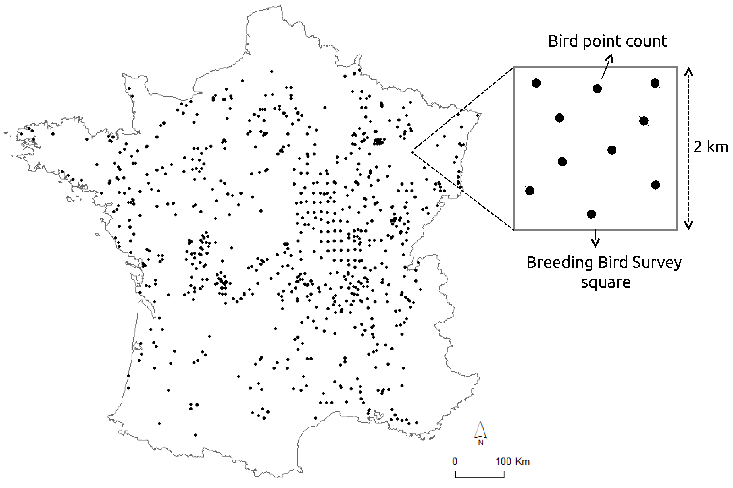
30]. In the FBBS program, each observer provides a point location, and a randomly 2 km × 2 km survey square shaped plot is selected around a radius of 10 km from this location. Each plot contain 10 point counts with 100 m radii which are separated from each other by 300 m at a minimum and scattered in the landscape in order to best represent the diversity of habitats (Figure 1). Each point count is performed twice a year during the breeding season (from April to mid-June) to record early singing species as well as last migrants. In each point count, heard or seen species are recorded during 5 min between 1 h and 4 h after sunrise. In our study, we focused the analyses on the year 2010 for which the sampling effort was high and well distributed at the national scale (a total of 1091 plots). For each point count in the surveyed plot squares, the maximum count over the two visits was retained for each species. We excluded raptors that have home range sizes (several tens of hectares) much higher than point count areas. We also excluded urban and wetland species because their habitats were poorly sampled compared to agricultural and woodland habitats. Moreover, the DHI components based on fPAR is is not available in the heart of the cities.
Plots were filtered according to the quality of the satellite images available on their locations (see 
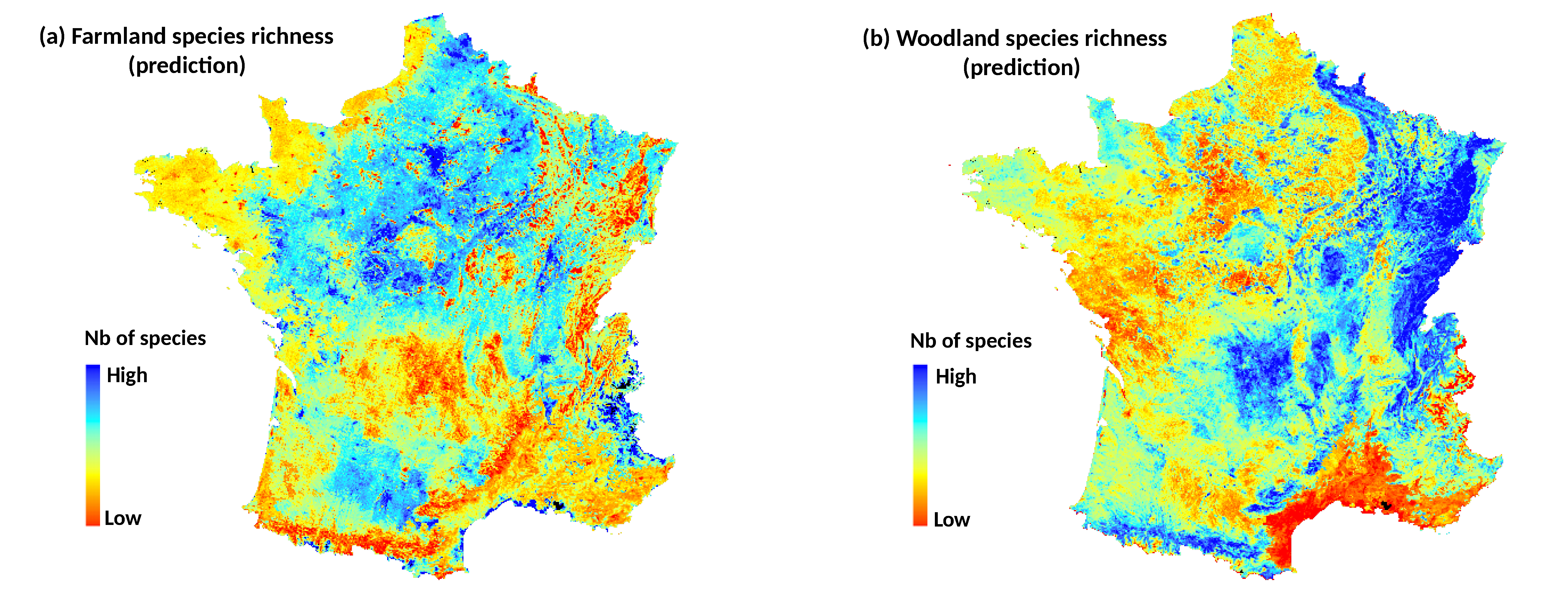
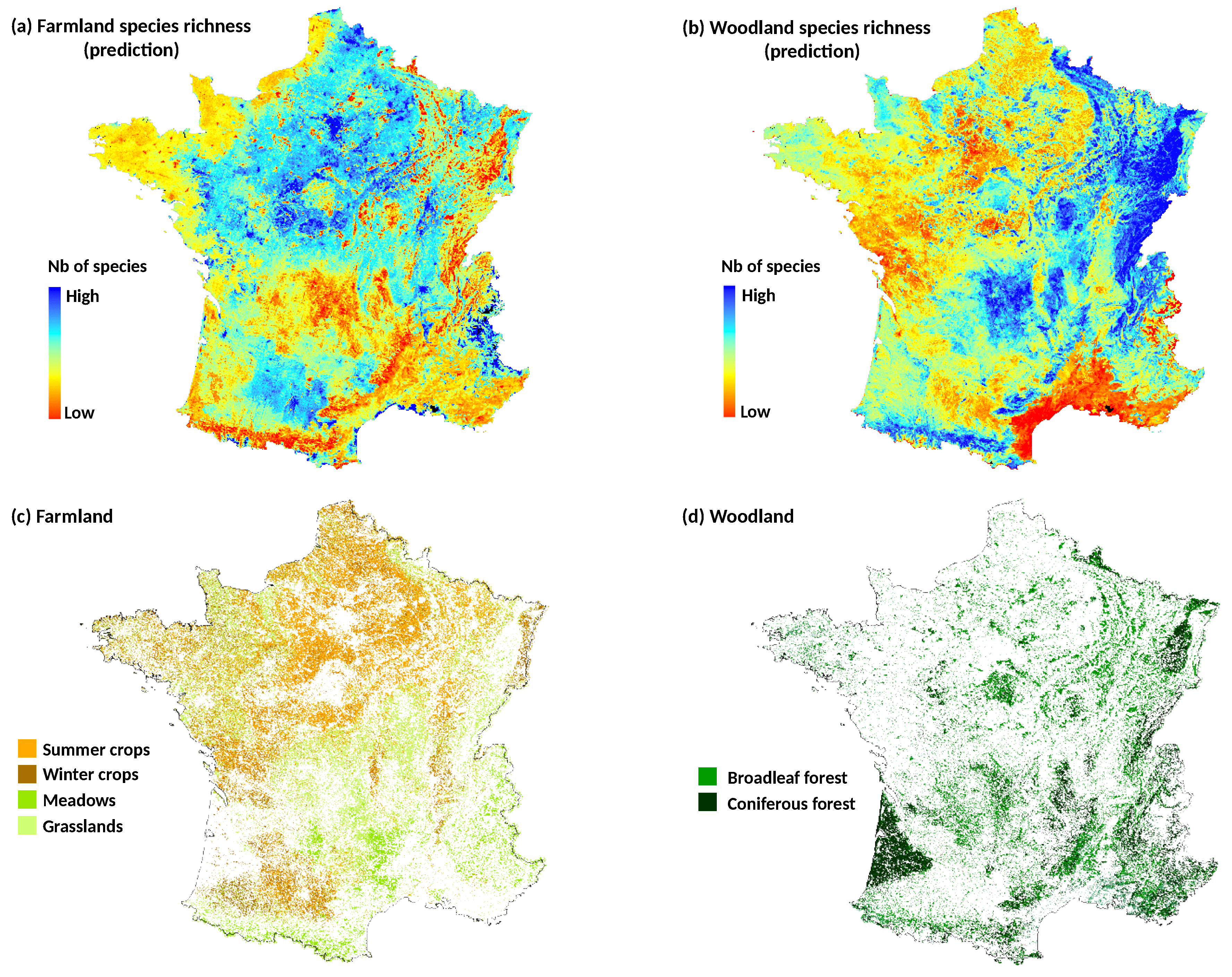
Section 2.2) and 759 plots were finally considered in the analyses. Because birds are expected to respond differently to landscape habitats according to their ecological requirements, four metrics of species richness (SR) per plot square were computed from the species observed at point counts. The first two metrics of SR were related to woodland species and farmland species (specialists of woodland and farmland habitats). The others were related to habitat generalists, and total species richness computed as the sum of all species (see Appendix A for species names). These bird groups (guilds) were based on species information available at the national level (http://vigienature.mnhn.fr).

2.2. Climate and Satellite Data

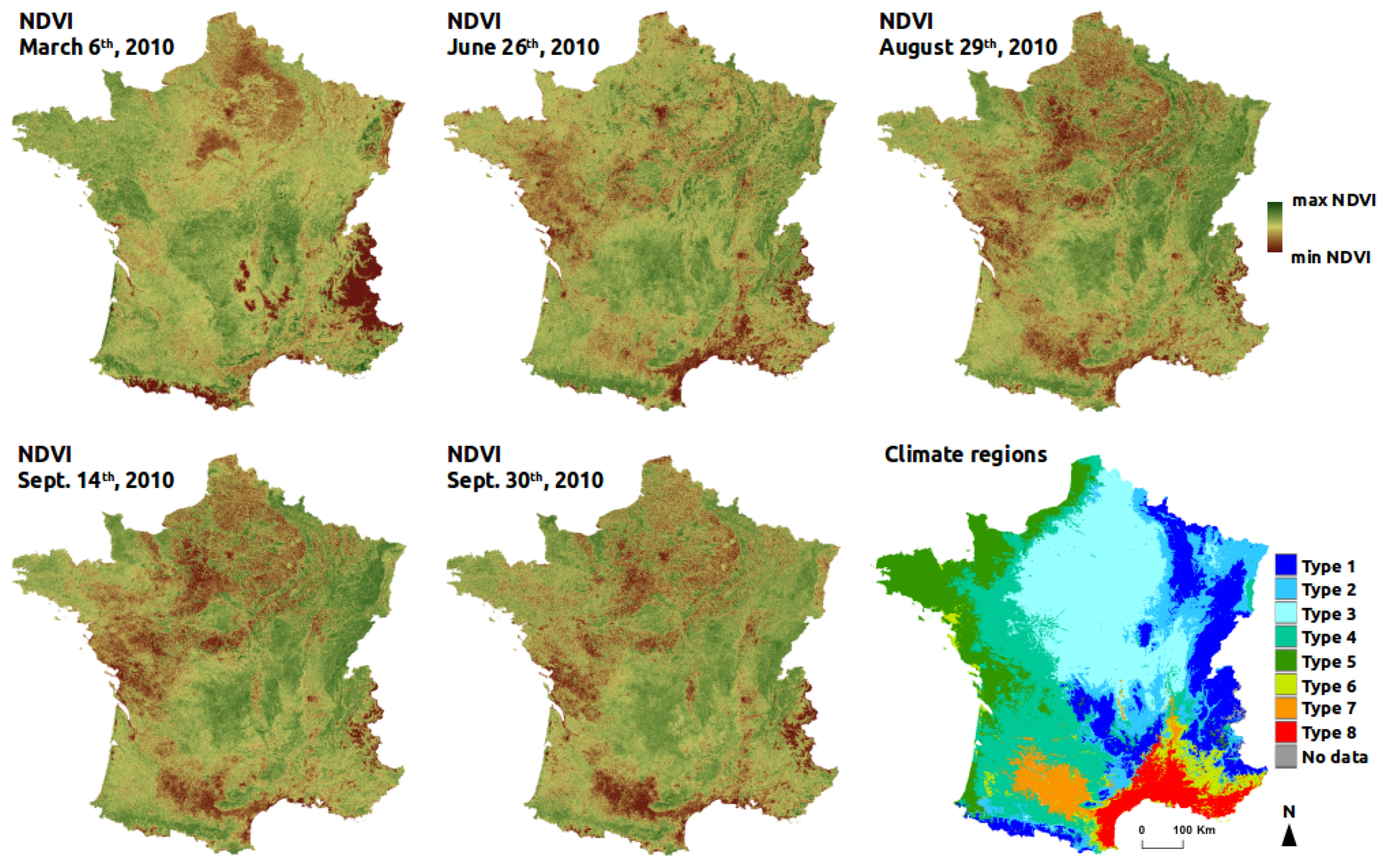
Because avifauna patterns are driven by large climate gradients at the French national scale, a map of macro-climate regions of France was used to derive a climate factor. The delineation of the climate regions in this map is based on 14 temperature and precipitation variables calculated from a 30-year period of climate data (1971–2000) provided by the french national meteorological service [31]. The map is composed of eight regions (Figure 2): the climate of mountain areas (type 1); the semi-continental climate and the climate of peripheral mountain areas (type 2); the degraded oceanic climate of the north and center plains (type 3); the altered oceanic climate (type 4); the marked oceanic climate (type 5); the altered Mediterranean climate (type 6); the southwest basin climate (type 7); and the marked Mediterranean climate (type 8). Based on this map, the dominant climate region was estimated for each plot of bird data and defined as one qualitative predictor. An alternative would have been to use WorldClim2 data which are locally defined at 1 km 2 scale [32]. However, these data are based on an interpolation using fewer weather stations than the map defined by [31] at French scale. This is why we retained the first source of data (i.e., map of macro-climate regions).
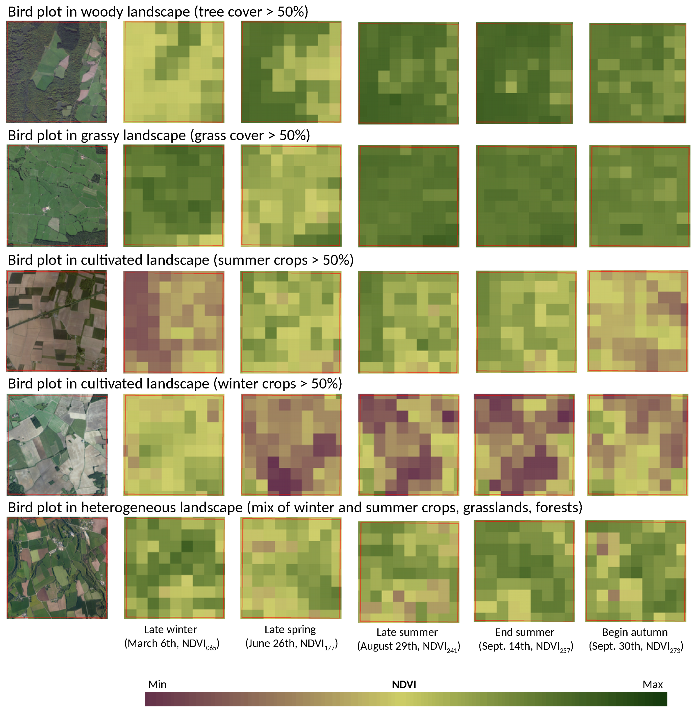
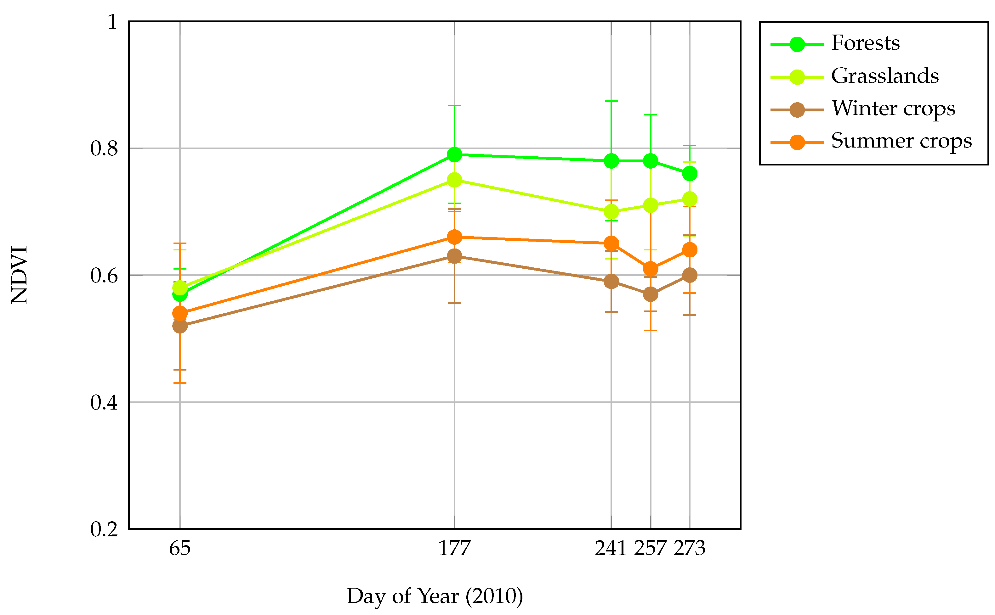
Normalized Difference Vegetation Index (NDVI) was used to provide surrogate of local vegetation cover and landscape heterogeneity patterns over France. The Terra-MODIS NDVI 16-day-composit product at 250-m spatial resolution (MOD13Q1) was retained. To accommodate for seasonal variation and evaluate the temporal effect of NDVI on models performance, five time periods in 2010 were selected (Figure 2): late winter (6 March 2010, NDVI 065 ), before leaves growing of deciduous tree; late spring (26 June 2010, NDVI 177 ), before winter crops harvesting; late summer (29 August 2010, NDVI 241 ), after winter crops harvesting before summer crops harvesting; end summer (14 September 2010, NDVI 257 ), after partial summer crops harvesting; begin autumn (30 September 2010, NDVI 273 ), after full crops harvesting. At these time periods, landscape composition and heterogeneity are revealed differently in NDVI data. In winter, NDVI values are low in the deciduous forests and in the non-cultivated agricultural parcels because of absence of photosynthetic activity. In spring and summer, NDVI reaches its highest values, mainly in winter and summer crops respectively, but also in grasslands and forests. In autumn, after all crops harvesting, NDVI discriminates well forests and open habitats because of higher difference of NDVI values, agricultural parcels being bare (see Appendix E).
The NDVI data of each time period were selected after checking the MODIS quality layers of all the 16-day time series products of 2010. Based on the average value of the MOD13Q1 pixel reliability over France (0 = good, 1 = marginal data, 2 = snow/ice, 3 = cloudy), the images showing the highest quality (i.e., having the lowest average quality index) were retained for each time period. Then, a filter was applied on the bird survey plots available ( n = 1091 ). Plots including NDVI pixels of bad quality were removed. Only plots composed of 100% of good pixels (i.e., with a pixel reliability = 0) at the five time periods were used ( n = 759 ). Finally, NDVI values in these plots were summarized through several statistical predictors: minimum, maximum, range, average, median, and standard deviation. In order to prevent multicollinearity between covariates, only the average (Avg) and standard deviation (SD) predictors were retained (Spearman’s |Rho| < 0.7 ) [33]. The average predictor is a proxy of landscape productivity and the dominant land cover in the plot. The standard deviation reflects landscape heterogeneity.
To examine whether seasonal variations effect of NDVI on the models performance depends on the landscape context, we used land cover/land use datasets to calculate landscape composition in each bird plot. The forest layer was obtained from a nationwide highly detailed vector spatial database (BDTopo®, French mapping agency IGN) at 1-m resolution. For agricultural areas, the graphic parcel register (RPG) of 2010 was used. The French RPG database is produced annually since 2002 in application of the EU directives related to the Common Agricultural Policy. The land use information, based on a 28 class nomenclature (including several types of crops, as well as artificial and natural grasslands), is obtained from the farmers’ declaration of their cultivated areas. The information is defined at the agricultural block level composed of one single field or several contiguous ones. For each block, the proportion of each crop type is provided but without the spatial distribution of crops within the block.
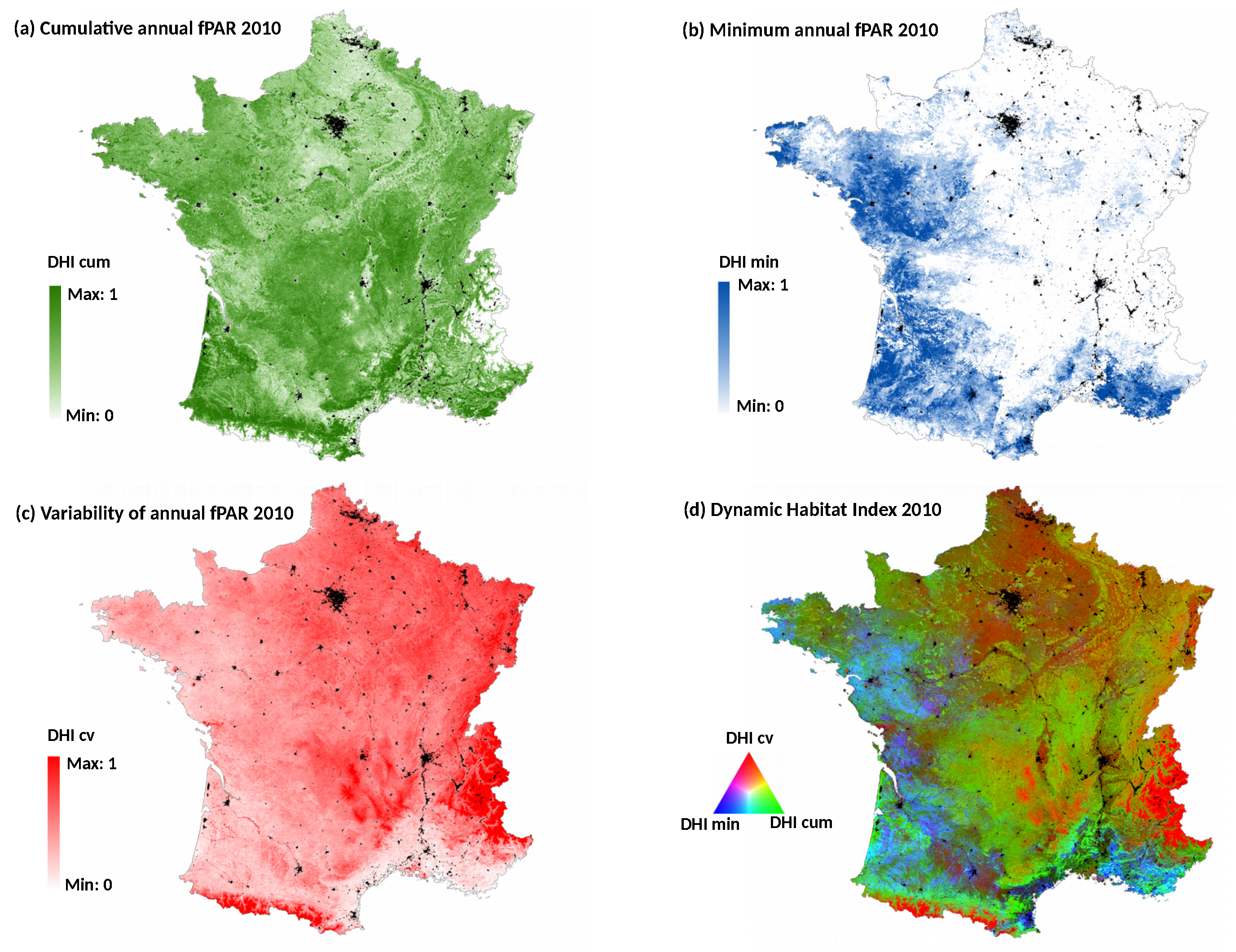
The Dynamic Habitat Index of 2010 was also calculated at the national scale, in order to compare the performance of the DHI-based model with the ones based on single date NDVI. The DHI was derived from the most detailed MODIS fPAR (fraction of Photosynthetically Active Radiation) 8-day composite product at 500-m spatial resolution (MOD15A2H) [34]. It includes three components [26]: (1) the cumulative annual fPAR (DHI cum) reflecting the overall potential of vegetation productivity; (2) the minimum annual fPAR value (DHI min) indicating the minimum amount of vegetated cover; and (3) the coefficient of variation of annual fPAR (DHI cv) expressing the seasonality in productivity (Figure 3). The average and standard deviation of the three DHI components were calculated for each plot of bird data ( n = 759 ) and used as dependent variables. All the variables were retained in the bird-habitat models after checking correlations between them (Spearman’s |Rho| < 0.7 ). In order to avoid bias in the comparison with NDVI-based models because of difference in spatial resolution, NDVI variables were also computed from the MODIS product at 500-m (MOD13A1). To evaluate the seasonal effect of NDVI on models’s performance independently of DHI (see above), we kept the most detailed NDVI data at 250-m. This spatial resolution is likely to produce models with higher explanatory and predictive performances [21].

2.3. Statistical Analysis

In a first time, we built models at national scale using the total filtered bird dataset ( n = 759 ). We compared explanatory and predictive performances of NDVI data at several time periods with DHI data. For each of the four species richness metrics, we first constructed a model with only the climate variable, i.e., the dominant climate region of the bird plot, as predictor (e.g., SR w o o d l a n d ~Climate). Then, we added into the climate model both NDVI variables (Avg and SD) of each time period in five separate models (e.g., SR w o o d l a n d ~Climate + Avg.NDVI 065 + SD.NDVI 065 ). Finally, we fitted a final model including DHI variables (6 predictors related to the Avg and SD of the three DHI components, see above) and the climate predictor.
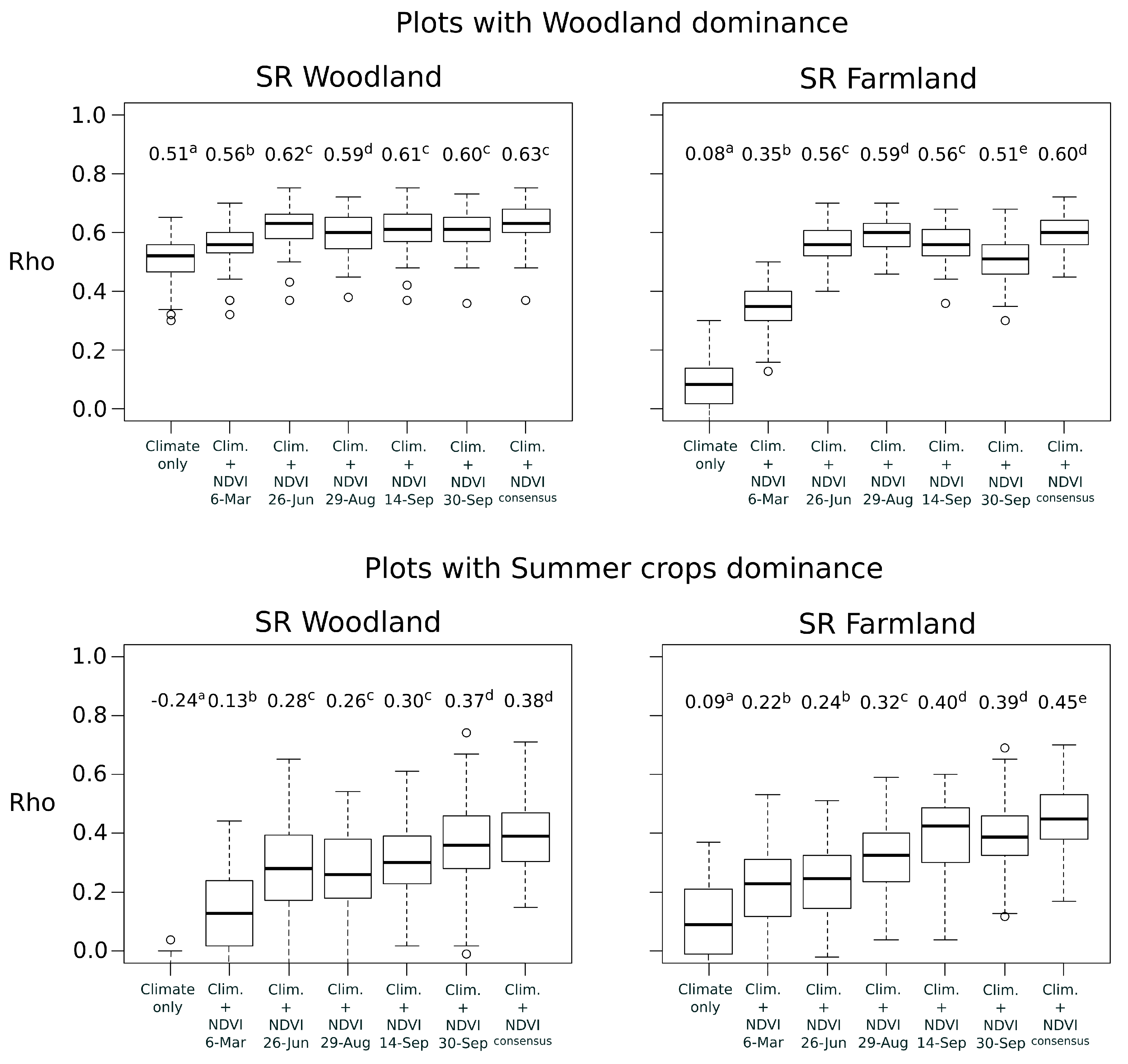
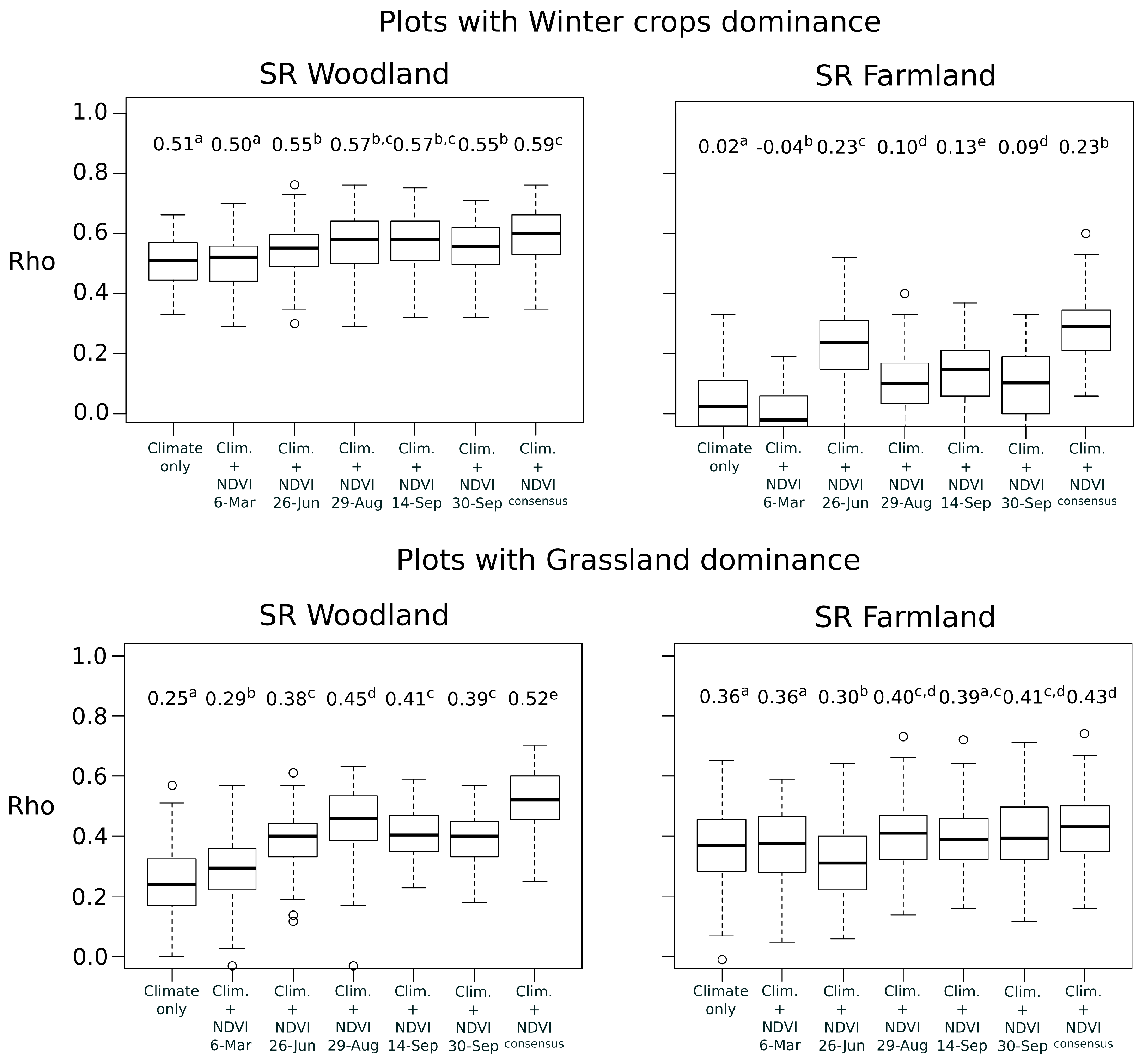
In a second time, we examined whether the best time period of NDVI depended on the plot land cover context. This analysis was only applied to woodland and farmland species richness that were the best explained bird metrics at national scale. We partitioned bird national data into subsets, according to the dominant land cover of the bird plot squares. Landscape composition in each plot was calculated as the proportion of area occupied by four land covers: woody vegetation (including hedgerows), permanent grasslands, winter crops (mainly wheat and barley) and summer crops (mainly maize and sunflower). Because agricultural blocks of the land cover map (RPG) may cover partially the bird plot squares, only the blocks included by at least 70% in the plots were conserved for the estimation. Based on the land cover proportions, four subsets of bird plots were defined with the constraint to obtain a sample size large enough (i.e., with n > 100 ) and a high dominance of a specific land cover (Table 1). For each subset, we built models with climate and NDVI variables of each date as for the national scale.
Relationships between bird species richness and predictors were explored using generalized additive models (GAMs) with R version 3.1.0 software [35] and the gam package [36]. The general expression of GAM model is [37]:
g ( E ( Y | X 1 , X 2 , , X p ) ) = f 0 + f 1 ( X 1 ) + f 2 ( X 2 ) + + f p ( X p ) = f 0 + i = 1 p f i ( X i )
where Y is the response variable, X i the predictors, f i the non-parametric smooth functions and g the link function relating to the expected value of Y.
GAMs present the advantage to consider non-linear effects between response and predictor variables. Poisson distribution and a log link function were used to calibrate the models. The most parsimonious models (i.e., with the lowest Akaike Information Criterion values) were selected by stepwise backward and forward variable selection [38]. In addition, the procedure was allowed to select from one to four degrees of smoothing (1 = no smoothing) for each quantitative variable in GAMs.
The goodness of fit of the models (explanatory performance) was quantified by the amount of explained deviance (% D 2 ). The independent contribution of each variable to explain species richness was also estimated from a hierarchical partitioning procedure [39].
The predictive performance was calculated by k-fold cross-validation [40]. The initial dataset was splitted randomly in three groups of equal size ( k = 3 ). Two groups were used to calibrate the model and the third group was used as a test set to evaluate predictions. The concordance between predictions and observations was measured with the Spearman rank correlations (Rho) ranging from 1 to +1 [41]. The correlation is considered to be weak for 1 < Rho < 0.25, fair for 0.25 < Rho < 0.50, moderate for 0.50 < Rho < 0.75 and strong for Rho > 0.75 [42]. Cross-validation was repeated 100 times per model to obtain a variance of Rho. The predictive performances between the models were compared using Wilcoxon rank-sum non-parametric tests.
In order to assess whether the combination of multiple NDVI time periods lead to higher predictive performances than the use of a single date, a consensus approach was also followed. Because NDVI variables of different time periods were often highly correlated (Rho > 0.70) they could not be included simultaneously into a single model [33]. Alternatively, the consensus approach provides means to combine ensembles of model predictions, and to test if the predictive performance is higher after combination. This approach is usually adopted in species distribution modelling to combine outputs of single modelling techniques and to reduce uncertainty of predictions [43]. Here, the outputs of single-date models were combined with the Weighted Average (WA) consensus method [43]. The predictions were calculated as the mean of predictions of single-date models weighted by their individual predictive performance (mean Rho). The concordance between predictions and observations was evaluated in the same way than the models based on single date.
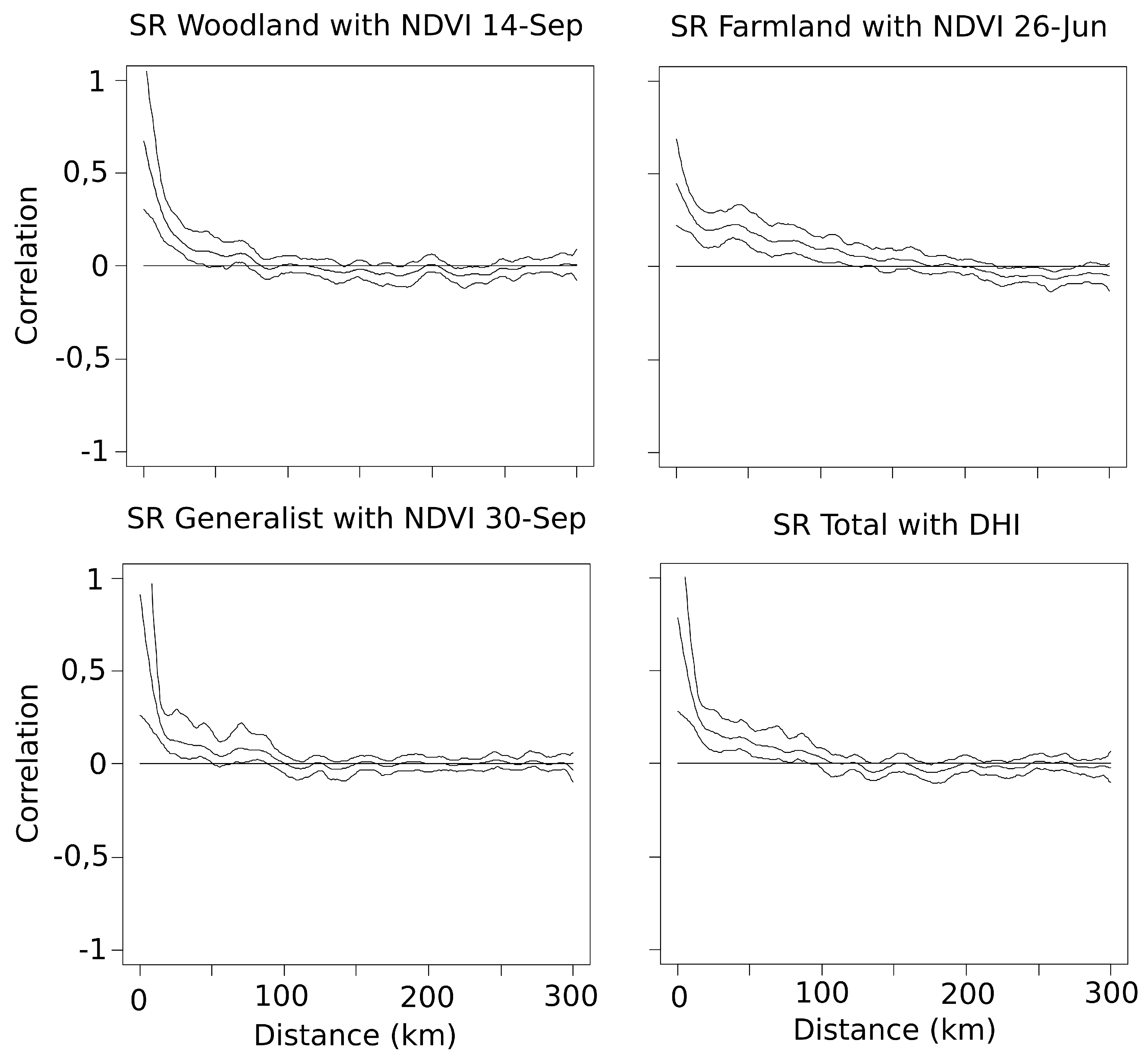
Spatial autocorrelation of residuals was tested for each best model by computing non parametric spline correlograms using the ncf package version 1.1-3 for R [44]. Neighbours were considered until a distance of 300 km. Because a positive inherent autocorrelation was observed only for the very close surveyed plot squares (Spatial autocorrelation < 0.2 within 20 km; average distance of the closest square = 8.15 ± 7.01 km; Appendix B), we considered the potential effect as not significant in the analysis [45].

3. Results

3.1. Comparison of Single-Date NDVI Models with DHI According to Species Richness Metrics

Bird-habitat models showed different explanatory performances according to the species richness metrics, data types and acquisition periods considered (Table 2). Whatever the time period of NDVI, climate always had a significant effect on the four species richness metrics. For the models based on climate only, the explanatory power is high for woodland species ( D 2 = 23 %) but more limited for the other groups, with the lowest explanatory power for farmland species ( D 2 = 6 %). Adding NDVI or DHI variables to climate increased the performance of the models. The best fits were observed for woodland ( D 2 = 45 % at 250 m) and farmland ( D 2 = 35 % at 250 m) birds. The lowest values were found for generalist species (from D 2 = 7 % to D 2 = 14 % at 250 m). The DHI-based models showed similar performances in comparison with the best NDVI-based models for woodland birds ( D 2 = 43 %), generalist species ( D 2 = 13 %) and total species richness ( D 2 = 20 %). By contrast, the explanatory power was lower for farmland species ( D 2 = 21 %). The same conclusions between the DHI and NDVI-based models were obtained whatever the spatial resolution of NDVI.
Regarding NDVI variables, average NDVI was more important than standard-deviation NDVI for explaining species richness metrics. For DHI, average DHI cv (i.e., seasonality, based on the coefficient of variation of annual fPAR) and average DHI cum (i.e., productivity, based on the cumulative annual fPAR) contributed most (see Appendix C).
Considering the effect of NDVI seasonal variation on the model performances, whatever the landscape context, late winter (NDVI 6-Mar) was the least accurate time period for every species richness variable. The optimal NDVI time period varied according to the bird species richness metric (Table 2). For woodland species richness, end summer (NDVI 14-Sep) was the best time period, but only slight difference in accuracy was observed with the other periods, except for winter (NDVI 6-Mar). For farmland species richness, late spring (NDVI 26-Jun) was the most adapted. For generalist and total species richness, several periods were similarly accurate. The seasonal variation of NDVI was a lower impact on these response variables since the contribution of NDVI was limited (Appendix C).
The response shapes to the NDVI variables were different according to the bird group considered (Figure 4). For woodland birds, species richness increased continuously with the average NDVI variable. By contrast, farmland species richness was quite stable for low values of average NDVI but decreased when average NDVI reached 0.7. Total richness increased until the same threshold (average NDVI of 0.7) and decreased after this value. The curves were constructed after selecting the best NDVI time period for each bird group.
In terms of predictive performance, the best predictions were obtained for woodland and farmland birds (maximum mean Rho = 0.70 and 0.53, respectively) (Figure 5). Generalist and total species richness showed fairly good but lower predictive accuracies (maximum mean Rho = 0.36 and Rho = 0.39, respectively). Comparing to the single-date models, the consensus NDVI approach showed superior predictive performances only for generalist species richness. The predictive accuracy of DHI was slightly but significantly lower than the best NDVI single-date model for all the bird groups.
The national spatial distributions of woodland and farmland species richness were predicted using their respective best model, showing a consistent pattern over France. Where the farmland bird species richness is high, the richness is low for woodland birds (Figure 6). In terms of absolute value, caution must be taken because of projection uncertainty in some areas (limited bird plots in mountain and Mediterranean regions used for model calibrations) [46].

3.2. Comparison of NDVI Single-Date Models According to the Land Cover Context

The effect of seasonal changes of NDVI on models performance depends on the bird community but is also modulated by the dominant landscape composition existing in the bird plots. In other words, for the same group of birds, the best NDVI acquisition date may vary according to the dominant land cover. This effect was evaluated for woodland and farmland birds only.
In forested landscapes, with plots dominated by woody vegetation, late winter (NDVI 6-Mar) was the least accurate time period to explain woodland species richness ( Δ D 2 = 5 % in comparison to the best date; Table 3). The other periods fitted better with close explanatory power. For farmland species richness, late spring (NDVI 26-Jun) or late summer (NDVI 29-Aug) were the most appropriated.
In agricultural landscapes, with plots dominated by winter crops or summer crops, end summer (NDVI 14-Sep) and begin of autumn (NDVI 30-Sep) explained better farmland and woodland species richness respectively (Table 3).
In grassy landscapes, with plots dominated by permanent grasslands, late summer (NDVI 29-Aug) fitted better for woodland birds. For farmland birds, begin of autumn (NDVI 30-Sep) remained the most adapted.
In a general way, landscape composition in the bird plot had an impact on the best NDVI time period for explaining woodland and farmland birds. However, end summer (NDVI 14-Sep) and begin of autumn (NDVI 30-Sep) appeared to be the most appropriate in majority (Table 3).
Predictive accuracies showed close results with explanatory performances (Figure 7). Difference appeared only for farmland birds in agricultural landscapes composed of winter crops but Rho values were generally low for this case. Comparing to the single-date models, the consensus approach enabled to improve the predictions significantly for only two cases (SR woodland in grassy landscapes and SR farmland in agricultural landscapes with summer crops) (Figure 7).

4. Discussion

4.1. Single-Date NDVI Is as Accurate as DHI or Multi-Date NDVI to Explain and Predict Bird Species Richness

Our study is the first to evaluate the potential added value of DHI components, compared to NDVI, to model the relationships between bird community and landscape structure. The results suggest that the integrative DHI components which summarizes vegetation productivity and heterogeneity over the year are not the best predictors to explain and predict diversity patterns of breeding birds over France. We found very close performances between NDVI and DHI-based models for woodland birds, generalists and total species richness. However, we observed that single-date NDVI models fitted and predicted better than DHI model for farmland birds (with a difference around 14% for the explained deviance). This is true whatever the spatial resolution of the NDVI product. NDVI at 500-m was highly correlated with NDVI at 250-m (r > 0.92 between average NDVI variables for all dates). Contrary to our assumption [21], difference in spatial resolution had no effect on models’ performance. At the scale of analysis (bird plot of 4 km 2 ), average and standard deviation of NDVI 250-m and NDVI 500-m are similar.
A possible explanation of the non-superiority of the DHI could be the difference in proxies of vegetation productivity. The DHI is based on the fPAR (derived from a physically based model) and not on NDVI which may saturate at high biomass. But a recent study showed that DHI derived from vegetation index (such as NDVI or EVI) was weaker to explain bird species richness than DHI computed from MODIS fPAR, LAI or Gross Primary Productivity (GPP) [29].
Previous studies testing the predictive power of DHI on bird species diversity were based on very large sample units such as USA ecoregions (around 90,000 km 2 in average) that are homogeneous in terms of environmental conditions [29,48]. Compared to our analysis, similar degrees of correlation were observed at this spatial extent with variations depending on avian functional groups. In [29], the multiple regression model predicted species richness of woodland birds using the fPAR-derived DHI with an adjusted coefficient of determination ( % R a d j 2 ) equals to 0.58. In [48] the explained variance was weaker ( % R a d j 2 = 0.37 ). In both cases, cumulative DHI was most predictive which can be referred to the species-energy theory [49]. In our study, the sample unit of investigation is substantially smaller (4 km 2 ) and match with the bird survey. At this fine scale, birds mainly respond to local landscape factors such as resource availability, habitat amount and habitat diversity [50]. The results show that DHI discriminates the habitat composition and heterogeneity less accurately at this scale than an appropriate single-date NDVI. This is especially true in agricultural landscapes where differences in DHI between crops, grasslands and woodlands may be less pronounced than NDVI at best date because of the integrated greeness over the year. Therefore, the average and standard deviation NDVI variables (proxies of dominant habitat identity and spatial heterogeneity) explain more bird community variance than cumulative and variation DHI (proxies of annual productivity and seasonnality). This finding is confirmed by the fact that the consensus approach that combine multiple time periods of NDVI has no real effect on models performance. This is also in line with previous works which demonstrated that NDVI-based measure of seasonal vegetation productivity is a stronger predictor than annual NDVI [17,51].

4.2. Best Single-Date NDVI Is Not Synchronous with the Acquisition Time Period of Bird Data

In most ecological studies, it is usual to make the acquisition date of images consistent with the ground observations in order to avoid misinterpretations [14,17,52,53]. However, as showed by the results of this study, when NDVI is used as proxy to estimate species diversity at fine scale, this common sens rule must be revised since NDVI is time-dependent.
This observation supports the conclusions of a previous study carried out in a small area of southwestern France [21]. The best NDVI time period to predict bird diversity patterns at the survey level is the one that enable to separate the mixture of crops, open grasslands and ligneous habitats. These components explain bird requirements for breeding and foraging according to functional groups. Depending on the season, differences between habitats are more or less apparent in the NDVI images (Figure 8). Because NDVI in winter has lower values in deciduous forests, this time period leads to underestimate woodland species richness. For other seasons, models performance is equivalent. For farmland species, overestimation appears for time periods where semi-natural habitats are confused with crops because of close values of NDVI. This is the case for winter and summer crops before senescence or harvesting (at the end of june and august, varying by the location). After soil tillage, cultivated areas and other habitats are better discriminated.
Until now, this time effect has paid little attention in species distribution models based on continuous remotely sensed variables. Several studies evaluated if seasonal bird richness (breeding vs. wintering) was linked to change in productivity during the year [17,53] but few of them analyzed the optimal matching between the seasonal NDVI and the bird survey although asynchrony was already observed [22,52]. This is probably due to the macro ecological hypothesis that underpins these studies and which supposes that productivity determines species richness [54]. In our case, average NDVI reflects dominant habitat identity in each plot and this dominance is best displayed in late spring or begin of autumn. This variable was especially relevant for explaining woodland species richness and farmland species richness (Appendix D). Woodland species richness, which is mainly composed of tree-nesting species feeding on invertebrates (e.g., Certia brachydactyla, Erithacus rubecula, Sitta europea) increased constantly with NDVI. Farmland species richness was constant until a NDVI value of 0.7 and then decreased. The lowest values of NDVI correspond to the most open landscapes (Appendix E) that facilitate farmland ground-nesting species avoiding high vegetation structures (e.g., Alauda arvensis, Alectoris rufa, Coturnix coturnix). Intermediate values of NDVI represent heterogeneous landscapes with grasslands and hedgerows that favor farmland species nesting in hedgerows and requiring complementation of habitats (e.g., Carduelis cannabina, Emberiza cirlus, Emberiza citrinella) [6]. Landscape heterogeneity, through standard deviation NDVI, also explained a part of the species richness of the two bird groups but to a lesser extent. Heterogeneity may increase differentiation of ecological niches allowing different species to coexist in a same landscape [14,55,56]. However, the effects of heterogeneity are related to the degree of habitat specialization for the species. Highly specialized bird species tend to be negatively affected by landscape heterogeneity [57]. A more refined discrimination between bird species of each community, according to their habitat specialization, may have led to different conclusions [58].

4.3. Best Single-Date NDVI Is Context-Dependent, Varying According to the Dominant Land Use

Our results showed that best single-date NDVI for modeling bird distribution patterns is time-dependent but is also modulated by the landscape context of the bird plots. In landscapes dominated by winter crops or summer crops, we found that end summer (14 September ) and begin of autumn (30 September) were the best periods to explain farmland and woodland bird species richness over France. For other seasons, crop cover with high NDVI values affect negatively the estimation of the species richness (leading to an under or overestimation depending on the bird group considered). In landscapes dominated by grasslands, late spring (26 June) and late summer (29 August) were the most adequate periods for SR woodland. This is also the case in woody landscape to explain SR farmland. These time periods match with the peak of woodland and grassland vegetation productivity leading to better accurate estimations.
Because the proportion of the dominant land use in the surveyed square was sometimes low in the analysis (although a majority proportion was ensured in bird plots), a deeper analysis should be further developed to confirm the results, using a most exhaustive dataset.

4.4. Adding Habitat to Climate Variables Improve Predictions of Local Bird Patterns at National Scale

We observed that adding NDVI or DHI data reflecting local habitats in bioclimatic models greatly improve the performances of species richness estimations. The utility of habitat variables was particularly important for woodland and farmland specialists, and much less for generalist species whose individuals can find their resources in a wide range of habitats. This result is in line with previous studies showing the role of climate as driver of bird species distribution at macro-scale, combined with land cover at finer spatial resolutions [59,60]. However, the role of climate as causal determinant of species’ geographic distributions is still in debate [61,62]. Positive correlation with climate could appeared for non-climatic reasons, due to the existence of spatially structured processes which are themselves not necessary related to coarse environmental variables [63]. At fine resolution, landscape and habitat composition which is highly variable between plots effectively increases the performance of species richness models. NDVI data can thus be of great value for building bird models, especially for specialist species whose populations decline drastically [64].

5. Conclusions

As confirmed in this study, continuous (unclassified) predictors derived from satellite imagery contribute to build efficient SDM at large spatial scale [7]. However, because of temporal variability of remotely sensed predictors over the year, acquisition time periods of the data affect the models’ performance. Here, we found that:
  • Compared to a combination of multiple NDVI time periods or to the components of DHI, performance of bird models is higher with single time period of NDVI variables.
  • Models’ performance is time and context-dependent. At the French scale, end summer (NDVI 14-Sep) and begin of autumn (NDVI 30-Sep) are in most cases, the best time periods to explain and predict woodland and farmland birds species richness.
  • Best time period of NDVI is the one that better reflect dominant habitats in the bird survey plots.
  • Habitat components at finer scale have to be combined with climate variables at macro scale to explain and predict patterns of habitat specialist species.
These findings suggest that the most powerful approach is the simplest one. Only one image of appropriate time period is required for mapping bird species richness. This makes the use of unclassified remotely sensed data very operational for bird monitoring programs. Further work is needed to confirm the conclusions from multiple years and to verify the stability of the relationships. Predictions could also be improved using the new Sentinel-2 time series of higher spatial resolution.

Author Contributions

S.B. and D.S. conceived and designed the experiments; D.S., S.L. and P.-A.H. prepared the image data; S.B. and S.L. prepared the bird data; S.B, D.S. and S.L. performed the experiments and analyzed the results; S.B. and D.S. wrote the paper with feedback from P.-A.H. and S.L.

Funding

This research was partially funded by Institut National de la Recherche Agronomique (Payote research group) through the S. Lefèvre’s internship funding.

Acknowledgments

We greatly thank to Frédéric Jiguet (MNHN) and Christophe Sausse (Terres Inovia) for allowing access to the French breeding bird data (STOC EPS program) and all the volunteer ornithologists who make the FBBS possible.

Conflicts of Interest

The authors declare no conflict of interest.

Appendix A. Common Bird Species Selected in the Study

Table A1. Species composition of the four bird groups according to the French Breeding Bird Survey classification.
Latin NamesSR WoodlandSR FarmlandSR GeneralistSR Total
Alauda arvensis X X
Alectoris rufa X X
Anthus campestris X X
Anthus pratensis X X
Carduelis cannabina X X
Certhia brachydactylaX X
Certhia familiarisX X
Coccothraustes coccothraustesX X
Columba palumbus XX
Coturnix coturnix X X
Cuculus canorus XX
Dendrocopos majorX X
Dendrocopos mediusX X
Dryocopus martiusX X
Emberiza calendra X X
Emberiza cirlus X X
Emberiza citrinella X X
Emberiza hortulana X X
Erithacus rubeculaX X
Fringilla coelebs XX
Galerida cristata X X
Garrulus glandarius XX
Hyppolais polyglotta XX
Lanius collurio X X
Lullula arborea X X
Luscinia megarhinchos XX
Motacilla flava X X
Oenanthe oenanthe X X
Oriolus oriolus XX
Parus aterX X
Parus caeruleus XX
Parus cristatusX X
Parus major XX
Parus palustrisXX X
Perdix perdix X X
Phylloscopus bonelliX X
Phylloscopus collybitaX X
Phylloscopus sibilatrixX X
Phylloscopus trochilusX X
Picus canusX X
Picus viridis XX
Prunella modularis XX
Pyrrhula pyrrhulaX X
Regulus ignicapillaX X
Regulus regulusX X
Saxicola rubetra X X
Saxicola torquata X X
Sitta europeaX X
Streptopelia turturX X
Sylvia atricapilla XX
Sylvia communis X X
Sylvia melanocephalaX X
Troglodytes troglodytesX X
Turdus merula XX
Turdus philomelosX X
Turdus viscivorusX X
Upupa epops X X

Appendix B. Spatial Autocorrelation

Figure A1. Non parametric spline correlograms, with 95% pointwise bootstrap confidence intervals of the Pearson residuals from GAMs, based on the best model of each bird group.
Remotesensing 10 01136 g0a1

Appendix C. Contribution of Each Explanatory Variable in the Bird-Habitat Models

Table A2. Relative importance of each variable (in %) for explaining species richness (SR) of the four groups of birds at each date of NDVI at 250-m spatial resolution. This analysis was based on hierachical partitioning procedures using the whole bird dataset ( n = 759 ) and the NDVI-based remotely sensed variables with climate.
NDVI 6-MarNDVI 26-JunNDVI 29-AugNDVI 14-SepNDVI 30-Sep
SR Woodland
Climate7732333333
Average NDVI1360585854
Stand. dev. NDVI1089913
SR Farmland
Climate7836292933
Average NDVI750514948
Stand. dev. NDVI1514202219
SR Generalist
Climate7294999486
Average NDVI2711411
Stand. dev. NDVI15023
SR Total
Climate8379777371
Average NDVI1419202326
Stand. dev. NDVI31343
Table A3. Relative importance of each variable (in %) for explaining species richness (SR) of the four groups of birds. This analysis was based on hierachical partitioning procedures using the whole bird dataset ( n = 759 ) and the DHI-based remotely sensed variables with climate.
SR WoodlandSR FarmlandSR GeneralistSR Total
Climate26386551
Average DHI min64514
Stand. dev. DHI min3147
Average DHI cum2836810
Stand. dev. DHI cum1122
Average DHI cv34201614
Stand. dev. DHI cv2002

Appendix D. NDVI Effect in the Best Models

Table A4. Signs of NDVI predictors (average and standard deviation) for each bird species richness (SR) related to models calibrated with the best time period. NS indicates that the predictor was not included in the best model after variable selection.
Avg NDVISD NDVI
SR Woodland++
SR Farmland+
SR Generalist+NS
SR Total+NS

Appendix E. Seasonal Variation of NDVI According to the Dominant Land Cover

Figure A2. NDVI temporal profiles (average value ± standard deviation) for bird plots dominated by forests, grasslands, winter crops and summer crops.
Remotesensing 10 01136 g0a2

References

  1. Hitch, A.T.; Leberg, P.L. Breeding distributions of North American bird species moving north as a result of climate change. Conserv. Biol. 2007, 21, 534–539. [Google Scholar] [CrossRef] [PubMed]
  2. Barbet-Massin, M.; Jetz, W. A 40-year, continent-wide, multispecies assessment of relevant climate predictors for species distribution modelling. Divers. Distrib. 2014, 20, 1285–1295. [Google Scholar] [CrossRef]
  3. Gillings, S.; Balmer, D.E.; Fuller, R.J. Directionality of recent bird distribution shifts and climate change in Great Britain. Glob. Chang. Biol. 2015, 21, 2155–2168. [Google Scholar] [CrossRef] [PubMed]
  4. Thuiller, W.; Araújo, M.B.; Lavorel, S. Do we need land-cover data to model species distributions in Europe? J. Biogeogr. 2004, 31, 353–361. [Google Scholar] [CrossRef]
  5. Heikkinen, R.K.; Luoto, M.; Virkkala, R.; Rainio, K. Effects of habitat cover, landscape structure and spatial variables on the abundance of birds in an agricultural–forest mosaic. J. Appl. Ecol. 2004, 41, 824–835. [Google Scholar] [CrossRef]
  6. Bonthoux, S.; Balent, G.; Augiron, S.; Baudry, J.; Bretagnolle, V. Geographical generality of bird-habitat relationships depends on species traits. Divers. Distrib. 2017, 23, 1343–1352. [Google Scholar] [CrossRef]
  7. He, K.S.; Bradley, B.A.; Cord, A.F.; Rocchini, D.; Tuanmu, M.N.; Schmidtlein, S.; Turner, W.; Wegmann, M.; Pettorelli, N. Will remote sensing shape the next generation of species distribution models? Remote Sens. Ecol. Conserv. 2015, 1, 4–18. [Google Scholar] [CrossRef]
  8. Gottschalk, T.; Huettmann, F.; Ehlers, M. Thirty years of analysing and modelling avian habitat relationships using satellite imagery data: A review. Int. J. Remote Sens. 2005, 26, 2631–2656. [Google Scholar] [CrossRef]
  9. Price, B.; McAlpine, C.A.; Kutt, A.S.; Phinn, S.R.; Pullar, D.V.; Ludwig, J.A. Continuum or discrete patch landscape models for savanna birds? Towards a pluralistic approach. Ecography 2009, 32, 745–756. [Google Scholar] [CrossRef]
  10. Culbert, P.D.; Radeloff, V.C.; St-Louis, V.; Flather, C.H.; Rittenhouse, C.D.; Albright, T.P.; Pidgeon, A.M. Modeling broad-scale patterns of avian species richness across the Midwestern United States with measures of satellite image texture. Remote Sens. Environ. 2012, 118, 140–150. [Google Scholar] [CrossRef]
  11. Tuanmu, M.N.; Jetz, W. A global, remote sensing-based characterization of terrestrial habitat heterogeneity for biodiversity and ecosystem modelling. Glob. Ecol. Biogeogr. 2015, 24, 1329–1339. [Google Scholar] [CrossRef]
  12. Lausch, A.; Blaschke, T.; Haase, D.; Herzog, F.; Syrbe, R.; Tischendorf, L.; Walz, U. Understanding and quantifying landscape structure—A review on relevant process characteristics, data models and landscape metrics. Ecol. Model. 2015, 295, 31–41. [Google Scholar] [CrossRef]
  13. Cord, A.F.; Klein, D.; Mora, F.; Dech, S. Comparing the suitability of classified land cover data and remote sensing variables for modeling distribution patterns of plants. Ecol. Model. 2014, 272, 129–140. [Google Scholar] [CrossRef]
  14. Duro, D.C.; Girard, J.; King, D.J.; Fahrig, L.; Mitchell, S.; Lindsay, K.; Tischendorf, L. Predicting species diversity in agricultural environments using Landsat TM imagery. Remote Sens. Environ. 2014, 144, 214–225. [Google Scholar] [CrossRef]
  15. Rhodes, C.J.; Henrys, P.; Siriwardena, G.M.; Whittingham, M.J.; Norton, L.R. The relative value of field survey and remote sensing for biodiversity assessment. Methods Ecol. Evol. 2015, 6, 772–781. [Google Scholar] [CrossRef] [Green Version]
  16. Pettorelli, N. The Normalized Difference Vegetation Index; Oxford University Press: Oxford, USA, 2013. [Google Scholar]
  17. Hurlbert, A.H.; Haskell, J. The Effect of Energy and Seasonality on Avian Species Richness and Community Composition. Am. Nat. 2003, 161, 83–97. [Google Scholar] [CrossRef] [PubMed]
  18. Seto, K.C.; Fleishman, E.; Fay, J.P.; Betrus, C.J. Linking spatial patterns of bird and butterfly species richness with Landsat TM derived NDVI. Int. J. Remote Sens. 2004, 25, 4309–4324. [Google Scholar] [CrossRef] [Green Version]
  19. Pettorelli, N.; Ryan, S.; Mueller, T.; Bunnefeld, N.; Jedrzejewska, B.; Lima, M.; Kausrud, K. The Normalized Difference Vegetation Index (NDVI): Unforeseen successes in animal ecology. Clim. Res. 2011, 46, 15–27. [Google Scholar] [CrossRef]
  20. Parviainen, M.; Luoto, M.; Heikkinen, R.K. The role of local and landscape level measures of greenness in modelling boreal plant species richness. Ecol. Model. 2009, 220, 2690–2701. [Google Scholar] [CrossRef]
  21. Sheeren, D.; Bonthoux, S.; Balent, G. Modeling bird communities using unclassified remote sensing imagery: Effects of the spatial resolution and data period. Ecol. Indic. 2014, 43, 69–82. [Google Scholar] [CrossRef]
  22. Bino, G.; Levin, N.; Darawshi, S.; Van Der Hal, N.; Reich-Solomon, A.; Kark, S. Accurate prediction of bird species richness patterns in an urban environment using Landsat-derived NDVI and spectral unmixing. Int. J. Remote Sens. 2008, 29, 3675–3700. [Google Scholar] [CrossRef]
  23. Nieto, S.; Flombaum, P.; Garbulsky, M.F. Can temporal and spatial NDVI predict regional bird-species richness? Glob. Ecol. Conserv. 2015, 3, 729–735. [Google Scholar] [CrossRef] [Green Version]
  24. Berry, S.; Mackey, B.; Brown, T. Potential applications of remotely sensed vegetation greenness to habitat analysis and the conservation of dispersive fauna. Pac. Conserv. Biol. 2007, 13, 120–127. [Google Scholar] [CrossRef]
  25. Coops, N.C.; Wulder, M.A.; Duro, D.C.; Han, T.; Berry, S. The development of a Canadian dynamic habitat index using multi-temporal satellite estimates of canopy light absorbance. Ecol. Indic. 2008, 8, 754–766. [Google Scholar] [CrossRef]
  26. Coops, N.C.; Wulder, M.A.; Iwanicka, D. Exploring the relative importance of satellite-derived descriptors of production, topography and land cover for predicting breeding bird species richness over Ontario, Canada. Remote Sens. Environ. 2009, 113, 668–679. [Google Scholar] [CrossRef]
  27. Michaud, J.S.; Coops, N.C.; Andrew, M.E.; Wulder, M.A.; Brown, G.S.; Rickbeil, G.J.M. Estimating moose (Alces alces) occurrence and abundance from remotely derived environmental indicators. Remote Sens. Environ. 2014, 152, 190–201. [Google Scholar] [CrossRef]
  28. Andrew, M.E.; Wulder, M.A.; Coops, N.C.; Baillargeon, G. Beta-diversity gradients of butterflies along productivity axes. Glob. Ecol. Biogeogr. 2012, 21, 352–364. [Google Scholar] [CrossRef]
  29. Hobi, M.L.; Dubinin, M.; Graham, C.; Coops, N.C.; Clayton, M.; Pidgeon, A.; Radeloff, V. A comparison of Dynamic Habitat Indices derived from different MODIS products as predictors of avian species richness. Remote Sens. Environ. 2017, 195, 142–152. [Google Scholar] [CrossRef]
  30. Jiguet, F.; Devictor, V.; Julliard, R.; Couvet, D. French citizens monitoring ordinary birds provide tools for conservation and ecological sciences. Acta Oecol. 2012, 44, 58–66. [Google Scholar] [CrossRef]
  31. Joly, D.; Brossard, T.; Cardot, H.; Cavailhes, J.; Hilal, M.; Wavresky, P. Les types de climats en France, une construction spatiale. Cybergeo-Eur. J. Geogr. 2010, 501. Available online: https://journals.openedition.org/cybergeo/23155?lang=en&em_x=22 (accessed on 25 June 2018). [CrossRef]
  32. Fick, S.E.; Hijmans, R.J. WorldClim 2: New 1-km spatial resolution climate surfaces for global land areas. Int. J. Climatol. 2017, 37, 4302–4315. [Google Scholar] [CrossRef]
  33. Dormann, C.; Elith, J.; Bacher, S.; Buchmann, C.; Carl, G.; Carré, G.; Garcià Marquéz, J.; Gruber, B.; Lafourcade, B.; Leitaõ, P.; et al. Collinearity: A review of methods to deal with it and a simulation study evaluating their performance. Ecography 2013, 36, 27–46. [Google Scholar] [CrossRef]
  34. Knyazikhin, Y.; Martonchik, J.V.; Myneni, R.B.; Diner, D.J.; Running, S.W. Synergistic algorithm for estimating vegetation canopy leaf area index and fraction of absorbed photosynthetically active radiation from MODIS and MISR data. J. Geophys. Res. Atmos. 1998, 103, 32257–32275. [Google Scholar] [CrossRef] [Green Version]
  35. R Core Team. R: A Language and Environment for Statistical Computing; R Foundation for Statistical Computing: Vienna, Austria, 2014. [Google Scholar]
  36. Hastie, T.J. gam: Generalized Additive Models; R Package Version 1.14-4; Routledge: Abingdon-on-Thames, UK, 2017. [Google Scholar]
  37. Hastie, T.J.; Tibshirani, R. Generalized Additive Models; Chapman and Hall/CRC: Boca Raton, FL, USA, 1999. [Google Scholar]
  38. Burnham, K.; Anderson, D. Model Selection and Multi-Model Inference: A Practical Information-Theoretic Approach; Springer: Berlin, Germany, 2002. [Google Scholar]
  39. Chevan, A.; Sutherland, M. Hierarchical partitioning. Am. Stat. 1991, 45, 90–96. [Google Scholar]
  40. Shmueli, G. To Explain or to Predict? Stat. Sci. 2010, 25, 289–310. [Google Scholar] [CrossRef]
  41. Potts, J.M.; Elith, J. Comparing species abundance models. Ecol. Model. 2006, 199, 153–163. [Google Scholar] [CrossRef]
  42. Colton, T. Statistics in Medicine; Little, Brown and Company: New York, NY, USA, 1974. [Google Scholar]
  43. Marmion, M.; Parviainen, M.; Luoto, M.; Heikkinen, R.K.; Thuiller, W. Evaluation of consensus methods in predictive species distribution modelling. Divers. Distrib. 2009, 15, 59–69. [Google Scholar] [CrossRef]
  44. BjØrnstad, O.N.; Falck, W. Nonparametric spatial covariance functions: Estimation and testing. Environ. Ecol. Stat. 2001, 8, 53–70. [Google Scholar] [CrossRef]
  45. Dale, M.; Fortin, M. Spatial Analysis. A Guide for Ecologists, 2nd ed.; Cambridge University Press: Cambridge, MA, USA, 2014. [Google Scholar]
  46. Rocchini, D.; Hortal, J.; Lengyel, S.; Lobo, J.M.; Jiménez-Valverde, A.; Ricotta, C.; Bacaro, G.; Chiarucci, A. Accounting for uncertainty when mapping species distributions: The need for maps of ignorance. Prog. Phys. Geogr. 2011, 35, 211–226. [Google Scholar] [CrossRef]
  47. Inglada, J.; Vincent, A.; Arias, M.; Tardy, B.; Morin, D.; Rodes, I. Operational High Resolution Land Cover Map Production at the Country Scale Using Satellite Image Time Series. Remote Sens. 2017, 9, 95. [Google Scholar] [CrossRef]
  48. Coops, N.C.; Waring, R.H.; Wulder, M.A.; Pidgeon, A.M.; Radeloff, V.C. Bird diversity: A predictable function of satellite-derived estimates of seasonal variation in canopy light absorbance across the United States. J. Biogeogr. 2009, 36, 905–918. [Google Scholar] [CrossRef]
  49. Wright, D.H. Species-Energy Theory: An Extension of Species-Area Theory. Oikos 1983, 41, 496–506. [Google Scholar] [CrossRef]
  50. Bonthoux, S.; Barnagaud, J.Y.; Goulard, M.; Balent, G. Contrasting spatial and temporal responses of bird communities to landscape changes. Oecologia 2013, 172, 563–574. [Google Scholar] [CrossRef] [PubMed]
  51. Hawkins, B.A. Summer Vegetation, Deglaciation and the Anomalous Bird Diversity Gradient in Eastern North America. Glob. Ecol. Biogeogr. 2004, 13, 321–325. [Google Scholar] [CrossRef]
  52. H-Acevedo, D.; Currie, D.J. Does climate determine broad-scale patterns of species richness? A test of the causal link by natural experiment. Glob. Ecol. Biogeogr. 2003, 12, 461–473. [Google Scholar] [CrossRef]
  53. Dobson, L.L.; Sorte, A.L.; Manne, L.L.; Hawkins, B.A. The diversity and abundance of North American bird assemblages fail to track changing productivity. Ecology 2015, 96, 1105–1114. [Google Scholar] [CrossRef] [PubMed]
  54. Evans, K.L.; Warren, P.H.; Gaston, K.J. Species-energy relationships at the macroecological scale: A review of the mechanisms. Biol. Rev. 2005, 80, 1–25. [Google Scholar] [CrossRef] [PubMed]
  55. Tews, J.; Brose, U.; Grimm, V.; Tielbörger, K.; Wichmann, M.C.; Schwager, M.; Jeltsch, F. Animal species diversity driven by habitat heterogeneity/diversity: The importance of keystone structures. J. Biogeogr. 2004, 31, 79–92. [Google Scholar] [CrossRef]
  56. Pedersen, C.; Krøgli, S.O. The effect of land type diversity and spatial heterogeneity on farmland birds in Norway. Ecol. Indic. 2017, 75, 155–163. [Google Scholar] [CrossRef]
  57. Devictor, V.; Julliard, R.; Jiguet, F. Distribution of specialist and generalist species along spatial gradients of habitat disturbance and fragmentation. Oikos 2008, 117, 507–514. [Google Scholar] [CrossRef] [Green Version]
  58. Teillard, F.; Antoniucci, D.; Jiguet, F.; Tichit, M. Contrasting distributions of grassland and arable birds in heterogenous farmlands: Implications for conservation. Biol. Conserv. 2014, 176, 243–251. [Google Scholar] [CrossRef]
  59. Pearson, R.G.; Dawson, T.P.; Liu, C. Modelling species distributions in Britain: A hierarchical integration of climate and land cover data. Ecography 2004, 27, 285–298. [Google Scholar] [CrossRef]
  60. Luoto, M.; Virkkala, R.; Heikkinen, R.K. The role of land cover in bioclimatic models depends on spatial resolution. Glob. Ecol. Biogeogr. 2007, 16, 34–42. [Google Scholar] [CrossRef]
  61. Barnagaud, J.Y.; Devictor, V.; Jiguet, F.; Barbet-Massin, M.; Le Viol, I.; Archaux, F. Relating Habitat and Climatic Niches in Birds. PLoS ONE 2012, 7, e32819. [Google Scholar] [CrossRef] [PubMed]
  62. Rich, J.L.; Currie, D.J. Are North American bird species’ geographic ranges mainly determined by climate? Glob. Ecol. Biogeogr. 2018, 27, 461–473. [Google Scholar] [CrossRef]
  63. Bahn, V.; McGill, B. Can niche-based distribution models outperform spatial interpolation? Glob. Ecol. Biogeogr. 2007, 16, 733–742. [Google Scholar] [CrossRef]
  64. Joanne, C.; Romain, J.; Vincent, D. Worldwide decline of specialist species: Toward a global functional homogenization? Front. Ecol. Environ. 2011, 9, 222–228. [Google Scholar]
Figure 1. Distribution of the selected bird plot squares over France for the year 2010. Each plot of 2 km side contains 10 point counts. Plots included in the analyses ( n = 759 ) were filtered according to the quality of the satellite imagery.
Remotesensing 10 01136 g001
Figure 2. Image data used for the study: five NDVI 16-day-composit products at different time periods in 2010 (250-m spatial resolution) and one map of climate regions based on [31].
Remotesensing 10 01136 g002
Figure 3. The components of the Dynamic Habitat Index of 2010 over France derived from the MODIS fPAR 8-day composite product at 500-m spatial resolution: (a) cumulative productivity; (b) minimum productivity; (c) intra-annual variation of productivity expressed as the coefficient of variation; (d) the composite DHI. The components were normalized from 0 to 1 for visualization.
Remotesensing 10 01136 g003
Figure 4. Relationship between species richness (SR, y-axis) of woodland birds (left), farmland birds (center), and total richness (right) with the average NDVI variable (x-axis) at the best time period. NDVI values (250-m product) were rescaled with a multiplicative factor of 10,000.
Remotesensing 10 01136 g004
Figure 5. Predictive performances (i.e., Spearman’s rank correlations Rho between observed and predicted values) of the bird-habitat models based on climate factor only, climate with NDVI variables for each time period, climate with ensemble NDVI (consensus approach), or climate with DHI. The models are based on 759 bird plots using GAM and NDVI at 250-m spatial resolution. The response variables are species richness (SR) for four groups of birds (woodland, farmland, generalist and all the species). The predictive performances were calculated by 3-fold cross-validation with 100 repetitions. The average values of Rho are provided above each boxplot. Different letters indicate that Rho values are significantly different between datasets.
Remotesensing 10 01136 g005
Figure 6. Prediction maps of species richness for farmland (a) and woodland (b) birds at French national scale. Maps were produced using the best GAM models (i.e., climate with NDVI 26-Jun for SR farmland and climate with NDVI 14-Sep for SR woodland at 250-m spatial resolution) using all the 759 bird plots. Spatial concordance is observed between predictions and maps related to cultivated (c) and forested (d) areas. These maps (c,d) were derived from the French land cover map of 2010 (OSO product) [47].
Remotesensing 10 01136 g006
Figure 7. Comparison of performances (i.e., Spearman’s rank correlations Rho between observed and predicted values) in predicting species richness of woodland and farmland birds according to different dominant land cover in the bird plots. The bird-habitat models were based on climate only, climate with 250-m NDVI variables of each time period, and climate with ensemble 250-m NDVI (consensus approach). The predictive performances were calculated by 3-fold cross-validation with 100 repetitions. The average values of Rho is provided above each boxplot. Different letters indicate that Rho values are significantly different between datasets.
Remotesensing 10 01136 g007aRemotesensing 10 01136 g007b
Figure 8. Seasonal patterns of MODIS NDVI 16-day-composit products in 2010 (250-m spatial resolution) according to the landscape context of bird plot.
Remotesensing 10 01136 g008
Table 1. Distribution of the landscape composition in the four subsets of bird plots dominated by woodlands, grasslands, winter crops and summer crops. The average proportion is given with its range (min-max) and standard deviation (SD).
Plots Dominated by Woodlands Plots Dominated by Grasslands
n = 114 Min–MaxMean (SD) n = 127 Min–MaxMean (SD)
% Tree cover80–10094.2 (5.8)% Tree cover0–6425.5 (14.3)
% Grass cover0–90.7 (1.8)% Grass cover25–8238 (11.6)
% Winter crops0–30.1 (0.4)% Winter crops0–567.7 (8.8)
% Summer crops0–140.6 (2.1)% Summer crops0–253.6 (4.9)
Plots Dominated by Winter Crops Plots Dominated by Summer Crops
n = 149 Min–MaxMean (±SD) n = 106 Min–MaxMean (±SD)
% Tree cover0–5818.2 (11.5)% Tree cover0–7017.2 (11.5)
% Grass cover0–484.8 (7.6)% Grass cover0–416.3 (8.2)
% Winter crops25–7739.9 (10.7)% Winter crops0–5721.7 (12.1)
% Summer crops0–359.8 (8.5)% Summer crops15–7322.9 (8.4)
Table 2. Explanatory performance ( % D 2 ) of the bird-habitat models using climate factor only, climate and NDVI variables (average and standard deviation per plot) for each time period, or climate with DHI variables. The models are based on 759 bird plots using GAM. Response variables are species richness (SR) for four groups of birds (woodland, farmland, generalist and all the species). Bold numbers represent best performance for each bird group. Results are provided for both NDVI at 250 m and 500 m spatial resolution (out and in brackets respectively).
Climate OnlyClimate + NDVI 6-MarClimate + NDVI 26-JunClimate + NDVI 29-AugClimate + NDVI 14-SepClimate + NDVI 30-SepClimate + DHI
SR Woodland2333(34)42(40)42(43)45(46)44(41)43
SR Farmland615(12)35(36)32(29)30(29)26(20)21
SR Generalist812(13)7(13)12(11)12(13)14(12)13
SR Total1620(22)18(18)19(17)19(19)20(19)20
Table 3. Comparison of the explanatory performance ( % D 2 ) of the bird-habitat models using climate only or climate with NDVI variables (250-m spatial resolution) for each time period. Initial bird data (n = 759) were partitioned into subsets according to the dominant land cover of the bird plot square. The response variables are species richness (SR) of woodland and farmland birds.
Climate OnlyClimate + NDVI 6-MarClimate + NDVI 26-JunClimate + NDVI 29-AugClimate + NDVI 14-SepClimate + NDVI 30-Sep
SR Woodland
Woodland > 50 %364044434545
Winter crop > 25 %233029303131
Summer crop > 15 %11012101220
Permanent grassland > 25 %91732332523
SR Farmland
Woodland > 50 %42141403631
Winter crop > 25 %0087114
Summer crop > 15 %5610192620
Permanent grassland > 25 %131615212227

