The Benefit of the Geospatial-Related Waveforms Analysis to Extract Weak Laser Pulses

Department of Civil Engineering, National Chiao Tung University, Hsinchu 30010, Taiwan
*
Author to whom correspondence should be addressed.
Remote Sens. 2018, 10(7), 1141; https://0-doi-org.brum.beds.ac.uk/10.3390/rs10071141
Submission received: 18 May 2018
/
Revised: 15 July 2018
/
Accepted: 17 July 2018
/
Published: 19 July 2018
(This article belongs to the Special Issue Future Trends and Applications for Airborne Laser Scanning)
Abstract
:Waveform lidar provides both geometric and waveform properties from the entire returned signals. The waveform analysis is an important process to extract the attributes of the reflecting surface from the waveform. The proposed method analyzes the geospatial relationship between the return signals by combining the sequential waves. The idea of this method is to analyze the waveform parameters from sequential waves. Since the adjacent return signals are geospatially correlated, they have similar waveform properties that can be used to validate the correctness of the extracted waveform parameters. The proposed method includes three major steps: (1) single-waveform processing for the initial echo detection; (2) multi-waveform processing using waveform alignment and stacking; (3) verification of the enhanced weak return. The experimental waveform lidar data were acquired using Leica ALS60, Optech Pegasus, and Riegl Q680i. The experimental result indicates that the proposed method successfully extracts the weak returns while considering the geospatial relationships. The correctness and increasing rate of the extracted ground points are related to the vegetated coverage such as the complexity and density. The correctness is above 76% in this study. Because the nearest waveform has a higher correlation, the increase in distance of adjacent waveforms will reduce the correctness of the enhanced weak return.
1. Introduction
The generation of the digital surface model (DSM) or digital terrain model (DTM) from the remote sensing technology is an important task in many applications such as topographic mapping and geo-morphological analysis [1]. The DSM represents the 3D surface (e.g., building height), whereas the DTM is a topographic model of the bare earth (i.e., ground model). The DSM is commonly used in city modeling and land cover classification [2], whereas the DTM is often required for geological analysis [3,4]. Both models provide useful geospatial data to represent the 3D shapes of the Earth. The DTM can be generated by an image stereo pair or active sensor. The quality of image-derived DTM relies on the accuracy of image intersection and sufficient ground control points. Because the aerial photos cannot obtain information under the tree crown, the ground elevation in a complex vegetated area is extremely uncertain. The light detection and ranging (lidar) system is a type of active sensor, and the backscattering energy is recorded to describe the 3D topographic surface. The transmitted frequencies (i.e., pulse rate frequency, PRF) of the laser are up to hundreds of thousands of Hertz, and the penetration rate of lidar is relatively better than imagery in the forestry area [5]. Therefore, lidar has become a useful technology for high-resolution and high-accuracy DTM generation [6].
The lidar system can be divided into multi-echo (ME) and full-waveform (FWF) systems based on different recording types. Multi-echo lidar only provides geometric properties such as 3D point clouds and the intensity, whereas full-waveform lidar provides geometric and waveform properties from the entire returned signals. A full-waveform lidar system can continually record the received signal for further analysis. Because FWF lidar provides more information than the conventional pulsed lidar, the waveform analysis is an important process to extract the implied information. For example, tree species [7] and canopy transmittance [8]. However, weak signals near background noise are commonly ignored in the waveform analysis [9]. Because of the continuity of laser scanning, the relationship among neighboring waveforms is highly correlated [10]. To maximize the benefits of FWF lidar data for practical applications, this study concentrates on the geospatial relationship among the lidar neighboring waveforms in ground point generation.
Traditionally, the waveform lidar processing is a pulse-based process. Although continuous laser pulses are correlated, the neighboring laser pulses are commonly not considered in waveform processing. For example, the echo detection of waveform lidar is commonly a pulse-by-pulse process; all echoes are individually detected.
The concept of geospatial-related waveform processing is similar to the lidar point cloud interpretation. A single-point interpretation requires that its surrounding points understand the attribute of the point. The information of a set of points is definitely better than a single point. A similar concept can be applied to waveform lidar, i.e., the processing of a pulse include its neighboring pulses in geospatial-related waveform processing. Because of the geospatial relationship between neighbor waveforms, several studies show the benefit of considering neighboring laser pulses in waveform lidar processing. In geospatial-related waveform visualization, Persson et al. (2005) [11] converted all received signals into 3D voxels and rendered the 3D voxels by the intensity of the signals. The aggregation of all waveforms in the 3D visualization enhanced the waveform interpretation capability. In a geospatial-related waveform feature extraction, the sub-pixel edge localization can be archived by analyzing the geospatial-related waveforms near the edge [12,13,14]. The location of building boundaries can be more precisely extracted by examining the waveforms on the roof-top, edge, and ground. The geospatial-related waveforms and properties of the echo can be used to refine the planimetric positions of the step edge. The idea of geospatial-related waveform feature extraction also applies in land cover classification. Tseng et al. (2015) [15] selected a number of waveforms in the cylinder to calculate multi-echo features for classification. The geospatial-related waveform classification results show higher accuracy than single-echo features.
Echo detection is an important process to extract the attributes of a reflecting surface from the waveform lidar. Traditionally, the received waveform composed of 1-D signals is individually analyzed to obtain physical features using the waveform decomposition technique. The waveform attributes from the echo detection include the location of the peak, echo width, and amplitude. Several researchers have reported that the full waveform can improve the point density compared to the traditional multi-echo lidar [16,17]. The classic waveform timing estimation for large-footprint satellite laser altimetry includes the 50% rise time, peak, center of the area, mean, and mid-point methods [18]. The computational performance of these methods is notably high. Hence, these methods are commonly applied in on-the-fly waveform timing estimation for an airborne lidar system.
The challenges of echo detection [19,20] include the (1) decomposition of overlapped returns, (2) determination of the precise location of the peak, and (3) extraction of the weak return. Because an emitted laser pulse within the footprint (which is also called a beam) may cover different objects, the received signals are the combination of different objects. These overlapped returns must be decomposed into several components to determine different objects. The distance from the transmitter to the object is derived from the location of the peak of the component. Therefore, the precision of the peak implies the precision of the distance from the transmitter to the object. Another issue of echo detection is the weak return from the ground under the steam, which is commonly caused by the low penetration of trees.
To overcome the problem of the overlapped signal, Wagner et al. (2006) [21] proposed a Gaussian decomposition method to decompose laser return signals into a series of Gaussian functions, where each component contains waveform attributes and the location of the peak. Because the Gaussian decomposition method detects the peak with high precision, the Gaussian decomposition method is widely used in the waveform decomposition for waveform lidar. It is also successfully applied to small-footprint full-waveform data. The location of the peak can be precisely determined by a robust waveform decomposition method [22], and the maximum precision is 1/10 of the waveform sampling distance. Another approach is using Moment Distance (MD) framework rather than Gaussian decomposition. Salas et al. (2016, 2017) [23,24] introduced the MD framework to characterize the canopy height from the complex waveform shapes in the canopy area. It is implemented by analyzing the geometry and return signal of the waveform using the moment distance from the left and right pivots without the Gaussian fitting processes. The MD Index (MDI) showed high correlation with in-situ in canopy height estimation.
Instead of Gaussian distribution, several target functions such as asymmetric Weibull, Burr and Nakagami distributions have been adopted in waveform fitting [25]. Besides, several initial parameter estimations and different fitting algorithms have been presented to isolate waveform peaks from complex waveform shapes. For example, Trust Region algorithm [22], the Expectation Maximization algorithm [11], and the Levenberg-Marquardt algorithm [26].
The weak returns are signals that are partially occluded by an object (e.g., a ground point under a tree) [27]. Hu et al. (2017) [28] developed an integrated approach to improve the terrain under vegetation canopies. This method combined the echo detection, terrain identification, and triangulation irregular network (TIN) generation for accurate DTM. The TIN model was progressively generated by adding the new ground point from rough terrain region. The generated DTM shown a high relationship with the ground measurement data. Yao and Stilla (2010) [10] developed a waveform stacking technique to enhance the weak returns for terrestrial waveform lidar. This method considered the geospatial connectivity of waveforms into a waveform cuboid. Each waveform slice was analyzed to enhance the weak surface response using an image-processing technique. The experimental results showed that the weak reflected signals from the partially occluded surface could be successfully detected for terrestrial lidar systems (TLSs). However, the proposed method was designed for a fixed static terrestrial lidar system. The problem of the weak return also occurs in airborne lidar, and there is a need to extract a weak return from ground points in the forest area [29,30], but the airborne lidar dynamically scans on a moving platform. The scenario of weak-return echo detection in airborne lidar is more complicated than the TLS.
Lidar signals may penetrate through the vegetation area. However, the return signal under a dense tree crown is generally a weak return. Consequently, the echo detection of weak return under a dense tree crown is challenging. Because most airborne lidar processing methods ignored the weak returns in the thresholding method [18], this study concentrates on the weak return echo detection based on the geospatial relationship. Moreover, this study also overcomes the problem of waveform alignment for dynamic sampling for airborne lidar systems. The major contribution of this study is the establishment of a geospatial-related waveforms analysis method to extract weak laser pulses.
Several methods have been developed to enhance the ground surface from the synthetic waveform. The most common method is geospatial interpolation such as TIN-based interpolation, kriging interpolation, inverse distance weighting, and natural neighbor [31]. The geospatial interpolation simply uses the nearest reference ground points to fill the gaps in the ground surface. The interpolated ground point solely relies on reference ground points and the interpolation model. For example, the interpolated point by TIN-based interpolation method should be located on the 3D triangle plane. There are no additional observations to adjust the interpolated point to actual height. In order to gain more information for interpolated point, the lidar waveform is an observation related to the real environment. It can be used to refine the location of the interpolated ground point. For example, Hu et al. (2017) [28] used the TIN-based interpolation to predict the initial location, then, refined the ground location by Gaussian Fitting. Therefore, the extracted ground location is more precise than geospatial interpolation. The idea of geospatial-related waveforms analysis is to obtain the additional ground point based on multiple waveforms. The TIN-based approach only considered single waveform processing while the proposed scheme considered geospatial-related waveforms and gained more information for an additional ground point.
This study aims to detect the weak returns from airborne small-footprint full-waveform lidar using waveform alignment and stacking. The idea of this study is to analyze the waveform parameters from sequential waves. We assume that adjacent return signals are geospatially correlated and have similar waveform properties, which can be used to validate the correctness of the extracted waveform parameters. Specifically, the objectives of the study are to detect the weak response of lidar data based on the geospatial relationship.
2. Methodologies
We perform echo detection and localization for full-waveform lidar data in a low-penetration scene. To overcome the problem of weak returns in echo detection, we analyze the spatial relationship between the return signals by combining the sequential waves. The proposed method includes three major steps: (1) single-waveform processing for the initial echo detection, (2) multi-waveform processing for the weak echo detection, and (3) verification of the enhanced weak return. We use Gaussian smoothing to reduce the noise effect and applied the local maximum algorithm to extract the initial echo peaks. Then, we use the Gaussian decomposition technique for a single waveform to extract the waveform parameters, which include the peak, amplitude and echo width. The second stage analyzes the waveform parameters from sequential waves. Since the adjacent return signals are geospatially correlated for small-footprint lidar, the sequential waves are stacked together to enhance the weak returns. Then, the Gaussian decomposition technique in the previous stage is selected to decompose the stacked waveform. Because the weak ground echo is useful for terrain modeling, only the last echo is preserved in this stage. In the last step, the sequential waves have similar waveform properties, which can be used to validate the correctness of the extracted waveform parameters after the waveform stacking.
2.1. Single-Waveform Processing
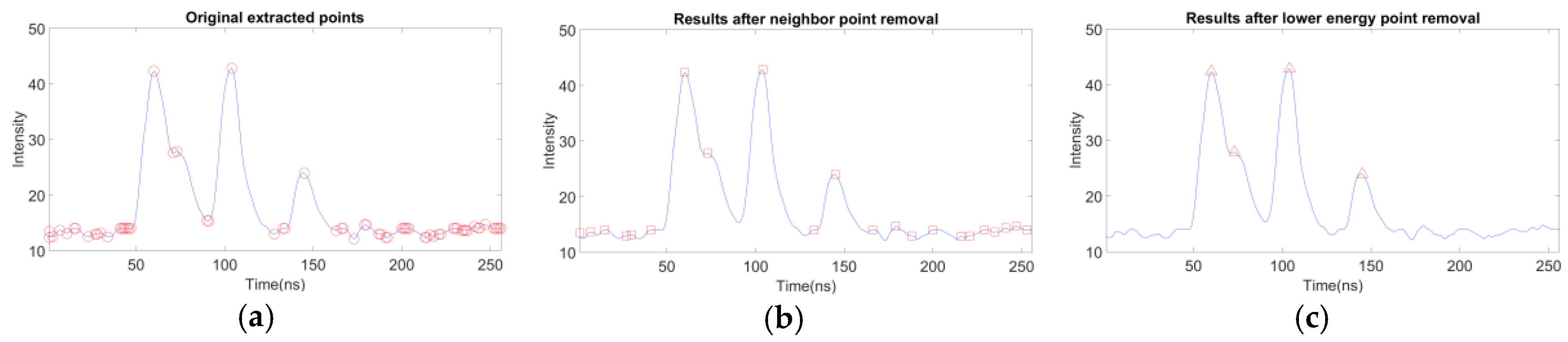
The initial echo detection determines the number and location of peaks for the Gaussian decomposition [21,32]. In the beginning, Gaussian smoothing is applied to reduce the noise effects. Then, a local maximum based on the zero-crossing algorithm [21,33] is used to extract the local maximum points. The refinement conditions are that (1) the local maximum points should be larger than the background noise and (2) the distance between a point and the nearest neighbor point should be larger than a separability threshold. Figure 1 illustrates an example of the initial peak detection and refinement. Figure 1a shows the original extracted points using the zero-crossing algorithm. Figure 1b shows the selected points after removing the nearest neighbor points below the separability threshold. Figure 1c shows the final extracted points after removing the points below the background noise.
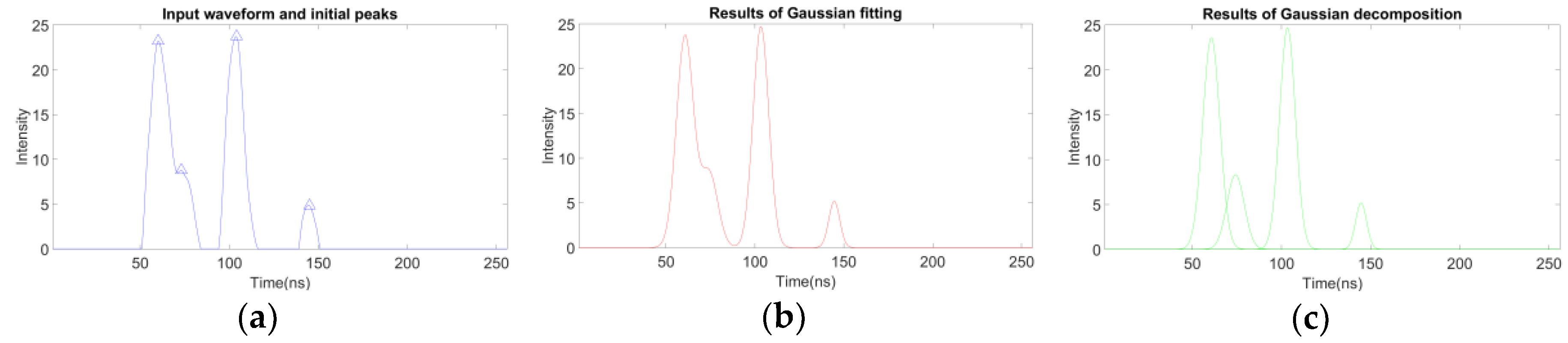
The Gaussian decomposition has the advantage of decreasing the effect of noise and waveform fluctuation [34]. Hence, the Gaussian distribution is selected for this study. Equation (1) is the mathematic model of waveform decomposition using a Gaussian distribution. The received waveform f(t) is a combination of Gaussian functions. After the Gaussian decomposition, waveform parameters such as the position, amplitude, and echo width can be extracted. The position indicates the 3D coordinates of a surface object; the amplitude is the magnitude of the return signals; The echo width is synthetically determined by surface slope and roughness of the target within a laser footprint. Figure 2 illustrates the Gaussian decomposition results. Figure 2a shows the input waveform and initial peaks (i.e., triangles) from the previous step. Figure 2b shows the fitting results using a Gaussian distribution. Figure 2c shows the final result of Gaussian decomposition, and the waveform is decomposed into four spatial objects in this example.
where f(t) is the received signals; t is the round-trip time; ti is the peak’s time of target i; Ai is the amplitude of target i; Wi is the echo width of target i; n is the number of targets.
2.2. Multi-Waveform Processing
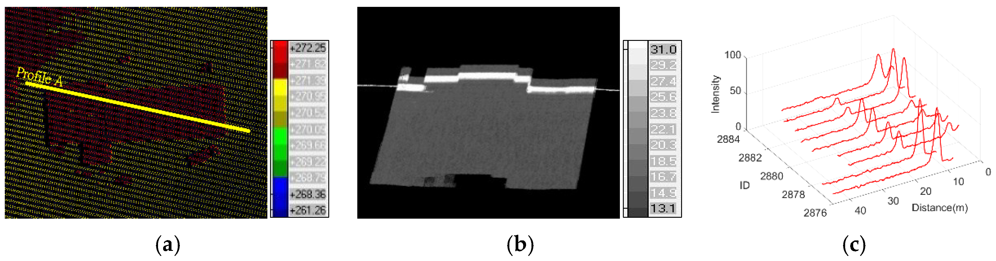
The airborne lidar system acquires data at a small footprint and dense points on the surface. Hence, this study assumes that the adjacent waveforms from a small-footprint lidar system are geospatially correlated. Figure 3a shows the top view of the building lidar points, and Figure 3b shows the corresponding waveform transect. We select a profile that covers building rooftop and ground in Figure 3a to visualize a set of sequential waveforms in the same scanning line. Figure 3b shows the spatial locations of every waveform samples and the samples are colored by waveform strength. In Figure 3b, the neighbor waveforms show similar behavior because they have a higher correlation. Besides, the starting points of each waveform are not the same. The waveform stacking process cannot stack neighbor waveforms directly. The average ground distance between waveform spacing is approximately 70 cm, whereas the footprint is approximately 50 cm in this example. Adjacent waveforms usually have similar return signals in a short distance. The surface object with significant returned signals can be extracted in the single-waveform processing. However, the weak returned signal from the low-penetration object cannot be extracted in the single-waveform processing. This study focuses on the weak return ground points in the forest area. Therefore, only the last echo is extracted in the multi-waveform weak waveform.
The first step of multi-waveform processing is to determine the neighboring waveforms among all waveforms in a mission. There are two possibilities to find the neighboring waveforms: using the GPS time for each waveform and searching through the data to find the nearest waveform via ground distance. The nearest-waveform searching in the ground space is notably time-consuming, so this study uses the GPS time to compare the time difference between waveforms. Figure 3c shows an example of time series waveforms after time sorting in a forest area.
The second step of multi-waveform processing is waveform alignment and stacking. The sampling time interval for the airborne waveform lidar system is commonly 1 ns, which is equivalent to 0.3 m in space considering the round trip for the laser. If the lidar system records the entire signals from air to ground, most signals are going through the air, and the data volume is huge. For example, there are 4000 samples (600 m/0.15 m) at a 600 m flying height for a single pulse. To reduce the data volume and preserve useful signals, the lidar system only provides the waveform from an anchor point to the ground. The data length is commonly 256 samples (256 × 0.15 m = 38.4 m in length), and the anchor points of the pulses do not have identical locations. Each pulse has its own anchor point (X0, Y0, Z0) and directional vector (dX, dY, dZ); the 3D coordinates (X, Y, Z) of every sample in a pulse can be calculated by a scale factor (s) in Equation (2).
where (X, Y, Z) are object coordinates; (X0, Y0, Z0) are the anchor point for each pulse; s is scale factor; (dX, dY, dZ) is the directional vector.
X = X0 + s × dX
Y = Y0 + s × dY
Z = Z0 + s × dZ,
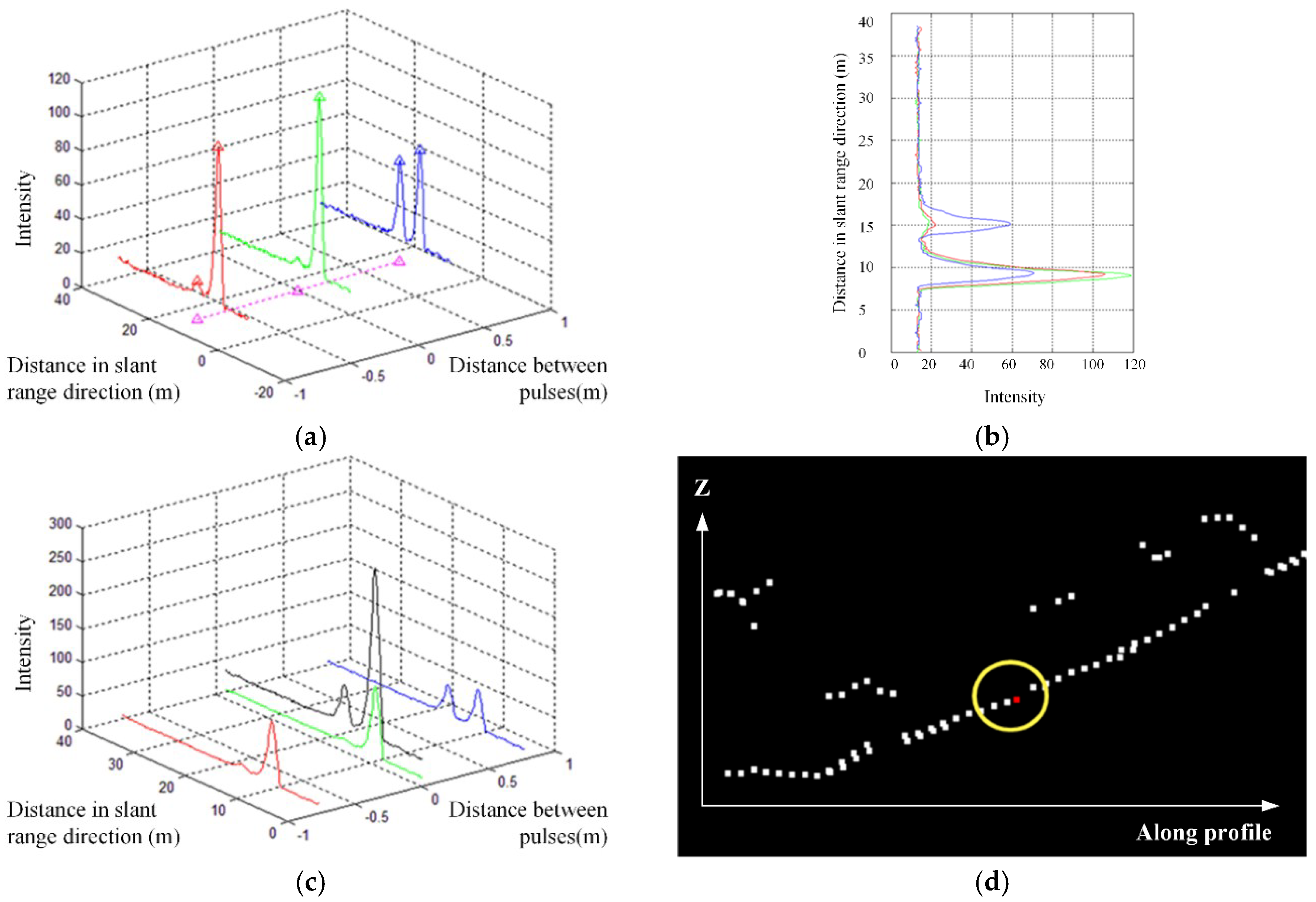
The locations of the anchor points of the pulses slightly vary. Thus, the waveform stacking process cannot directly stack neighbor waveforms (Figure 4a). The waveform alignment is based on the location of the anchor point in the object space to calculate the shifting between waveforms. Assume that the line-of-sights (LOSs) for three sequential pulses in a scan line is a plane, the waveform alignment calculates the perpendicular intersection points between the master and neighboring waveforms. Then, the shifting parameters are calculated from an intersection point and a starting point of a waveform. The precision of shifting parameters is better than 1 sample (e.g., 1 ns). It is used to translate the neighboring waveforms based on the coordinate system of the master waveform. The scanning direction of each pulse is implied on the directional vectors (dX, dY, dZ). Therefore, the impact of scanning angle has been considered in the waveform alignment. As the difference of scanning angles between adjacent waveforms is very small (e.g., less than 0.02 degrees), the scanning angles of adjacent waveforms can be assumed as parallel to each other. The shifting direction is the pointing direction of each waveform. The waveform stacking simply translates a neighbor waveform to align the master and neighbor waveforms (Figure 4b).
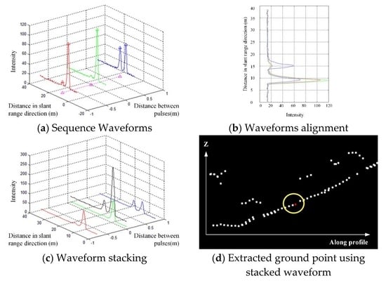
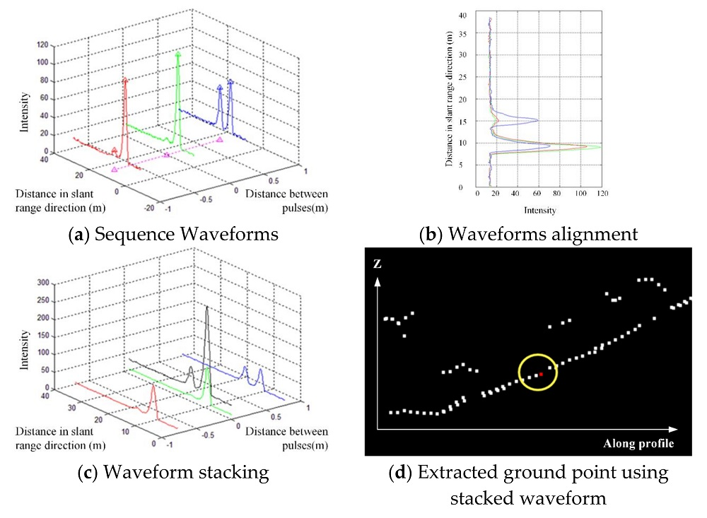
After the waveforms have been aligned, the master and adjacency waveforms are combined into a stacked waveform. As all the waveforms are aligned in slant range direction, the waveform stacking takes the average of master and neighbor waveforms based on the corresponding location. Figure 4c shows an example of waveform alignment and stacking. The green waveform is the master waveform to enhance, whereas the blue and red waveforms are adjacent waveforms. These three waveforms are combined into a stacked waveform after alignment and stacking. The stacking result is the black waveform. Finally, Gaussian decomposition is applied to extract the peak location of the weak returns. To compare the original waveform (Green) and stacked waveform (Black), the weak signal of the last echo in the original waveform can be enhanced by adjacent waveforms after stacking.
The last step of multi-waveform processing is Gaussian decomposition, as mentioned in Section 2.1. The Gaussian decomposition extracts several echoes from the stacked waveform. The multi-waveform processing technique only considers the last echo (Figure 4d) because the first and intermedium echoes have been extracted in the single-waveform processing. Another reason is that the weak echo commonly occurs in the last return caused by the low penetration rate. The proposed method assumes that the weak return is the last return. Only the return usually has a higher strength and will not be considered as a weak return. For the stacked waveform that only has one peak, this peak has been extracted in the single waveform extraction and will not be considered as an additional point for verification.
2.3. Verification of the Enhanced Weak Last Return
The multi-waveform processing technique is applied to all sequential waveforms. To avoid redundancy and incorrect echoes, this study designs three criteria by comparing the results of single-waveform processing and multi-waveform processing. The results of the master waveform include the echoes from single-waveform processing and the last echo from the multi-waveform processing. If the peak location from these two methods is smaller than a predefined threshold (i.e., 2.5σ = 2.5 × 0.3 m = 0.75 m), these two echoes are considered as the same echo, and we remove the result from the multi-waveform processing. This verification can remove redundancy. The results of the neighbor waveforms are not included in this verification.
The second criterion compares the last echo from the multi-waveform method and the two last echoes from the two neighbor waveforms in the single-waveform method. To ensure that the last echoes from two neighbor waveforms cover the same object, we assume that the terrain relief in a short distance is smooth, and the vertical distance between these two last echoes should be less than a vertical threshold T1 of 3 m. After the waveform alignment, the last echoes from two neighbor waveforms can be linked to a line, and the intersection between the linked line and the master waveform is a pseudo echo for verification. If the distance between the pseudo echo and last echo from multi-waveform method is larger than a predefined threshold (i.e., 2.5σ = 2.5 × 0.3 m = 0.75 m), the extracted last echo will be far away from this pseudo echo and is considered as an incorrect echo.
The last criterion evaluates that the last echo from the multi-waveform method is a ground point. Commonly, the distance between the tree crown (e.g., the first return) and a ground point (e.g., the last return) is relatively large. The ground point under the tree crown is commonly a weak return for multi-waveform processing. If the vertical distance between the first and the last echoes in the multi-waveform method is smaller than a vertical threshold T2 of 2.25 m, the last echo is considered a non-ground point and we remove the result from the multi-waveform method.
2.4. Accuracy Assessment
The evaluations were performed in four steps. First, we considered the correctness of different vertical thresholds in the verification of the enhanced weak last return. The correctness was verified by manual editing and defined by Equation (3). Second, we compared the enhanced weak last return covering with different forest complexities. The correctness and increasing rate were selected to compare the results from the original point clouds, single-waveform processing, and multi-waveform. The increasing rate is the number ratio of original and enhanced ground points (Equation (4)). Third, we analyzed the effect of the distance between neighbor and master waveforms. To discuss the geospatial-related waveforms in different distances, we used the correctness to evaluate the overall performance in different spatial distances. The last part analyzed the effect of the sampling length per waveform. The different lidar systems provide different numbers of the sample length, for example, 256 samples for Leica system and 100 samples for Rigel system in this study. We assessed the correctness from different sampling lengths per waveform.
where C% is the correctness in percentage; NGC is the number of correct ground points; NGT is the total number of ground points; I% is the increasing rate; NGM is the number of ground points from multi-waveform processing; NGO is the number of ground points before multi-waveform processing.
C% = NGC/NGT,
I% = NGM/NGO,
3. Test Data
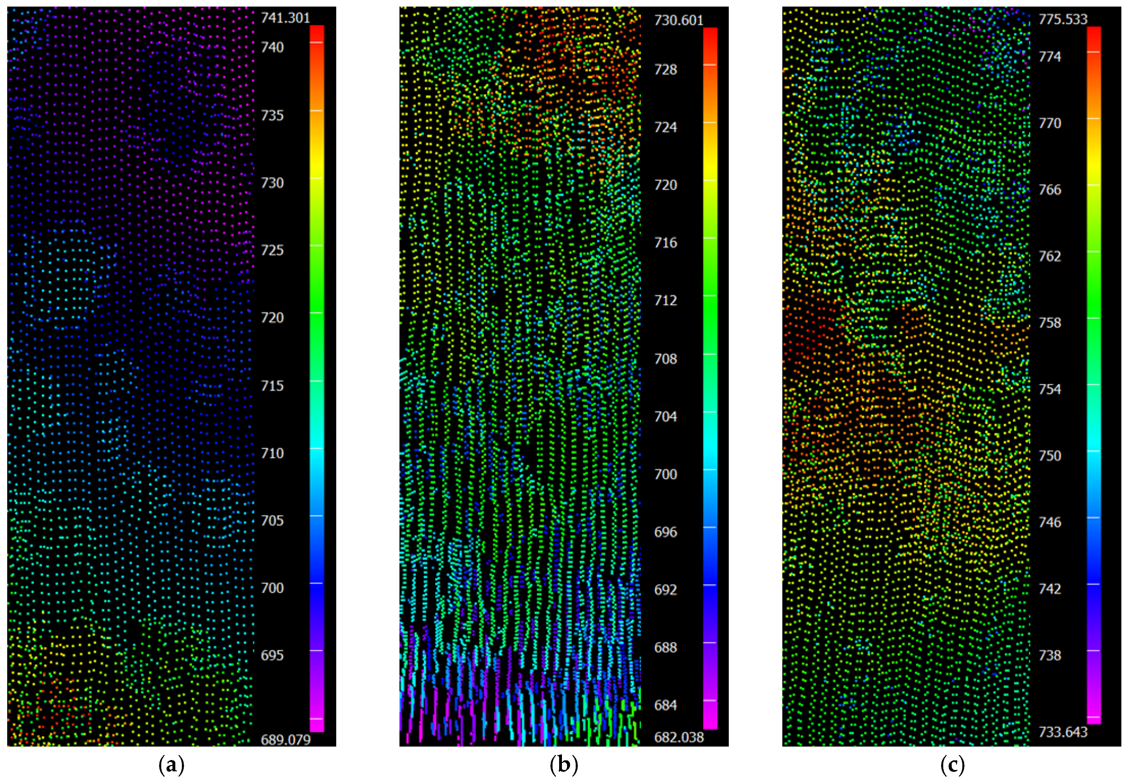
The test area is a forest area in central Taiwan; three areas with different tree complexities were selected to evaluate the proposed method. The size of each test area was 20 m by 60 m. Table 1 summarizes the parameters of the test area. The tree densities for areas 1, 2 and 3 are low, medium and high, respectively. Area 1 has relatively lower tree heights (3–15 m) than other areas (3–23 m). Area 3 contains multilayer vegetation and has a relatively lower penetration rate than other areas. For area 1, the waveform lidar data were acquired by Leica ALS60, Optech Pegasus, and Riegl Q680i, respectively. For areas 2 and 3, only the waveform lidar from Leica ALS60 is available. Figure 5 shows the original lidar points for these three areas. All data were recorded in the format of LAS1.3 [35] with waveform information. The dataset of Leica and Riegl used the regular number of sample for a waveform. The numbers of sample per waveform for Leica and Riegl are 256 samples and 100 samples at 1 nano-sec sampling interval, respectively. These numbers are equivalent to 38.4 m and 15 m in the slant range. To reduce the data volume, the Optech dataset provides different numbers of samples (56–216 samples) in length for different pulses. The number of the sample is equivalent to 8.4–32.4 m. Since the tree height in area 1 is less than 15 m, the waveform data from these three sensors can cover from the treetop to the ground. We selected area 1 to compare the results from these three sensors.
4. Results
4.1. Analysis of Vertical Thresholds
Cases 1, 2, and 3 were used in the threshold analysis. The correctness and number of the correct point were manually evaluated by profiling the lidar points in the TerraScan software. We used two vertical thresholds (T1 and T2) in the verification of the enhanced weak last return. Threshold T1 evaluates that the last echoes from two neighbor waveforms cover the same object, whereas threshold T2 evaluates that the last echo from the multi-waveform method is a ground point. According to the tree height and topography elevation, the initial thresholds T1 and T2 are defined as 3 ± 1.5 m and 2.25 ± 0.75 m, respectively.
Table 2 shows the results of the correctness and number of correct points using different thresholds T1 (i.e., 4.5 m, 3 m and 1.5 m). T2 was fixed as 2.25 m in the evaluation of T1. Because the local terrain relief in sequential pulses was small, the vertical distance of 4.5 m between two last echoes produced a low correctness (53–64%) compared to other thresholds. Although the threshold 1.5 m has a higher correctness, it has fewer correct ground points than other thresholds. Therefore, we selected 3 m for threshold T1 to preserve both correctness and the number of correct points.
Table 3 shows the results using different threshold T2 values (i.e., 3 m, 2.25 m, and 1.5 m). T1 was fixed as 3 m in the evaluation of T2. We assumed that the weak return (e.g., ground) was under the tree crown. Hence, the distance between the enhanced last echo and the first echo should be larger than T2. The threshold T2 evaluates that the extracted pulse is from the ground, and this parameter was obtained based on the smallest height of vegetation in the test area. The threshold of 1.5 m generated many incorrect ground points than other thresholds, so it had a lower correctness than the other parameters. However, the threshold of 3 m produced fewer correct points. Overall, the threshold of 2.25 m showed the highest correctness among all parameters. Therefore, we selected 2.25 m for threshold T2 to preserve both correctness and the number of correct points.
4.2. Comparison of Different Forest Densities
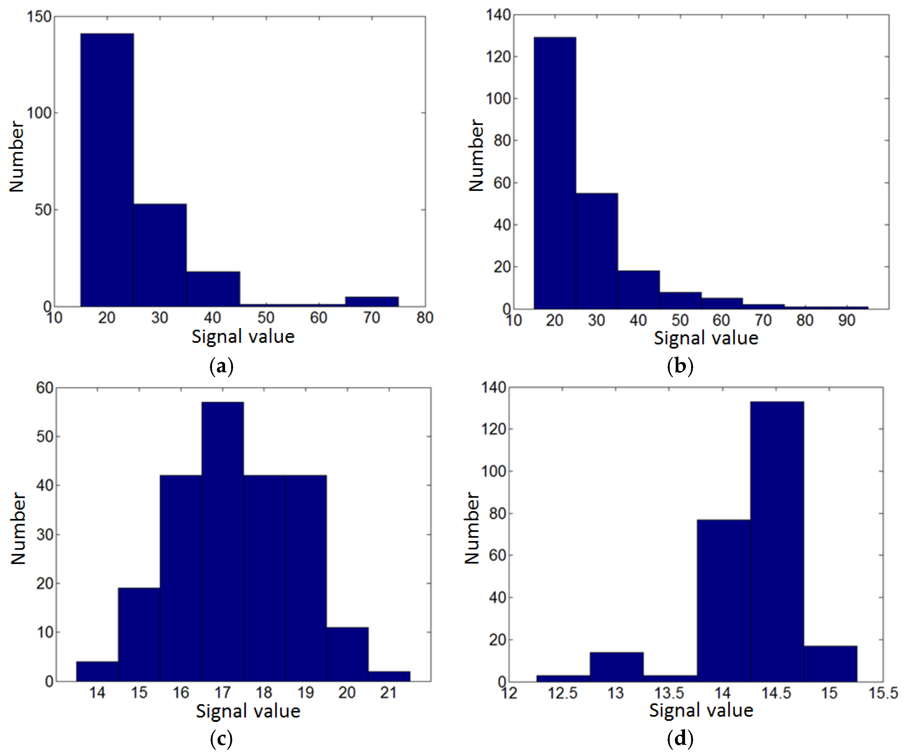
This section uses cases 1, 2, and 3 to analyze the results from different complexities. To demonstrate the low return signal from the enhanced last echo using multi-waveform processing, this section compared the intensity of the last extracted echo between adjacent waveforms (Figure 6a,b), master waveform (Figure 6c) and background noise of the master waveform (Figure 6d). Figure 6 shows the intensity histogram, where the x-axis and y-axis are the intensity and number of echoes, respectively. Figure 6c shows the intensity of the extracted last echo using the proposed multi-waveform processing. The adjacent waveforms show higher strength (20–70 and 20–90) than the master waveform (14–21). Thus, the proposed waveform stacking can enhance the weak return using adjacent waveforms. The weak return of the master waveforms was 14–21 and overlapped with the background noise level (12.5–15). This weak return was not easy to extract via single-waveform processing when it was similar to the background noise. Thus, the proposed method can extract the weak returns on the ground when we consider the geospatial relationships.
Table 4 shows the statistical results to compare the ground points of the original dataset, single-waveform processing, and multi-waveform processing. The single-waveform processing extracts both ground and non-ground points, whereas multi-waveform method only considers the ground points. The numbers of ground points from the original dataset and single-waveform processing were manually identified. The increasing rate is the number ratio of the increased points and original ground points. The increasing rates of single-waveform processing were +18–59%, which are similar to the previous study [16,36]. The multi-waveform method could extract additional weak ground points (+3–12%) after the traditional single-waveform processing. The multi-waveform method extracted the last return as a ground point, and the evaluation shows that the correctness was above 76% in the three cases.
To compare the complexities in these three cases, case 1 shows a lower tree crown coverage because it has the highest percentage of ground points (55%). Because of the lower tree coverage, case 1 also has a lower increasing rate (+18% and +3%) after single- and multi-waveform processing. The number of increased ground points is related to the pulse density, whereas the increasing rate is related to the penetration rate. Case 3 has a lower penetration rate as the percentage of the ground point was only 9%. Therefore, the single-waveform and multi-waveform methods effectively increased the number of ground points and the increasing rate in case 3 (+59% and +26%). Thus, the proposed method helps to increase the percentage of ground points compared to discrete lidar. These three cases had similar trends of the increasing rate for single- and multi-waveform processing. Moreover, the correctness of the multi-waveform method was 76% for all cases.
4.3. Comparison of Different Spatial Distances between Waveforms
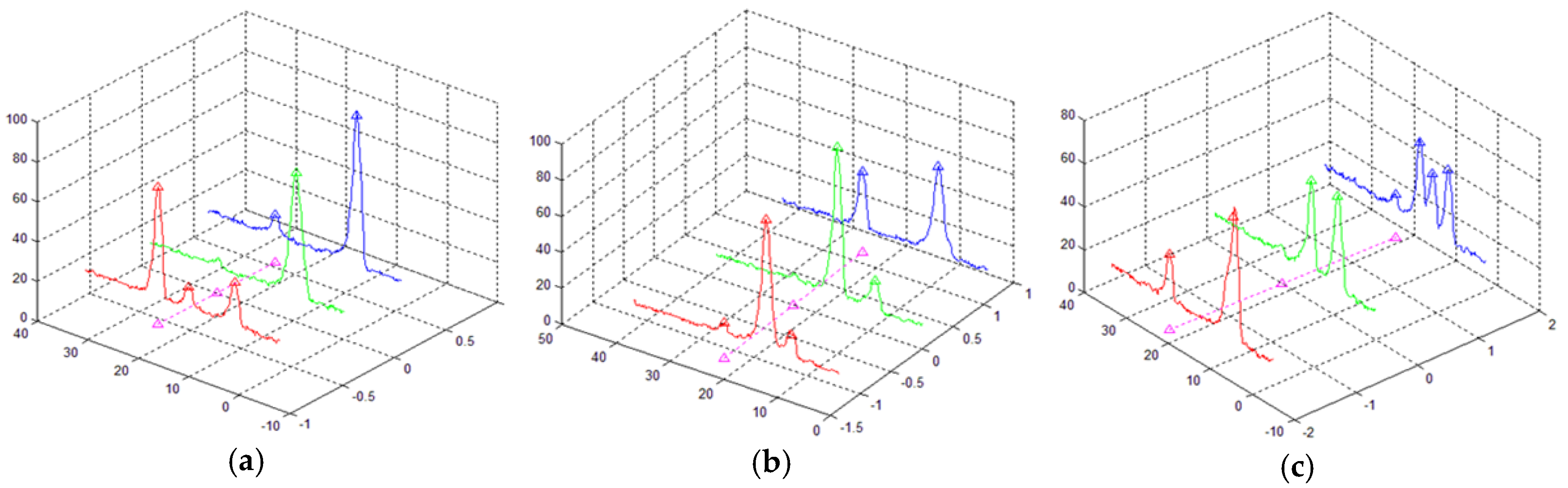
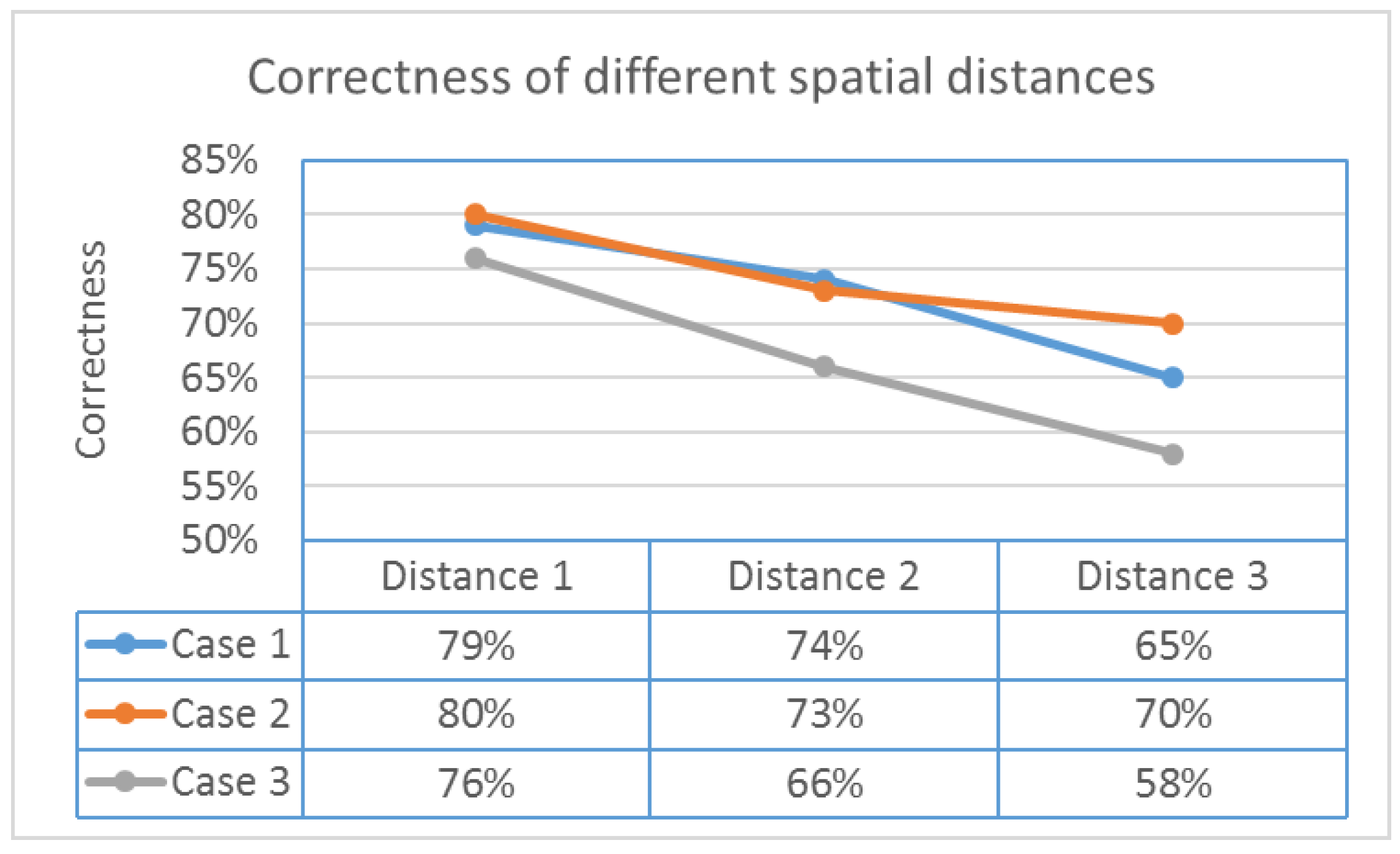
This section uses cases 1–3 to analyze the effect of the adjacent waveform selection in different spatial distances. We designed three spatial distances in waveform stacking. Distance 1 selected two nearest waveforms; distances 2 and 3 were the 2nd and 3rd neighbor waveforms. The spatial distances for distances 1–3 were 0.4–0.7 m, 0.7–1.4 m, and 1.4–2.1 m, respectively (Figure 7). The correctness of the ground point from different spatial distances is shown in Figure 8. The results show that the nearest waveforms have higher correlation; consequently, distance 1 had the highest correctness among the three distances. For a complex area such as case 3, the correctness was reduced from 76% to 58%. In summary, the larger spatial distance may reduce the correctness. Therefore, this study suggests considering the nearest waveforms such as distance 1 in waveform stacking.
4.4. Comparison of Different Sampling Numbers of Waveform
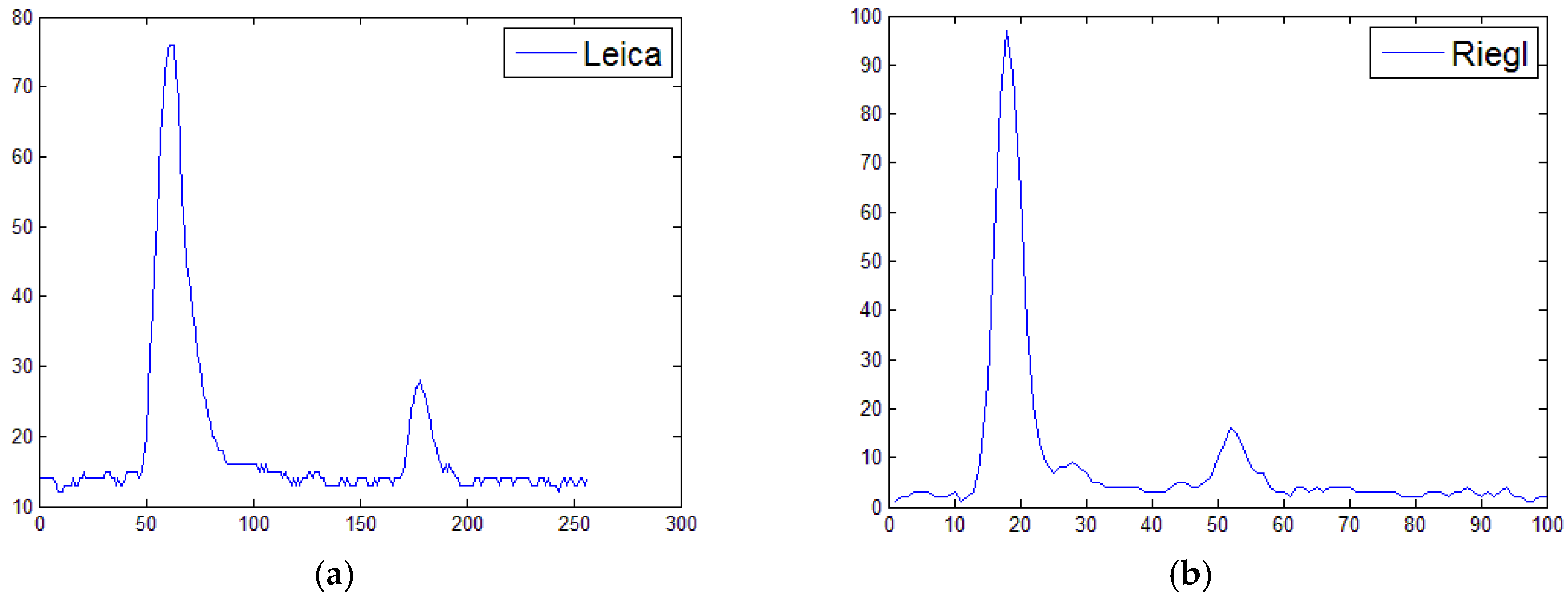
We also analyzed the effects of different sampling numbers per waveform. Cases 1, 4, and 5 were located in the same area but had different numbers of samples. Cases 1 and 4 had 256 samples and 100 samples at 1 ns sample interval, and the corresponding spatial lengths were 38.4 m and 15 m, respectively. Case 5 provides different numbers of samples (56–216 samples) according to the different objects. Figure 9 shows different waveforms from cases 1 and 4. In Figure 9a, the time difference between the first return and the last return was 115 ns (17.25 m). In Figure 9b, the time difference between the first return and the last return was 30 ns (4.5 m). Figure 9 demonstrates that the larger sampling number covers more comprehensive information than the smaller one. The available sampling number per waveform is the limitation of using LAS 1.3 in this study, which can be overcome by using the data before converting to LAS, e.g., the SDF file format from the Riegl system.
Table 5 compares the results using different sampling numbers. Because of the length of the sampling number, case 4 has the lowest increasing point from single-waveform processing and multi-waveform processing. The results show that the sampling numbers per waveform are an important factor to cover from the treetop to the ground. A comparison of the results of single-waveform processing for the three cases shows that case 1 had more increased points (+325 points) than the other cases. The original points of case 1 were extracted from the return signals using a simple thresholding algorithm. Therefore, the Gaussian decomposition in single-waveform processing significantly extracts the ground points.
Although case 5 had only 50 increased ground points after the single-waveform processing, it had the largest number of increased ground points using the multi-waveform method (+158 points). This result shows the benefit of using dual laser systems in different acquisition directions for the Optech Pegasus system; different scanning directions increase the possibilities of penetration in the forest area. Hence, the multi-waveform method for case 5 effectively extracted more weak ground than other cases. In addition, the dynamic sampling numbers for case 5 may reduce the file size and preserve the capability of weak waveform enhancement. Overall, the correctness of the proposed method was 76–78% in different cases. Thus, the proposed method can provide stable correctness from different sampling numbers.
5. Conclusions and Future Works
This study proposed a multi-waveform processing technique to extract weak returns. We assume that adjacent waveforms are geospatially correlated and have similar waveform properties, which can be used to validate the correctness of the extracted echo. The major contributions of this study are the (1) establishment of a geospatial-related waveforms analysis to extract weak returns; (2) the comparison of the results of single-waveform and multi-waveform processing; and (3) the evaluation of the effect of different sampling numbers per waveform from different lidar systems. The proposed scheme integrates sequential waveforms to identify the weak return and subsequently improves the number of ground points in the forest area.
This study concludes that (1) the proposed method can extract the weak returns, which are similar to the background noise; (2) The nearest waveforms have a higher correlation, so the integration of nearest waveforms shows a higher correctness. The correctness was 76–80% for cases 1–3; (3) To compare the sampling numbers per waveform, the shortest sampling number has the lowest increasing point from both single-processing and multi-waveform processing. The sampling number per waveform is one of the key factors for the proposed method.
The aim of this study is to redetect the partially occluded weak return by multi-waveform processing. The waveform staking is to enhance the partially weak return from the ground surface. If the crown layer occurs within waveform spacing and the progressive waveforms are totally occluded by the tree crown, the waveform staking will extract the additional point on the crown cover but not the ground surface. Hence, the limitation of the proposed method is to not be able to enhance the ground surface totally occluded by the tree crown.
The proposed method assumed that the sequential waveforms along the scanning direction have a higher correlation. The synthetic waveform was combined by sequential waveforms in the same scan line and the adjacent waveforms between scan lines were not considered in the waveform stacking. In order to gain more spatial neighboring information, future works will focus on examining different adjacent waveforms from different scan lines for a 3D synthetic waveform.
Author Contributions
T.-A.T. provided the overall conception of this research, designs the methodologies and experiments, and wrote the majority of the manuscript; W.-Y.Y. contributed to the implementation of proposed algorithms, conducts the experiments and performs the data analyses.
Funding
This research was funded by Ministry of Science and Technology of Taiwan grant number NSC 101-2628-E-009-019-MY3.
Acknowledgments
The authors would also like to thank the Ministry of Interior and LIDAR Technology Co., Ltd. in Taiwan for providing the test datasets for experiments.
Conflicts of Interest
The authors declare no conflict of interest.
References
- Maune, D.F. DEM User Application, Digital Elevation Model Technologies and Applications: The DEM Users Manual, 2nd ed.; Maune, D.F., Ed.; The American Society for Photogrammetry and Remote Sensing: Bethesda, MD, USA, 2007; pp. 391–423. [Google Scholar]
- Yan, W.Y.; Shaker, A.; El-Ashmawy, N. Urban land cover classification using airborne LiDAR data: A review. Remote Sens. Environ. 2015, 158, 295–310. [Google Scholar] [CrossRef]
- Čeru, T.; Šegina, E.; Gosar, A. Geomorphological dating of Pleistocene conglomerates in central Slovenia based on spatial analyses of dolines using lidar and ground penetrating radar. Remote Sens. 2017, 9, 1213. [Google Scholar] [CrossRef]
- Wu, J.Y.; Teo, T.A.; Shih, P.T.Y. Geomorphological change detection using an integrated method: A case study of Taan River Watershed, Taiwan. Terr. Atmos. Ocean. Sci. 2016, 27, 521–536. [Google Scholar] [CrossRef]
- Lim, K.; Treitz, P.; Wulder, M.; St-Onge, B.; Flood, M. LiDAR remote sensing of forest structure. Prog. Phys. Geogr. 2003, 27, 88–106. [Google Scholar] [CrossRef]
- Toth, C.K.; Petrie, G. Topographic Laser Ranging and Scanning: Principles and Processing, 2nd ed.; Taylor & Francis, CRC Press: Oxford, UK, 2018. [Google Scholar]
- Hovi, A.; Korhonen, L.; Vauhkonen, J.; Korpela, I. LiDAR waveform features for tree species classification and their sensitivity to tree-and acquisition related parameters. Remote Sens. Environ. 2016, 173, 224–237. [Google Scholar] [CrossRef]
- Milenković, M.; Wagner, W.; Quast, R.; Hollaus, M.; Ressl, C.; Pfeifer, N. Total canopy transmittance estimated from small-footprint, full-waveform airborne LiDAR. ISPRS J. Photogramm. Remote Sens. 2017, 128, 61–72. [Google Scholar] [CrossRef]
- Adams, T.; Beets, P.; Parrish, C. Extracting more data from lidar in forested areas by analyzing waveform shape. Remote Sens. 2012, 4, 682–702. [Google Scholar] [CrossRef]
- Yao, W.; Stilla, U. Mutual enhancement of weak laser pulses for point cloud enrichment based on full-waveform analysis. IEEE Trans. Geosci. Remote Sens. 2010, 48, 3571–3579. [Google Scholar] [CrossRef]
- Persson, Å.; Söderman, U.; Töpel, J.; Ahlberg, S. Visualization and analysis of fullwaveform airborne laser scanner data. Int. Arch. Photogramm. Remote Sens. Spat. Inf. Sci. 2005, 36, 103–108. [Google Scholar]
- Jutzi, B.; Neulist, J.; Stilla, U. Sub-pixel edge localization based on laser waveform analysis. Int. Arch. Photogramm. Remote Sens. Spat. Inf. Sci. 2005, 36, 12–14. [Google Scholar]
- Michelin, J.C.; Mallet, C.; David, N. Building edge detection using small-footprint airborne full-waveform lidar data. ISPRS Ann. Photogramm. Remote Sens. Spat. Inf. Sci. 2012, 1, 147–152. [Google Scholar] [CrossRef]
- Słota, M. Full-waveform data for building roof step edge localization. ISPRS J. Photogramm. Remote Sens. 2015, 106, 129–144. [Google Scholar] [CrossRef]
- Tseng, Y.H.; Wang, C.K.; Chu, H.J.; Hung, Y.C. Waveform-based point cloud classification in land-cover identification. Int. J. Appl. Earth Obs. Geoinf. 2015, 34, 78–88. [Google Scholar] [CrossRef]
- Chauve, A.; Vega, C.; Durrieu, S.; Bretar, F.; Allouis, T.; Pierrot Deseilligny, M.; Puech, W. Advanced full-waveform lidar data echo detection: Assessing quality of derived terrain and tree height models in an alpine coniferous forest. Int. J. Remote Sens. 2009, 30, 5211–5228. [Google Scholar] [CrossRef] [Green Version]
- Toth, C.K.; Zaletnyik, P.; Laky, S.; Grejner-Brzezinska, D.A. Peak detection from full-waveform data. In Proceedings of the International LiDAR Mapping Forum, Salzburg, Austria, 29–30 November 2011. [Google Scholar]
- Abshire, J.B.; McGarry, J.F.; Pacini, L.K.; Balair, J.B.; Elman, G.C. Laser Altimetry Simulator Version 3.0 User's Guide; Technical Memorandum 104588; National Aeronautics and Space Administration: Washington, DC, USA, 1994; p. 66.
- Słota, M. Advanced processing techniques and Classification of full-waveform airborne laser scanning data. Geomat. Environ. Eng. 2014, 8, 85–95. [Google Scholar] [CrossRef]
- Ullrich, A.; Pfennigbauer, M. Echo digitization and waveform analysis in airborne and terrestrial laser scanning. Photogramm. Week 2011, 11, 217–228. [Google Scholar]
- Wagner, W.; Ullrich, A.; Ducic, V.; Melzer, T.; Studnicka, N. Gaussian decomposition and calibration of a novel small-footprint full-waveform digitising airborne laser scanner. ISPRS J. Photogramm. Remote Sens. 2006, 60, 100–112. [Google Scholar] [CrossRef]
- Lin, Y.-C.; Mills, J.P.; Smith-Voysey, S. Rigorous pulse detection from full-waveform airborne laser scanning data. Int. J. Remote Sens. 2010, 31, 1303–1324. [Google Scholar] [CrossRef]
- Salas, E.A.L.; Henebry, G.M. Canopy height estimation by characterizing waveform lidar geometry based on shape-distance metric. AIMS Geosci. 2016, 2, 366–390. [Google Scholar] [CrossRef]
- Salas, E.A.L.; Amatya, S.; Henebry, G.M. Application of iterative noise-adding procedures for evaluation of moment distance index for lidar waveforms. AIMS Geosci. 2017, 3, 187–215. [Google Scholar] [CrossRef]
- Mallet, C.; Lafarge, F.; Bretar, F.; Roux, M.; Soergel, U.; Heipke, C. A stochastic approach for modelling airborne lidar waveforms. Int. Arch. Photogramm. Remote Sens. Spat. Inf. Sci. 2009, 38, 201–206. [Google Scholar]
- Brenner, A.C.; Zwally, H.J.; Bentley, C.R.; Csatho, B.M.; Harding, D.J.; Hofton, M.A.; Minster, J.; Roberts, L.; Saba, J.L.; Thomas, R.H. The Algorithm Theoretical Basis Document for the Derivation of Range and Range Distributions from laser Pulse Waveform Analysis for Surface Elevations, roughness, Slope, and Vegetation Heights; National Aeronautics and Space Administration: Washington, DC, USA, 2012; p. 126.
- Wang, C.K. Exploring weak and overlapped returns of a lidar waveform with a wavelet-based echo detector. Int. Arch. Photogramm. Remote Sens. Spatial Inf. Sci. 2012, 39, 529–534. [Google Scholar] [CrossRef]
- Hu, B.; Gumerov, D.; Wang, J.; Zhang, W. An integrated approach to generating accurate DTM from airborne full-waveform lidar data. Remote Sens. 2017, 9, 871. [Google Scholar] [CrossRef]
- Pirotti, F. Analysis of full-waveform lidar data for forestry applications: A review of investigations and methods. iForest 2011, 4, 100–106. [Google Scholar] [CrossRef]
- Reitberger, J.; Krzystek, P.; Stilla, U. Analysis of full waveform lidar data for the classification of deciduous and coniferous trees. Int. J. Remote Sens. 2008, 29, 1407–1431. [Google Scholar] [CrossRef]
- Bater, C.W.; Coops, N.C. Evaluating error associated with lidar-derived DEM interpolation. Comput. Geosci. 2009, 35, 289–300. [Google Scholar] [CrossRef]
- Hofton, M.A.; Minster, J.B.; Blair, J.B. Decomposition of laser altimeter waveforms. IEEE Trans. Geosci. Remote Sens. 2000, 38, 1989–1996. [Google Scholar] [CrossRef]
- Wagner, W.; Ullrich, A.; Melzer, T.; Briese, C.; Kraus, K. From single-pulse to full-waveform airborne laser scanners: Potential and practical challenges. Int. Arch. Photogramm. Remote Sens. Spat. Inf. Sci. 2004, 35, 201–206. [Google Scholar]
- Jutzi, B.; Stilla, U. Range determination with waveform recording laser systems using a Wiener Filter. ISPRS J. Photogramm. Remote Sens. 2006, 61, 95–107. [Google Scholar] [CrossRef]
- Aerial Photography Summary Record System. Las Specification Version 1.3-R10; The American Society for Photogrammetry and Remote Sensing: Bethesda, MD, USA, 2009; p. 17. [Google Scholar]
- Wang, C.K.; Tseng, Y.H.; Wang, C.K. A wavelet-based echo detector for waveform LiDAR data. IEEE Trans. Geosci. Remote Sens. 2016, 54, 757–769. [Google Scholar] [CrossRef]
Figure 1.
The illustration of initial peaks’ detection: (a) Original extracted points; (b) Results after neighbor point removal; (b) Results after lower energy point removal.
Figure 1.
The illustration of initial peaks’ detection: (a) Original extracted points; (b) Results after neighbor point removal; (b) Results after lower energy point removal.

Figure 2.
The illustration of Gaussian decomposition: (a) Input waveform and initial peaks; (b) Results of Gaussian fitting; (b) Results of Gaussian decomposition.
Figure 2.
The illustration of Gaussian decomposition: (a) Input waveform and initial peaks; (b) Results of Gaussian fitting; (b) Results of Gaussian decomposition.

Figure 3.
The illustration of the sequential waveforms: (a) Top view of lidar point clouds and colored by height in meter (the color bar indicate the height in meters); (b) Profile of sequential waveforms (the color bar indicate the intensity); (c) Sequential-waveform-covered tree.
Figure 3.
The illustration of the sequential waveforms: (a) Top view of lidar point clouds and colored by height in meter (the color bar indicate the height in meters); (b) Profile of sequential waveforms (the color bar indicate the intensity); (c) Sequential-waveform-covered tree.

Figure 4.
The illustration of multi-waveform processing: (a) Sequence Waveforms; (b) Result of waveforms alignment; (c) Result of waveform stacking (black color waveform is stacked waveform); (d) Result of extracted ground point using stacked waveform.
Figure 4.
The illustration of multi-waveform processing: (a) Sequence Waveforms; (b) Result of waveforms alignment; (c) Result of waveform stacking (black color waveform is stacked waveform); (d) Result of extracted ground point using stacked waveform.

Figure 5.
The original lidar points from Leica ALS60: (a) Area 1 with lower tree density; (b) Area 2 with medium tree density; (c) Area 3 with higher tree density.
Figure 5.
The original lidar points from Leica ALS60: (a) Area 1 with lower tree density; (b) Area 2 with medium tree density; (c) Area 3 with higher tree density.

Figure 6.
The histogram of waveform strength: (a) The histogram of adjacent waveforms at time t − 1; (b) The histogram of adjacent waveforms at time t + 1; (c) The histogram of master waveforms at time t; (d) The background noise of master waveforms at time t.
Figure 6.
The histogram of waveform strength: (a) The histogram of adjacent waveforms at time t − 1; (b) The histogram of adjacent waveforms at time t + 1; (c) The histogram of master waveforms at time t; (d) The background noise of master waveforms at time t.

Figure 7.
The different spatial distances: (a) Distance 1: 0.4–0.7 m; (b) Distance 2: 0.7–1.4 m; (c) Distance 3: 1.4–2.1 m.
Figure 7.
The different spatial distances: (a) Distance 1: 0.4–0.7 m; (b) Distance 2: 0.7–1.4 m; (c) Distance 3: 1.4–2.1 m.

Figure 8.
The correctness of different spatial distances.

Figure 9.
The different waveforms in this study: (a) a waveform with 256 samples from case 1; (b) a waveform with 100 samples from case 4.
Figure 9.
The different waveforms in this study: (a) a waveform with 256 samples from case 1; (b) a waveform with 100 samples from case 4.


Table 1.
The summary of the test data.
| Items | Case 1 | Case 2 | Case 3 | Case 4 | Case 5 |
|---|---|---|---|---|---|
| Area | Area 1 | Area 2 | Area 3 | Area 1 | Area 1 |
| Sensor | Leica ALS60 | Leica ALS60 | Leica ALS60 | Riegl Q680i | Optech Pegasus |
| Flying height | 2900 m AGL | 2900 m AGL | 2900 m AGL | 2600 m AGL | 1100 m AGL |
| Laser pulse rate (kHz) | 55 | 55 | 55 | 220 | 100 |
| Scanning rate (Hz) | 61 | 61 | 61 | 119 | 35 |
| Date | October 2011 | October 2011 | October 2011 | January 2012 | October 2011 |
| Number of sample per waveform | 256 | 256 | 256 | 100 | 56–216 |
| Sampling interval | 1 ns | 1 ns | 1 ns | 1 ns | 1 ns |
| Average point density (pts/m2) | 3 | 9 | 5 | 2 | 3.5 |
| Average distance between waveforms (m) | 0.77 | 0.61 | 0.70 | 0.80 | 0.75 |
| Tree height (m) | 3–15 | 3–22 | 3–23 | 3–15 | 3–15 |
| Elevation (m) | 689–741 | 682–730 | 733–775 | 689–741 | 689–741 |
Table 2.
The analysis of threshold T1.
| 4.5 m | 3.0 m | 1.5 m | ||||
|---|---|---|---|---|---|---|
| Correct Points | Correctness (%) | Correct Points | Correctness (%) | Correct Points | Correctness (%) | |
| Case 1 | 48 | 53 | 48 | 79 | 41 | 83 |
| Case 2 | 197 | 64 | 197 | 80 | 190 | 85 |
| Case 3 | 101 | 54 | 101 | 76 | 89 | 82 |
Table 3.
The analysis of threshold T2.
| 3.0 m | 2.25 m | 1.5 m | ||||
|---|---|---|---|---|---|---|
| Correct Points | Correctness (%) | Correct Points | Correctness (%) | Correct Points | Correctness (%) | |
| Case 1 | 39 | 76 | 48 | 79 | 48 | 71 |
| Case 2 | 177 | 80 | 197 | 80 | 197 | 76 |
| Case 3 | 84 | 71 | 101 | 76 | 102 | 64 |
Table 4.
The comparison between different complexities.
| Case 1 | Case 2 | Case 3 | ||
|---|---|---|---|---|
| Original (all points) | 3309 | 10610 | 5902 | |
| Original ground points | Ground points | 1810 | 2135 | 508 |
| Percentage | 55% | 20% | 9% | |
| After single waveform processing | Increased point | +325 | +988 | +301 |
| Increasing rate | +18% | +46% | +59% | |
| After multi-waveform processing | Increased point | +61 | +247 | +133 |
| Increasing rate | +3% | +12% | +26% | |
| Correct point | 48 | 197 | 101 | |
| Correctness | 79% | 80% | 76% | |
Table 5.
The comparison between different sampling numbers.
| Case 1 | Case 4 | Case 5 | ||
|---|---|---|---|---|
| Number of sample per waveform | 256 | 100 | 56–216 | |
| Original (all points) | 3309 | 2396 | 4177 | |
| Original ground points | Ground points | 1810 | 1290 | 1920 |
| Percentage | 55% | 54% | 47% | |
| After single waveform processing | Increased point | +325 | +59 | +50 |
| Increasing rate | +18% | +5% | +3% | |
| After multi-waveform processing | Increased point | +61 | +33 | +158 |
| Increasing rate | +3% | +3% | +8% | |
| Correct point | 48 | 25 | 123 | |
| Correctness | 79% | 76% | 78% | |
© 2018 by the authors. Licensee MDPI, Basel, Switzerland. This article is an open access article distributed under the terms and conditions of the Creative Commons Attribution (CC BY) license (http://creativecommons.org/licenses/by/4.0/).
Share and Cite
MDPI and ACS Style
Teo, T.-A.; Yeh, W.-Y. The Benefit of the Geospatial-Related Waveforms Analysis to Extract Weak Laser Pulses. Remote Sens. 2018, 10, 1141. https://0-doi-org.brum.beds.ac.uk/10.3390/rs10071141
AMA Style
Teo T-A, Yeh W-Y. The Benefit of the Geospatial-Related Waveforms Analysis to Extract Weak Laser Pulses. Remote Sensing. 2018; 10(7):1141. https://0-doi-org.brum.beds.ac.uk/10.3390/rs10071141
Chicago/Turabian StyleTeo, Tee-Ann, and Wan-Yi Yeh. 2018. "The Benefit of the Geospatial-Related Waveforms Analysis to Extract Weak Laser Pulses" Remote Sensing 10, no. 7: 1141. https://0-doi-org.brum.beds.ac.uk/10.3390/rs10071141
Note that from the first issue of 2016, this journal uses article numbers instead of page numbers. See further details here.