Improving Spatial-Temporal Data Fusion by Choosing Optimal Input Image Pairs


1
State Key Laboratory of Remote Sensing Science, Jointly Sponsored by Beijing Normal University and Institute of Remote Sensing and Digital Earth of Chinese Academy of Sciences, Beijing Engineering Research Center for Global Land Remote Sensing Products, Faculty of Geographical Science, Beijing Normal University, Beijing 100875, China
2
US Department of Agriculture, Agricultural Research Service, Hydrology and Remote Sensing Laboratory, Beltsville, MD 20705, USA
*
Author to whom correspondence should be addressed.
Remote Sens. 2018, 10(7), 1142; https://0-doi-org.brum.beds.ac.uk/10.3390/rs10071142
Submission received: 27 May 2018
/
Revised: 16 July 2018
/
Accepted: 18 July 2018
/
Published: 19 July 2018
(This article belongs to the Special Issue Multisource Remote Sensing Data Fusion and Applications in Vegetation Monitoring)
Abstract
:Spatial and temporal data fusion approaches have been developed to fuse reflectance imagery from Landsat and the Moderate Resolution Imaging Spectroradiometer (MODIS), which have complementary spatial and temporal sampling characteristics. The approach relies on using Landsat and MODIS image pairs that are acquired on the same day to estimate Landsat-scale reflectance on other MODIS dates. Previous studies have revealed that the accuracy of data fusion results partially depends on the input image pair used. The selection of the optimal image pair to achieve better prediction of surface reflectance has not been fully evaluated. This paper assesses the impacts of Landsat-MODIS image pair selection on the accuracy of the predicted land surface reflectance using the Spatial and Temporal Adaptive Reflectance Fusion Model (STARFM) over different landscapes. MODIS images from the Aqua and Terra platforms were paired with images from the Landsat 7 Enhanced Thematic Mapper Plus (ETM+) and Landsat 8 Operational Land Imager (OLI) to make different pair image combinations. The accuracy of the predicted surface reflectance at 30 m resolution was evaluated using the observed Landsat data in terms of mean absolute difference, root mean square error and correlation coefficient. Results show that the MODIS pair images with smaller view zenith angles produce better predictions. As expected, the image pair closer to the prediction date during a short prediction period produce better prediction results. For prediction dates distant from the pair date, the predictability depends on the temporal and spatial variability of land cover type and phenology. The prediction accuracy for forests is higher than for crops in our study areas. The Normalized Difference Vegetation Index (NDVI) for crops is overestimated during the non-growing season when using an input image pair from the growing season, while NDVI is slightly underestimated during the growing season when using an image pair from the non-growing season. Two automatic pair selection strategies are evaluated. Results show that the strategy of selecting the MODIS pair date image that most highly correlates with the MODIS image on the prediction date produces more accurate predictions than the nearest date strategy. This study demonstrates that data fusion results can be improved if appropriate image pairs are used.
1. Introduction
Although a large number of remote sensing sensors with different spatial, temporal, and spectral characteristics have been launched, resulting in a dramatic improvement in the ability to acquire images of the Earth’s surface, these sensors typically represent a trade-off between spatial and temporal resolution due to technological and financial constraints [1,2,3]. For example, Landsat can acquire images with relatively high spatial resolution (30 m), but low temporal resolution (every 16 days), while the Moderate Resolution Imaging Spectroradiometer (MODIS) can acquire images every day, but with low spatial resolution (250 m in red and NIR bands and 500 m in other land reflectance bands). Enhancing spatial resolution and temporal coverage simultaneously is required for global change studies and for resource management, especially for studying inter- and intra-annual vegetation dynamics [3,4,5]. A feasible solution is to use a data fusion method which blends images from different sensors to generate high temporal and spatial resolution data, thereby enhancing the capability of remote sensing for monitoring land surface dynamics.
Several different spatiotemporal data fusion models have been developed, typically based on weighted functions [6], unmixing approaches [7], Bayesian theory, learning theory, and hybrid methods [8]. Zhu et al. [9,10] summarized the main spatiotemporal fusion models developed in recent years. Among weighted function-based methods, the Spatial and Temporal Adaptive Reflectance Fusion Model (STARFM) [6] is the initial attempt to blend fine- and coarse-resolution satellite data to generate synthetic high-spatial and high-temporal surface reflectance products. Its accuracy is often taken as a standard for comparison with the other data fusion models. The STARFM model has subsequently been extended to include several new model formulations [11,12,13,14,15]. These formulations were developed for different purposes, but are based on the same concept: using Landsat and MODIS image pairs collected on the same date to predict Landsat-scale reflectance on other MODIS imaging dates. The STARFM algorithm has demonstrated flexibility in prediction and has been widely used in many areas, such as forest monitoring [16], forest phenology [17], mapping land cover [18], gross primary productivity (GPP) [19], and evapotranspiration [20], and crop productivity estimation [21]. The STARFM model shows a high level of accuracy in capturing temporal changes (phenology) in vegetation in the target study areas [22,23]. Based on its wide usage and application potential, in this study we use the STARFM method to test strategies for optimal input image pair selection. The optimal image pair is defined in this paper as the one to produce a smaller mean absolute difference (MAD) between the data fusion results and Landsat observations that were not used in the data fusion process. These findings also have potential applicability to other weighting function-based data fusion approaches.
Among the existing spatiotemporal data fusion models, one advantage of STARFM is that it can predict a time series of land surface reflectance maps based on one input image pair. Most of the spatial-temporal fusion models require at least two or more prior pairs of images with fine and coarse spatial resolutions acquired from the same day as the input to predict a bracketed temporal series of fine spatial resolution images. In many cloudy regions, it is difficult to acquire two or more clear and high-quality images pair within a reasonable time period. For real-time applications, such as crop condition monitoring and disaster assessment, we have to rely on the most recent available clear pair image to predict current conditions. This issue has also been addressed in other recent spatial-temporal fusion models [8,9].
Even though one pair of Landsat and MODIS images can be used to predict Landsat-like images for a long period using STARFM, the accuracies of the fused results vary. Accuracy depends not only on the data fusion model used but also on characteristics of the input image pairs including: (1) the consistency between the coarse and fine resolution images in both radiometric and geometric aspects (such as solar-viewing geometry); (2) the number of available pair images and the time lag between the pair and prediction dates; and (3) the input pair dates as they relate to surface vegetation phenology and other changes.
First, spatial-temporal data fusion models require consistency between fine and coarse resolution satellite data acquired at the same or close dates. Many studies have found that inconsistency in image pairs is a major issue in data fusion. MODIS and Landsat are two important data sources in remote sensing and are also the most common satellite data sources used by spatial-temporal fusion models. The consistency of MODIS and Landsat images may be affected by many factors, including differences in spectral response functions, solar-viewing geometry [24,25], geolocation accuracy, etc. [15,17]. Although Terra, Aqua, and Landsat are all sun-synchronous polar-orbiting satellites, the solar-viewing geometries are different in Landsat and MODIS images. Landsat images are acquired close to nadir view (±7.5 degrees), while MODIS data could be acquired at a very large view angles (±55 degrees) and be impacted by angular effects. The angular effects can be corrected to the nadir view by using the bidirectional reflectance distribution function (BRDF) [26]. Daily Nadir BRDF-Adjusted Reflectance (NBAR) products at 500 m spatial resolution (MCD43A4) are now available in MODIS Collection 6 [27] and can be downloaded from the MODIS data product website directly. Even after BRDF correction, however, the footprint of a MODIS pixel varies on the view angle, and this can also cause differences between MODIS images from the Terra and Aqua platforms. The effective spatial resolution of MODIS daily NBAR products is variable (typically between 500 m and 1 km) and dependent on the view angles from valid observations during a 16-day period [28]. Given these effects, it is important to assess the consistency between NBAR data and Landsat surface reflectance. Walker et al. [17] compared the prediction accuracy of a STARFM dataset based on MODIS daily directional reflectance data, the eight-day composite reflectance product and the 16-day NBAR and found that NBAR data produced better results even though the compositing window is 16 days. In an operational data fusion system [15,23], the daily NBAR at 250 m (for red and NIR bands) and 500 m resolution have been generated using the MODIS daily surface reflectance products and the 16-day MODIS BRDF parameter product.
Second, if the surface is changing substantially, data fusion accuracy will depend on the time lag between pair and prediction dates. Comparisons of data fusion accuracy using STARFM and other spatial-temporal fusion models have been conducted [9,13,22]. Zhu et al. [9,29] found that STARFM based on a single input pair can produce accurate predictions, but the accuracy of these predictions depends on the similarity of the single input pair to the prediction date. They suggested it was better to use the images acquired near the prediction time as input to the data fusion. Gevaert and García-Haro [13] hypothesized that one image pair was not enough for STARFM to predict highly accurate time-series data and its predictive accuracy was dependent on the number of input base images. According to their test results, when using only one base pair to create temporal vegetation index (VI) profiles, STARFM failed to capture phenological variations. However, two clear image pairs in reasonable temporal proximity are difficult to obtain in many cloudy regions. In recent years, many applications have been using one image pair in the data fusion [9]. Olexa and Lawrence [30] obtained accurate estimates through the growing season in a semi-arid rangeland based on one base pair image and found that the prediction accuracy declined as the lag between base and prediction dates increased. Therefore, they suggested it was necessary to evaluate the performance of STARFM and the influence of base pair selection and the time lag.
Third, the timing of the selected pair images with respect to vegetation growth stage can affect the prediction. For example, pairs from different seasons or phenological stages may produce different results. Wang et al. [15] analyzed the effects of pair and prediction dates using three cases by choosing data pairs from (1) the same season and the same year; (2) the same season but different years; and (3) different seasons and different years. They found that pairs from different seasons gave the poorest predictions due to inconsistencies between the coarse- and fine-resolution satellite images. Senf et al. [18] found that a base pair from autumn through winter (October and January) performed better than one from spring and summer (March, June, and July) in a Mediterranean landscape.
The main objective of this study is to determine a methodology for choosing optimal input image pairs for the purpose of improving data fusion results. Specifically, we aim to: (1) evaluate the impact of image pairs from different sensor combinations (e.g., MODIS from Terra and Aqua, Landsat 7 ETM+ and Landsat 8 OLI); (2) assess the accuracy of data fusion results when different dates of image pairs are used; (3) assess the data fusion accuracy for different land cover types; and (4) recommend a strategy in data pair selection for achieving better data fusion results.
In Section 2, the study areas and the data sources used are described; the STARFM data fusion algorithm and pair selection methods are explained in Section 3. The prediction accuracy based on specific date pairs and different data source combinations are evaluated and analyzed in Section 4. Factors impacting prediction accuracy are discussed in Section 5.
2. Study Area and Data
2.1. Study Area
Most applications using data fusion approaches discussed in the literature focus on vegetated areas—mainly forest and cropland. In this study, two study areas dominated by crop and forest are selected (Figure 1).
Study area 1 is located in Eastern Nebraska (41°8′N, 97°16′W), U.S., close to David City in Butler County. This is an agricultural area with a humid continental climate. The average precipitation is about 29 inches per year, less than the U.S. average (39 inches). The major crops in this region (U.S. Corn Belt) are corn and soybeans, and most crop fields in the study area require irrigation.
Study area 2 is located in a mountain range of the Ouachita Mountains in West Central Arkansas (34°43′N, 93°47′W), U.S., crossing parts of Montgomery County and Yell County. Arkansas generally has a humid subtropical climate, where summer is hot and humid and winter is slightly dry and mild to cool. Study area 2 is primarily covered by forest, including deciduous, evergreen, and mixed forest types.
To reduce the impact of clouds and cloud shadows in both Landsat and MODIS images on the pair dates and the assessment (prediction) dates, we subset two small areas in the tests to ensure that most of the images are cloud-free and, thus, the statistics generated from different dates are comparable. The image extents are 9.3 km × 9.4 km (310 by 314 Landsat pixels) for site 1 and 13.0 km × 38.7 km (436 by 1290 Landsat pixels) for site 2.
2.2. Satellite Data and Preprocessing
MODIS and Landsat surface reflectance images from 2015 were used in the data fusion experiments. Contemporaneous land cover maps from the USDA Cropland Data Layer (CDL) [31] were used in analyzing the results.
2.2.1. MODIS Data Products
MODIS sensors are on Terra (EOS A.M.) and Aqua (EOS P.M.) satellites. Both Terra and Aqua have a sun-synchronous and near polar orbit. Aqua crosses the equator daily at around 1:30 P.M. in ascending mode and Terra crosses the equator at about 10:30 A.M. in descending mode.
Table 1 lists the MODIS data products (downloaded from [32]) from both Terra and Aqua used in this study. MODIS surface reflectance and BRDF data products [26,27] for the entirety of 2015 were downloaded and used, as well as the most recent annual land cover product (MCD12Q1) [33]. MODIS tile h10v04 covers study site 1 and tile h10v05 covers site 2.
MODIS sensors (both Terra and Aqua) have a large fields of view (FOV, ±55 degrees), but Landsat sensors have a smaller FOV (±7.5 degrees) and observe close to the nadir view. To improve the consistency of surface reflectance between MODIS and Landsat, MODIS products were used to generate three kinds of daily NBAR test datasets, including Terra NBAR, Aqua NBAR and the Terra and Aqua combined NBAR data product (Table 2).
MODIS daily 250 m directional surface reflectance from Terra (MOD09GQ) and Aqua (MYD09GQ) were corrected to nadir BRDF-adjusted reflectance (NBAR) using the BRDF parameters (MCD43A1) and angular information from surface reflectance products (MOD09GA and MYD09GA) [34]. These two datasets of MODIS daily NBAR will be referred to as Terra NBAR and Aqua NBAR.
MODIS Collection 6 daily NBAR products (MCD43A4) at 500 m spatial resolution from 2001 forward have been available since 2016. All Terra and Aqua observations in the 16-day retrieval period were used to retrieve BRDF parameters and then compute NBAR at the mean solar zenith angle. The observations closer to the target NBAR date were weighted higher in the retrieval [27]. The Aqua and Terra combined MODIS BRDF and NBAR products provide higher-quality retrievals than Terra and Aqua retrievals alone [27]. The Collection 6 BRDF and NBAR products are generated at 500 m spatial resolution for all land bands. We will refer to these products as the combined NBAR dataset.
To ensure the quality of NBAR data, the Quality Control (QC) layers in the MODIS data products were used. For the in-house daily NBAR, we used both quality layers from the 250 m and 500 m products. For the Collection 6 NBAR products, the QC files (MCD43A2) were also downloaded and used.
All daily NBAR data were reprojected from sinusoidal to UTM projection and resampled to 30 m spatial resolution using the bilinear interpolation resample approach in the MODIS Reprojection Tool (MRT). The MODIS and Landsat images were co-registered using an automatic image matching method [15]. Three NBAR datasets were used to fuse with Landsat to generate time-series images at 30 m resolution and were evaluated in Section 4.1 and Section 4.2.
2.2.2. Landsat Data
Both Landsat 7 Enhanced Thematic Mapper plus (ETM+) and Landsat 8 Operational Land Imager (OLI) images were used in the study. Due to the failure of the Scan Line Corrector (SLC) in Landsat 7 since 31 May 2003, an estimated 22% of any given scene has been lost [35]. The SLC-off effects are most pronounced along the edge of the scene and gradually diminish toward the center of the scene so the central part of the image, approximately 22-km wide, is less affected by the SLC-off problem. The cloud-free central parts of Landsat 7 ETM+ images without the SLC-off effect can still be used as pair images. The edge parts of scene are affected by the SLC-off problem and are not directly suitable as pair images in data fusion without gap-filling; however, the remaining valid pixels in the ETM+ images can be used as reference data to evaluate the fused results.
Study site 1 is covered by two Landsat scenes in World Reference System 2 (WRS-2) p28r31 (path 28 and row 31) and p29r31 (path 29 and row 31), located in the sidelap area between these two Landsat scenes (Figure 1a). All cloud-free Landsat 8 images, including eight from p28r31 and seven from p29r31 (red points in Figure 2), were selected as pair images and used in the STARFM model. Fifteen cloud-free Landsat 7 ETM+ images with SLC-off effects from both p28r31 and p29r31 (green points in Figure 2) were only taken as validation images. Since experimental site 2 is located in the central area of the Landsat scene p25r36 (path 25 and row 36), there are no data gaps in the SLC-off Landsat 7 ETM+ images. Thus, all ten cloud-free images from Landsat 7 and 8 from this scene (p25r36) were used as pair images (Figure 2).
Landsat 7 and 8 surface reflectance products were ordered and downloaded through the U.S. Geological Survey (USGS) Earth Explorer website [36]. They have been calibrated and atmospherically corrected using the Landsat Ecosystem Disturbance Adaptive Processing System (LEDAPS) [37,38]. Landsat surface reflectance quality assessment band [37,38] can be used to define the clear and valid pixels. In this study, scenes with less than 1% cloud fraction (including cloud, cloud shadow and snow) are considered to be clear. A subset of each Landsat scene, larger than the study site, was processed to reduce possible image edge effects due to partial moving window near the image edge in the STARFM data fusion [6].
2.2.3. NASS-CDL Data
The Crop Land Data Layer (CDL) provides a crop-specific landcover data layer at 30 m spatial resolution (downloaded from [39]). The CDL is produced annually over the continental United States by the USDA National Agricultural Statistics Service (NASS) [31]. We used the CDL to evaluate data fusion results for different crop and land-cover types. Based on CDL data (Figure 1b), the landcover was ~55% corn and ~35% soybean over site 1. The remaining land cover types were grass, forest, and water. For site 2, deciduous forest was ~46% by area, evergreen forest was ~29% and mixed forest was ~8% in 2015. There were also small percentages of water, grass, and shrubland in site 2.
2.3. Simulated Coarse Resolution Data from Landsat Images
Due to the variations in solar-viewing geometries and the characteristics of land surface directional reflectance, MODIS data are less consistent over time than are Landsat visible and NIR reflectance data [40]. There have been efforts to improve the consistency between Landsat and MODIS data; for example, by using surface reflectance instead of top of atmosphere reflectance and by using nadir BRDF-adjusted reflectance rather than directional reflectance. However, inconsistency between Landsat and MODIS still exists and can greatly affect the predictive accuracy of data fusion systems [15]. To minimize the effects caused by the data inconsistency between different datasets, in some parts of the analyses simulated coarse resolution data were generated using finer resolution Landsat images to assess the predictability of pairs at different dates and to evaluate pair selection strategies (used in Section 4.3, Section 4.4 and Section 4.5).
Landsat images at 30 m spatial resolution were aggregated to 480 m spatial resolution (about the resolution of the MODIS NBAR product) by averaging Landsat pixels in a 16 by 16 pixel window. Generally, a remotely sensed image will be affected by the point spread functions (PSF) of the sensor, which can reduce the spatial variability of the image. According to the study of Huang et al. [41], the mean absolute differences (MAD) in reflectance between the images convolved from Landsat images by the ideal and actual MODIS PSF were small (less than 0.5% on the average). Therefore, it is feasible to ignore the actual point spread function (PSF) effect of MODIS here.
All cloud-free Landsat 8 OLI and Landsat 7 ETM+ images in Figure 2 were used in the simulation. The simulated coarse resolution images were used in the data fusion process to replace MODIS data. The Landsat-MODIS fusion results were compared to the original Landsat data. In this experiment, using simulated coarse-scale inputs, the results from the fusion will exclude effects caused by inconsistencies between the two data sources and, thus, let us focus on the impact of data fusion and data pair selections.
3. Methods
3.1. STARFM Data Fusion Algorithm
The STARFM algorithm can use one or two pairs of MODIS and Landsat images acquired on the same day to predict Landsat resolution images on other MODIS dates. This study focuses on the one pair option. The algorithm utilizes the temporal information from MODIS and spatial information from Landsat images. Spectrally-similar pixels to the central pixel within a moving window are selected from the Landsat image. The model computes the time changes of reflectance in the resampled MODIS images for these spectrally similar pixels. The predicted Landsat-scale reflectance is then calculated as the weighted sum of the changes of MODIS reflectance (M) to Landsat reflectance (L) as:
where w is the searching window size and is the central pixel of this moving window. is a given pixel location for both Landsat and MODIS images; and are the pair date and prediction date, respectively; Wij is the weighting function, which is determined by three measures: the spectral difference between MODIS and Landsat data at the given location, the temporal difference between the input and the predicted MODIS data, and the location distance between the central pixel and the surrounding spectrally similar candidate pixels.
The data fusion accuracy is somewhat dependent on the consistency of pair images at t0 and the time-series MODIS images at tp. The former is more related to characteristics of the two sensors and the latter is more related to surface conditions and observation geometries. More detail regarding the STARFM data fusion model is provided in [6].
3.2. Pair Selection Strategies
While STARFM can operate using either one or two Landsat-MODIS pair images, the “two pair” option requires both fine- and coarse-resolution high-quality imagery on two dates. For many cloudy areas, the two pair option criteria are hard to satisfy. The “real-time” forward prediction will not have the second pair until a bracketing clear Landsat image becomes available. Therefore, in an operational data fusion process, a “one pair” option is typically used [11,23]. The question is how to select an appropriate image pair if multiple input pairs are available. Suppose we have two image pairs (t1 and t2) available for the prediction date tp, and we can select either t1 or t2. Two automatic strategies are considered in the system to select the best image pair. One is to select the pair image that is closest to the prediction date (the “nearest date” strategy, or ND). The second is to select the date that has the higher correlation (HC) between the pair and the prediction date MODIS images.
Figure 3 illustrates these two automatic selection strategies. The split date (ts) can be determined by the different methods. Predictions before ts (tp < ts) use the input image pair on day t1 as the pair image, while predictions after ts (tp < ts) use the image pair from date t2 as the pair image. When the ND strategy is selected, the middle date between t1 and t2 is used as the split date (tn). For the HC strategy, the split date is determined based on the Pearson correlation coefficient (R) (refer to Equation (4)) computed between coarse resolution MODIS images on the prediction date and the two possible MODIS pair images. In general, the correlation will decrease as the prediction date moves away from the pair date due to landuse and landcover change (such as vegetation growth and cultivation). There exists a date when the two correlation coefficients from two pair dates are close. This date is used as the split date (tm) in the HC selection strategy. If the selected image pair is the same from two strategies (i.e., for prediction dates between t1 and tm, and between tn to t2 in Figure 3), the data fusion results will be the same. The differences will occur for prediction dates between tm and tn.
3.3. Quality Assessment
For each study area, the fused Landsat-MODIS results were compared to the observed Landsat images. Only clear and valid pixels were included for the evaluation. Statistics were computed over the entire study area based on the land cover type provided by the NASS CDL.
Three assessment metrics are used to evaluate data fusion accuracy and the consistency of images. These include mean absolute difference (MAD), Pearson correlation coefficient (R), and root mean square error (RMSE) as computed using Equations (2)–(4):
where superscripts p and o represent the predicted and observed data, respectively. r is the reflectance or normalized difference vegetation index (NDVI) from the predicted or observed image on date t. The subscript of i denotes pixels in each predicted and observed image with N pixels.
NDVI is calculated based on reflectance in the red (Red) and near-infrared (NIR) spectral wavebands:
MAD represents a spatially-averaged absolute difference between observed and predicted data on the same date (t). A smaller MAD means a better prediction. RMSE and R are used to evaluate the spatial consistency between MODIS and Landsat images, and also between the predicted and observed Landsat images at the date t.
For each Landsat-MODIS pair image, the MAD, R, and RMSE can be computed for the dates that have Landsat observations. To assess the year-long predictability of this pair image and the consistency of the different Landsat-MODIS combinations, the temporally averaged MAD (<MAD>), R (<R>) and RMSE (<RMSE>) were computed using all MAD, R, and RMSE values on Landsat observation dates from the entire year. Similarly, the smaller <MAD> and <RMSE>, and the larger <R> means a better predicted result and thus a better year-long predictive skill for the specific input image pair.
In order to evaluate the spatial variability of reflectance or vegetation index at MODIS spatial resolution, the mean squared displacement (MSD) is computed using Landsat pixels within the MODIS pixel:
The study area is divided into Nr small regions/windows with the window size of m. In Equation (5), rk is the value of the pixel k in a small window, and is the mean value within the window. In this study, the window size is fixed at 16 pixels (480 m), which is similar to the resolution of MODIS combined NBAR product. Therefore, m equals 256 here. MSD represents the spatial variability of surface reflectance or NDVI at MODIS spatial resolution. Higher MSD means a more spatially heterogeneous land cover.
Both the fused surface reflectance and the derived NDVI were used for the evaluation. In this paper, fused NDVI refers to the NDVI derived from the fused reflectance in red and NIR wavebands rather than a fusion of MODIS and Landsat NDVI images.
3.4. Data Sources and Data Fusion Assessment
Landsat and MODIS are the major data sources for the most data fusion models and applications. Three MODIS NBAR products (Aqua NBAR, Terra NBAR, and Terra/Aqua combined NBAR as listed in Table 2) and two Landsat surface reflectance products (Landsat 7 ETM+ and Landsat 8 OLI) were used in data fusion. In total there are six different combinations between MODIS and Landsat data sources, including (1) Aqua NBAR and Landsat 7 (L7), (2) Aqua NBAR and Landsat 8 (L8), (3) Terra NBAR and L7, (4) Terra NBAR and L8, (5) Terra/Aqua combined NBAR and L7, and (6) Terra/Aqua combined NBAR and L8. Since Landsat and MODIS data products have different characteristics, the consistency of the image pairs between MODIS and Landsat needs to be examined. In this study, the root mean square errors (RMSE) and correlation coefficients (R) between MODIS and Landsat data products for six combinations were computed and the temporally-averaged RMSE (<RMSE>) and R (<R>) were used to analyze the consistency of the different Landsat-MODIS combinations (Section 4.1).
These six combinations of data sources were then used to generate six sets of data fusion results for an entire year at 30m spatial resolution. The fusion results were evaluated using the actual Landsat observations. The temporally averaged MAD (<MAD>) for NDVI through the year for different Landsat-MODIS combinations was computed to evaluate the effects of different data sources (Section 4.2).
To evaluate the effects of pair date and land cover type on fusion predictability, the simulated MODIS data aggregated from Landsat data (see Section 2.3) were used in place of actual MODIS images. In this way, the Landsat and simulated MODIS data are completely consistent and we can ignore issues related to the view angle and other sensor inconsistencies and focus on the effects of the pair date. Daily surface reflectance images were generated for an entire year based on one pair. The MAD between the observed Landsat NDVI and the fused results at each Landsat overpass date was computed and evaluated for five land cover types (corn, soybean, deciduous forest, evergreen forest, and mixed forest) (Section 4.3). Annually averaged MAD (<MAD>) and R (<R>) values for five land covers were calculated separately and used to assess data fusion accuracy as a function of landcover type for the two study sites. Results are presented and analyzed in Section 4.3 and Section 4.4.
Finally, we evaluate strategies for selecting optimal input image pair dates, assuming the one-pair image strategy in STARFM. To evaluate the effect of pair selection strategy and the predictability of different combinations of pair dates, several pair combinations with different dates were tested and each pair selection strategy (MC and ND) was applied separately to determine the pivot dates for each pair. MAD and <MAD> were used to evaluate the pair selection strategy (Section 4.5).
4. Results and Analysis
4.1. Consistency between MODIS and Landsat
The consistency between fine and coarse data sources can be a major factor impacting data fusion accuracy [9,14,15,17]. The averaged RMSE and R from different dates based on all pair images for six MODIS and Landsat combinations (in Section 3.4) were calculated and are illustrated in Figure 4 for site 2.
Results show that the RMSE between Landsat and MODIS reflectances is smallest for the red band, followed by NIR and then NDVI. The RMSE for NDVI may not be directly comparable to reflectance in the red and NIR bands since they have different data ranges. However, NDVI statistics can be cross-compared over different MODIS data sources (triangle symbols). On the other hand, R values for NDVI are higher than those for reflectance in red and NIR bands. One possible reason is that the study area is predominantly occupied by vegetation, which shows stronger vegetation signals in the VI image than in the reflectance bands, and thus higher correlation values.
It can also be seen that RMSE and R from the combinations of different NBAR products with L7 (hollow signals) or L8 (solid signals) are different. Specifically, the combination of Terra NBAR and L7 produced the smallest RMSE and the highest R among all combinations, which implies better consistency between Terra NBAR and L7. This can be explained partly by sensor overpass time and the observation methods. Although Terra, Aqua, and Landsat are all sun-synchronous polar-orbiting satellites, their overpass times and swath paths are different. In these combinations, Landsat 7 is on the same orbit as Terra (with a ~30-minute difference), therefore, Landsat 7 images always overlap with the central portion of the MODIS-Terra Swath with close overpass times on the same day. Therefore, Terra MODIS and Landsat 7 ETM+ have the similar solar-viewing geometries and atmospheric conditions. It is reasonable to deduce that the combination of Terra MODIS NBAR and Landsat 7 ETM+ has the best consistency among all of these combinations.
Additionally, RMSE and R between MODIS NBAR and Landsat are often in the middle of the other two combinations (Terra NBAR and Landsat and Aqua NBAR and Landsat) in red, NIR wavebands and NDVI. One possible reason is that the spatial resolution of the Collection 6 daily combined NBAR product is coarser (500 m) than our in-house Terra and Aqua daily NBAR (250 m) products used in this study. Another possible reason is that the daily MODIS NBAR product is computed using all available Terra and Aqua directional reflectance data from each 16-day period, which can improve the poor quality data on the retrieval date, but not necessarily surpass the good quality data collected on that date.
In Figure 4b, the correlation coefficients (R) from the combined NBAR are similar for both Landsat 7 and 8. However, R values are very different from Terra or Aqua NBAR. This implies that the combined NBAR can produce more consistent results with either Landsat 7 or 8. The Collection 6 MODIS daily NBAR product is more stable and smoother, both temporally and spatially, than Terra and Aqua NBAR.
4.2. Effect of Data Sources
Figure 5 shows the averaged MAD (<MAD>) for NDVI from the entire year for different image combinations. The patterns for the red and NIR results are similar so they are not shown here. It can be seen that <MAD> varies with data sources and pair dates. In this section, we only analyze the effect of data sources. The effect of pair dates will be analyzed in Section 4.3.
For site 1, only three groups of results are compared since only Landsat 8 images are used as pair images (Figure 5a). From Figure 5, we can see that the data fusion accuracies vary based on the combination of pair images, even when the pair image dates are the same. In our two study areas, image pairs from Aqua NBAR + L8 generally produce better prediction than the Terra NBAR + L8 combination. In site 2 (Figure 5b), <MADs> based on the pairs from Terra NBAR + L7 are lower than the other combinations. Similar to Figure 4, the <MAD> of the combined NBAR + Landsat is generally between that of the combination of Terra/Aqua NBAR and Landsat.
The differences of predictability from different pair image combinations can be partially explained by the inconsistency between Landsat and MODIS pair images (Section 4.1). Inconsistencies in reflectance between different sensors can be caused by many factors. One important factor is the variation in VZA for Terra and Aqua MODIS images over the study areas. Landsat sensors have a small field of view and are normally regarded as nadir viewing. MODIS data are collected over a large field of view and VZA varies from day to day. Although MODIS daily directional surface reflectance from Terra and Aqua has been corrected to daily NBAR and has the same spatial resolution, the pixel footprint area may be different due to the bowtie effect. In the areas studied here, the spatial detail in the image is degraded with increasing VZA. A larger VZA will cover a bigger footprint area and, thus, lead to lower effective spatial resolution and a blurred image [42]. The effect of neighboring pixels cannot be ignored, even though the image has been resampled into a grid with fixed resolution. Additionally, reflectances from larger VZAs are more difficult to adjust accurately to nadir view reflectance in a BRDF model.
The mean VZA values for the Terra and Aqua MODIS images over our study areas on the Landsat overpass dates for different combinations of data sources throughout the year were calculated (Table 3). The mean VZAs of MODIS on the pair dates from the same Landsat-MODIS combination are similar. However, the different Landsat-MODIS combinations show large variability. Generally, the mean VZA of Terra + L7 is the smallest, while Terra + L8 shows the largest VZA among all these combinations. Since Terra and Landsat 7 are in the same sun-synchronous orbit, they have similar view and solar geometry and atmospheric and surface conditions [43]. This is the optimal situation for data fusion, with the two sensors flying in close formation. However, because Terra and Landsat 8 have an eight-day difference in nadir revisit, the Terra MODIS VZAs are always larger on the Landsat 8 overpass dates. For example, in site 2, the mean VZA of MODIS images varies from Terra + L7 (0.66 degree) to Terra + L8 (63.66 degree). The mean VZA of MODIS from the combinations of Aqua and Landsat are usually in the middle of these Terra values. This can explain why the prediction accuracy (<MAD>) based on the combination of Aqua + L7 is larger than that based on the combination of Terra + L7, as shown in Figure 5b.
Figure 6 shows composite images of red and NIR surface reflectance for Landsat and MODIS NBAR (Terra, Aqua and the combined) products over the two study areas for several dates. Visually, the images from Aqua or Terra NBAR with smaller VZA show greater spatial detail, more similar to Landsat. The MODIS images with large VZA are blurred due to the large pixel footprint size. The Collection 6 MODIS daily NBAR product improves image quality by integrating observations from both Terra and Aqua. Some cloud and cloud shadow pixels in Aqua and Terra NBAR images are corrected in the combined NBAR product. However, the combined NBAR images look much blurrier than either Terra or Aqua NBAR image alone due to the lower spatial resolution (500 m), especially within the growing season (such as NBAR in Figure 6B,D). Therefore, the MAD values based on the combination of combined NBAR + L8 in Figure 5a are even larger than those based on Terra + L8, which has a large VZA in the MODIS pair image.
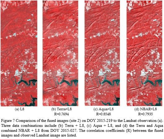
Figure 7 demonstrates data fusion examples produced from different data source combinations. Predictions for the DOY 219 in 2015 were generated based with STARFM one input image pair on DOY 2015-027 generated from three different data source combinations (Terra + L8, Aqua + L8, and the combined NBAR + L8) (the original NBAR images are shown in Figure 6D). Comparing to the direct Landsat observation from the same date, we can see the best predicted image comes from the combination of Aqua + L8 (the highest R), while the poorest one is from the combination of Terra + L8 due to a larger discrepancy in viewing geometries between these two sensors. The larger VZA results in a lower effective spatial resolution for Terra NBAR image (such as Figure 6D), and generates a fused image with lower fidelity (Figure 7b). Although the spatial resolution of the combined NBAR image is only 500 m, the effective spatial resolution of the Terra-Aqua combined NBAR products can be better than that of the Terra NBAR products. The fusion result from the NBAR + L8 image pair also shows clear surface features, with R near 0.8 in comparison with the direct Landsat observation.
4.3. Effect of Pair Date
Figure 5 shows that the annually averaged MAD between predicted and observed reflectance at Landsat scale varies with the input pair date and shows a seasonal variation. The errors may be partially due to the inconsistency between Landsat and MODIS data products. Figure 8 shows the MAD between the observed Landsat NDVI and the fused results at each Landsat overpass date using the simulated MODIS data, segregated by land cover type. In the MAD panels in this figure, the different color lines signify different pair dates used as fusion input to predict NDVI on different prediction dates (x axis). It can be seen that the predictability from a certain pair date varies with the prediction date. Generally, the closer the predicted date is to the pair date, the more accurate (smaller MAD) the prediction. Within a short time period (<50 days in our cases), the predictability decreases as the time interval between input and prediction date increases. For a long time period, phenology also plays a role in predictability. In Figure 8a, all pairs show poor predictions around the crop green-up and senescence times. This is likely due to the fact that crops are changing rapidly during these periods, and vegetation patterns are very different from patterns at other times during the year. Human management activities such as irrigation and harvest are also an impact factor. In the forest study area (site 2, Figure 8b), pair dates in the growing or non-growing season can be used to reasonably predict reflectance within the same season, but will less accurately predict reflectance in different seasons.
The temporally-averaged MAD (<MAD>) for each selected pair image is calculated by comparing data fusion results to Landsat observations from the entire year and is shown in Figure 9. For all vegetated land covers, <MAD> based on the pair dates from the growing season are relative larger than those from the non-growing season, partially due to the fact that the growing season is short and there are more validation images from the non-growing season, especially for agricultural site 1. For crop fields (corn and soybeans), the MAD function with prediction date has a characteristic “M” shape for most pair dates (Figure 8a); i.e., we obtain larger MAD during the green-up and senescence periods, but relatively smaller MAD in the non-growing seasons and at the time of peak growth. For forests, MAD patterns for different prediction dates are straightforward; i.e., pairs from the growing season have better prediction skill during the growing season than the non-growing season and vice versa (Figure 8b). Even though the year-long predictability for crops using a growing season image pair is poor, the pair images from the growing season have better predictability during the growing season or nearby dates.
The mean NDVI time series for corn and soybean pixels from the observed Landsat and the predicted images based on different pair dates (80, 224, and 283) are computed and extracted. The selected pair dates represent input images collected during an inactive date (DOY 80), a peak growing date (DOY 224) and a senescence date (DOY 263). Figure 10 shows the annual NDVI compared to the observed Landsat NDVI for corn and soybean. Both corn and soybean show good fusion results and NDVI temporal patterns similar to the original Landsat even though only one pair image was used in predicting an entire year. However, the predictability for different pair dates is slightly different, particularly for soybean. In that case, predictions using an image pair from the inactive season are slightly underestimated for the growing season, while those based on growing season pairs are mostly overestimated for the inactive season. A possible reason is that corn is a major crop in the study area (55% for corn and 35% for soybean) and MODIS temporal information mostly reflected corn growth conditions in the mixed MODIS pixels. Corn and soybeans have different growth patterns (see NDVI curves in Figure 8a). Corn is planted earlier and emerges earlier than soybeans. After reaching peak values, corn NDVI values become smaller than soybeans. The mixture of corn and soybeans at MODIS pixel resolution may cause errors when predicting Landsat images using image pairs from different seasons.
4.4. Effect of Land Cover Type
Figure 9 shows the temporally-averaged MAD (<MAD>) for five land covers. The <MAD> trends from the three forest classes are similar, where <MAD> for evergreen forest is the lowest, followed by deciduous forest, and then the mixed forest. The <MAD> for forest classes are all lower than the crop classes since the forest classes in this study have less temporal NDVI variation and lower peak NDVI than the crop classes. For crop fields, the prediction accuracy is better for corn than for soybeans, especially during the growing peak season. One of the reasons may be the different field sizes and planting areas for these two crops at study site 1. In fact, corn fields are typically larger than soybean fields in site 1. A larger field size means it is easier to find MODIS pure pixels and, thus, better predictions are obtained. Comparing with the forest land cover, crops have relatively larger MAD in this study. One of the reasons may be that cropped landscapes are more heterogeneous (see the discussion in Section 5.2). Additionally, crops change faster than forests due to the human management. One typical example for soybean and corn is shown in Figure 10. It can be found that the discrepancy between fused and original NDVI for corn is slightly smaller than that for soybean. One possible reason is that soybean during the growing season in the study area is shorter than corn so that its reflectance/NDVI change is faster than corn. According to the USDA crop progress statistics, soybeans at site 1 are generally planted 2–3 weeks later, and harvested about two weeks earlier than corn. This makes the seasonal evolution in reflectance harder to predict given a single input pair. Crop planting and harvesting are a kind of land cover change in the data fusion process. The spatial information from Landsat images during the non-growing season may not be applicable to the growing season, and vice versa.
4.5. Pair Selection Strategies
To test the two automatic pair selection strategies (ND and HC), image pairs on DOY 80 and DOY 263 were used to predict the entire year for site 1. Results show that the split day is 170 for the ND approach and 193 for the HC approach. Figure 11 shows the variation in MAD with the prediction date using these two pair selection strategies. Only results for prediction dates between the split days (170–193) differ based on strategy. During that period, the HC strategy yields lower <MAD> values, indicating superior performance in comparison with ND in this case.
While the tests portrayed in Figure 11 limit available pairs to two, Figure 12 explores the impact on <MAD> of increasing the number of pairs available to choose from. Except for the first point on the left (only one pair available and, thus, <MAD> for ND and HC are identical), <MAD> using HC is always smaller than one using ND. If two pairs with a very long lapse (e.g., 80–224 and 80–263) are used, the difference between the HC and ND strategies becomes larger. With increasing number of available image pairs, the MADs from both HC and ND decrease and the differences between the two strategies become smaller since the split dates decided by the ND and HC strategy are close. Generally, the HC strategy is superior to ND in this study. The HC strategy requires more time to compute the correlation coefficient between the predicted and pair date images. When there are only a small number of available image pairs during a long time interval, the HC strategy is a better choice. If there are a large number of image pairs and the pair dates are close, both HC and ND yield similar accuracy, while ND is a simple and fast method to decide the split dates operationally.
Figure 12 also reveals that the year-long predictability of each image pair is different. The overall prediction accuracy for a long period may drop if an image pair with low predictability is included. In our study, the <MAD> based on the pair on DOY 80 decreases (improves) when a pair image on DOY 263 is added (Figure 12). However, the overall <MAD> increases (worsens) when another pair from DOY 224 is added. Although DOY 224 is around the peak growing stage (close to maximum NDVI), the year-long predictability of this pair is the lowest among all (see maximum <MAD> for corn in Figure 9). The year-long predictability of pairs in certain growth stages (e.g., green-up and senescence) is usually poor (Figure 8). In order to achieve high prediction accuracy for a long period, the pair dates during green-up and senescence stages should be used, but only limited to predictions for nearby dates. In our study, the MAD can be kept under 0.01 for no more than 50 days around these pair dates.
5. Discussion
5.1. Selection of Data Sources
MODIS observations are subject to variations in view zenith angle. According to our results, the combinations of data sources with smaller VZA have the smaller RMSE and larger R between MODIS and Landsat (Figure 4) and produce the better predictions (Figure 5). Using six combinations of MODIS (Terra, Aqua, and combined) and Landsat (Landsat 7 and 8) images as data fusion sources, we find that daily MODIS observations with a smaller view zenith angle can produce better data fusion results. This can be taken as a rule to select appropriate MODIS image pairs. In fact, the VZAs of MODIS data on Landsat acquisition dates are basically similar for the same study area due to the same nadir revisit cycle (every 16 days). Therefore, pairs of Terra + L7 images usually work better as input to a fusion system than the other combinations, because both sensors are flying in formation and are viewing near-nadir on Landsat overpass dates. However, Landsat 7 has been suffering the failure of the SLC since May 2003. The combination of Terra + L7 is not very effective for data fusion especially at the edge of the Landsat scene. A remedy is to gap-fill the Landsat 7 ETM+ images before data fusion. Several gap filling methods have been developed in the past, such as the histogram matching approach, the Neighborhood Similar Pixel Interpolator (NSPI) and the Geostatistical Neighborhood Similar Pixel Interpolator (GNSPI) approach [35,44,45]. More efforts are needed to evaluate the usability of the gap-filled Landsat data. Other medium-resolution data, such as the Sentinel-2 Multispectral Instrument (MSI), with similar spectral bands to Landsat and MODIS, may be used as a data source to improve spatial-temporal data fusion.
For the Aqua + L8 combination, Aqua images are acquired around 1:30 P.M. local time and Landsat 8 are often acquired at ca. 11 A.M. Even though VZAs of Aqua MODIS are normally smaller at Landsat 8 overpass time than Terra MODIS, the different atmospheric conditions in the morning and afternoon may also introduce inconsistency.
The Collection 6 MODIS daily NBAR product is now available. It is generated using all clear sky directional reflectances over a 16-day period from both Aqua and Terra. Therefore, the combined NBAR product usually has more valid data than the contemporaneous daily Terra and Aqua MODIS image. The data quality of the Collection 6 NBAR product has been improved because more data are now used in inversion than in Collection 5, especially in the higher latitudes with high revisit frequency [27]. The mean RMSE and R for the combined NBAR used in data fusion are slightly lower than for our best combination of Terra/Aqua and Landsat. One reason is that the spatial resolution of the NBAR product (500 m) is lower than our in-house Terra and Aqua daily NBAR (250 m) in the red and NIR bands. It is reasonable to try Terra or Aqua MODIS with small VZA in data fusion first. If Aqua or Terra MODIS at 250 m resolution with small VZA is not available, or daily Terra/Aqua MODIS NBAR cannot be produced in-house, the Collection 6 MODIS daily NBAR product would be a good choice for data fusion.
In this study, we pay more attention to the solar-viewing characteristics of MODIS, while directional reflectance effects in Landsat data are ignored due to the narrow field of view (15°) and the small view zenith angle (≤7.5°). Roy et al. found that the variations of solar-viewing geometry over the year can cause apparent changes in reflectance even if the surface properties remain constant [25]. Therefore, they developed a general approach to producing Landsat NBAR for a nadir view and fixed solar zenith geometry. In the future, the Landsat NBAR data can be used instead of Landsat directional reflectance in data fusion experiments, which may improve the consistency of Landsat and MODIS NBAR images. Findings reported here based on different data source combinations are applicable to other spatial-temporal data fusion models that rely on Landsat-MODIS image pairs.
5.2. The Impact of Temporal and Spatial Variations on Prediction Accuracy
Complex heterogeneous areas with high temporal and spatial variations in surface reflectance may have lower prediction accuracies than more homogeneous areas [46]. This may be caused by several factors. First, vegetation in different climate regions has different temporal growing patterns. In our cases, the forest in site 2 has a longer growing season and shows less temporal variation in reflectance and NDVI than crops in site 1. The mean NDVI ranges from 0.5 to 0.8 for deciduous forest, and from 0.7–0.8 for evergreen forest. In comparison, the range of the mean NDVI for crops, both corn and soybean, is from ~0.2 to ~0.9 (Figure 8). Additionally, the growing period from green-up to senescence for crops in site 1 is about 140 days, while for forest in site 2 it is about 200 days. It is more difficult to capture the rapid changes in reflectance associated with the crop land classes, especially during the green-up and senescence stages (Figure 9).
Second, the accuracy of data fusion is also affected by the spatial heterogeneity within the study area. For example, land cover in site 2 is more homogenous than in site 1 during the growing season. There are large continuous patches of forest at site 2. Forests (deciduous, evergreen and mixed forests) in the area have similar NDVI during the growing season. Although over 90% of land covers at site 1 are crops, the spatial heterogeneity caused by the different crops and planting schedules is observed. Data fusion accuracy for forests is slightly higher than for croplands in these tests.
To assess the relative spatial variability for each study site, the mean squared displacement (MSD; Equation (5)) was computed for each Landsat image and plotted in Figure 13. Again, MSD represents the spatial heterogeneity of land cover in reflectance or NDVI. It can be seen that MSD is smallest for red reflectance, followed by NIR and NDVI. As the crops grow, the spatial variability in NIR first increases, and then decreases (opposite for the red band). The MSD for NDVI varies greatly over the course of the year, and attains high values indicating large spatial variability. Near peak growth, however, the NDVI of corn and soybean is more similar and the landscape at site 1 appears more homogeneous; therefore, NDVI MSD decreases during this period. When the NDVI MSD reaches a maximum during the green-up and senescent stages, the different seeding/harvest schedules and different growth rates of various crop types lead to rapid changes in the image texture causing stronger spatial heterogeneity. The prediction accuracies during these two periods are lower than for other stages.
For site 2, reflectances in the red and NIR bands are relative stable during the entire growing season. Unlike crops, the MSD for forest in the non-growing season is slightly higher than in the growing season, which means that forests are more homogeneous during the growing season. Therefore, the data fusion accuracies from forests are normally higher than for crops, as illustrated in Figure 9.
5.3. Pair Selection Strategies
Additional image pairs available during a time period can improve data fusion results, especially when some key pair dates (e.g., the green-up and senescence stages for crops) are available. This implies that with a few key pairs of input we may be able to produce high quality data fusion results for a long time-series. However, in many areas and applications, we do not have control over the numbers and dates of clear image pairs. For the study sites analyzed here, after three pairs of Landsat and MODIS images are used, the improvement of the <MAD> is not very obvious (Figure 12). This is likely not the case for fusion of images depicting quantities that change more rapidly than surface reflectance, such as evapotranspiration. This observation is also specific to the cropping system investigated here. Double cropping systems or crops with multiple harvests per season (e.g., alfalfa) will likely require more input image pairs to successfully predict the full growing season with adequate accuracy.
The year-long predictability of an image pair depends on the pair date. Pairs from periods of rapid change have lower long-term predictive skill even though they are good for nearby dates. These pairs should be included, but limited to nearby prediction dates. Additionally, the optimal image pair may be related to the spatial texture in Landsat images. For example, a base image pair from spring may have similar spatial texture to that from autumn. The prediction for autumn images using a spring image pair may work better than using a summer image. Since we do not know the texture change at the Landsat scale on the prediction date, additional information beyond the Landsat and MODIS images will be needed to decide the optimal pair to use. This information could be related to the crop growth calendar, historical vegetation phenology from past years, or observations from the ground. A key is to select the pair that can best describe the spatial variation on the prediction date. If land covers were stable in the past years, the image pair from previous years within the same season may be used [15]. However, this could be a problem in areas like site 1, where corn and soybean crops are generally rotated on an annual basis.
6. Conclusions
The accuracy of spatial-temporal data fusion results depends on both the data fusion model and input data used in the fusion process. In order to give guidance for choosing the optimal image pairs, this paper evaluates the accuracy of fusing data from different combinations of MODIS-Landsat data sources using the STARFM data fusion model as an example. The predictive skill of different pair images is assessed in terms of input data consistency, vegetation phenology, and land cover types for two vegetated areas including crops and forests. The results show that MODIS images with smaller view zenith angle always produce better fusion results. The combination of Terra NBAR and Landsat 7 produces better results than other combinations in red and NIR wavebands. However, SLC-off gaps in Landsat 7 ETM+ image limit data fusion application. The combination of Aqua NBAR and Landsat 8 is also a good option. Since the Terra or Aqua daily NBAR at 250 m resolution needs to be produced in-house, the standard collection six MODIS daily NBAR products at 500 m resolution can be ordered directly and will be good for operational uses. This conclusion is drawn based on the analysis of the Landsat-MODIS image pairs and, thus, can be applied to other spatial-temporal data fusion models.
Data fusion results are affected by the selection of image pairs and by different land covers. The prediction accuracy for forests is higher than crops in our study areas. Generally, pairs from the growing season have a better predictability during the growing season than the non-growing season and vice versa. With the increase of the time interval between pair and predicted dates, the pair predictability will decrease. While the prediction accuracy based on the non-growing season pairs decreases more slowly than that based on the growing season pairs due to rapid changes in the vegetation on the land surface during the growing season. Especially, the derived NDVI from the fused surface reflectance are overestimated for the non-growing seasons when using the growing season image pair, and underestimated for the growing season slightly when using the non-growing season pairs. Data fusion accuracy can be improved if some key image pairs during different vegetation phenology stages are included. The evaluation on the two automatic pair selection strategies (the nearest date, ND, and higher correlation, HC) reveals that the HC strategy works better than the ND strategy. With the increase of image pairs, the difference between two strategies decreases. In general, our results show that the spatial-temporal data fusion can be improved by choosing suitable image pairs.
Author Contributions
D.X. processed the data and prepared the draft; F.G. helped fuse the remote sensing data and modify the STARFM program; and both L.S. and M.A. helped analyze the results. All authors contributed to paper revisions.
Acknowledgments
This work was partially supported by the National Natural Science Foundation of China (grant nos. 41571341 and 41331171), the NASA Science of Terra, Aqua and Suomi NPP program, the NASA LCLUC program, and the US Geological Survey (USGS) Landsat Science Team program. USDA is an equal opportunity provider and employer.
Conflicts of Interest
The authors declare no conflict of interest.
References
- Woodcock, C.E.; Strahler, A.H. The factor of scale in remote sensing. Remote Sens. Environ. 1987, 21, 311–332. [Google Scholar] [CrossRef]
- Pax-Lenney, M.; Woodcock, C.E. The effect of spatial resolution on the ability to monitor the status of agricultural lands. Remote Sens. Environ. 1997, 61, 210–220. [Google Scholar] [CrossRef]
- Roy, D.P.; Wulder, M.A.; Loveland, T.R.; Woodcock, C.E.; Allen, R.G.; Anderson, M.C.; Helder, D.; Irons, J.R.; Johnson, D.M.; Kennedy, R.; et al. Landsat-8: Science and product vision for terrestrial global change research. Remote Sens. Environ. 2014, 145, 154–172. [Google Scholar] [CrossRef]
- Giri, C.; Pengra, B.; Long, J.; Loveland, T.R. Next generation of global land cover characterization, mapping, and monitoring. Int. J. Appl. Earth Obs. Geoinf. 2013, 25, 30–37. [Google Scholar] [CrossRef]
- Giambene, G. Resource Management in Satellite Networks: Optimization and Cross-Layer Design; Springer: New York, NY, USA, 2007. [Google Scholar]
- Gao, F.; Masek, J.; Schwaller, M.; Hall, F. On the blending of the Landsat and MODIS surface reflectance: Predicting daily Landsat surface reflectance. IEEE Trans. Geosci. Remote Sens. 2006, 44, 2207–2218. [Google Scholar]
- Zhukov, B.; Oertel, D.; Lanzl, F.; Reinhackel, G. Unmixing-based multisensor multiresolution image fusion. IEEE Trans. Geosci. Remote Sens. 1999, 37, 1212–1226. [Google Scholar] [CrossRef]
- Song, H.; Huang, B. Spatiotemporal Satellite Image Fusion through One-Pair Image Learning. IEEE Trans. Geosci. Remote Sens. 2013, 51, 1883–1896. [Google Scholar] [CrossRef]
- Zhu, X.; Helmer, E.H.; Gao, F.; Liu, D.; Chen, J.; Lefsky, M.A. A flexible spatiotemporal method for fusing satellite images with different resolutions. Remote Sens. Environ. 2016, 172, 165–177. [Google Scholar] [CrossRef]
- Zhu, X.; Cai, F.; Tian, J.; Williams, T. Spatiotemporal Fusion of Multisource Remote Sensing Data: Literature Survey, Taxonomy, Principles, Applications, and Future Directions. Remote Sens. 2018, 10, 527. [Google Scholar] [CrossRef]
- Hilker, T.; Wulder, M.A.; Coops, N.C.; Linke, J.; McDermid, G.; Masek, J.G.; Gao, F.; White, J.C. A new data fusion model for high spatial- and temporal-resolution mapping of forest disturbance based on Landsat and MODIS. Remote Sens. Environ. 2009, 113, 1613–1627. [Google Scholar] [CrossRef]
- Fu, D.; Chen, B.; Wang, J.; Zhu, X.; Hilker, T. An Improved Image Fusion Approach Based on Enhanced Spatial and Temporal the Adaptive Reflectance Fusion Model. Remote Sens. 2013, 5, 6346–6360. [Google Scholar] [CrossRef] [Green Version]
- Gevaert, C.M.; García-Haro, F.J. A comparison of STARFM and an unmixing-based algorithm for Landsat and MODIS data fusion. Remote Sens. Environ. 2015, 156, 34–44. [Google Scholar] [CrossRef]
- Shen, H.; Wu, P.; Liu, Y.; Ai, T.; Wang, Y.; Liu, X. A spatial and temporal reflectance fusion model considering sensor observation differences. Int. J. Remote Sens. 2013, 34, 4367–4383. [Google Scholar] [CrossRef]
- Wang, P.; Gao, F.; Masek, J.G. Operational Data Fusion Framework for Building Frequent Landsat-Like Imagery. IEEE Trans. Geosci. Remote Sens. 2014, 52, 7353–7365. [Google Scholar] [CrossRef]
- Frantz, D.; Röder, A.; Udelhoven, T.; Schmidt, M. Forest Disturbance Mapping Using Dense Synthetic Landsat/MODIS Time-Series and Permutation-Based Disturbance Index Detection. Remote Sens. 2016, 8, 277. [Google Scholar] [CrossRef]
- Walker, J.J.; de Beurs, K.M.; Wynne, R.H.; Gao, F. Evaluation of Landsat and MODIS data fusion products for analysis of dryland forest phenology. Remote Sens. Environ. 2012, 117, 381–393. [Google Scholar] [CrossRef]
- Senf, C.; Leitão, P.J.; Pflugmacher, D.; van der Linden, S.; Hostert, P. Mapping land cover in complex Mediterranean landscapes using Landsat: Improved classification accuracies from integrating multi-seasonal and synthetic imagery. Remote Sens. Environ. 2005, 156, 527–536. [Google Scholar] [CrossRef]
- Singh, D. Generation and evaluation of gross primary productivity using Landsat data through blending with MODIS data. Int. J. Appl. Earth Obs. Geoinf. 2011, 13, 59–69. [Google Scholar] [CrossRef]
- Semmens, K.A.; Anderson, M.C.; Kustas, W.P.; Gao, F.; Alfieri, J.G.; McKee, L.; Prueger, J.H.; Hain, C.R.; Cammalleri, C.; Yang, Y.; et al. Monitoring daily evapotranspiration over two California vineyards using Landsat 8 in a multi-sensor data fusion approach. Remote Sens. Environ. 2016, 185, 155–170. [Google Scholar] [CrossRef] [Green Version]
- Dong, T.; Liu, J.; Qian, B.; Zhao, T.; Jing, Q.; Geng, X.; Wang, J.; Huffman, T.; Shang, J. Estimating winter wheat biomass by assimilating leaf area index derived from fusion of Landsat-8 and MODIS data. Int. J. Appl. Earth Obs. Geoinf. 2016, 49, 63–74. [Google Scholar] [CrossRef]
- Emelyanova, I.V.; McVicar, T.R.; van Niel, T.G.; Li, L.T.; van Dijk, A.I.J.M. Assessing the accuracy of blending Landsat–MODIS surface reflectances in two landscapes with contrasting spatial and temporal dynamics: A framework for algorithm selection. Remote Sens. Environ. 2013, 133, 193–209. [Google Scholar] [CrossRef]
- Gao, F.; Anderson, M.C.; Zhang, X.; Yang, Z.; Alfieri, J.G.; Kustas, W.P.; Mueller, R.; Johnson, D.M.; Prueger, J.H. Toward mapping crop progress at field scales through fusion of Landsat and MODIS imagery. Remote Sens. Environ. 2017, 188, 9–25. [Google Scholar] [CrossRef]
- Gao, F.; He, T.; Masek, J.G.; Shuai, Y.; Schaaf, C.B.; Wang, Z. Angular Effects and Correction for Medium Resolution Sensors to Support Crop Monitoring. IEEE J. Sel. Top. Appl. Earth Obs. Remote Sens. 2014, 7, 4480–4489. [Google Scholar] [CrossRef]
- Roy, D.P.; Zhang, H.K.; Ju, J.; Gomez-Dans, J.L.; Lewis, P.E.; Schaaf, C.B.; Sun, Q.; Li, J.; Huang, H.; Kovalskyy, V. A general method to normalize Landsat reflectance data to nadir BRDF adjusted reflectance. Remote Sens. Environ. 2016, 176, 255–271. [Google Scholar] [CrossRef]
- Schaaf, C.B.; Gao, F.; Strahler, A.H.; Lucht, W.; Li, X.; Tsang, T.; Strugnell, N.C.; Zhang, X.; Jin, Y.; Muller, J.-P.; et al. First operational BRDF, albedo nadir reflectance products from MODIS. Remote Sens. Environ. 2002, 83, 135–148. [Google Scholar] [CrossRef] [Green Version]
- Wang, Z.; Schaaf, C.B.; Sun, Q.; Shuai, Y.; Román, M.O. Capturing rapid land surface dynamics with Collection V006 MODIS BRDF/NBAR/Albedo (MCD43) products. Remote Sens. Environ. 2018, 207, 50–64. [Google Scholar] [CrossRef]
- Campagnolo, M.L.; Sun, Q.; Liu, Y.; Schaaf, C.; Wang, Z.; Román, M.O. Estimating the effective spatial resolution of the operational BRDF, albedo, and nadir reflectance products from MODIS and VIIRS. Remote Sens. Environ. 2016, 175, 52–64. [Google Scholar] [CrossRef]
- Zhu, X.; Chen, J.; Gao, F.; Chen, X.; Masek, J.G. An enhanced spatial and temporal adaptive reflectance fusion model for complex heterogeneous regions. Remote Sens. Environ. 2010, 114, 2610–2623. [Google Scholar] [CrossRef]
- Olexa, E.M.; Lawrence, R.L. Performance and effects of land cover type on synthetic surface reflectance data and NDVI estimates for assessment and monitoring of semi-arid rangeland. Int. J. Appl. Earth Obs. Geoinf. 2014, 30, 30–41. [Google Scholar] [CrossRef]
- Boryan, C.; Yang, Z.; Mueller, R.; Craig, M. Monitoring US agriculture: The US Department of Agriculture, National Agricultural Statistics Service, Cropland Data Layer Program. Geocarto Int. 2011, 26, 341–358. [Google Scholar] [CrossRef]
- MODIS Data Products, 2015. Downloaded from http://reverb.echo.nasa.gov/ (accessed on 23 December 2016).
- Friedl, M.A.; Sulla-Menashe, D.; Tan, B.; Schneider, A.; Ramankutty, N.; Sibley, A.; Huang, X. MODIS Collection 5 global land cover: Algorithm refinements and characterization of new datasets. Remote Sens. Environ. 2010, 114, 168–182. [Google Scholar] [CrossRef]
- Gao, F.; Masek, J.G.; Wolfe, R.E.; Huang, C. Building a consistent medium resolution satellite data set using moderate resolution imaging spectroradiometer products as reference. J. Appl. Remote Sens. 2010, 4, 43526. [Google Scholar]
- Landsat Surface Reflectance Products, 2015. Downloaded from http://earthexplorer.usgs.gov/ (accessed on 23 December 2016).
- Zhu, X.; Liu, D.; Chen, J. A new geostatistical approach for filling gaps in Landsat ETM+ SLC-off images. Remote Sens. Environ. 2012, 124, 49–60. [Google Scholar] [CrossRef]
- Masek, J.G.; Vermote, E.F.; Saleous, N.E.; Wolfe, R.; Hall, F.G.; Huemmrich, K.F.; Gao, F.; Kutler, J.; Lim, T.-K. A Landsat Surface Reflectance Dataset for North America, 1990–2000. IEEE Geosci. Remote Sens. Lett. 2006, 3, 68–72. [Google Scholar] [CrossRef]
- Vermote, E.; Justice, C.; Claverie, M.; Franch, B. Preliminary analysis of the performance of the Landsat 8/OLI land surface reflectance product. Remote Sens. Environ. 2016, 185, 46–56. [Google Scholar] [CrossRef]
- USDA Cropland Data Layer (CDL), 2015. Downloaded from https://nassgeodata.gmu.edu/CropScape/ (accessed on 23 December 2016).
- Hilker, T.; Wulder, M.A.; Coops, N.C.; Seitz, N.; White, J.C.; Gao, F.; Masek, J.G.; Stenhouse, G. Generation of dense time series synthetic Landsat data through data blending with MODIS using a spatial and temporal adaptive reflectance fusion model. Remote Sens. Environ. 2009, 113, 1988–1999. [Google Scholar] [CrossRef]
- Huang, C.; Townshend, J.R.G.; Liang, S.; Kalluri, S.N.V.; DeFries, R.S. Impact of sensor’s point spread function on land cover characterization: Assessment and deconvolution. Remote Sens. Environ. 2002, 80, 203–212. [Google Scholar] [CrossRef]
- Tan, B.; Woodcock, C.E.; Hu, J.; Zhang, P.; Ozdogan, M.; Huang, D.; Yang, W.; Knyazikhin, Y.; Myneni, R.B. The impact of gridding artifacts on the local spatial properties of MODIS data: Implications for validation, compositing, and band-to-band registration across resolutions. Remote Sens. Environ. 2006, 105, 98–114. [Google Scholar] [CrossRef]
- Roy, D.P.; Ju, J.; Lewis, P.; Schaaf, C.; Gao, F.; Hansen, M.; Lindquist, E. Multi-temporal MODIS–Landsat data fusion for relative radiometric normalization, gap filling, and prediction of Landsat data. Remote Sens. Environ. 2008, 112, 3112–3130. [Google Scholar] [CrossRef]
- Chen, J.; Zhu, X.; Vogelmann, J.E.; Gao, F.; Jin, S. A simple and effective method for filling gaps in Landsat ETM+ SLC-off images. Remote Sens. Environ. 2011, 115, 1053–1064. [Google Scholar] [CrossRef]
- Romero-Sanchez, M.E.; Ponce-Hernandez, R.; Franklin, S.E.; Aguirre-Salado, C.A. Comparison of data gap-filling methods for Landsat ETM+ SLC-off imagery for monitoring forest degradation in a semi-deciduous tropical forest in Mexico. Int. J. Remote Sens. 2015, 36, 2786–2799. [Google Scholar] [CrossRef]
- Jarihani, A.; McVicar, T.; van Niel, T.; Emelyanova, I.; Callow, J.; Johansen, K. Blending Landsat and MODIS Data to Generate Multispectral Indices: A Comparison of ‘Index-then-Blend’ and ‘Blend-then-Index’ Approaches. Remote Sens. 2014, 6, 9213–9238. [Google Scholar] [CrossRef] [Green Version]
Figure 1.
Experimental sites and the boundaries of the Landsat scenes (a) with corresponding land cover maps from the Cropland Data Layer for 2015 (b).
Figure 1.
Experimental sites and the boundaries of the Landsat scenes (a) with corresponding land cover maps from the Cropland Data Layer for 2015 (b).

Figure 2.
Cloud-free Landsat 7 (green dots) and 8 (red dots) images from 2015 were used in the study. Landsat 8 images from p28r31 and p29r31 were used as pair images while Landsat 7 images were used to validate data fusion results in study site 1. Both Landsat 7 and 8 images for p25r36 can be used as pair images since Landsat 7 ETM+ images in study site 2 are not affected by the SLC-off problem. All validations only used Landsat images that were not used as input pair images.

Figure 3.
Schematic diagram for the nearest date (ND) and higher correlation (HC) pair selection strategies. The black line and red line represent Pearson correlation coefficient (R) values between MODIS images at pair base dates t1 and t2, respectively, and the prediction dates. R generally decrease with increasing MODIS image time separation. tm and tn are the split dates determined by the HC and ND strategies, individually.

Figure 4.
Temporally-averaged RMSE (<RMSE>) (a) and R (<R>) (b) for different combinations of MODIS and Landsat pair images for site 2. NBAR, Terra, and Aqua in the x axis represent the combinations of the Terra and Aqua combined NBAR, Terra NBAR, and Aqua NBAR with Landsat, respectively. Labels in the plot show the combinations of MODIS (NBAR, Terra, Aqua) and Landsat (L7 and L8) image pairs.

Figure 5.
Temporally-averaged mean absolute difference (<MAD>) for different combinations of pair images from MODIS (Terra, Aqua, and combined NBAR) and Landsat (Landsat 7 and 8) for site 1 (a) and site 2 (b). In site 1, <MAD> is calculated based on the predicted image from Landsat 8 (p28r31) in order to compare different pair combinations consistently.

Figure 6.
Comparison of the composite NBAR images from Terra (250 m), Aqua (250 m), and the combined products (500 m) with Landsat image for site 1 (A,B) and site 2 (C,D) from different Landsat dates. The images are composited using NIR, red and red bands as RGB (only red and NIR bands are available at 250 m resolution). The images for each date are linearly stretched using the same stretch range for better visualization. The view zenith angles (VZA) for Terra and Aqua images are the averaged VZAs from original directional reflectance. The figure shows that even after BRDF correction, the image quality and spatial detail in the MODIS data used as fusion inputs can vary significantly.


Figure 7.
Comparison of fused images (site 2) on DOY 2015-219 to the direct Landsat observation on that date (a). Three data combinations used in the fusion include (b) Terra + L8, (c) Aqua + L8, and (d) the Terra and Aqua combined NBAR + L8 from DOY 2015-027. The correlation coefficients (R) between the fused images and observed Landsat image are listed.

Figure 8.
Comparison of MAD between observed and predicted Landsat-scale NDVI for different prediction dates (x-axis) using different input pair dates (signified by different color lines) for crops at site 1 (a) and forest types at site 2 (b). Mean NDVI from vegetation land cover types (corn and soybean in site 1, and deciduous, evergreen and mixed forests in site 2) were extracted and averaged based on observed Landsat and CDL data. Each symbol represents the MAD between the observed Landsat (not used in data fusion) and the fused result. Four pair dates, including days 80 (non-growing season), 167 (around green-up dates), 224 (around peak growing dates), and 279 (around senescence) are highlighted (enlarged dots) for site 1. Two pair dates, including day 43 from the non-growing season and day 195 from the growing season are highlighted (enlarged dots) for site 2.

Figure 9.
Comparison of <MAD> (a) and <R> (b) as a function of pair date for different land cover types from both study sites (the results of corn and soybean are from site 1 and those of forests are from site 2).
Figure 9.
Comparison of <MAD> (a) and <R> (b) as a function of pair date for different land cover types from both study sites (the results of corn and soybean are from site 1 and those of forests are from site 2).

Figure 10.
Comparison of NDVI time series for corn (a) and soybean (b) from original Landsat observations (black) and the fused images using pair images on day 80 (red), 224 (green), and 283 (blue) for site 1.
Figure 10.
Comparison of NDVI time series for corn (a) and soybean (b) from original Landsat observations (black) and the fused images using pair images on day 80 (red), 224 (green), and 283 (blue) for site 1.

Figure 11.
MAD for different prediction dates based on one image pair option from either day 80 or 263 when using the nearest date (ND) and higher correlation (HC) strategies. The HC strategy shows the smaller MAD (red) and better data fusion results than the ND strategy (black).
Figure 11.
MAD for different prediction dates based on one image pair option from either day 80 or 263 when using the nearest date (ND) and higher correlation (HC) strategies. The HC strategy shows the smaller MAD (red) and better data fusion results than the ND strategy (black).

Figure 12.
<MAD> of NDVI decreases as the available number of pair images increases for both the ND and HC pair selection strategy. Each point in the plot shows a combination of pair dates, as indicated by the adjacent label.
Figure 12.
<MAD> of NDVI decreases as the available number of pair images increases for both the ND and HC pair selection strategy. Each point in the plot shows a combination of pair dates, as indicated by the adjacent label.

Figure 13.
MSD of Landsat reflectance (red and NIR) and NDVI for site 1 (a) and site 2 (b). A higher MSD means a more heterogeneous landscape.
Figure 13.
MSD of Landsat reflectance (red and NIR) and NDVI for site 1 (a) and site 2 (b). A higher MSD means a more heterogeneous landscape.


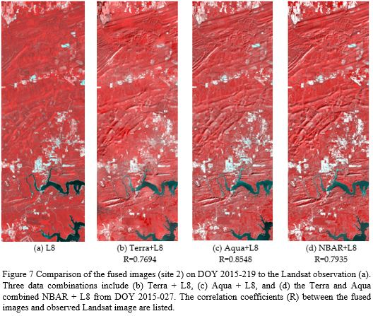
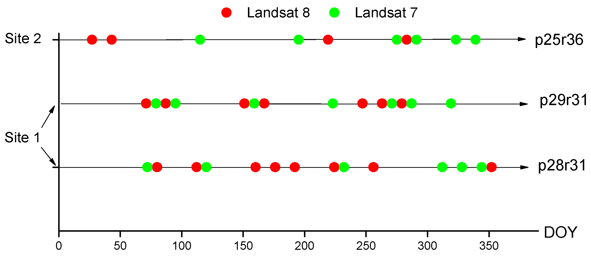
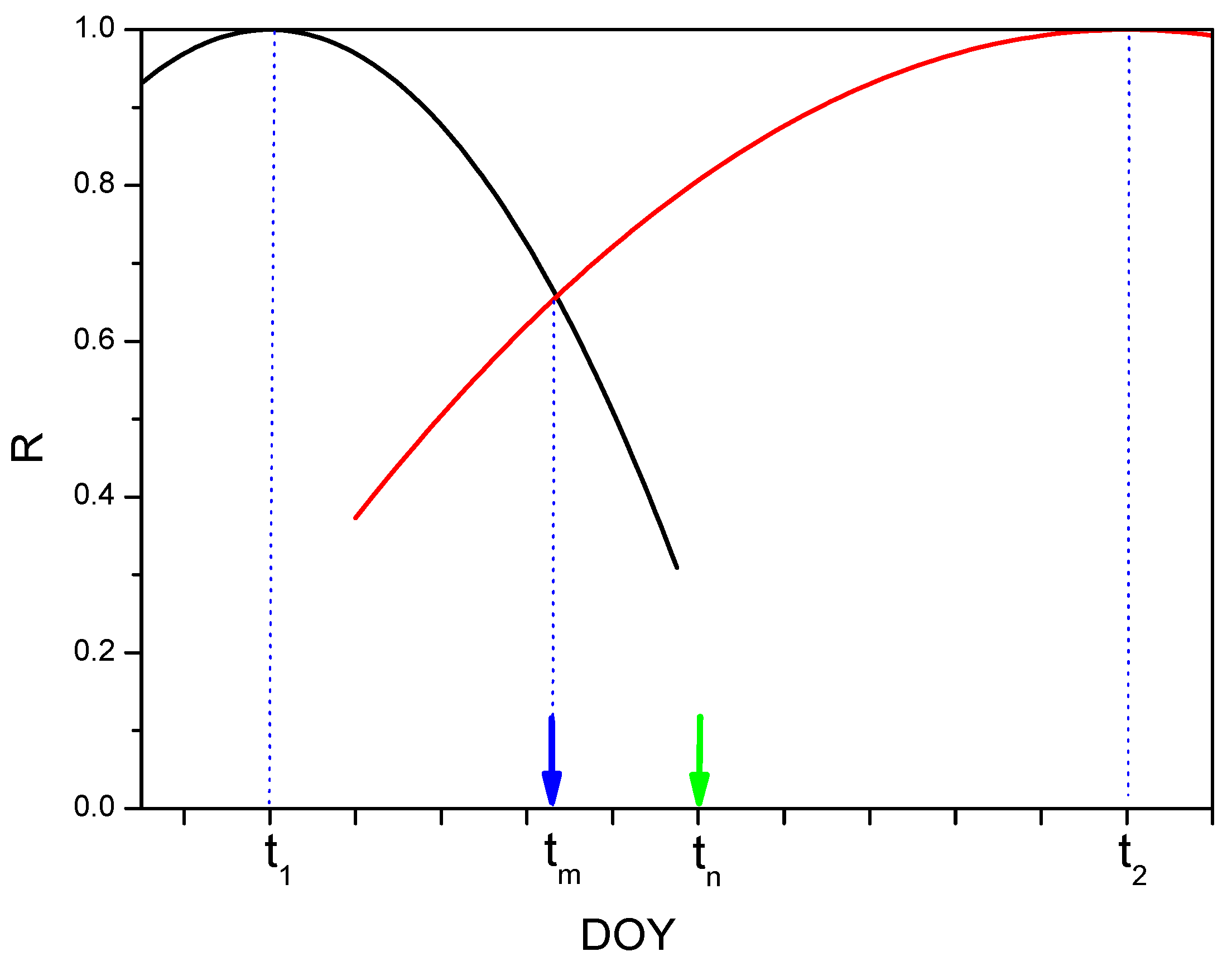
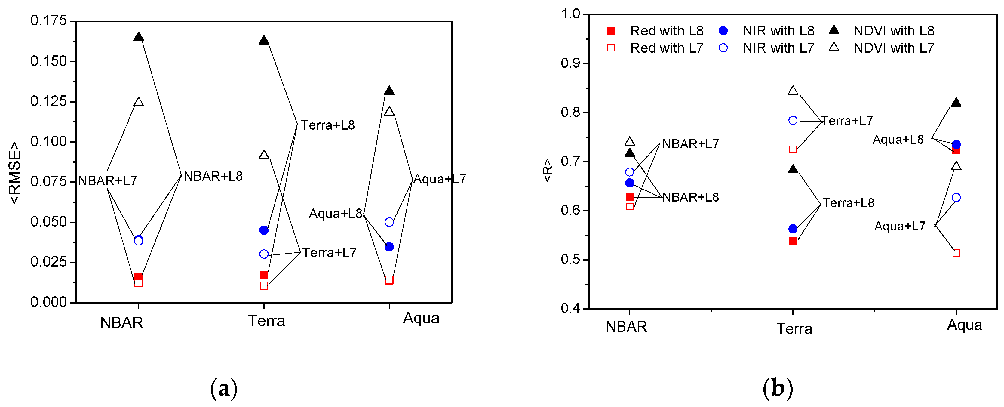
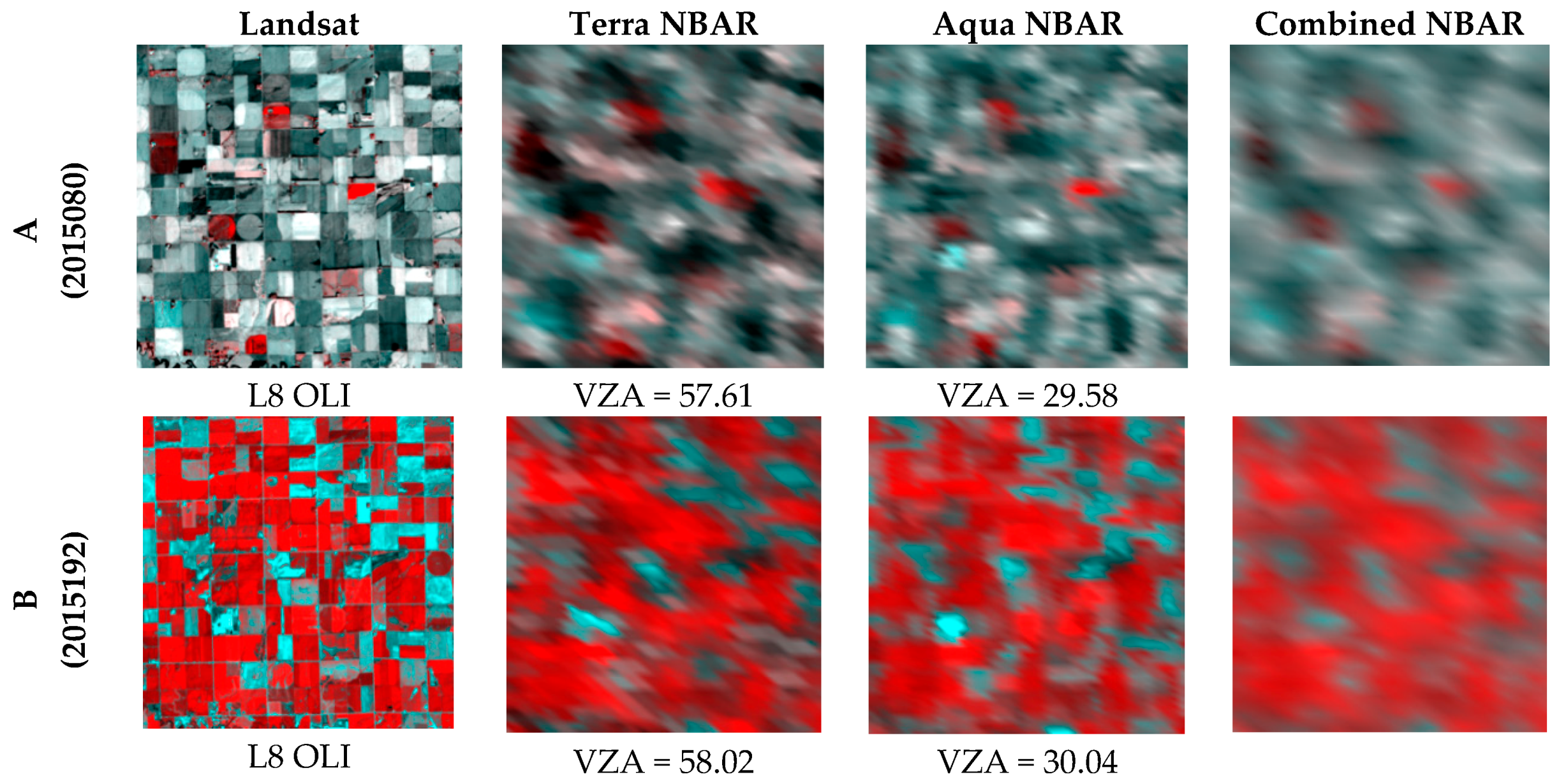
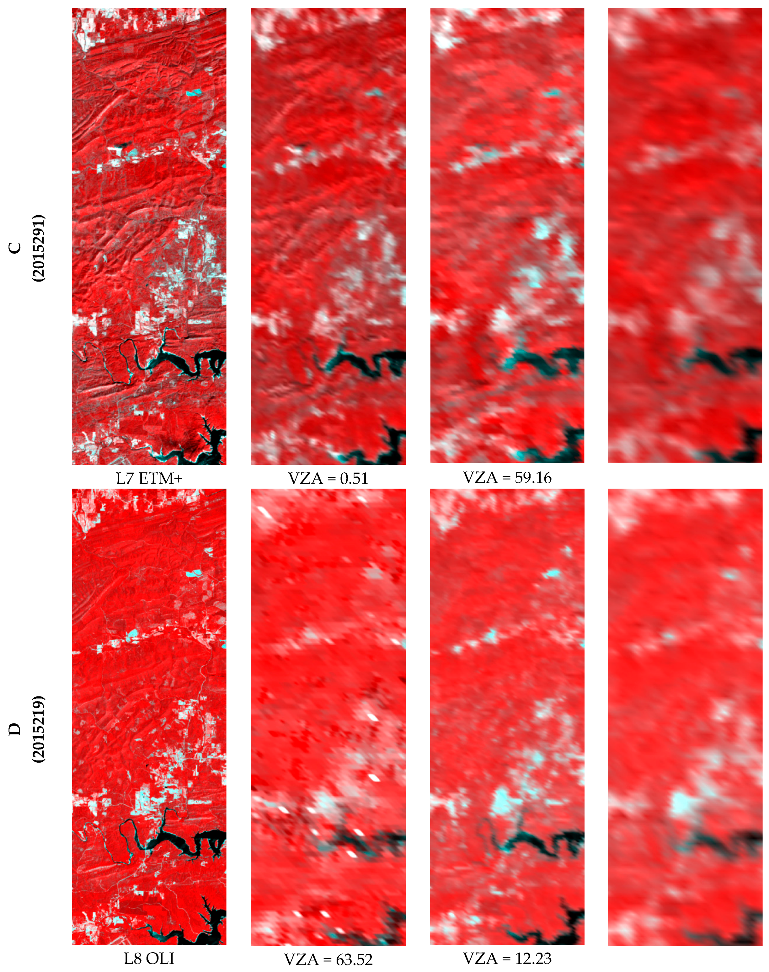
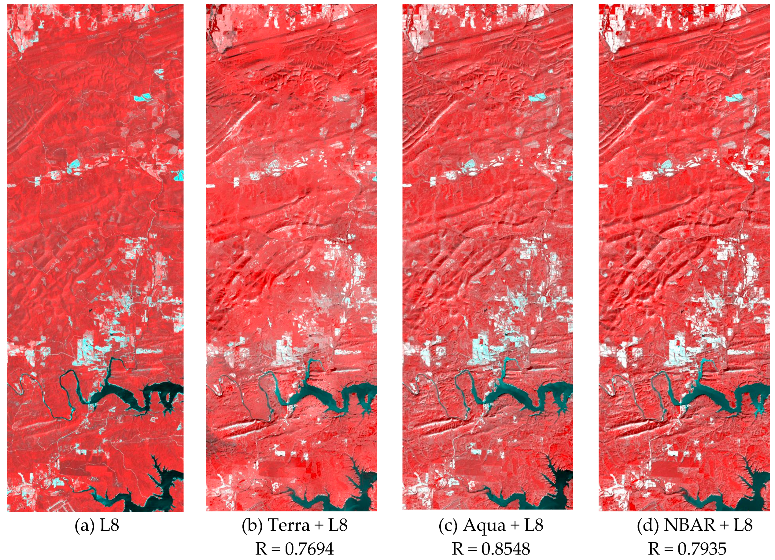
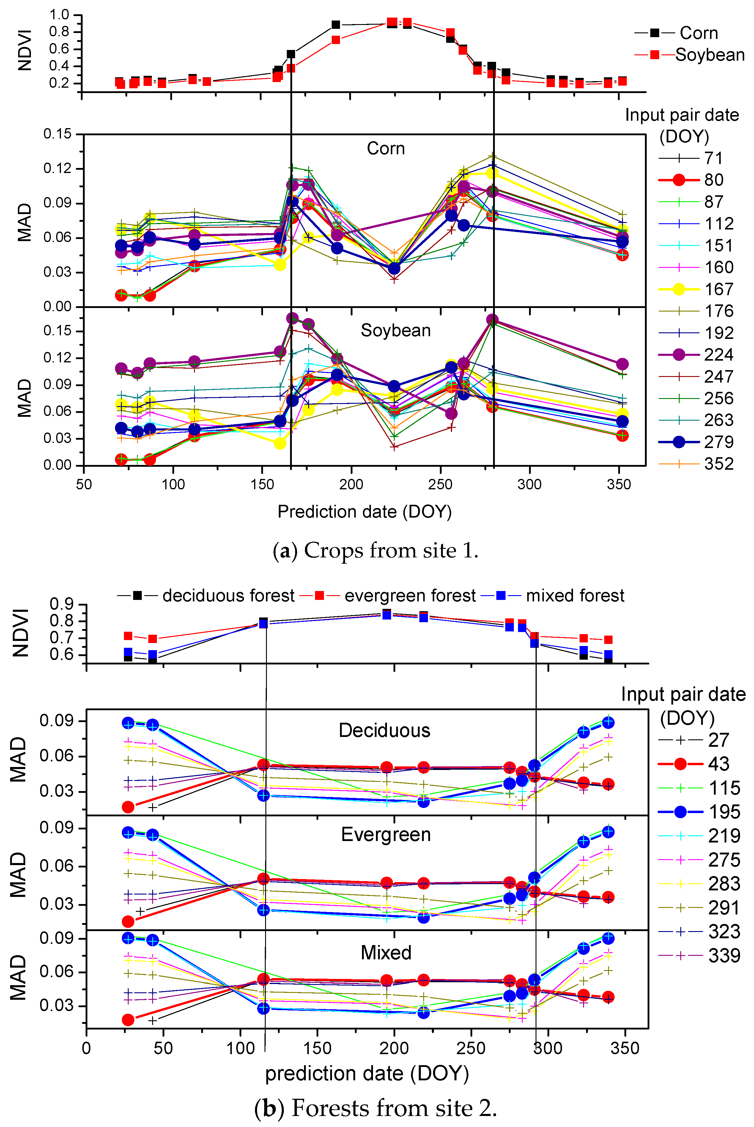
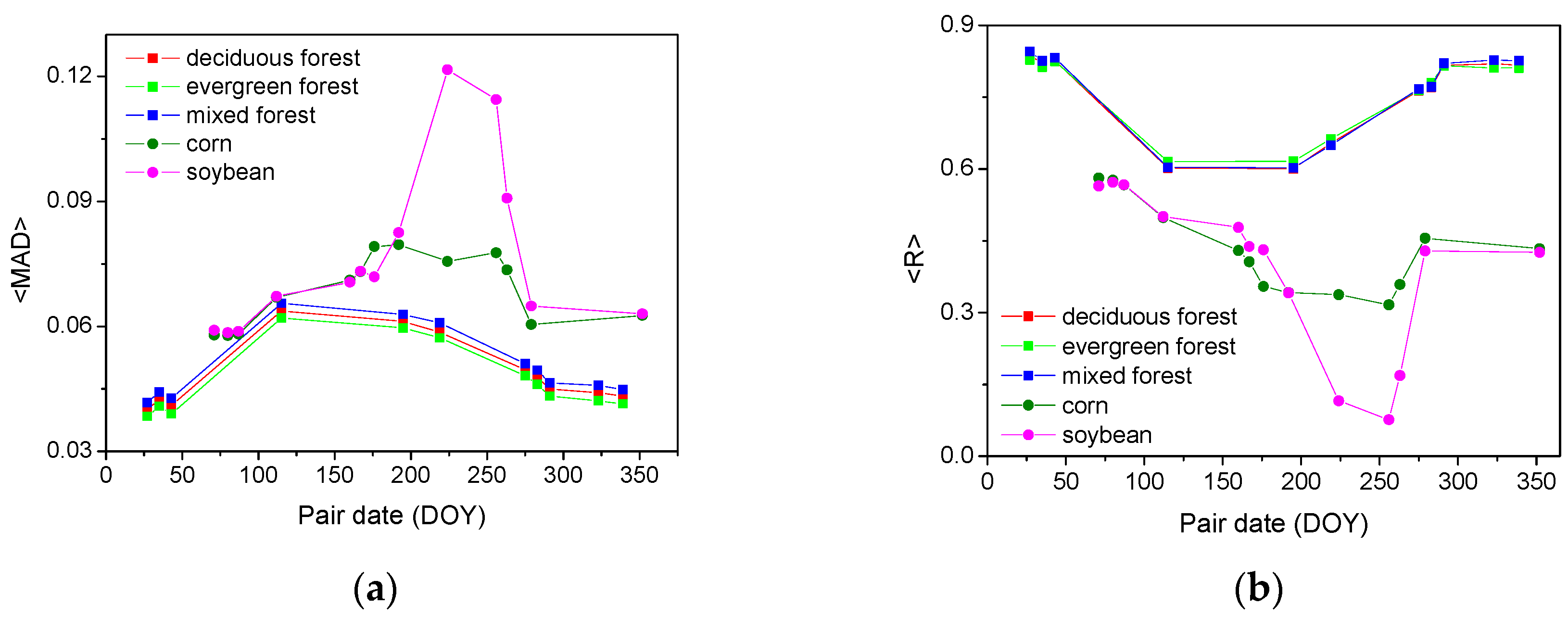
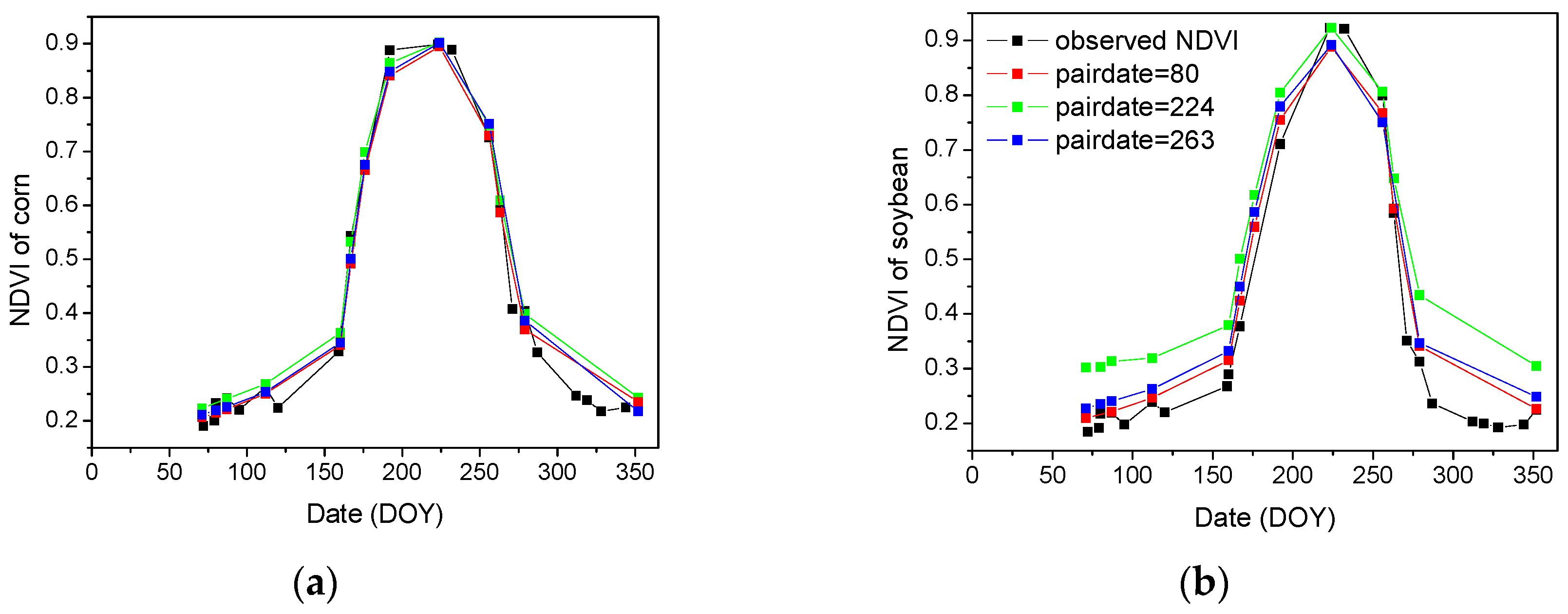
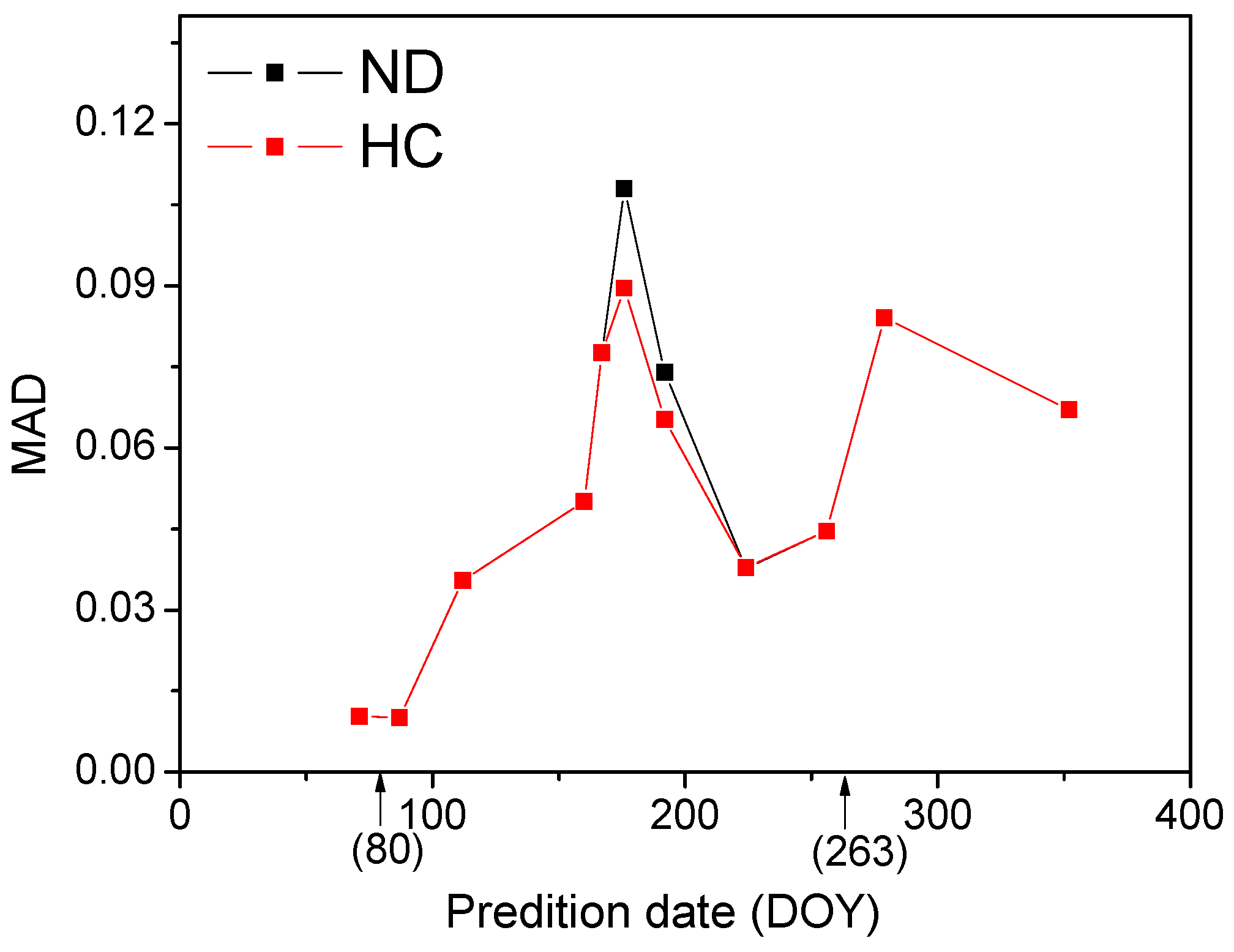
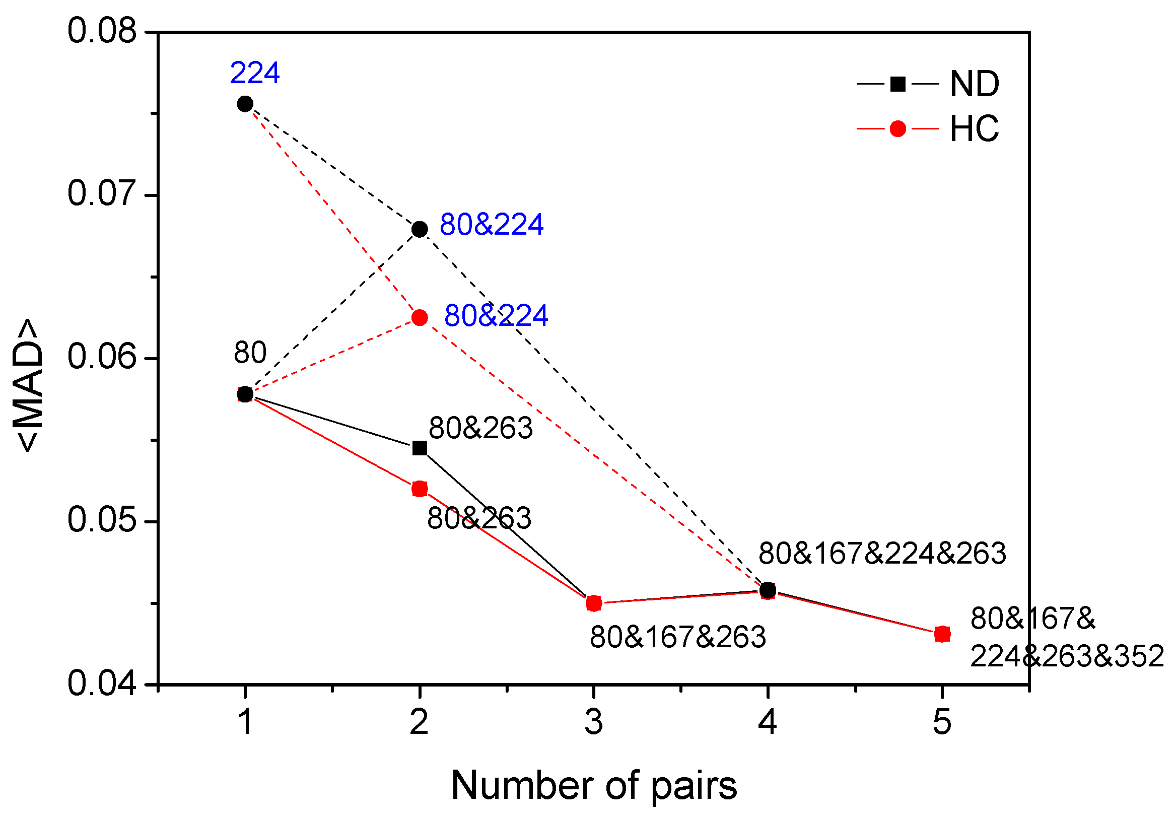
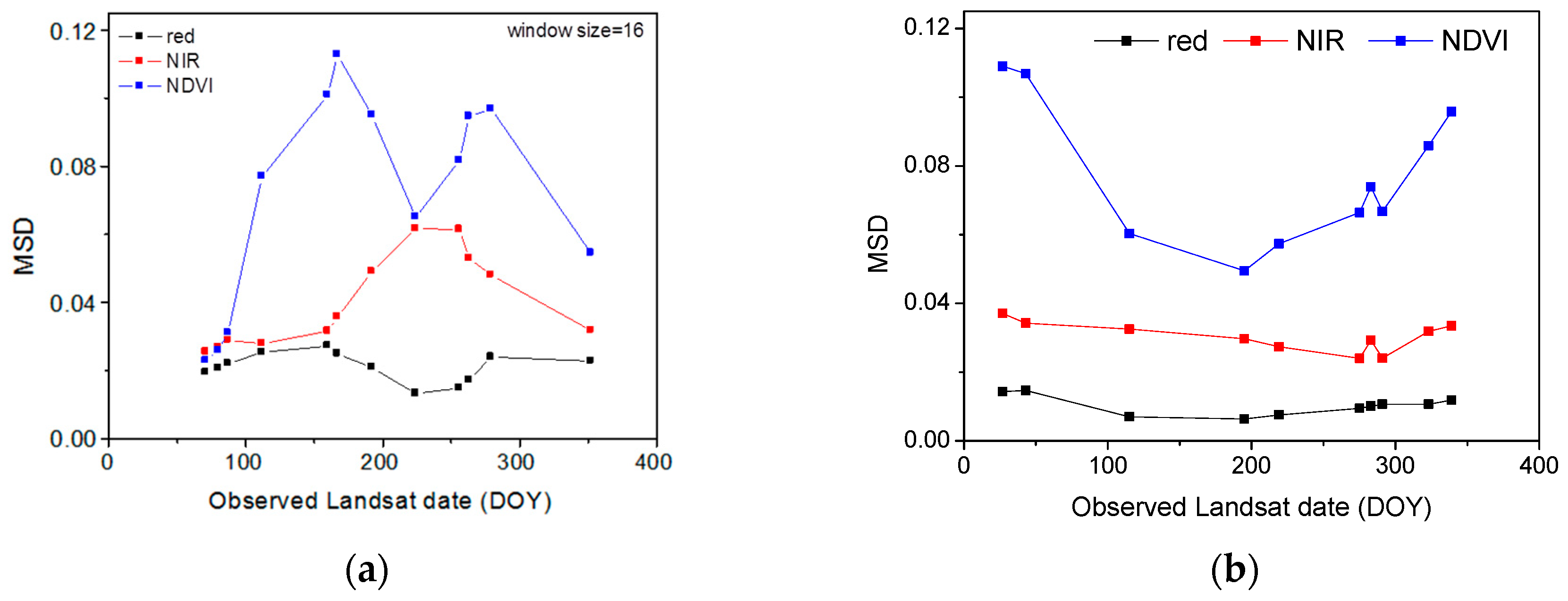
Table 1.
List of the MODIS products used in the study.
| MODIS Products | Spatial Resolution (m) | Temporal Resolution | Description |
|---|---|---|---|
| MOD09GQ | 250 | Daily | Directional reflectance product acquired by Terra (red and NIR bands only) |
| MOD09GA | 500 | Daily | Directional reflectance product acquired by Terra (for all land bands) |
| MYD09GQ | 250 | Daily | Directional reflectance product acquired by Aqua (red and NIR bands only) |
| MYD09GA | 500 | Daily | Directional reflectance product acquired by Aqua (for all land bands) |
| MCD43A1 | 500 | 16-day | Terra and Aqua combined BRDF/Albedo Model Parameters product |
| MCD43A4 | 500 | Daily | Terra and Aqua combined NBAR product |
| MCD43A2 | 500 | Daily | Quality information product for the corresponding MCD43A4 product |
| MCD12Q1 | 500 | Annual | Land cover |
Table 2.
List of MODIS NBAR data products used in the study.
| Product Name | Data Source | Resolution | Coverage | Solar Zenith Angle |
|---|---|---|---|---|
| Terra NBAR | In-house BRDF correction using MCD43A1, MOD09GQ, MOD09GA, MCD12Q1 | 250 m for red and NIR bands | Clear pixels from Terra overpass time | At Terra overpass time |
| Aqua NBAR | In-house BRDF correction using MCD43A1, MYD09GQ, MYD09GA, MCD12Q1 | 250 m for red and NIR bands | Clear pixels from Aqua overpass time | At Aqua overpass time |
| Terra/Aqua combined NBAR | Standard Collection 6 MODIS NBAR products (MCD43A2 and MCD43A1) | 500 m for all Land bands | Clear pixels from 16-day period (at least two clear observations during the period) | Mean solar zenith angle during 16-day period |
Table 3.
Mean view zenith angle (VZA) from MODIS sensors in the study areas on Landsat 7 and 8 overpass dates.
Table 3.
Mean view zenith angle (VZA) from MODIS sensors in the study areas on Landsat 7 and 8 overpass dates.
| Study Areas | Path/Row | Terra + L8 | Terra + L7 | Aqua + L8 | Aqua + L7 |
|---|---|---|---|---|---|
| Site 1 | 028031 | 57.77 | 7.25 | 27.62 | 44.64 |
| 029031 | 60.05 | 4.06 | 38.30 | 40.11 | |
| Site 2 | 025036 | 63.66 | 0.66 | 12.39 | 59.15 |
© 2018 by the authors. Licensee MDPI, Basel, Switzerland. This article is an open access article distributed under the terms and conditions of the Creative Commons Attribution (CC BY) license (http://creativecommons.org/licenses/by/4.0/).
Share and Cite
MDPI and ACS Style
Xie, D.; Gao, F.; Sun, L.; Anderson, M. Improving Spatial-Temporal Data Fusion by Choosing Optimal Input Image Pairs. Remote Sens. 2018, 10, 1142. https://0-doi-org.brum.beds.ac.uk/10.3390/rs10071142
AMA Style
Xie D, Gao F, Sun L, Anderson M. Improving Spatial-Temporal Data Fusion by Choosing Optimal Input Image Pairs. Remote Sensing. 2018; 10(7):1142. https://0-doi-org.brum.beds.ac.uk/10.3390/rs10071142
Chicago/Turabian StyleXie, Donghui, Feng Gao, Liang Sun, and Martha Anderson. 2018. "Improving Spatial-Temporal Data Fusion by Choosing Optimal Input Image Pairs" Remote Sensing 10, no. 7: 1142. https://0-doi-org.brum.beds.ac.uk/10.3390/rs10071142
Note that from the first issue of 2016, this journal uses article numbers instead of page numbers. See further details here.