Radiation Component Calculation and Energy Budget Analysis for the Korean Peninsula Region


1
Research Institute for Radiation-Satellite, Gangneung-Wonju National University (GWNU), Gangneung, 7, Jukheon-gil, Gangneung, Gangwon 25457, Korea
2
Department of Atmospheric and Environmental Sciences, Gangneung-Wonju National University (GWNU), 7, Jukheon-gil, Gangneung, Gangwon 25457, Korea
*
Author to whom correspondence should be addressed.
Remote Sens. 2018, 10(7), 1147; https://0-doi-org.brum.beds.ac.uk/10.3390/rs10071147
Submission received: 31 May 2018
/
Revised: 10 July 2018
/
Accepted: 19 July 2018
/
Published: 20 July 2018
(This article belongs to the Special Issue Earth Radiation Budget)
Abstract
:In this study, a radiation component calculation algorithm was developed using channel data from the Himawari-8 Advanced Himawari Imager (AHI) and meteorological data from the Unified Model (UM) Local Data Assimilation and Prediction System (LDAPS). In addition, the energy budget of the Korean Peninsula region in 2016 was calculated and its regional differences were analyzed. Radiation components derived using the algorithm were calibrated using the broadband radiation component data from the Clouds and the Earth’s Radiant Energy System (CERES) to improve their accuracy. The calculated radiation components and the CERES data showed an annual mean percent bias of less than 3.5% and a high correlation coefficient of over 0.98. The energy budget of the Korean Peninsula region was −2.4 Wm−2 at the top of the atmosphere (), −14.5 Wm−2 at the surface (), and 12.1 Wm−2 in the atmosphere (), with regional energy budget differences. The Seoul region had a high surface temperature (289.5 K) and a of −33.4 Wm−2 (surface emission), whereas the Sokcho region had a low surface temperature (284.7 K) and a of 5.0 Wm−2 (surface absorption), for a difference of 38.5 Wm−2. In short, regions with relatively high surface temperatures tended to show energy emission, and regions with relatively low surface temperatures tended to show energy absorption. Such regional energy imbalances can cause weather and climate changes and bring about meteorological disasters, and thus research on detecting energy budget changes must be continued.
1. Introduction
Global warming refers to the increase in mean global temperatures caused by the increase in greenhouse gasses, which started since the dawn of industrialization at the end of the 19th century. Over the past 100 years, mean global temperatures have increased by approximately 0.6 K, and global warming is accelerating [1,2,3] because of increased positive radiative forcing [4] caused by increases in greenhouse gases in human-centered ecosystems [5] and land changes caused by urbanization [6]. This increase in global mean temperatures causes changes in the energy budget and leads to global energy imbalances. Such a rise in the mean global temperature causes more energy to be emitted from the surface, especially in low altitudes. Subsequently, energy (surplus) that is neither absorbed into the atmosphere nor emitted into space, moves to high latitudes where energy is relatively lower [7]. This process will result in the weather and climate changes. In short, climate change caused by global warming causes changes in ecosystems from polar regions to tropical regions [8,9] and induces natural disasters that threaten human lives [10] as well as the society and economy [11,12]. As such, continuous research and policies are required to monitor and respond to climate change [13,14,15,16,17].
The Earth’s energy balance is the most important factor determining changes in climate and weather, and it is determined by radiation and distribution of radiation [18]. Changes in the global energy budget from the past until the present can be studied using the results of space-based observations, and currently, the global energy budget can be analyzed in detail [19]. In early 1959, the energy absorbed by white and black objects attached to the Explorer-7 satellite was converted into heat and a thermal equilibrium equation was used to calculate global radiation, thus enabling global energy budget observations. Later in the 1970s, the global radiation balance was measured by the Nimbus-7 satellite, and these data became an important component of climate change research, and they were used in analyzing the results of climate models, which were in the initial development phase at that time. Since the 1980s, Earth Radiation Budget (ERB) sensors have been developed to perform more detailed research on the radiation budget, and measurements of both solar radiation reflected by the Earth and emitted longwave radiation have been made possible. Later, sensors known as the Earth Radiation Budget Experiment (ERBE) were installed on the National Oceanic and Atmospheric Administration 9 (NOAA-9) and 10 satellites to perform continued research on the ERB [7]. After the development of ERB, high-resolution satellite sensors, such as ERBE, Scanner Radiometer for Radiation Budget (ScaRaB) [20], and the Clouds and the Earth’s Radiant Energy System (CERES) [21,22,23], were developed. CERES provides radiative fluxes calculated with highly accurate cloud detection [24], and is currently used in energy budget research and various other research. CERES data can be used to improve not only global but also regional climate predictions, and thus, continued data monitoring and accumulation are required [6,25]. With an error rate of less than 2% over 10 years [26], the accuracy of CERES data is higher than that of other radiation data [19,27,28,29]. From the past until the present, numerous studies have used satellite data to extensively research the global energy budget and uncertainty in radiation components [18,19,25,30,31,32,33]. Climate change caused by changes and imbalances in the energy budget are a very important issue not only globally but also regionally. However, analyses on this issue are limited and contain systematic errors because most data on the regional energy budget analysis are not detailed and have a resolution of tens or hundreds of kilometers [34].
This study applied high resolution data to calculate the energy budget of the Korean Peninsula region and demonstrates changes in the regional energy budget and regional energy imbalances. For this purpose, spectral data from the Himawari-8 Advanced Himawari Imager (AHI) [35], as well as meteorological data, sensible heat flux (SHF), and latent heat flux (LHF) from the Local Data Assimilation and Prediction System (LDAPS) analysis field were used. In addition, an algorithm was developed to calculate shortwave radiation components. The algorithm uses the Himawari-8 AHI’s shortwave and longwave spectrals to calculate the reflected shortwave radiation (RSR) and outgoing longwave radiation (OLR), which are radiation components at the top of the atmosphere, and the LDAPS’ meteorological data to calculate downward shortwave radiation (DSR), absorbed shortwave radiation (ASR), downward longwave radiation (DLR), and upward longwave radiation (ULR), which are radiation components at the surface. To improve their accuracy, the radiation components calculated by the developed algorithm were calibrated with the broadband radiation components of the CERES sensor installed on a polar orbit satellite. Based on these results, this study produced an energy budget for the Korean Peninsula region and analyzed changes and regional differences in the energy budget. Section 2 describes the research data in this study. Section 3 describes the radiation component calculations and calibration with CERES data. Section 4 shows the verification of calculated radiation components and the results of the energy budget analysis. Finally, Section 5 presents a summary and conclusions.
2. Data
The radiation components required for calculating the energy budget are as follows: ISR (incoming solar radiation from outside the atmosphere measured at the top of the atmosphere), RSR (radiation reflected into space from the surface, atmosphere, and clouds), DSR (radiation which goes through the atmosphere and reaching the Earth’s surface), ASR (the net radiation, excluding radiation reflected to the atmosphere and space by albedo at the surface), ULR (radiation absorbed by the surface and emitted back to the atmosphere and space), DLR (radiation absorbed by the atmosphere and clouds and emitted back towards the surface), OLR (radiation emitted from the surface, atmosphere, and clouds toward space), and SHF and LHF (non-radiative fluxes). This study used satellite data and the analysis field of a numerical weather prediction (NWP) model to calculate the energy budget.
AHI channel data from the Himawari-8 geostationary satellite [35] were used to calculate RSR (AHI 1–6 channels) and OLR (AHI 8 and 15 channels). Himawari-8 was launched in 2014 and floats over the equator at 140.7°E and 0°N, observing a hemisphere area, which includes the Korean Peninsula region. The AHI sensor has very similar channel characteristics as the Advanced Meteorological Imager (AMI) of South Korea’s next-generation satellite, the Geostationary Korea Multi-Purpose satellite 2A (GK-2A, scheduled to launch in 2018) [36]. It has 6 shortwave channels and 10 longwave channels and provides data of 2 km × 2 km resolution at 10-min intervals [37]. This sensor provides radiance observed through a narrow band; therefore, the broadband radiation component was calculated through an empirical method (refer to Section 3).
The radiation components on the surface were calculated by an empirical method using LDAPS data of the Unified Model (UM) [38]. This model was introduced by the United Kingdom Meteorological Office (UKMO) and is currently being used by the Korea Meteorological Administration (KMA). The model provides data on 86 variables regarding isobaric surface and surface for each 1.5 km × 1.5 km grid cell at 3-h intervals, which are sufficient for the purpose of the study. Similar numerical weather prediction models, such as the National Centers for Environmental Prediction (NCEP) Final (FNL) (https://rda.ucaredu/datasets/ds083.2) and ERA-Interim [39], provide the required meteorological data but their spatiotemporal resolution is not sufficient (6-h intervals, 1° × 1°). Therefore, they were not used as input data.
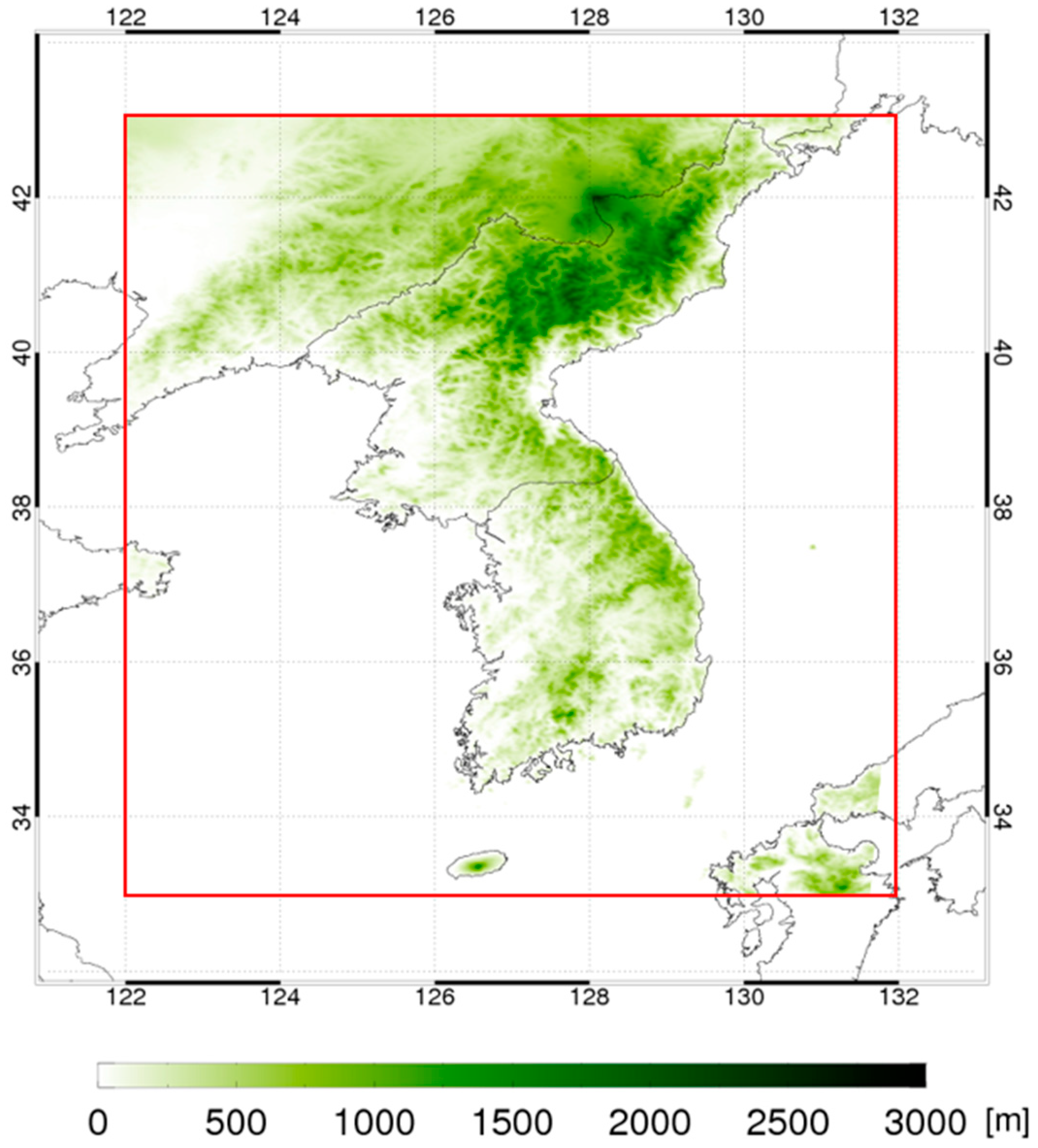
In this study, changes in the energy budget of the Korean Peninsula region (122–132°E, 33–43°N; Figure 1) from 1 January 1 to 31 December 2016 were analyzed. This period was selected for the purpose of collecting latest data (Himawari-8 AHI data collection was possible from August 2015) required for energy budget calculations. In addition, the temperature of the Korean Peninsula region in that year was 286.6 K, approximately 1 K higher than the mean temperature from 1981 to 2010 (30 years); however, the precipitation (1272.5 mm), number of days with precipitation (109 days), and cloud cover (53%) were similar to normal year mean [40,41]. Hence, it was thought that the data selected would show the typical energy budget of the Korean Peninsula region. For the radiation component calculations, data were produced eight times per day at 3-h intervals starting at 0000 UTC based on the temporal resolution of LDAPS data. Some Himawari-8 AHI data are missing for this time, and if shortwave radiation or longwave radiation component data were missing two times or four times, respectively, out of eight times, the day was excluded from the analysis period. As such, January 14, 17, 20, 21, and 24; February 9, 10, and 27; April 10, 17, 18, and 19; May 11; June 21; September 18; and December 24 were excluded from the analysis (for a total of 350 days). In addition, the spatial grid was created based on Himawari-8 AHI’s 2 km × 2 km grid.
CERES is a next-generation ERB sensor, and it is the only sensor on currently operating satellites that provides shortwave (0.2–5 μm) and longwave (5–100 μm) broadband radiation [26]. Therefore, the radiation components calculated by the algorithm developed in this study were compared to broadband radiation data from CERES. CERES is installed on the Terra, Aqua, and Suomi National Polar-Orbiting Partnership (NPP) platforms. The data used for verification and calibration of the calculated radiation components were obtained from the Terra CERES single scanner footprint (SSF) Level2 Edition3A (Ed3A) [42], which observes the Korean Peninsula region in 16-day cycles. Terra CERES data were used because it passes the Korean Peninsula around 1200 local standard time (LST) when the maximum radiation occurs (nighttime verification data for longwave radiation were collected at around 0000 LST). In the verification and calibration, the spatial resolution of the calculated data was set at 20 km × 20 km to match that of CERES data. The radiation components were calculated at 3-h intervals and interpolated to match the CERES observation times. For the calibrated radiation components, an analysis was performed on the CERES SYN1d Ed3A, which provides daily mean data at a spatial resolution of 1° × 1°, and the daily mean time series data, and then the calculation accuracy was evaluated.
CERES Energy Balanced and Filled (EBAF) Ed4.0 [43,44] and Modern Era Retrospective Analysis for Research and Applications Version 2 (MERRA-2) M2T1NXFLX data [45] were used for comparing energy budgets. SHF and LHF data from MERRA-2 were used because CERES data do not provide them. MERRA-2 data include atmosphere reanalysis data from the 1980s and after, and they are used in conjunction with GEOS-5 data [46]. These data have several advantages for analysis in that their accuracy has been confirmed by [47] and [48] and their grid size is smaller than that of other global models [49]. The spatial resolutions of CERES EBAF and MERRA-2 data are 1° × 1° and 0.625° × 0.5°, respectively. Therefore, the spatial resolutions were modified to match that of CERES for the analysis.
3. Calculation of Radiation Components and Energy Budget
Section 3.1 and Section 3.2 describe the algorithm for calculating the shortwave/longwave radiation components needed to calculate the energy budget. In Section 3.3, the calculated radiation components are compared and calibrated. Section 3.4 describes the methods for calculating the energy budget at the top of the atmosphere, the surface, and the atmosphere.
3.1. Shortwave Radiation Compoents
3.1.1. ISR
To calculate the net radiation at the top of the atmosphere, ISR was calculated using the method developed by [50], as shown in Equations (1)–(3).
Here, is the day angle, is the Julian day, is the eccentricity, is the solar zenith angle (SZA), and is the solar constant, which is 1361 Wm−2 [51].
3.1.2. RSR
RSR is ISR that enters from the top of the atmosphere and is reflected back out of the atmosphere by the surface, the atmosphere, and clouds. It was calculated using Himawari-8 AHI’s shortwave channels (channels 1–6). The broadband albedo at the top of the atmosphere was calculated, and the RSR was calculated according to the sun zenith angle and eccentricity as in Equations (4) and (5). Here, the required regression coefficients were calculated via the linear relationship between the narrowband reflectance and the broadband reflectance for each channel [52]. In addition, because the atmosphere is anisotropic, a chart of coefficients for each direction was created, taking into account the sun zenith angle, viewing zenith angle, and relative azimuth between the sun and the satellite [53,54]. For the relationship between the narrowband reflectance and the broadband reflectance, the Santa Barbara DISORT Atmospheric Radiative Transfer (SBDART) [55] was used to simulate various atmosphere conditions that may be present in the actual atmosphere (Table 1), and the calculated results were used [56].
Here, is the broadband albedo at the top of the atmosphere; is the viewing zenith angle (VZA); is the relative azimuth angle (RAA); – are the regression coefficients according to the SZA, VZA, and RAA required for calculating ; is the narrowband reflectance; and the subscripts are the central wavelengths for each of Himawari-8 AHI’s shortwave channels.
3.1.3. DSR and ASR
DSR is the shortwave radiation which through the Earth’s atmosphere and arriving at the surface, excluding RSR, which is reflected at the top of the atmosphere. ASR is the net shortwave radiation excluding the radiation reflected to the atmosphere or outside the atmosphere due to surface albedo () [57]. ASR is defined as , but surface albedo is one of the meteorological data variables with high uncertainty. Consequently, its values widely vary depending on the time and location, and it is difficult to use highly accurate data at each moment because of limitations in the provided data [58]. Therefore, in this study, surface albedo data were not used, and the linear relationship between RSR and total precipitable water (TPW) was used to calculate DSR (Equations (6)–(8)) and ASR (Equations (9)–(11)) [59,60]. Here, the radiative transfer model was simulated and the relationships between radiation and meteorological variable were determined, as shown in Table 2. The created regression coefficients (– and –) are shown in Table 3.
3.2. Longwave Radiation Components
3.2.1. OLR
OLR is longwave radiation at the top of the atmosphere emitted by the Earth’s surface, the atmosphere, and clouds. It was calculated using Himawari-8 AHI’s longwave channels (channels 8 and 15). Based on the high correlation between narrowband irradiance and broadband irradiance, similar to that in RSR [61], narrowband radiance was converted to narrowband irradiance considering the atmosphere’s anisotropy via Equations (12)–(15) [62,63], and the converted narrowband irradiance was converted into broadband irradiance [64]. The radiative transfer model was simulated using parameters as shown in Table 4, and the coefficients developed by [65] were used in the equations (Table 5 and Table 6).
Here, is the irradiance (the subscripts are the central wavelengths of Himawari-8 AHI’s channels 8 and 15); is the radiance; – are the regression coefficients for converting radiance to irradiance; and – are the regression coefficients for calculating OLR.
3.2.2. DLR
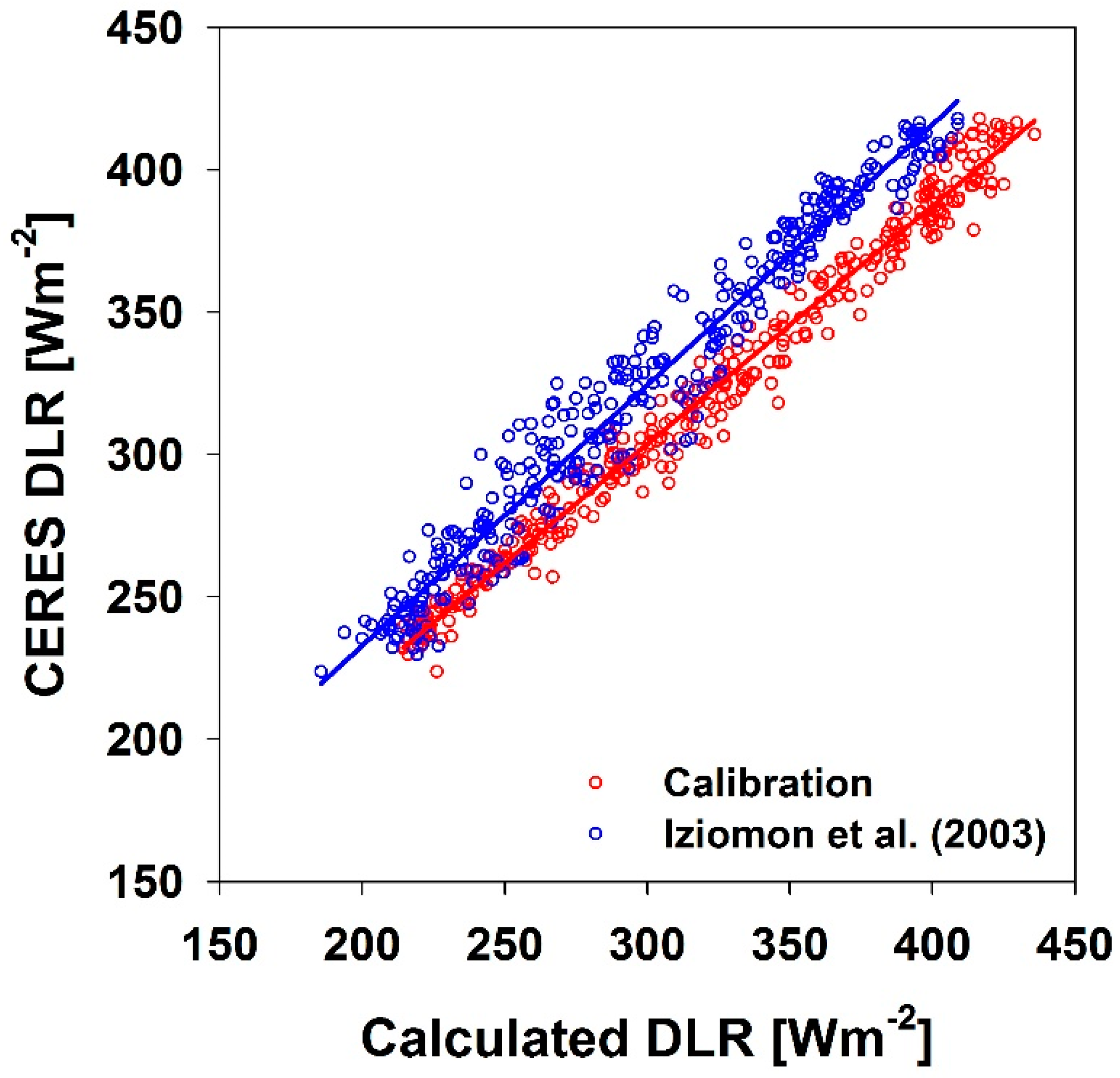
DLR is longwave radiation emitted from clouds and the atmosphere that arrives at the surface. It can be calculated using its high correlation with weather variables such as the temperature near the surface and cloud information, such as total cloud cover, cloud emissivity, and cloud base temperature [66,67,68,69,70]. This study used the method presented by [71], in which DLR is calculated empirically using air temperature, total cloud cover, and water vapor pressure (Equation (16)). However, directly using their method resulted in discontinuous DLR calculations at lowland and mountain sites and underestimations of DLR due to total cloud cover. Therefore, the method was modified using the relationship between air temperature and total cloud cover to calibrate the coefficients, as in Equation (17). Different results were obtained using the modified method, as shown in Figure 2. Here, the data used in this study (total 350 days) were compared with CERES DLR. Using the method of [71], the obtained Bias, RMSE, and R were −24.54 Wm−2, 27.34 Wm−2, and 0.98, respectively. The results were improved to −0.14 Wm−2, 12.93 Wm−2, and 0.99 using the modified method.
Here, the , , and coefficients are respectively 0.35, 10.0 K hPa−1, and 0.0035 in lowland areas with an altitude of less than 212 m, and they are 0.43, 11.5 K hPa−1, and 0.0050 in mountainous areas. is the air temperature; is the water vapor pressure; is the cloud cover; and – are the coefficients for calculating DLR. – are the coefficients from when the smallest difference exists between the CERES DLR and the results of calculating Equation (17) using MERRA-2 air temperature and water vapor pressure and CERES total cloud cover, as shown in Table 7.
3.2.3. ULR
ULR is DLR reflected from the surface and longwave radiation emitted from the surface. It can be calculated using Equation (18).
Here, is the surface emissivity; is the surface temperature; and is the Stefan–Boltzmann constant (5.67 × 10⁻⁸ Wm−2 K−4). The surface emissivity for calculating ULR is distributed within the range of 0.9 and 1, depending on the properties of the surface. It is a core component in calculating ULR [72], but it involves high uncertainty depending on the surface properties and time and location. Furthermore, if it is assumed to be a constant (long-term mean), a maximum difference of over 10% with the observed surface emissivity may result [73,74]. Therefore, in this study, an algorithm to calculate ULR is presented without using surface emissivity which has a relatively higher uncertainty than other meteorological data, as with ASR.
Infrared atmospheric transmittance () is defined as a ratio of ULR and OLR (Equation (19)), and ULR can be expressed as Equation (20). That is, ULR can be calculated even without surface emissivity data by using OLR and infrared atmospheric transmittance.
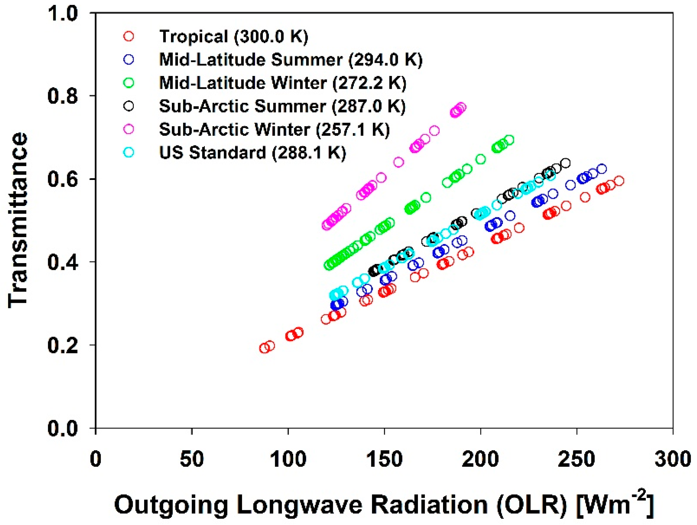
When the results of the simulation for calculating OLR from Section 3.2.1 were used, atmospheric transmittance showed a linear relationship with OLR as shown in Figure 3, and the slope showed other features according to surface temperature. Ultimately, the relationship between the three variables can be described by Equation (21). In this study, only OLR and surface temperature were used to calculate ULR.
Here, − are the regression coefficients for calculating the ULR, as shown in Table 8.
3.3. Calibration Using CERES and MERRA-2 Data
The radiation components calculated in this study were compared to the radiation of Terra CERES SSF Level2 Ed3A. Terra CERES observes the Korean Peninsula region at approximately 16-day intervals. The example shown in Table 9 was set up to perform the analysis. Shortwave radiation components were observed only during the daytime, and thus only data from 0230 UTC were used. Longwave radiation components were observed during both daytime and nighttime, and thus data from 0230 UTC and 1330 UTC were used. Here, cases with missing Himawari-8 AHI data were excluded from the analysis.
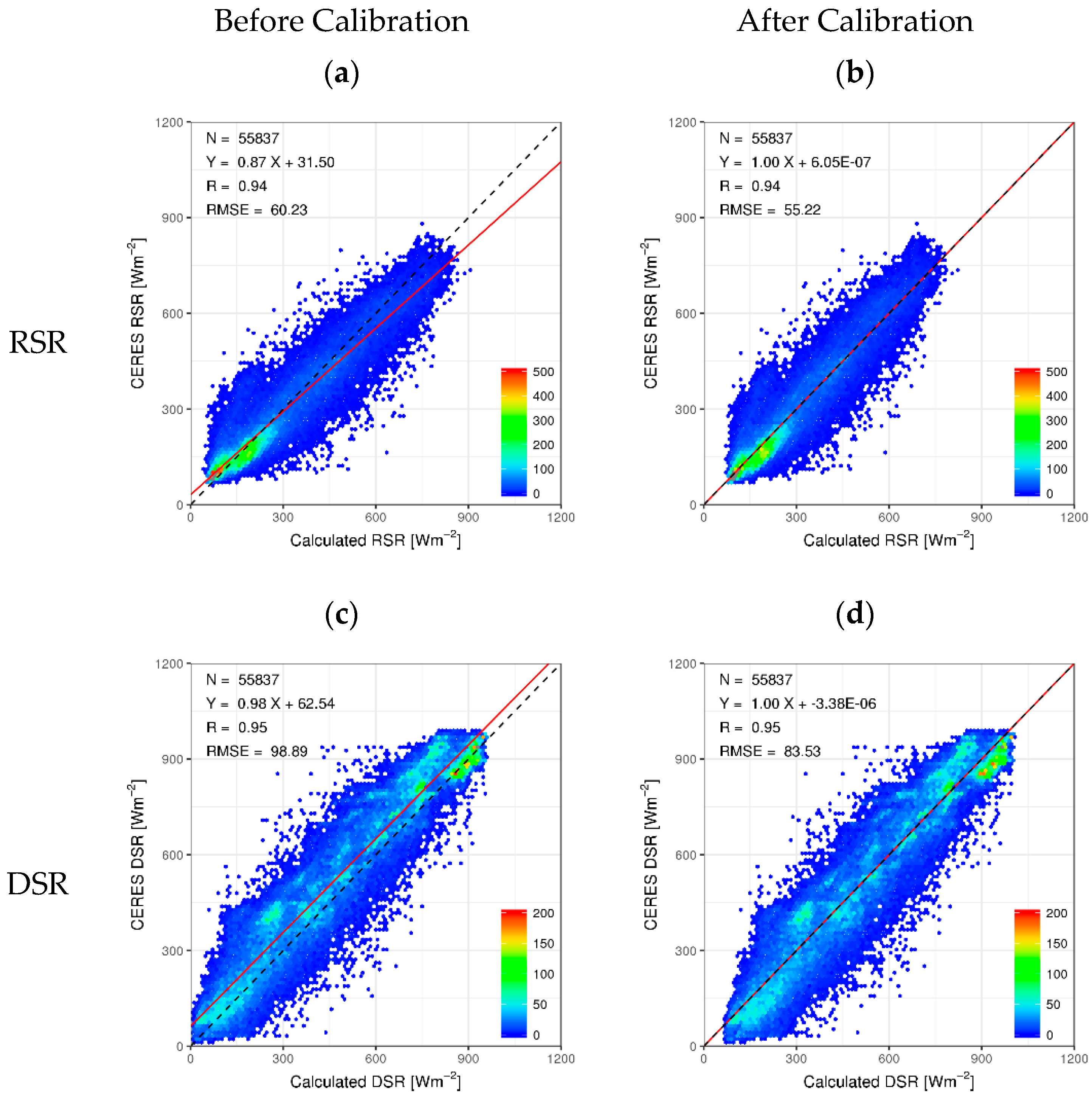
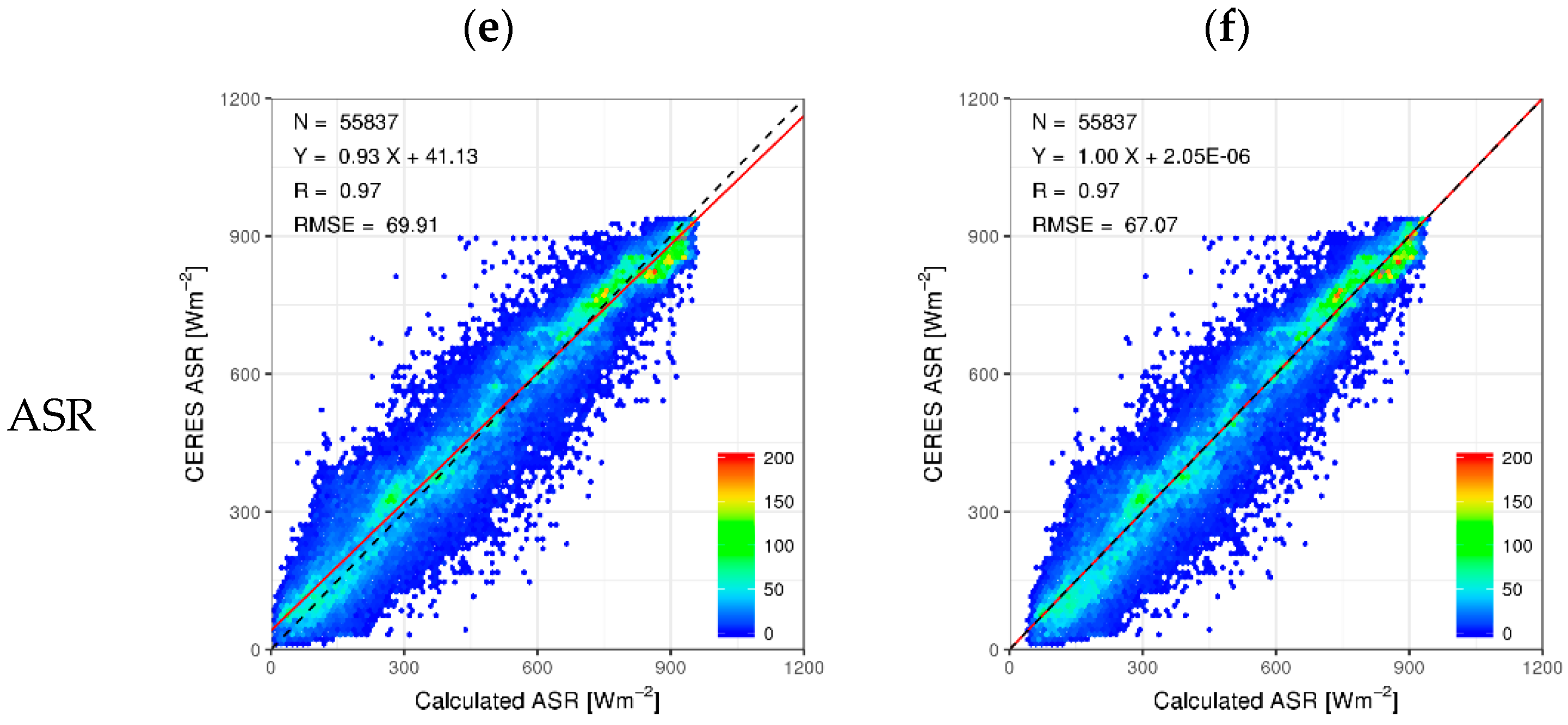
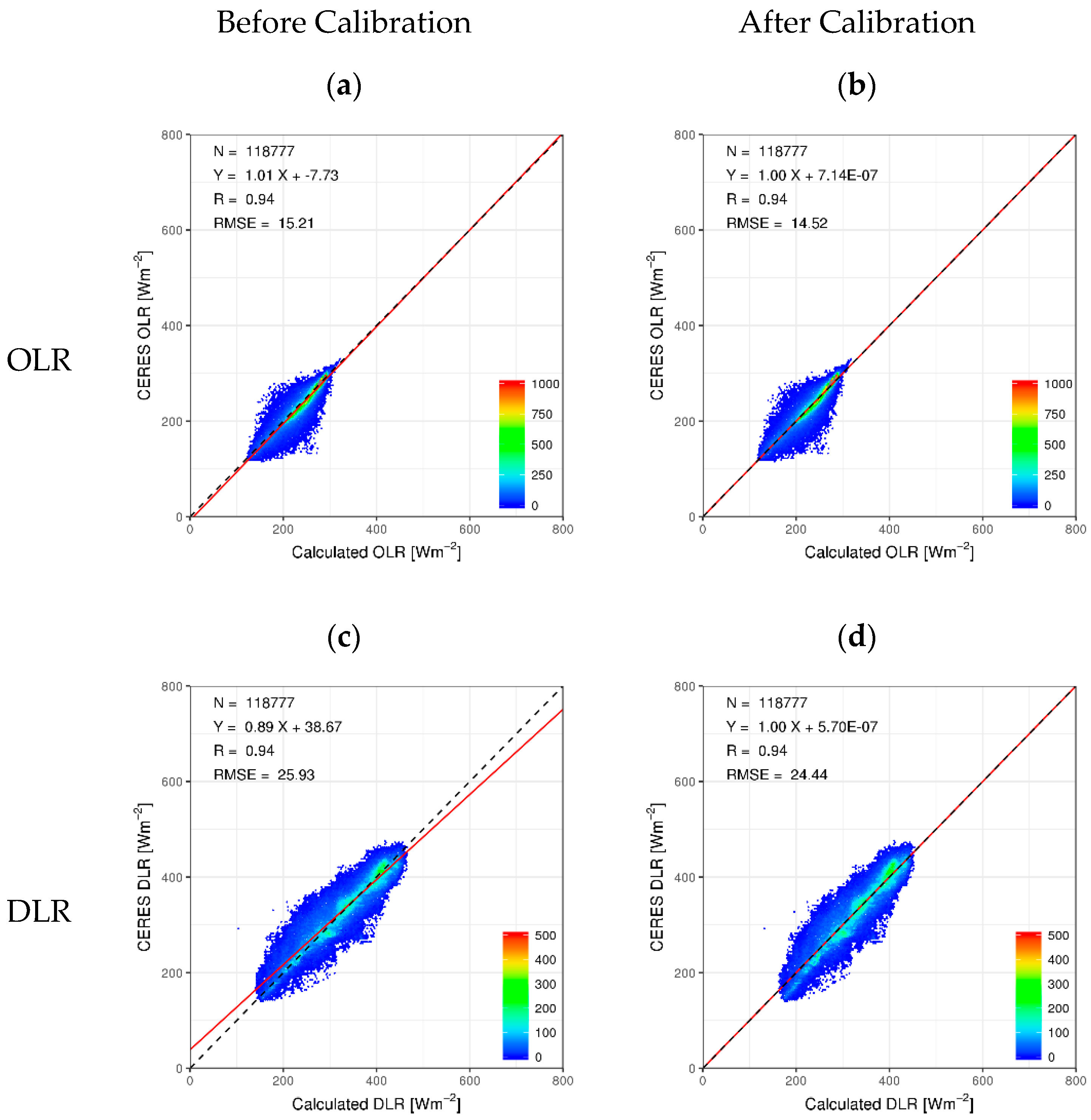
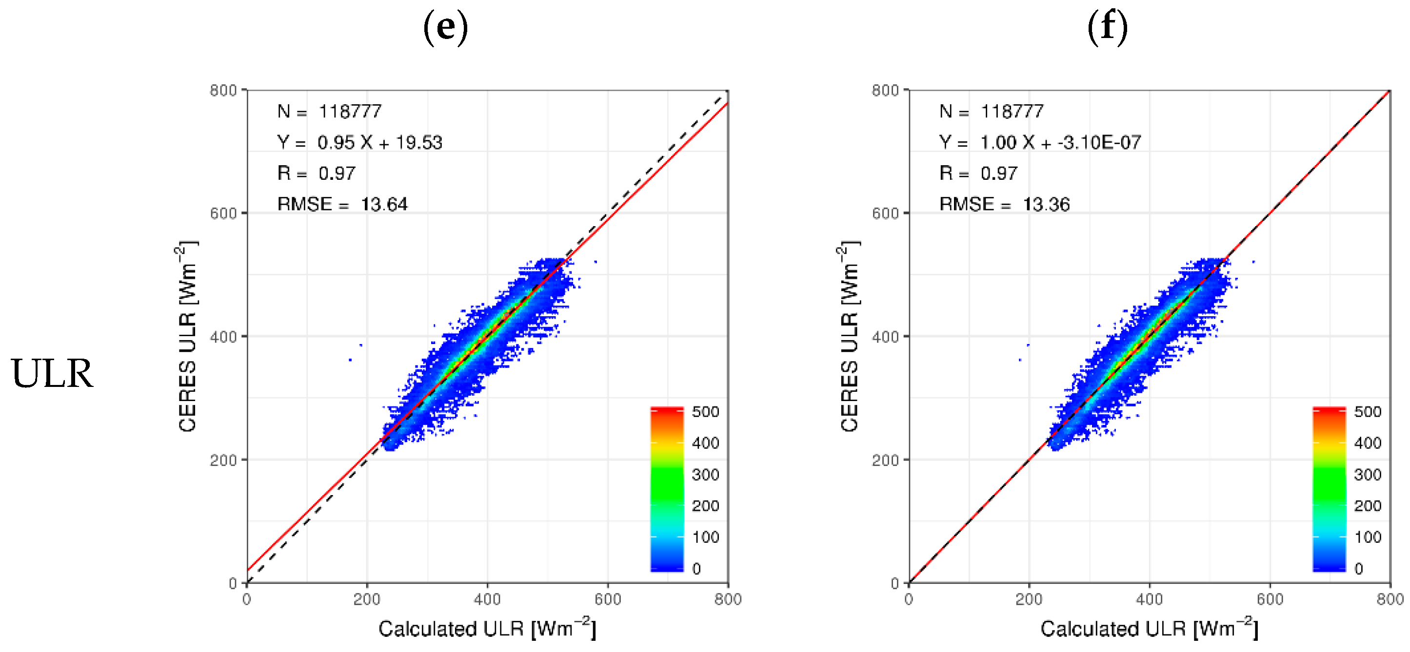
For the calculated radiation components, data were generated at 3-h intervals starting at 0000 UTC. Therefore, data from 0000 UTC and 0300 UTC or 1200 UTC and 1500 UTC were interpolated to match the times of the verification data, and the analysis was performed. Furthermore, the calculated radiation components were calibrated using a linear relationship (). The calibration was performed using highly accurate data from long-term observations to compensate for nonlinearity and various unconsidered problems that may arise in the empirical method, the calculation accuracy could be improved [75,76]. The before and after calibration results for each radiation component showed that the difference between the after calibration results and the CERES data was smaller than the difference between the before calibration results and the CERES data, as shown in Figure 4 and Figure 5. In the case of shortwave radiation, the radiation was large, and there was a large difference in the radiation irrespective of the existence of clouds; thus, the RMSE was larger than that of longwave radiation. That is, interpolation was performed based on the spatiotemporal resolution of CERES, and thus, the RMSE was found to be large. Nevertheless, the calibrated radiation components showed a high concentration along the 1:1 line. The slopes were all calibrated to 1, and the radiation showed a high correlation coefficient with the CERES radiation at over 0.94.
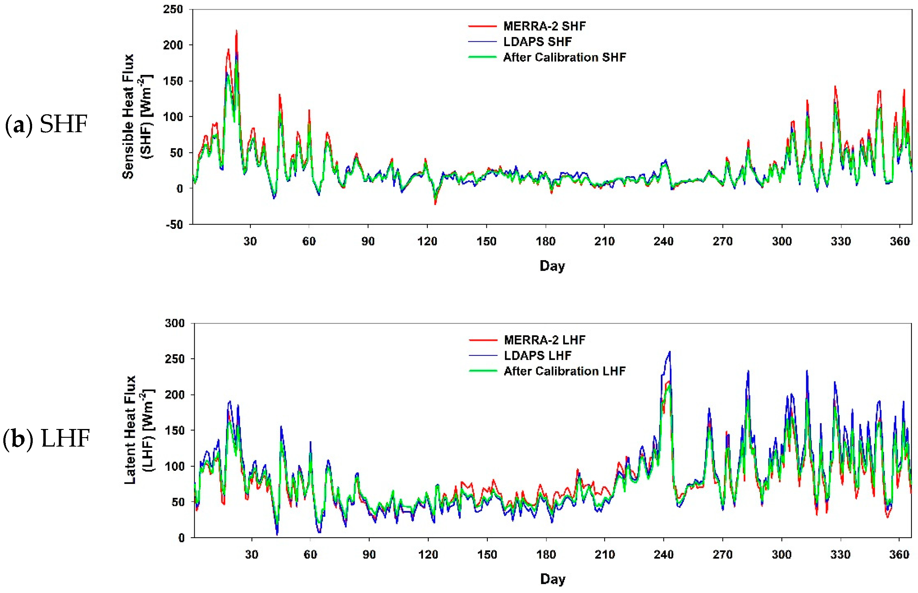
In the calculation of the energy budget at the surface, large fluxes of LDAPS SHF and LHF were found to be emitted during spring and winter due to the effect of the Kuroshio current, as shown in Figure 6. LHF showed a different trend than SHF due to the effects of typhoons, which moved northward near the Korean Peninsula during summer and fall (e.g., Lionrock at the end of August and Namteheun at the beginning of September). For verifying SHF and LHF, values from a real ship and remote sensing can be compared, but observation data is very rare, and remote sensing includes a relatively large flux of calculation errors; therefore, a comparison was normally made with model results [77]. However, when SHF and LHF calculated from model results were compared to the real observed values, SHF included ~25% uncertainty and LHF included 10% uncertainty [25,78]. Therefore, in order to improve the accuracy of the LDAPS SHF and LHF, they were calibrated with MERRA-2, which performs global data assimilation. Before calibration, SHF and LHF had RMSE values of 8.56 Wm−2 and 15.70 Wm−2, respectively, when compared to the MERRA-2 data, and after calibration their RMSE improved to 4.35 Wm−2 and 9.62 Wm−2.
3.4. Energy Budget
The radiation components described in Section 3.1 and Section 3.2 and LDAPS SHF and LHF were used to calculate the energy budget as described below. Equation (22) is the net radiation at the top of the atmosphere (), which can be shown as the difference between the incoming solar radiation () and the reflected shortwave radiation at the top of the atmosphere () and the emitted longwave radiation ().
The net radiation at the surface is defined by the change in thermal energy over time, as shown in Equation (23), and it can be considered as the difference in shortwave net radiation and longwave net radiation () and the difference in SHF and LHF [79,80]. Following the law of conservation of energy, the net radiation at the surface () achieves an energy balance as in Equation (26), and it can be expressed as Equation (27).
Here, is the evaporative latent heat of the water vapor.
The difference between the net radiation at the top of the atmosphere and the net radiation at the surface is expressed as the net radiation in the atmosphere (), as in Equation (28).
4. Results
4.1. Verification of Calculated Radiation Components
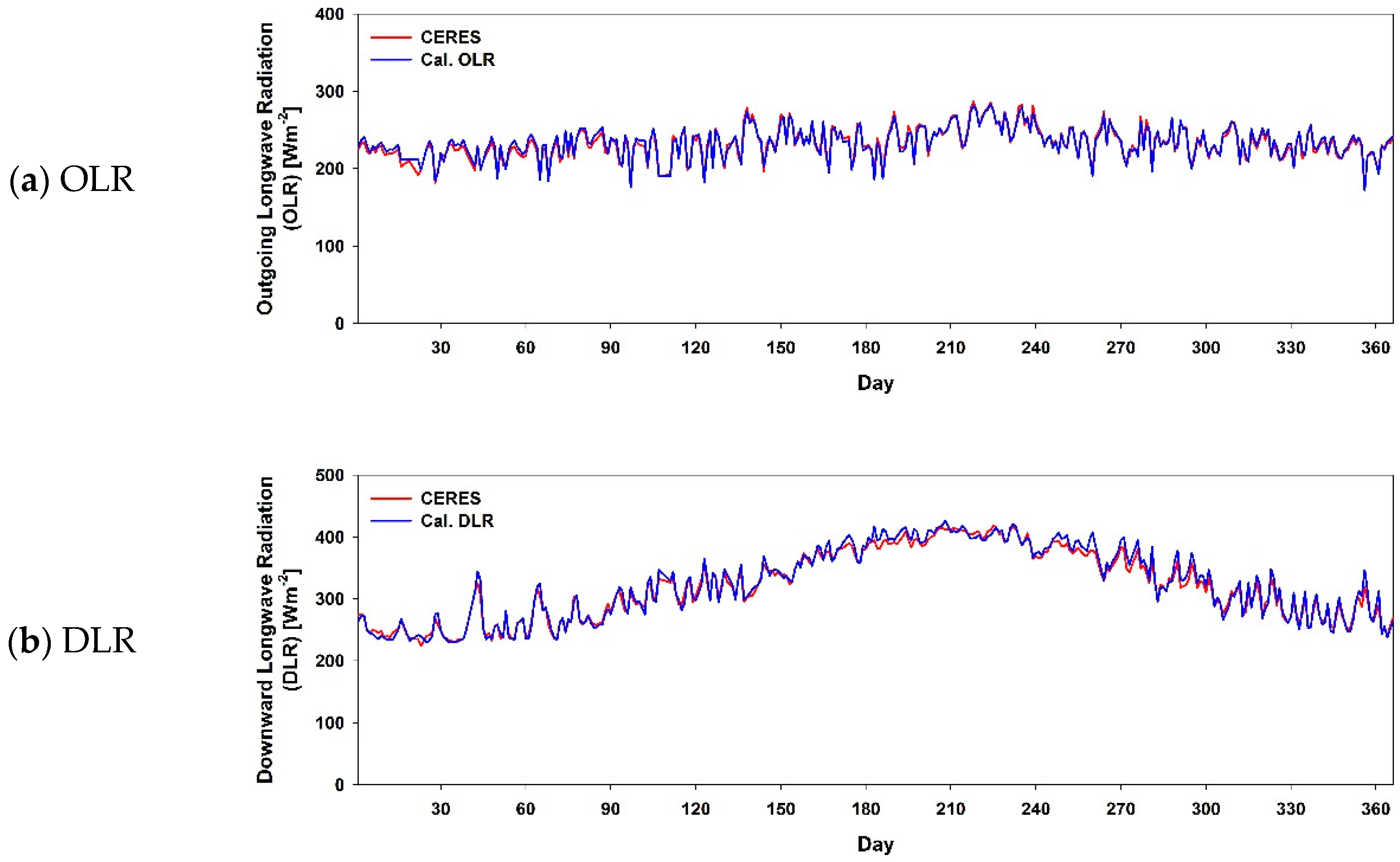
For the calibrated radiation components, a 2016 daily mean time series analysis was performed for the Korean Peninsula region before calculating the energy budget, as shown in Figure 7 and Figure 8. Figure 7 shows the time series distribution of shortwave radiation components, revealing a large amount of ISR and RSR on the Korean Peninsula in the summer season. RSR varied depending on total cloud cover. In August (Julian day 214–244), the total cloud cover was 46%, which was less than the mean total cloud cover in summer and fall, which was 57%. Therefore, RSR was low. In contrast, DSR and ASR showed the opposite trend. There were large longwave radiation components in summer and fall when the surface temperature was high, and the radiation became smaller in spring and winter (Figure 8). OLR showed no significant variations throughout the year, but there were differences in DLR and ULR according to the temperature near the surface. The calculated radiation components showed a similar time series distribution as the CERES radiation components, and the differences between CERES and calculated radiation are shown in Table 10.
ISR was very similar to the radiation observed by the Total Irradiance Monitor (TIM) onboard NASA’s Glory satellite [81], and the radiation component calibrated in this study showed a percent bias () of less than 3.5%. The RSR and OLR showed a bias of approximately 1 Wm−2, but this was calculated based on real observed satellite data, and thus, its calculation precision was higher than that of other radiation components. The radiation components calculated using meteorological data showed variations according to the accuracy of the input data, leading to large differences with CERES data [58,73,82]. In the case of DSR and ASR, the broadband albedo at the top of the atmosphere (), which was used as input data, was 0.31. This value is the same as that of CERES, but the LDAPS TPW (1.69 cm) was 0.26 cm smaller than CERES TPW (1.95 cm). That is, the reduction in radiation due to TPW was underestimated, and thus, DSR and ASR were larger than that of CERES data during summer when TPW is high (Figure 7c,d). The bias and RMSE of DSR with the CERES data were 12.16 Wm−2 and 20.10 Wm−2, respectively, and those of ASR were 12.13 Wm−2 and 18.42 Wm−2, which were larger than in other seasons. In the case of DLR and ULR, there were differences in the calculated radiation according to the temperature near the surface (air/surface). For DLR, there was no difference between the calculated mean air temperature (285.56 K) and the MERRA-2 value (285.26 K). However, for ULR, there was a difference of approximately 1.25 K between the calculated surface temperature (286.97 K) and the CERES value (285.73 K). This difference was largest during winter when the CERES ULR and the calculated ULR had bias and RMSE of 8.72 Wm−2 and 9.04 Wm−2, respectively, which were larger than those during other seasons (Figure 8c). In this study, the calculated radiation values were calibrated to achieve high-accuracy, high-resolution energy budget. However, the calculated radiation values contain uncertainty and inaccuracies due to the differences in the input data described here. Therefore, the input data must be improved through future research.
In addition to satellite data, DSR and DLR data observed from a pyranometer (CMP21) and pyrgeometer (CGR3) at the Gangneung-Wonju National University (GWNU) observatory (128.9°E, 37.8°N) [83] were used to verify for calculated DSR and DLR in this study. CERES data were also compared with GWNU observation data. As a result, both the CERES and the calculated DSR and DLR showed a time series distribution as shown in Figure 9, and it was similar to the distribution of the GWNU observation data, and the statistical analysis results are shown in Table 11. The correlation coefficients with observed data were similar or higher for the calculated results than CERES, and bias and RMSE were approximately 10 Wm−2 less than CERES. Such a difference in the regional radiation is thought to have occurred because the grid size provided in the CERES data is relatively larger, at 1° × 1°. Therefore, the radiation data with 2 km × 2 km grid, which was suggested by this study for a regional analysis, seems to be more appropriate than the CERES data.
4.2. Energy Budget of the Korean Peninsula Region
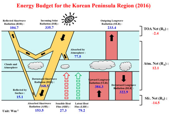
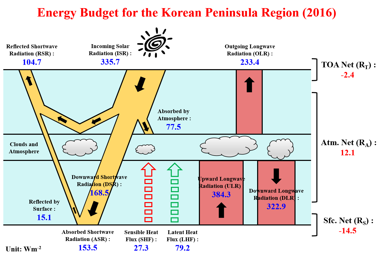
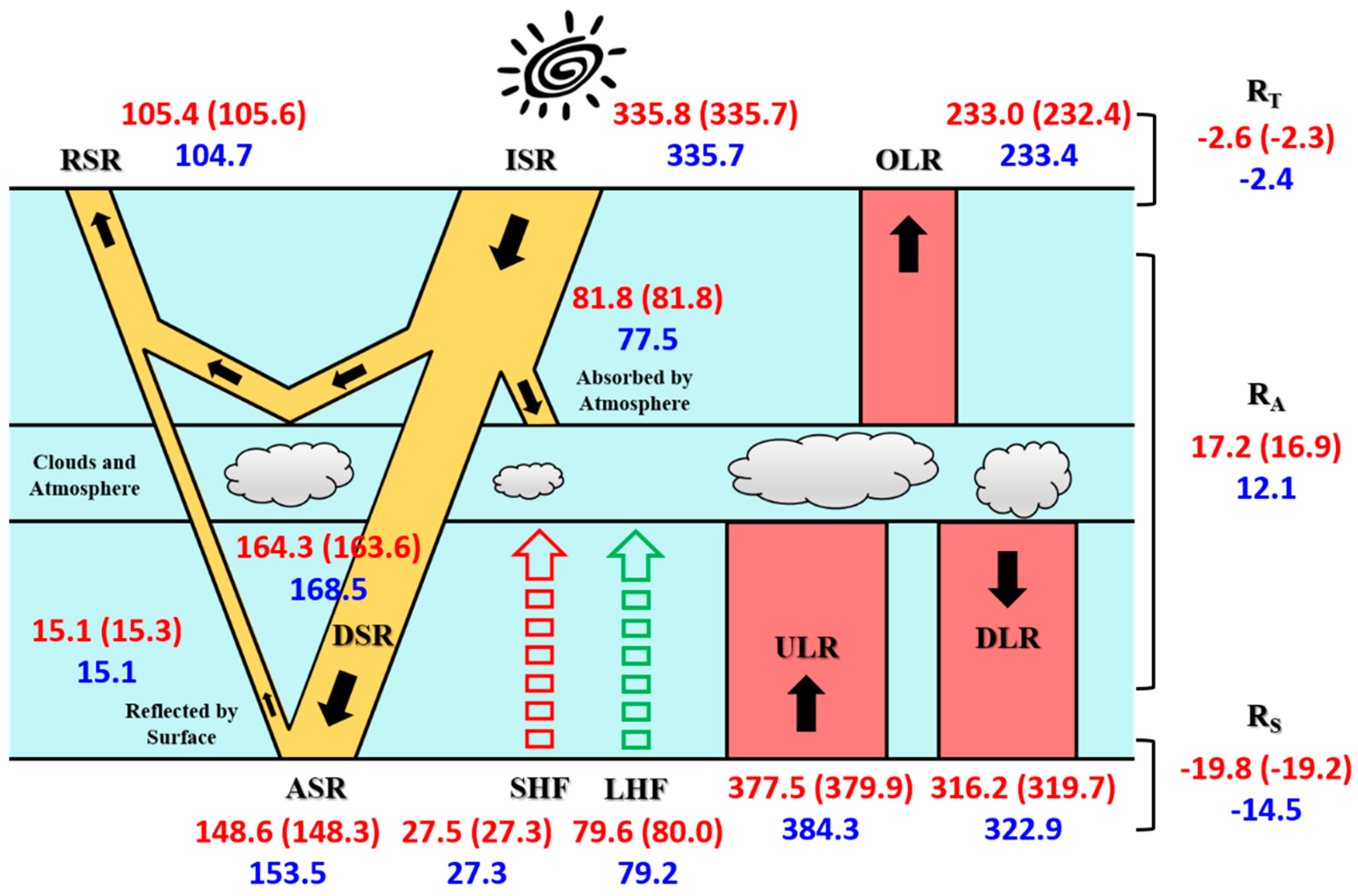
As ISR passes through the Earth’s atmosphere and arrives at the surface, it is absorbed or reflected by clouds, etc., and DSR, which also arrives at the surface, is partially reflected by surface albedo. ASR, which excludes reflected radiation from DSR, is absorbed by the surface and heats the surface. The heated surface emits ULR, and SHF and LHF occur due to variations in the temperature and water vapor near the surface. Furthermore, RSR, which is reflected by the surface, atmosphere, and clouds, and the emitted OLR achieve a balance with the ISR (the energy balance between ISR, RSR, and OLR actually variations periodically [84]). The energy absorbed by the atmosphere in this process is the difference between ISR, RSR, and ASR, and this energy is emitted as DLR or OLR [79,80]. In addition, the difference between DSR and ASR can be shown as Upward Shortwave Radiation (USR). From the results of calculating the radiation components in this study, the energy budget for the Korean Peninsula region could be obtained, as shown in Figure 10. The calculated results showed radiation components and an energy budget similar to CERES and MERRA-2. When the radiation components calculated in this study were compared with long-term mean global radiation components and energy budgets [25,85], RSR was approximately 2.7 Wm−2 larger and ISR and OLR were approximately 5.0 Wm−2 smaller. In polar regions, ISR is very small, approaching 0 Wm−2; therefore, even though the annual mean total cloud cover of the Korean Peninsula region was 47.4%, which is smaller than the global mean of 67.5%, its RSR was larger than the global mean. Conversely, equatorial regions have a large ISR, and the surface and atmosphere temperatures are high; thus, ISR and OLR are large. As a result, ISR and OLR in the Korean Peninsula region were smaller than the global mean. RSR was 2.7 Wm−2 larger and ISR and OLR were approximately 5.0 Wm−2 smaller [86]. Nevertheless, the Korean Peninsula lies in a region where a relative energy balance is achieved at the top of the atmosphere with a of −2.4 Wm−2. Regarding radiation components at the surface, shortwave radiation DSR was 16.5 Wm−2, and ASR was 9.0 Wm−2, whereas longwave DLR was 15.1 Wm−2, and ULR was 13.2 Wm−2. In tropical regions, the absorbed and emitted radiation at the surface is very large, so the Korean Peninsula region’s surface radiation component values were smaller than the global mean. Conversely, SHF+LHF was approximately 5.0 Wm−2 larger than the global mean because the Korean Peninsula region is affected by the Kuroshio current, and it has high sensible heat and latent heat [77,87]. Because of this radiation balance, a negative net radiation (energy emission) occurred, with an of −14.5 Wm−2. This energy is absorbed into the atmosphere or emitted outside of the atmosphere. The energy absorbed in the atmosphere is used during land and sea energy exchange/transport [19,88] or it increases the temperatures of regions that have a relatively low temperature distribution and is transported to polar regions such that the global mean energy budget achieves a balance [7].
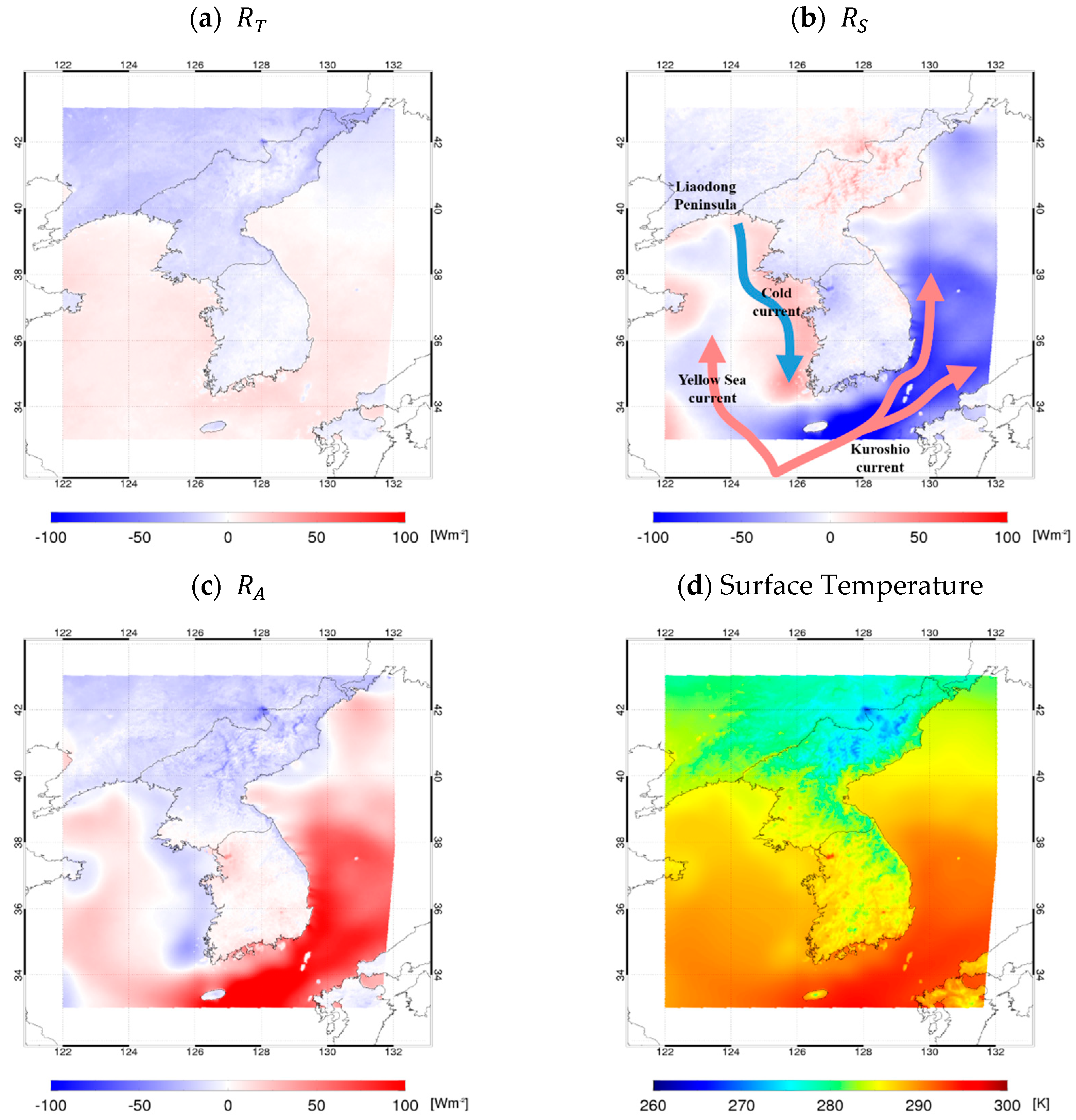
The annual mean , , and of the Korean Peninsula region for 2016 are shown in Figure 11. At lower latitudes, ISR and OLR are larger than RSR and the surface albedo of the land is larger than that of the sea, and thus RSR of the land becomes larger than that of the sea. Regarding , the positive net radiation becomes large in low-latitude seas, and the negative net radiation becomes large in high-latitude land. was similar to the distribution of SHF+LHF, and there was a particularly strong negative net radiation of over 80.0 Wm−2 in the South Sea and East Sea regions, which are affected by the Kuroshio current. In the West Sea region, the Yellow Sea current—which is derived from the Kuroshio current—flows in, but as the ocean current circulates, the cold current flows from the Liaodong Peninsula and moves along the west coast (refer to Figure 11b). Therefore, the seawater temperature is low and a positive net radiation occurs. As such, the in Figure 11c,d showed energy absorption in regions with a large temperature variation in different seasons and higher surface temperature, and conversely it showed energy emission in regions with a small temperature variation and lower surface temperature. That is, was shown positive net radiation in metropolitan regions (e.g., Seoul (127.0°E, 37.6°N)), and negative net radiation was shown in rural regions, where the surface temperature was low (e.g., Gangneung (128.9°E, 37.8°N)) (refer to Section 4.3). Energy imbalances that arise from differences in the energy budget due to such regional weather and climate characteristics lead to mesoscale energy circulation [89], and they can bring about severe weather (e.g., drought, heavy rainfall, and snow) through changes in the weather and climate [2,3].
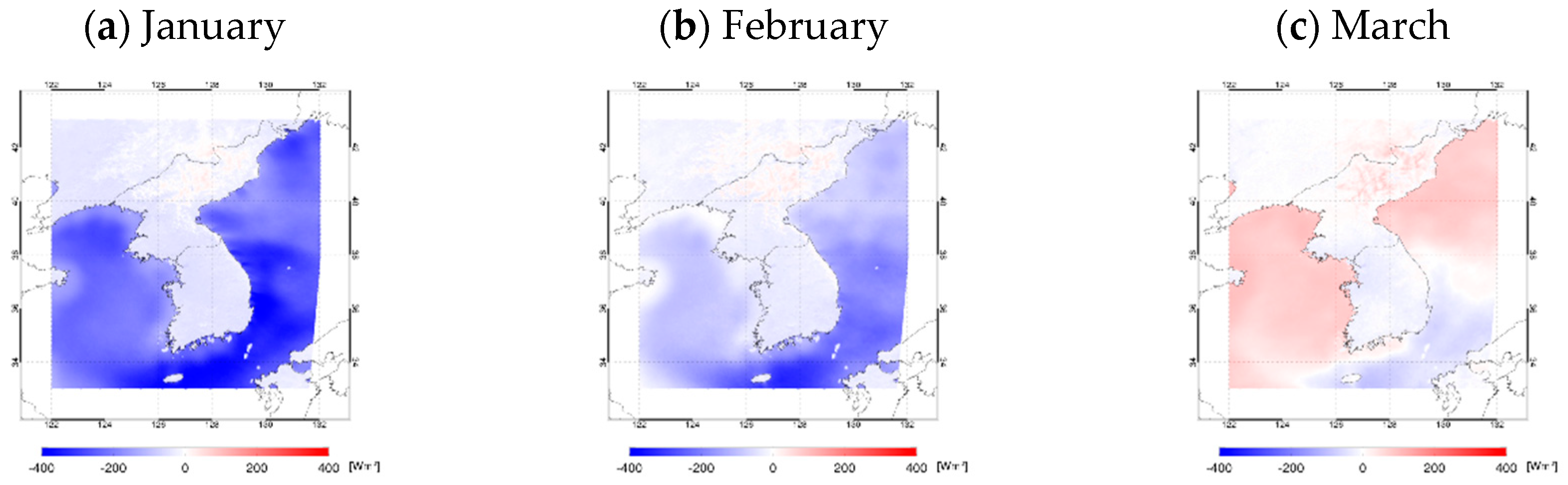
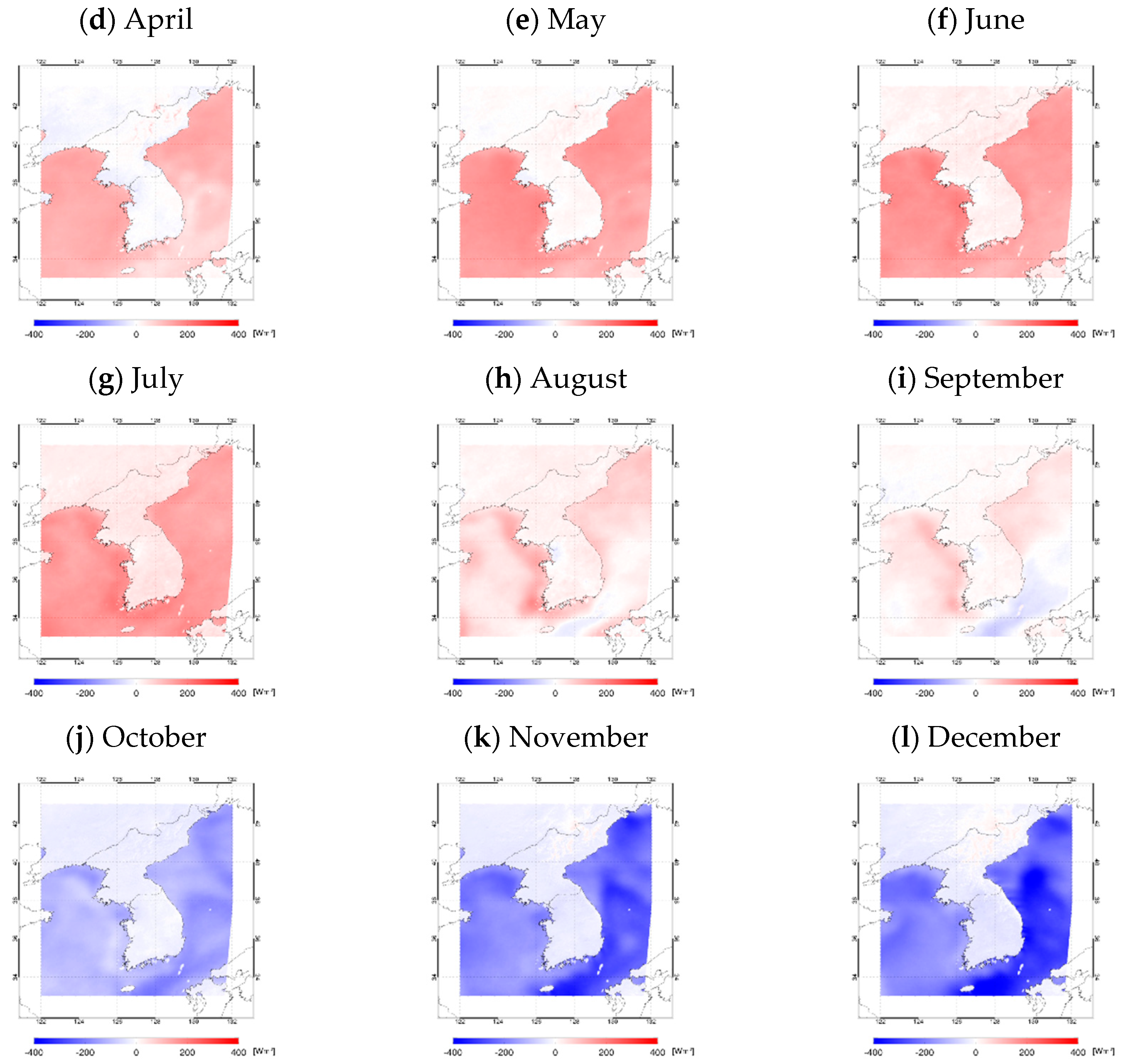
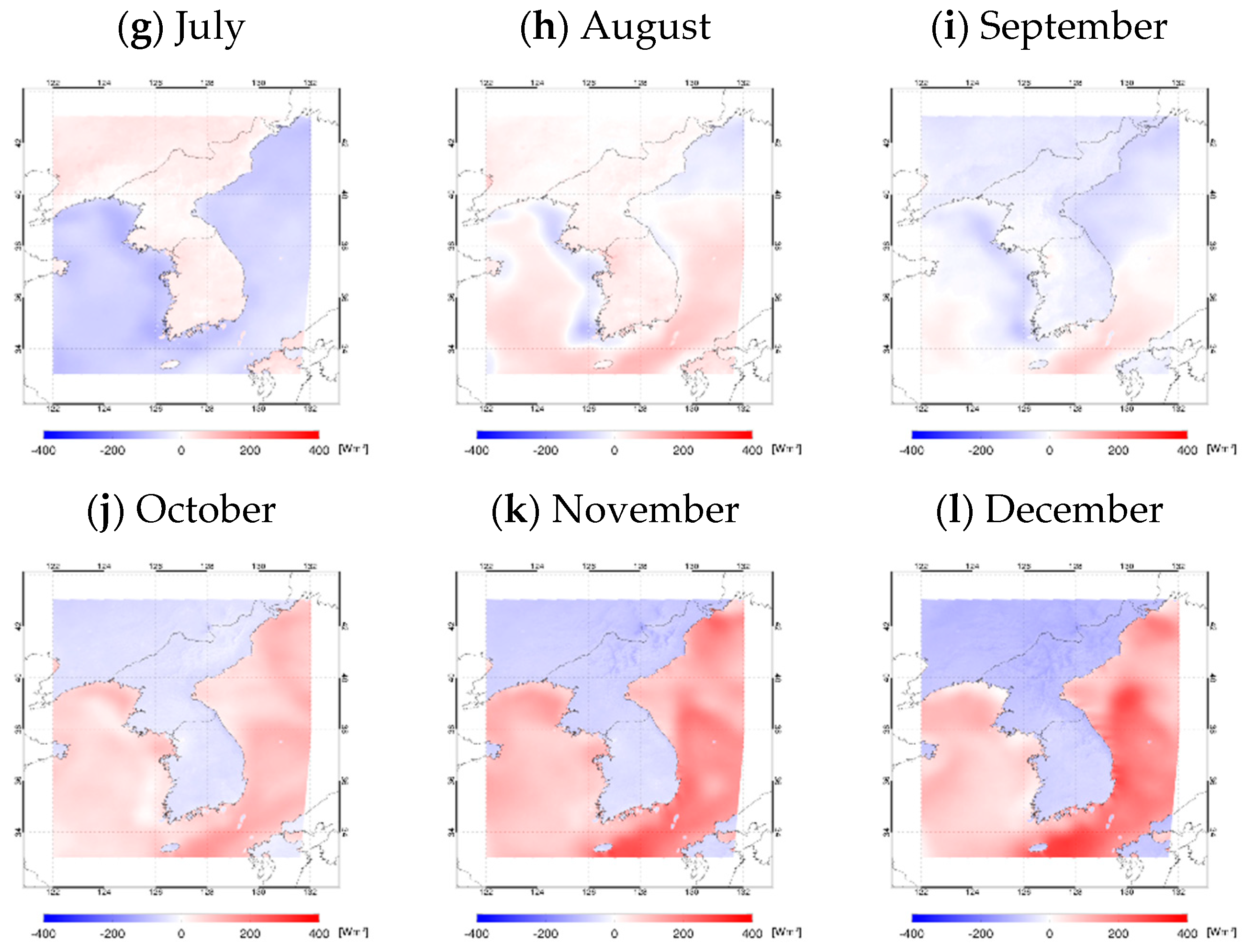
Monthly changes in , , and are shown in Figure 12, Figure 13 and Figure 14. showed a positive net radiation in the spring and summer months, which received high ISR, and it showed a negative net radiation in fall and winter (Figure 12). Similar to , showed a positive net radiation in spring and summer and a negative net radiation in fall and winter (Figure 13). In the South Sea and East Sea regions, SHF+LHF increased during spring and winter under the effect of the Kuroshio current, and thus a strong negative net radiation was observed. Figure 14 shows the distribution of through the difference between and . During spring and summer, land areas, which showed a relatively high temperature distribution, had positive net radiation; and during fall and winter, sea areas had a positive net radiation.
4.3. Regional Energy Budgets within the Korean Peninsula
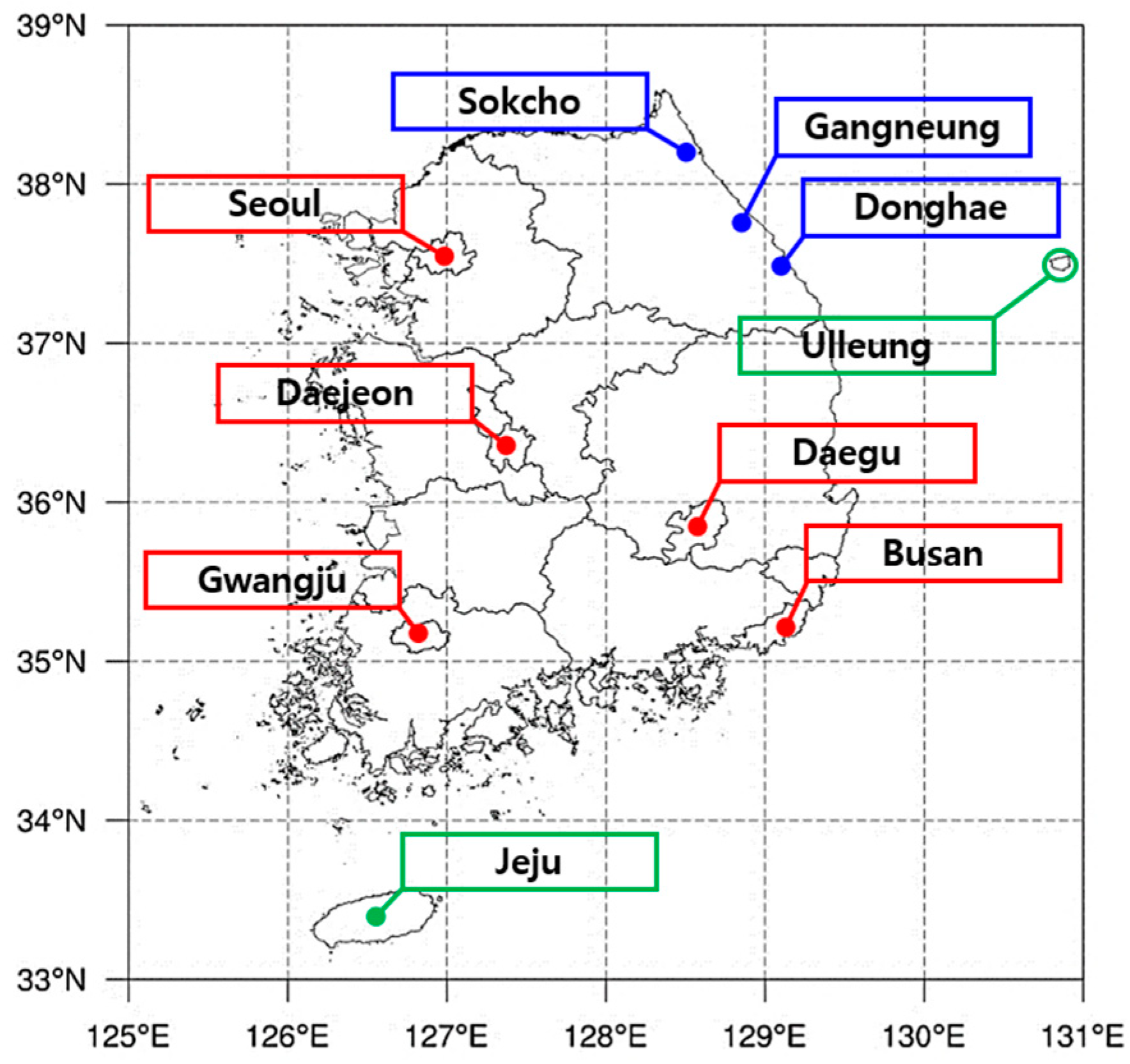
At the scale of a country such as South Korea, the energy budget of the Korean Peninsula region showed different regional characteristics. In particular, the emission and absorption of / varied among metropolises and areas outside of them. In metropolitan regions such as Seoul, the surface temperature was high and the temperature changes were large due to the high heat capacity of man-made structures and the heat island effect; thus, / showed a negative/positive net radiation (emission/absorption) [90,91]. Regions such as Gangneung lie adjacent to the Taebaek Mountains (refer to Figure 1) on the west side and the ocean on the east side, which form complex weather conditions, and the cold air of northeasterly winds flows in from the air masses of the Okhotsk Sea, lowering the temperature and reducing temperature changes; thus, / showed a positive/negative net radiation (absorption/emission). In order to analyze such regional differences, the Korean Peninsula was divided into the metropolitan regions (red) of Seoul, Busan, Daegu, Daejeon, and Gwangju; three regions on the left side of the Taebaek Mountains (the Yeongdong region in blue) including Gangneung, the East Sea, and Sokcho; and the island regions (green) of Jeju and Ulleung, as shown in Figure 15. With this classification, the mean energy budget corresponding to the area of each city was found and used in the analysis.
The energy budget for each city is shown as , , and in Figure 16. The distribution of was similar in all cities, but island regions had a relatively large amount of cloud cover compared to other regions (the Korean Peninsula mean is approximately 45.2%, and the island region mean is approximately 52.4%). Consequently, there was a large radiation of RSR (the Korean Peninsula mean was approximately 113.1 Wm−2, and the island region mean was approximately 123.2 Wm−2), and was smaller than that of the Korean Peninsula monthly mean (Table 12). In the Ulleung region, the mean cloud cover was small in May and June at 20.7% and 34.9%, respectively, and thus the value was high. The Yeongdong region is located at a higher latitude than other regions, and thus its ISR was smaller (the Korean Peninsula mean was approximately 341.4 Wm−2, and the Yeongdong region mean was approximately 335.7 Wm−2). Therefore, was smaller than that of the Korean Peninsula mean (Table 12). Figure 16b shows the distribution, which, unlike , showed clear regional characteristics. was smaller than the mean of the Korean Peninsula in metropolitan regions, similar to the mean in island regions and larger than the mean in the Yeongdong region. Metropolitan regions emitted more energy than other regions because the surface temperatures were high (metropolitan region mean: 288.3 K, Yeongdong region mean: 285.5 K, island region mean: 286.9 K). The variations in surface temperature were small in the island and Yeongdong regions due to the effects of the ocean, and they had a similar or larger mean than the Korean Peninsula. In particular, the Yeongdong region absorbed approximately 21.1 Wm−2 more energy than the metropolitan regions. The Seoul region (mean surface temperature: 289.5 K), and the Sokcho region (mean surface temperature: 284.7 K) showed the maximum and minimum net radiation with a difference of 38.5 Wm−2 (Table 12). In short, the higher the region’s local surface temperature, the more energy tended to be emitted from the surface, and the lower the region’s surface temperature, the more energy tended to be absorbed.
5. Summary and Conclusions
This study calculated the energy budget for the Korean Peninsula in 2016 as part of research dealing with climate change attributable to changes and imbalances in energy budgets, which are related to the issue of global warming. Satellite data (Himawari-8 AHI) and meteorological data (LDAPS) were used to calculate the energy budget. An algorithm was developed for calculating the shortwave radiation components required to calculate the energy budget such as RSR, DSR, and ASR, as well as longwave radiation components, such as OLR, DLR, and ULR. The calculations were made using an empirical method in which the results of a radiative transfer model and the linear relationship between weather variables were applied. The proposed method does not require surface albedo or emissivity data, which involve high uncertainty. The radiation components were calculated using meteorological data, which have low uncertainty and can easily be acquired/collected. To improve the nonlinearity and accuracy of the calculated radiation components, they were calibrated with CERES broadband radiation, and the results showed a percent bias under 3.5% and a high correlation coefficient of over 0.98 between CERES and calibrated radiation components.
Regarding the calculated energy budget, the Korean Peninsula had an of −2.4 Wm−2 and is located in a region with a relatively balanced energy budget at the top of the atmosphere. With an of −14.5 Wm−2, this region has a large flux of SHF and LHF due to the Kuroshio current and typhoons in the summer and fall. Therefore, energy was emitted outside and within the atmosphere. The energy absorbed in the atmosphere supplied energy to regions with relatively low surface temperatures or transported excess energy to the polar regions such that a global energy budget balance was achieved [7]. Clear differences in energy budgets caused by regional weather and climate characteristics were observed in metropolises and regions outside them. The Seoul region, which has high surface temperatures, showed the highest energy emission (33.4 Wm−2), and the Sokcho region showed energy absorption (5.0 Wm−2). Such differences in local energy budget cause mesoscale energy circulation and affect weather and climate changes [2,3,89]; therefore, continued observation and analysis must be performed to predict future regional climate changes [6,25].
This study used satellite data and NWP data with a high spatiotemporal resolution to analyze energy budgets. In particular, the obtained data are more detailed than those provided by most climate models because the spatiotemporal resolution of the calculated data was 2 km × 2 km at 3-h intervals. Climate change models show large differences in their results according to their input meteorological data and model settings [19]. Furthermore, they have limitations in predicting local climate predictions and contain systematic errors because they provide data with large intervals (e.g., 2.5° × 2.5°) [34]. Therefore, in order to study the local energy budget of a region such as the Korean Peninsula, it is necessary to perform extensive research on using satellite data and performing highly accurate radiation calculations.
Author Contributions
B.-Y.K. led the manuscript writing and contributed to the data analysis and research design. K.-T.L. supervised this study, contributed to the research design and manuscript writing, and served as the corresponding author.
Acknowledgments
This work was supported by “Development of Radiation/Aerosol Algorithms” project, funded by ETRI, which is a subproject of “Development of Geostationary Meteorological Satellite Ground Segment (NMSC−2018-01)” program funded by NMSC (National Meteorological Satellite Center) of KMA (Korea Meteorological Administration).
Conflicts of Interest
The authors declare no conflicts of interest.
Abbreviations
| AHI | Advanced Himawari Imager |
| ASR | Absorbed Shortwave Radiation |
| CERES | Cloud and Earth’s Radiant Energy System |
| DLR | Downward Longwave Radiation |
| DSR | Downward Shortwave Radiation |
| ISR | Incoming Solar Radiation |
| LDAPS | Local Data Assimilation and Prediction System |
| LHF | Latent Heat Flux |
| MERRA-2 | Modern Era Retrospective Analysis for Research and Applications Version 2 |
| OLR | Outgoing Longwave Radiation |
| RSR | Reflected Shortwave Radiation |
| SHF | Sensible Heat Flux |
| ULR | Upward Longwave Radiation |
References
- Houghton, J.T.; Ding, Y.; Griggs, D.J.; Noguer, N.; van der Linden, P.J.; Xiaosu, D.; Maskell, K.; Johnson, C.A. Climate Change 2001: The Scientific Basis; Cambridge University Press: Cambridge, UK, 2001. [Google Scholar]
- Solomon, S. Climate Change 2007: The Physical Science Basis: Working Group I Contribution to the Fourth Assessment Report of the IPCC (Vol. 4); Cambridge University Press: Cambridge, UK, 2007. [Google Scholar]
- Stocker, T. Climate Change 2013: The Physical Science Basis: Working Group I Contribution to the Fifth Assessment Report of the Intergovernmental Panel on Climate Change; Cambridge University Press: Cambridge, UK, 2014. [Google Scholar]
- Lashof, D.A.; Ahuja, D.R. Relative contributions of greenhouse gas emissions to global warming. Nature 1990, 344, 529–531. [Google Scholar] [CrossRef]
- Vitousek, P.M.; Mooney, H.A.; Lubchenco, J.; Melillo, J.M. Human domination of Earth’s ecosystems. Science 1997, 277, 494–499. [Google Scholar] [CrossRef]
- Karl, T.R.; Trenberth, K.E. Modern global climate change. Science 2003, 302, 1719–1723. [Google Scholar] [CrossRef] [PubMed]
- Smith, G.L.; Gibson, G.G.; Harrison, E.F. History of Earth Radiation Budget at Langley Research Center. Available online: https://ams.confex.com/ams/pdfpapers/158948.pdf (accessed on 1 February 2018).
- Walther, G.R.; Post, E.; Convey, P.; Menzel, A.; Parmesan, C.; Beebee, T.J.C.; Fromentin, J.M.; Hoegh-Guldberg, O.; Bairlein, F. Ecological responses to recent climate change. Nature 2002, 416, 389–395. [Google Scholar] [CrossRef] [PubMed]
- Root, T.L.; Price, J.T.; Hall, K.R.; Schneider, S.H. Fingerprints of global warming on wild animals and plants. Nature 2003, 421, 57–60. [Google Scholar] [CrossRef] [PubMed]
- McMichael, A.J.; Woodruff, R.E.; Hales, S. Climate change and human health: Present and future risks. Lancet 2006, 367, 859–869. [Google Scholar] [CrossRef]
- O’Brien, G.; O’Keefe, P.; Rose, J.; Wisner, B. Climate change and disaster management. Disasters 2006, 30, 64–80. [Google Scholar] [CrossRef] [PubMed] [Green Version]
- Bouwer, L.M. Have disaster losses increased due to anthropogenic climate change? Bull. Am. Meteorol. Soc. 2011, 92, 39–46. [Google Scholar] [CrossRef]
- Nordhaus, W.D. Managing the Global Commons: The Economics of Climate Change (Vol. 31); MIT Press: Cambridge, UK, 1994. [Google Scholar]
- Pielke, R.A.; Marland, G.; Betts, R.A.; Chase, T.N.; Eastman, J.L.; Niles, J.O.; Running, S.W. The influence of land-use change and landscape dynamics on the climate system: Relevance to climate-change policy beyond the radiative effect of greenhouse gases. Philos. Trans. R. Soc. Lond. A 2002, 360, 1705–1719. [Google Scholar] [CrossRef] [PubMed]
- Gaffin, S.; Rosenzweig, C.; Parshall, L.; Beattie, D.; Berghage, R.; O’Keeffe, G.; Braman, D. Energy Balance Modeling Applied to a Comparison of White and Green Roof Cooling Efficiency. In Green Roofs in the New York Metropolitan Region Research Report; Columbia University Center for Climate Systems Research and NASA Goddard Institute for Space Studies: New York, NY, USA, 2010. [Google Scholar]
- Sheffield, P.E.; Landrigan, P.J. Global climate change and children’s health: Threats and strategies for prevention. Environ. Health Perspect. 2011, 119, 291–298. [Google Scholar] [CrossRef] [PubMed]
- Coutts, A.M.; Harris, R. A multi-scale assessment of urban heating in Melbourne during an extreme heat event and policy approaches for adaptation. In Melbourne: Victorian Centre for Climate Change and Adaptation Research; Monash University: Clayton, Australia, 2013. [Google Scholar]
- Trenberth, K.E.; Fasullo, J.T.; Kiehl, J. Earth’s global energy budget. Bull. Am. Meteorol. Soc. 2009, 90, 311–323. [Google Scholar] [CrossRef]
- Wild, M.; Folini, D.; Hakuba, M.Z.; Schär, C.; Seneviratne, S.I.; Kato, S.; Rutan, D.; Ammann, C.; Wood, E.F.; König-Langlo, G. The energy balance over land and oceans: An assessment based on direct observations and CMIP5 climate models. Clim. Dyn. 2015, 44, 3393–3429. [Google Scholar] [CrossRef]
- Barkstrom, B.R. The Earth Radiation Budget Experiment (ERBE). Bull. Am. Meteorol. Soc. 1984, 65, 1170–1185. [Google Scholar] [CrossRef] [Green Version]
- Wielicki, B.A.; Barkstrom, B.R.; Harrison, E.F.; Lee, R.B.; Smith, G.L.; Cooper, J.E. Clouds and the Earth’s Radiant Energy System (CERES): An earth observing system experiment. Bull. Am. Meteorol. Soc. 1996, 77, 853–868. [Google Scholar] [CrossRef]
- Wielicki, B.A.; Barkstrom, B.R.; Baum, B.A.; Charlock, T.P.; Green, R.N.; Kratz, D.P.; Lee, R.B.; Minnis, P.; Smith, G.L.; Wong, T.; et al. Clouds and the Earth’s Radiant Energy System (CERES): Algorithm overview. IEEE Trans. Geosci. Remote Sens. 1998, 36, 1127–1141. [Google Scholar] [CrossRef]
- Loeb, N.G.; Priestley, K.J.; Kratz, D.P.; Geier, E.B.; Green, R.N.; Wielicki, B.A.; Hinton, P.O.; Nolan, S.K. Determination of unfiltered radiances from the clouds and the earth’s radiant energy system instrument. J. Appl. Meteorol. 2001, 40, 822–835. [Google Scholar] [CrossRef]
- Kato, S.; Loeb, N.G.; Rose, F.G.; Doelling, D.R.; Rutan, D.A.; Caldwell, T.E.; Yu, L.; Weller, R.A. Surface irradiances consistent with CERES-derived top-of-atmosphere shortwave and longwave irradiances. J. Clim. 2013, 26, 2719–2740. [Google Scholar] [CrossRef]
- L’Ecuyer, T.S.; Beaudoing, H.K.; Rodell, M.; Olson, W.; Lin, B.; Kato, S.; Clayson, C.A.; Wood, E.; Sheffield, J.; Adler, R.; et al. The observed state of the energy budget in the early twenty-first century. J. Clim. 2015, 28, 8319–8346. [Google Scholar] [CrossRef]
- Matthews, G. In-flight spectral characterization and calibration stability estimates for the clouds and the earth’s radiant energy system (CERES). J. Atmos. Ocean. Technol. 2009, 26, 1685–1716. [Google Scholar] [CrossRef]
- Ma, Q.; Wang, K.; Wild, M. Impact of geolocations of validation data on the evaluation of surface incident shortwave radiation from Earth System Models. J. Geophys. Res. Atmos. 2015, 120, 6825–6844. [Google Scholar] [CrossRef] [Green Version]
- Zhang, X.; Liang, S.; Wild, M.; Jiang, B. Analysis of surface incident shortwave radiation from four satellite products. Remote Sens. Environ. 2015, 165, 186–202. [Google Scholar] [CrossRef]
- Zhang, X.; Liang, S.; Wang, G.; Yao, Y.; Jiang, B.; Cheng, J. Evaluation of the reanalysis surface incident shortwave radiation products from NCEP, ECMWF, GSFC, and JMA using satellite and surface observations. Remote Sens. 2016, 8, 225. [Google Scholar] [CrossRef]
- Ramanathan, V. The role of earth radiation budget studies in climate and general circulation research. J. Geophys. Res. Atmos. 1987, 92, 4075–4095. [Google Scholar] [CrossRef]
- Kiehl, J.T.; Trenberth, K.E. Earth’s annual global mean energy budget. Bull. Am. Meteorol. Soc. 1997, 78, 197–208. [Google Scholar] [CrossRef]
- Loeb, N.G.; Wielicki, B.A.; Doelling, D.R.; Smith, G.L.; Keyes, D.F.; Kato, S.; Manalo-Smith, N.; Wong, T. Toward optimal closure of the Earth’s top-of-atmosphere radiation budget. J. Clim. 2009, 22, 748–766. [Google Scholar] [CrossRef]
- Wild, M.; Folini, D.; Schär, C.; Loeb, N.; Dutton, E.G.; König-Langlo, G. The global energy balance from a surface perspective. Clim. Dyn. 2013, 40, 3107–3134. [Google Scholar] [CrossRef]
- Jakob Themeßl, M.; Gobiet, A.; Leuprecht, A. Empirical-statistical downscaling and error correction of daily precipitation from regional climate models. Int. J. Climatol. 2011, 31, 1530–1544. [Google Scholar] [CrossRef]
- Bessho, K.; Date, K.; Hayashi, M.; Ikeda, A.; Imai, T.; Inoue, H.; Kumagai, Y.; Miyakawa, T.; Murata, H.; Ohno, T.; et al. An introduction to Himawari-8/9-Japan’s new-generation geostationary meteorological satellites. J. Meteorol. Soc. Jpn. Ser. II 2016, 94, 151–183. [Google Scholar] [CrossRef]
- Park, J.H.; Bok, J.Y.; Han-Oh, H.S.L.; Chung, D.W. Development of Radiometric Calibration System for GEO-KOMPSAT-2 AMI. In Proceedings of the SpaceOps 2016 Conference, Daejeon, Korea, 16–20 May 2016; Available online: https://0-doi-org.brum.beds.ac.uk/10.2514/6.2016-2325 (accessed on 1 February 2018).
- Murata, H.; Takahashi, M.; Kosaka, Y. VIS and IR bands of Himawari-8/AHI compatible with those of MTSAT-2/Imager. MSC Tech. Note 2015, 60, 1–18. [Google Scholar]
- Cullen, M.J.P. The unified forecast/climate model. Meteorol. Mag. 1993, 122, 81–94. [Google Scholar]
- Berrisford, P.; Dee, D.P.; Poli, P.; Brugge, R.; Fielding, K.; Fuentes, M.; Kållberg, P.W.; Kobayashi, S.; Uppala, S.; Simmons, A. The ERA-Interim Archive Version 2.0; ERA Report Series 1; ECMWF: Reading, UK, 2011. [Google Scholar]
- KMA. Climatological Normal of Korea (1981–2010). 2011. Available online: http://www.weather.go.kr/down/Climatological_2010.pdf (accessed on 21 June 2018).
- KMA. Annual Climatological Report (2016). 2016. Available online: http://www.weather.go.kr/repositary/sfc/pdf/sfc_ann_2016.pdf (accessed on 21 June 2018).
- NASA. CERES SYN1deg Ed3A Data Quality Summary. 2013. Available online: https://ceres.larc.nasa.gov/documents/DQ_summaries/CERES_SYN1deg_Ed3A_DQS.pdf (accessed on 1 February 2018).
- Loeb, N.G.; Lyman, J.M.; Johnson, G.C.; Allan, R.P.; Doelling, D.R.; Wong, T.; Soden, B.J.; Stephens, G.L. Observed changes in top-of-the-atmosphere radiation and upper-ocean heating consistent within uncertainty. Nat. Geosci. 2012, 5. [Google Scholar] [CrossRef]
- NASA. CERES EBAF Ed4.0 Data Quality Summary. 2017. Available online: https://ceres.larc.nasa.gov/documents/DQ_summaries/CERES_EBAF_Ed2.8_DQS.pdf (accessed on 1 February 2018).
- NASA. MERRA-2: File Specification. 2016. Available online: https://gmao.gsfc.nasa.gov/pubs/docs/Bosilovich785.pdf (accessed on 1 February 2018).
- NASA. MERRA-2 Input Observations: Summary and Assessment. 2016. Available online: https://gmao.gsfc.nasa.gov/pubs/docs/McCarty885.pdf (accessed on 1 February 2018).
- Bosilovich, M.G.; Robertson, F.R.; Chen, J. Global energy and water budgets in MERRA. J. Clim. 2011, 24, 5721–5739. [Google Scholar] [CrossRef]
- Gelaro, R.; McCarty, W.; Suárez, M.J.; Todling, R.; Molod, A.; Takacs, L.; Randles, C.A.; Darmenov, A.; Bosilovich, M.G.; Reichle, R.; et al. The modern-era retrospective analysis for research and applications, version 2 (MERRA-2). J. Clim. 2017, 30, 5419–5454. [Google Scholar] [CrossRef]
- Dee, D.P.; Källén, E.; Simmons, A.J.; Haimberger, L. Comments on “Reanalyses suitable for characterizing long-term trends”. Bull. Am. Meteorol. Soc. 2011, 92, 65–70. [Google Scholar] [CrossRef]
- Spencer, J.W. Fourier series representation of the position of the sun. Search 1971, 2, 172. [Google Scholar]
- Prsa, A.; Harmanec, P.; Torres, G.; Mamajek, E.; Asplund, M.; Capitaine, N.; Christensen-Dalsgaard, J.; Depagne, E.; Haberreiter, M.; Hekker, S.; et al. Nominal values for selected solar and planetary quantities: IAU 2015 Resolution B3. Astron. J. 2016, 152. [Google Scholar] [CrossRef]
- Lee, S.H.; Kim, B.Y.; Lee, K.T.; Zo, I.S.; Jung, H.S.; Rim, S.H. Retrieval of reflected shortwave radiation at the top of the atmosphere using Himawari-8/AHI data. Remote Sens. 2018, 10, 213. [Google Scholar] [CrossRef]
- Loeb, N.G.; Hinton, P.O.R.; Green, R.N. Top-of-atmosphere albedo estimation from angular distribution models: A comparison between two approaches. J. Geophys. Res. Atmos. 1999, 104, 31255–31260. [Google Scholar] [CrossRef] [Green Version]
- Kato, S.; Marshak, A. Solar zenith and viewing geometry–dependent errors in satellite retrieved cloud optical thickness: Marine stratocumulus case. J. Geophys. Res. Atmos. 2009, 114. [Google Scholar] [CrossRef]
- Ricchiazzi, P.; Yang, S.; Gautier, C.; Sowle, D. SBDART: A research and teaching software tool for plane-parallel radiative transfer in the earth’s atmosphere. Bull. Am. Meteorol. Soc. 1998, 79, 2101–2114. [Google Scholar] [CrossRef]
- Clerbaux, N.; Dewitte, S.; Gonzalez, L.; Bertrand, C.; Nicula, B.; Ipe, A. Outgoing longwave flux estimation: Improvement of angular modelling using spectral information. Remote Sens. Environ. 2003, 85, 389–395. [Google Scholar] [CrossRef]
- Bisht, G.; Venturini, V.; Islam, S.; Jiang, L.E. Estimation of the net radiation using MODIS (Moderate Resolution Imaging Spectroradiometer) data for clear sky days. Remote Sens. Environ. 2005, 97, 52–67. [Google Scholar] [CrossRef]
- Kato, S.; Loeb, N.G.; Rutan, D.A.; Rose, F.G.; Sun-Mack, S.; Miller, W.F.; Chen, Y. Uncertainty estimate of surface irradiances computed with MODIS-, CALIPSO-, and CloudSat-derived cloud and aerosol properties. Surv. Geophys. 2012, 33, 395–412. [Google Scholar] [CrossRef]
- Li, Z.Q.; Leighton, H.G.; Masuda, K.; Takashima, T. Estimation of SW flux absorbed at the surface from TOA reflected flux. J. Clim. 1993, 6, 317–330. [Google Scholar] [CrossRef]
- NOAA. GOES-R Advanced Baseline Imager (ABI) Algorithm Theoretical Basis Document for Absorbed Shortwave Radiation (Surface). 2010. Available online: http://www.goes-r.gov/products/ATBDs/option2/RB_ASR_v1.0_no_color.pdf (accessed on 1 February 2018).
- Ohring, G.; Gruber, A.; Ellingson, R. Satellite determinations of the relationship between total longwave radiation flux and infrared window radiance. J. Clim. Appl. Meteorol. 1984, 23, 416–425. [Google Scholar] [CrossRef]
- Abel, P.G.; Gruber, A. An improved model for the calculation of longwave flux at 11 μm. In NOAA Technical Memorandum NESS 106; National Oceanic and Atmospheric Administration: Washington, DC, USA, 1979. [Google Scholar]
- Schmetz, J.; Liu, Q. Outgoing longwave radiation and its diurnal variation at regional scales derived from Meteosat. J. Geophys. Res. Atmos. 1988, 93, 11192–11204. [Google Scholar] [CrossRef]
- Otterman, J.; Starr, D.; Brakke, T.; Davies, R.; Jacobowitz, H.; Mehta, A.; Cheruy, F.; Prabhakara, C. Modeling zenith-angle dependence of outgoing longwave radiation: Implication for flux measurements. Remote Sens. Environ. 1997, 62, 90–100. [Google Scholar] [CrossRef]
- Kim, B.Y.; Lee, K.T.; Jee, J.B.; Zo, I.S. Retrieval of outgoing longwave radiation at top-of-atmosphere using Himawari-8 AHI data. Remote Sens. Environ. 2018, 204, 498–508. [Google Scholar] [CrossRef]
- Swinbank, W.C. Long-wave radiation from clear skies. Q. J. R. Meteorol. Soc. 1963, 89, 339–348. [Google Scholar] [CrossRef]
- Idso, S.B.; Jackson, R.D. Thermal radiation from the atmosphere. J. Geophys. Res. 1969, 74, 5397–5403. [Google Scholar] [CrossRef]
- Brutsaert, W. Evaporation into the Atmosphere: Theory, History and Applications; Kluwer Academic Publishers: Dordrecht, The Netherlands, 1982. [Google Scholar]
- Heitor, A.; Biga, A.J.; Rosa, R. Thermal radiation components of the energy balance at the ground. Agric. For. Meteorol. 1991, 54, 29–48. [Google Scholar] [CrossRef]
- Santos, C.A.C.D.; Silva, B.B.D.; Rao, T.V.R.; Satyamurty, P.; Manzi, A.O. Downward longwave radiation estimates for clear-sky conditions over northeast Brazil. Rev. Br. Meteorol. 2011, 26, 443–450. [Google Scholar] [CrossRef]
- Iziomon, M.G.; Mayer, H.; Matzarakis, A. Downward atmospheric longwave irradiance under clear and cloudy skies: Measurement and parameterization. J. Atmos. Sol. Terr. Phys. 2003, 65, 1107–1116. [Google Scholar] [CrossRef]
- Lee, H.T.; Laszlo, I.; Gruber, A. ABI earth radiation budget-downward longwave radiation: Surface (DLR). In NOAA Nesdis Center for Satellite Applications and Research Algorithm Theoretical Basis Document; National Oceanic and Atmospheric Administration: Washington, DC, USA, 2010. [Google Scholar]
- Sobrino, J.A.; El Kharraz, J.; Li, Z.L. Surface temperature and water vapour retrieval from MODIS data. Int. J. Remote Sens. 2003, 24, 5161–5182. [Google Scholar] [CrossRef]
- Jin, M.; Liang, S. An improved land surface emissivity parameter for land surface models using global remote sensing observations. J. Clim. 2006, 19, 2867–2881. [Google Scholar] [CrossRef]
- Doelling, D.R.; Loeb, N.G.; Keyes, D.F.; Nordeen, M.L.; Morstad, D.; Nguyen, C.; Wielicki, B.A.; Young, D.F.; Sun, M. Geostationary enhanced temporal interpolation for CERES flux products. J. Atmos. Ocean. Technol. 2013, 30, 1072–1090. [Google Scholar] [CrossRef]
- Doelling, D.R.; Sun, M.; Nguyen, L.T.; Nordeen, M.L.; Haney, C.O.; Keyes, D.F.; Mlynczak, P.E. Advances in geostationary-derived longwave fluxes for the CERES synoptic (SYN1deg) Product. J. Atmos. Ocean. Technol. 2016, 33, 503–521. [Google Scholar] [CrossRef]
- Yu, L.; Weller, R.A. Objectively analyzed air-sea heat fluxes for the global ice-free oceans (1981–2005). Bull. Am. Meteorol. Soc. 2007, 88, 527–539. [Google Scholar] [CrossRef]
- Roberts, J.B.; Clayson, C.A.; Robertson, F.R.; Jackson, D.L. Predicting near-surface atmospheric variables from Special Sensor Microwave/Imager using neural networks with a first-guess approach. J. Geophys. Res. Atmos. 2010, 115. [Google Scholar] [CrossRef] [Green Version]
- Garratt, J.R. The atmospheric boundary layer. Earth Sci. Rev. 1994, 37, 89–134. [Google Scholar] [CrossRef]
- Stull, R.B. An Introduction to Boundary Layer Meteorology (Vol. 13); Springer Science & Business Media: Berlin, Germany, 2012. [Google Scholar]
- Hansen, J.; Nazarenko, L.; Ruedy, R.; Sato, M.; Willis, J.; Del Genio, A.; Koch, D.; Lacis, A.; Lo, K.; Menon, S.; et al. Earth’s energy imbalance: Confirmation and implications. Science 2005, 308, 1431–1435. [Google Scholar] [CrossRef] [PubMed]
- Kim, D.; Ramanathan, V. Solar radiation budget and radiative forcing due to aerosols and clouds. J. Geophys. Res. Atmos. 2008, 113. [Google Scholar] [CrossRef] [Green Version]
- Zo, I.S.; Jee, J.B.; Kim, B.Y.; Lee, K.T. Baseline Surface Radiation Network (BSRN) quality control of solar radiation data on the Gangneung-Wonju National University radiation station. Asia Pac. J. Atmos. Sci. 2017, 53, 11–19. [Google Scholar] [CrossRef]
- Hansen, J.; Sato, M.; Kharecha, P.; Schuckmann, K.V. Earth’s energy imbalance and implications. Atmos. Chem. Phys. 2011, 11, 13421–13449. [Google Scholar] [CrossRef] [Green Version]
- Trenberth, K.E. An imperative for climate change planning: Tracking Earth’s global energy. Curr. Opin. Environ. Sustain. 2009, 1, 19–27. [Google Scholar] [CrossRef]
- Fasullo, J.T.; Trenberth, K.E. The annual cycle of the energy budget. Part II: Meridional structures and poleward transports. J. Clim. 2008, 21, 2313–2325. [Google Scholar] [CrossRef]
- Yu, L. Global variations in oceanic evaporation (1958–2005): The role of the changing wind speed. J. Clim. 2007, 20, 5376–5390. [Google Scholar] [CrossRef]
- Fasullo, J.T.; Trenberth, K.E. The annual cycle of the energy budget. Part I: Global mean and land-ocean exchanges. J. Clim. 2008, 21, 2297–2312. [Google Scholar] [CrossRef]
- Inagaki, A.; Letzel, M.O.; Raasch, S.; Kanda, M. Impact of surface heterogeneity on energy imbalance: A study using LES. J. Meteorol. Soc. Jpn. Ser. II 2006, 84, 187–198. [Google Scholar] [CrossRef]
- Shepherd, J.M.; Pierce, H.; Negri, A.J. Rainfall modification by major urban areas: Observations from spaceborne rain radar on the TRMM satellite. J. Appl. Meteorol. 2002, 41, 689–701. [Google Scholar] [CrossRef]
- Zehnder, J.A. Simple modifications to improve fifth-generation Pennsylvania State University-National Center for Atmospheric Research mesoscale model performance for the Phoenix, Arizona, metropolitan area. J. Appl. Meteorol. 2002, 41, 971–979. [Google Scholar] [CrossRef]
Figure 1.
Korean Peninsula region (red box) and altitude distribution for energy budget calculation.
Figure 1.
Korean Peninsula region (red box) and altitude distribution for energy budget calculation.

Figure 2.
Scatter plot of calculated DLR (red: calibrated result in this study, blue: [71] method) and CERES DLR.
Figure 2.
Scatter plot of calculated DLR (red: calibrated result in this study, blue: [71] method) and CERES DLR.

Figure 3.
Scatter plot of infrared atmospheric transmittance according to surface temperature and OLR.
Figure 3.
Scatter plot of infrared atmospheric transmittance according to surface temperature and OLR.

Figure 4.
Density scatter plot of calculated shortwave radiation components and CERES shortwave radiation before (a,c,e) and after (b,d,f) calibration. Here, N is the total number of samples used for verification. The black dash line is the 1:1 line and the red line is the regression line. The unit of RMSE is Wm−2.


Figure 5.
Density scatter plot of calculated longwave radiation components and CERES longwave radiation before (a,c,e) and after (b,d,f) calibration. Here, N is the total number of samples used for verification. The black dash line is the 1:1 line and the red line is the regression line. The unit of RMSE is Wm−2.


Figure 6.
Daily mean (a) SHF and (b) LHF of MERRA-2 and LDAPS in 2016 before and after calibration.

Figure 7.
Daily mean time series distribution of CERES and calculated (a) ISR; (b) RSR; (c) DSR; and (d) ASR.
Figure 7.
Daily mean time series distribution of CERES and calculated (a) ISR; (b) RSR; (c) DSR; and (d) ASR.


Figure 8.
Daily mean time series distribution of CERES and calculated (a) OLR; (b) DLR; and (c) ULR.
Figure 8.
Daily mean time series distribution of CERES and calculated (a) OLR; (b) DLR; and (c) ULR.


Figure 9.
Daily mean time series distribution of GWNU observatory, CERES, and calculated (a) DSR and (b) DLR. Observation at GWNU observatory are missing in Julian day 108–110 and 295–301.
Figure 9.
Daily mean time series distribution of GWNU observatory, CERES, and calculated (a) DSR and (b) DLR. Observation at GWNU observatory are missing in Julian day 108–110 and 295–301.

Figure 10.
Annual mean radiation components and energy budget of the Korean Peninsula region in 2016. Red: Radiation components and energy budget calculated using CERES and MERRA-2 data (values in parentheses are the results of analyzing only 350 days of data used in this study); Blue: radiation components and energy budget calculated in this study.

Figure 11.
Annual mean energy budget for 2016 at (a) the top of the atmosphere; (b) the surface; and (c) in the atmosphere; and (d) surface temperature distribution.
Figure 11.
Annual mean energy budget for 2016 at (a) the top of the atmosphere; (b) the surface; and (c) in the atmosphere; and (d) surface temperature distribution.

Figure 12.
Distribution of monthly mean energy budget () at the top of the atmosphere for the Korean Peninsula region in 2016.
Figure 12.
Distribution of monthly mean energy budget () at the top of the atmosphere for the Korean Peninsula region in 2016.

Figure 13.
Distribution of monthly mean energy budget () at the surface for the Korean Peninsula region in 2016.
Figure 13.
Distribution of monthly mean energy budget () at the surface for the Korean Peninsula region in 2016.


Figure 14.
Distribution of monthly mean energy budget () in the atmosphere for the Korean Peninsula region in 2016.
Figure 14.
Distribution of monthly mean energy budget () in the atmosphere for the Korean Peninsula region in 2016.


Figure 15.
Metropolitan, Yeongdong, and island region cities for studying energy budgets by region in the Korean Peninsula.
Figure 15.
Metropolitan, Yeongdong, and island region cities for studying energy budgets by region in the Korean Peninsula.

Figure 16.
Monthly mean energy budget time series for the Korean Peninsula and cities by region in 2016 at (a) the top of the atmosphere; (b) the surface; and (c) in the atmosphere.
Figure 16.
Monthly mean energy budget time series for the Korean Peninsula and cities by region in 2016 at (a) the top of the atmosphere; (b) the surface; and (c) in the atmosphere.


Table 1.
Settings of the radiative transfer model for calculating the broadband albedo at the top of the atmosphere
Table 1.
Settings of the radiative transfer model for calculating the broadband albedo at the top of the atmosphere
| Parameter | Values | N |
|---|---|---|
| Spectral Band (μm) | 0.41–0.51, 0.47–0.55, 0.56–0.71, 0.81–0.91, 1.55–1.67, 2.19–2.32, 0.2–3.3 | 7 |
| Atmospheric Profile | Tropical, Mid-Latitude Summer & Winter, Sub-Arctic Summer & Winter, US Standard | 6 |
| SZA (°) | 0, 5, 10, 15, 20, 25, 30, 35, 40, 45, 50, 55, 60, 65, 70, 75, 80, 85 | 18 |
| RAA (°) | 0, 10, 20, 30, 40, 50, 60, 70, 80, 90, 100, 110, 120, 130, 140, 150, 160, 170, 180 | 19 |
| Aerosol Optical Thickness (AOT) | Rural, Urban, Oceanic, Tropospheric: VIS 1, 5, 10, 15, 20 km | 20 |
| Cloud Optical Thickness (COT) | 2, 4, 8, 16, 32, 64, 128 | 7 |
| Cloud Height (km) | 2, 4, 6, 8, 10, 12, 14, 16 | 8 |
| Surface Albedo | 0.0, 1.0, Water (spectral range mean: 0.04), Vegetation (0.28), Sand (0.32), Snow (0.43) | 6 |
Table 2.
Settings of the radiative transfer model for calculating DSR and ASR
| Parameter | Values | N |
|---|---|---|
| Spectral Band (μm) | 0.2–3.3 | 1 |
| Atmospheric Profile | Tropical, Mid-Latitude Summer & Winter, Sub-Arctic Summer & Winter, US Standard | 6 |
| CSZA | 0.1, 0.2, 0.3, 0.4, 0.5, 0.6, 0.7, 0.8, 0.9, 1.0 | 10 |
| TPW (cm) | 0.2, 0.4, 0.8, 1.6, 3.2, 6.4 | 6 |
| AOT | Rural, Urban, Oceanic, Tropospheric: 0.02, 0.04, 0.08, 0.16, 0.32, 0.64, 1.28 | 28 |
| COT | 2, 4, 8, 16, 32, 64, 128 | 7 |
| Cloud Height (km) | 2, 4, 6, 8, 10, 12, 14, 16 | 8 |
| Cloud Effective Radius (μm) | Water Cloud: 8, 16, 32, 64 Ice Cloud: 16, 32, 64, 128 | 8 |
| Surface Albedo | 0.0, 1.0, Water (0.04), Vegetation (0.28), Sand (0.32), Snow (0.43) | 6 |
Table 3.
Regression coefficients for calculating DSR and ASR
| DSR | ||||||
| ASR | ||||||
Table 4.
Settings of the radiative transfer model for calculating OLR
| Parameter | Values | N |
|---|---|---|
| Spectral Band (μm) | 5.44–7.03, 11.18–13.65, 3.3–100 | 3 |
| Atmospheric Profile | Tropical, Mid-Latitude Summer & Winter, Sub-Arctic Summer & Winter, US Standard | 6 |
| SZA (°) | 0, 5, 10, 15, 20, 25, 30, 35, 40, 45, 50, 55, 60, 65, 70, 75, 80, 85 | 18 |
| COT | 2, 4, 8, 16, 32, 64, 128 | 7 |
| Cloud Height (km) | 0, 2, 4, 6, 8, 10, 12, 14, 16 | 9 |
| Temperature, H2O, CO2, O3, etc. | Default |
Table 5.
Regression coefficients of each channel for converting radiance into irradiance
| Channel | ||||||
|---|---|---|---|---|---|---|
| 8 | ||||||
| 15 |
Table 6.
Regression coefficients for converting narrowband irradiance to OLR
Table 7.
Regression coefficients for calculating DLR.
Table 8.
Regression coefficients for calculating ULR.
Table 9.
CERES example used in the verification of each calculated radiation component and observation time
Table 9.
CERES example used in the verification of each calculated radiation component and observation time
| Shortwave Radiation (RSR, DSR, ASR) | Longwave Radiation (OLR, DLR, ULR) | |||
|---|---|---|---|---|
| Month | Day | Time | Day | Time |
| 1 | 4, 20 | 0230 UTC | 4, 20 | 0230, 1330 UTC |
| 2 | 5, - | 5, - | ||
| 3 | 8, 24 | 8, 24 | ||
| 4 | 2, - | 2, 18 | ||
| 5 | 4, 20 | 4, 20 | ||
| 6 | 5, - | 5, 21 | ||
| 7 | 7, 23 | 7, 23 | ||
| 8 | 6, 22 | 6, 22 | ||
| 9 | 7, 23 | 7, 23 | ||
| 10 | 2, 18 | 2, 18 | ||
| 11 | 3, 19 | 3, 19 | ||
| 12 | 5, 21 | 5 *, 21 | ||
* Excluded from analysis because Himawari-8 AHI data at 0230 UTC were missing. - Missing case.
Table 10.
Bias, RMSE and correlation coefficient (R) of CERES and calculated radiation components using 2016 daily mean data. The mean, bias, and RMSE units are Wm−2.
Table 10.
Bias, RMSE and correlation coefficient (R) of CERES and calculated radiation components using 2016 daily mean data. The mean, bias, and RMSE units are Wm−2.
| CERES Mean | Bias | RMSE | R | |
|---|---|---|---|---|
| ISR | ||||
| RSR | ||||
| DSR | ||||
| ASR | ||||
| OLR | ||||
| DLR | ||||
| ULR |
Table 11.
Bias, RMSE, and correlation coefficient (R) of DSR and DLR observed at the GWNU observatory and CERES and calculated DSR and DLR. The mean, bias, and RMSE units are Wm−2.
Table 11.
Bias, RMSE, and correlation coefficient (R) of DSR and DLR observed at the GWNU observatory and CERES and calculated DSR and DLR. The mean, bias, and RMSE units are Wm−2.
| Observation Mean | Bias | RMSE | R | ||
|---|---|---|---|---|---|
| DSR | CERES | ||||
| Calculation | |||||
| DLR | CERES | ||||
| Calculation |
Table 12.
Energy budgets for the Korean Peninsula, metropolitan, Yeongdong, and island regions at the top of the atmosphere (), the surface (), and the atmosphere () (unit: Wm−2).
Table 12.
Energy budgets for the Korean Peninsula, metropolitan, Yeongdong, and island regions at the top of the atmosphere (), the surface (), and the atmosphere () (unit: Wm−2).
| Korean Peninsula | Metropolitan | Yeongdong | Island | |
|---|---|---|---|---|
(Seoul: ) | (Sokcho: ) | |||
(Seoul: ) | (Sokcho: ) |
© 2018 by the authors. Licensee MDPI, Basel, Switzerland. This article is an open access article distributed under the terms and conditions of the Creative Commons Attribution (CC BY) license (http://creativecommons.org/licenses/by/4.0/).
Share and Cite
MDPI and ACS Style
Kim, B.-Y.; Lee, K.-T. Radiation Component Calculation and Energy Budget Analysis for the Korean Peninsula Region. Remote Sens. 2018, 10, 1147. https://0-doi-org.brum.beds.ac.uk/10.3390/rs10071147
AMA Style
Kim B-Y, Lee K-T. Radiation Component Calculation and Energy Budget Analysis for the Korean Peninsula Region. Remote Sensing. 2018; 10(7):1147. https://0-doi-org.brum.beds.ac.uk/10.3390/rs10071147
Chicago/Turabian StyleKim, Bu-Yo, and Kyu-Tae Lee. 2018. "Radiation Component Calculation and Energy Budget Analysis for the Korean Peninsula Region" Remote Sensing 10, no. 7: 1147. https://0-doi-org.brum.beds.ac.uk/10.3390/rs10071147
Note that from the first issue of 2016, this journal uses article numbers instead of page numbers. See further details here.