Large-Scale Accurate Reconstruction of Buildings Employing Point Clouds Generated from UAV Imagery


1
Faculty of Geodesy and Geomatics Engineering, Khaje Nasir Toosi University of Technology, 19667-15433 Tehran, Iran
2
Institute of Geodesy and Photogrammetry, Technical University of Braunschweig, 38106 Braunschweig, Germany
3
Faculty of Geomatics, Computer Science and Mathematics, University of Applied Sciences, 70174 Stuttgart, Germany
*
Author to whom correspondence should be addressed.
Remote Sens. 2018, 10(7), 1148; https://0-doi-org.brum.beds.ac.uk/10.3390/rs10071148
Submission received: 27 May 2018
/
Revised: 9 July 2018
/
Accepted: 16 July 2018
/
Published: 20 July 2018
(This article belongs to the Special Issue 3D Reconstruction & Semantic Information from Aerial and Satellite Images)
Abstract
:High-density point clouds are valuable and detailed sources of data for different processes related to photogrammetry. We explore the knowledge-based generation of accurate large-scale three-dimensional (3D) models of buildings employing point clouds derived from UAV-based photogrammetry. A new two-level segmentation approach based on efficient RANdom SAmple Consensus (RANSAC) shape detection is developed to segment potential facades and roofs of the buildings and extract their footprints. In the first level, the cylinder primitive is implemented to trim point clouds and split buildings, and the second level of the segmentation produces planar segments. The efficient RANSAC algorithm is enhanced in sizing up the segments via point-based analyses for both levels of segmentation. Then, planar modelling is carried out employing contextual knowledge through a new constrained least squares method. New evaluation criteria are proposed based on conceptual knowledge. They can examine the abilities of the approach in reconstruction of footprints, 3D models, and planar segments in addition to detection of over/under segmentation. Evaluation of the 3D models proves that the geometrical accuracy of LoD3 is achieved, since the average horizontal and vertical accuracy of the reconstructed vertices of roofs and footprints are better than (0.24, 0.23) m, (0.19, 0.17) m for the first dataset, and (0.35, 0.37) m, (0.28, 0.24) m for the second dataset.
1. Introduction
Three-dimensional (3D) city models have been in demand since the mid-1990s for various applications such as photorealistic real-time visualization of terrestrial walkthroughs [1]. More recently, it has become widespread through the internet in such applications as Google Earth [1]. One of the significant entities of 3D city model is building, which includes roof and walls with various structures. These features can be modelled in different details. The City Geography Markup Language (CityGML) is an Open Geospatial Consortium (OGC) interoperable data model and encoding standard for demonstrating city models. According to CityGML version 2.0, there are five levels of detail (LoD) for its building module. The architectural model of a building is represented by a geometrically exact outer shell in LoD3 [2]. Each LoD should enforce a minimum horizontal and vertical accuracy [2], and thus LoD3 should observe a specific accuracy, which is 0.5 m horizontally and vertically. This model can be employed in Building Information Modelling (BIM) [3] and evacuation scenarios [4].
3D building reconstruction can be characterized by the approach taken, the data used, the target feature which should be reconstructed, and assumptions of modelling, which are discussed in the following.
Reconstruction can most broadly be classified as bottom-up/data-driven and top-down/model-driven. In data-driven approaches, the building is divided into individual elements, which are reconstructed directly from the geometric information of the data. In model-driven approaches, a reconstruction model is selected from a library as a hypothesis. The data is then used to verify the model [5]. In addition, some researchers use hybrid approaches to benefit from the advantages of both, e.g., [6,7,8]. In [8] cardinal planes of the roof, which include adequate data, were reconstructed through a data-driven method, whereas dormers, which consist of insufficient data, were modelled through a model-driven method. Furthermore, some research such as [6,7] integrate additional knowledge to the data-driven approach in the form of target-based graph matching and feature-driven approach, respectively. In [6] a limited number of common roof shapes as targets and features found in the laser data are matched. Then, the matching is carried out between topological relations among segments with the topology of target objects. In [7] the point cloud is segmented via a sub-surface segmentation method, then a rule-based feature recognition approach detects different sections of the building, next the geometry in each collection of features is adjusted with regard to other features.
A good deal of methodological research is pursued for building reconstruction from different types of data. The most important data sources used in the literature for building reconstruction consist of LIDAR data [9,10,11,12], terrestrial laser scanning data [13], DEM [14], satellite images [15], aerial images [16], images captured by unmanned aerial vehicle (UAV)s [17], image-derived point cloud [18,19,20], building footprint [21], InSAR [22], etc. Each of the aforementioned data types has special characteristics and is most profitable for a part of building reconstruction process and even on occasion in a particular LoD. Furthermore, usually several sources of data, such as DSM and aerial images or LiDAR and optical images, are fused in the reconstruction process [23,24,25,26].
UAVs have advanced capabilities for capturing nadir and oblique images close to the object, which could be applied for coating surfaces of buildings completely [27]. In addition, UAVs can provide images for small urban environments. Therefore, UAV images could be employed for producing dense point clouds for 3D building reconstruction with high details [28]. Dense image matching (DIM) is employed to generate image-derived or so-called photogrammetric point clouds [29]. However, due to occlusions, illumination changes [28], improper viewing angles and ambiguous areas [30] applying DIM to oblique imagery causes different problems. Photogrammetric point clouds usually have versatile spatial distributions [31] and suffer from clutter in depth, because of improper viewing angles and the rapid motion of the platform, plus noisy data on reflective surfaces [32]. Nonetheless, they are cheaper than LiDAR point clouds, especially when they are derived from UAV imagery, and carries texture and color information [31]. Indeed UAVs are fairly inexpensive platforms, also amateur digital cameras, costing a few-hundred euros, can be utilized to produce point clouds with cm-level resolution [33,34]. Furthermore, it is worthy of attention that if this type of point cloud benefits from images with large overlaps and high resolutions, it can be comparable to terrestrial laser scan data, from the viewpoint of quality [28].
Subclasses of the building, which have been reconstructed in 3D city models, are various according to the CityGML standard [35]. Features of interest in semi/full automatically 3D building reconstruction mostly belong to the building’s roof or walls. Additionally, footprint is an essential part in the building reconstruction, in that it indicates the boundary of the building point cloud and separates it from other objects. Generating footprint in [36] is composed of boundary edges identification, tracing edges to form an irregular boundary and boundary regularization. Tracing edge points, collecting collinear points, adjusting the extracted lines and generating footprint are different steps of the proposed method in [37]. Additionally, in some research such as [38], building outline generation is performed via regularization of boundary points of the roof rather than walls, due to the lack of points on walls and neighboring grounds of the building. Moreover, in a wide range of research on wall reconstruction, it was assumed to be vertical. Then, the reconstruction was performed by placing reliance on this assumption and extruding the footprints such as in [38,39,40], to name but a few.
Concerning the aforementioned papers, a new data-driven approach without considering any assumption is applied on the image-derived point cloud. The point cloud is generated from images captured by UAV to produce an accurate 3D model of building and its footprint. One of the important problems in 3D reconstruction with photogrammetric point cloud is its heavy clutter. Moreover, point clouds of the buildings contain different parts, which cannot be of interest in the reconstruction process, and therefore should be removed. Another problem is that working with high-density point clouds is data intensive. In most researches on the metric 3D reconstruction, geometrical accuracy is also a significant parameter. Hence, the processes ought to be managed. To accomplish the aims of the paper, the following contributions are included in this research:
- New data: utilizing high-density photogrammetric point clouds as the only source of data. According to the literature review, most of the papers exploit photogrammetric point clouds as an additional source of data. The capabilities of this type of point cloud in building reconstruction have not been much appreciated.
- Improving segmentation method: point-based analyses are performed to improve the segmentation method in sizing up segments.
- New constrained planar modelling: the modelling method is developed to create models of facades, roofs and the grounds by imposing the constraints on local normal vectors. The plane-based generation of footprints is a novel usage of points on walls and grounds in building reconstruction.
- New evaluation method: this method examines segmentation in the viewpoint of generation of planar segments and proposes vertex-based criteria to explore over/under segmentation and refine the reconstructed footprint.
The following parts of the article are organized to establish the aforementioned items. In Section 2, overview of the proposed approach and background of the research will be explained. In this section, segmentation and the constrained least squares modelling of buildings will be described. In Section 3, data and methods of the research will be discussed. It consists of 2-level segmentation, improvement in the efficient RANSAC algorithm and planar modelling. In Section 4, results of the research and evaluation of segmentation and 3D models will be elaborated. In section 5, discussions are presented. Finally, the most important achievements will be summarized in Section 6.
2. Overview of the Method and Background
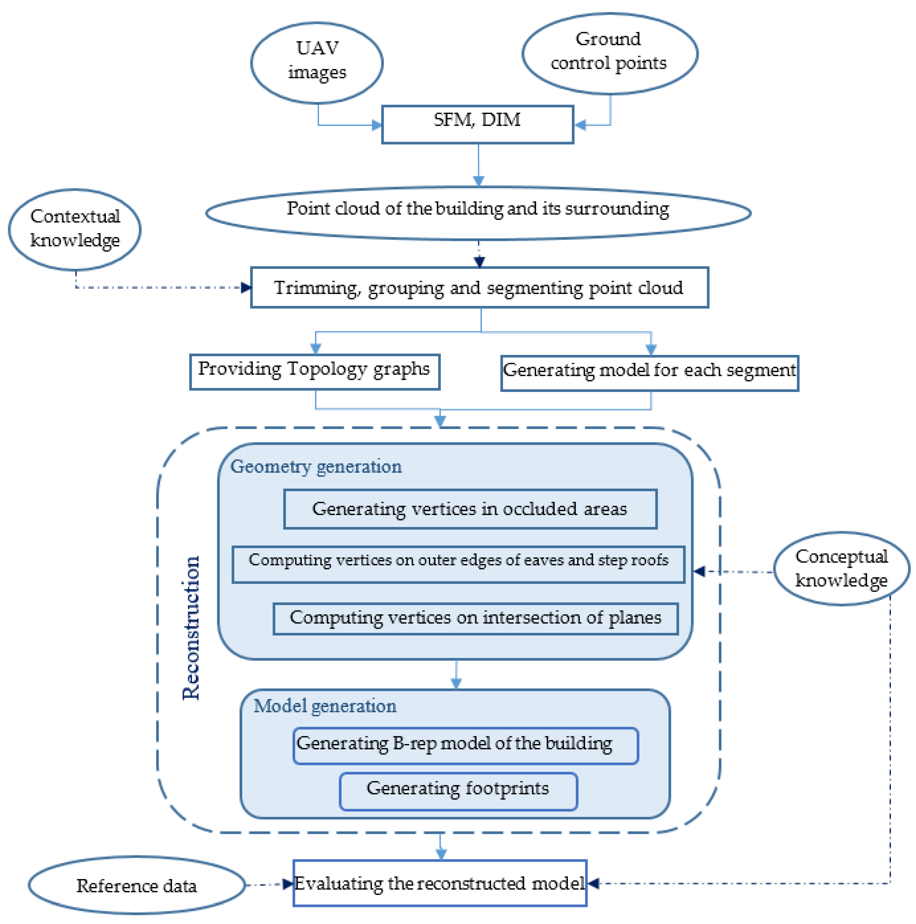
Briefly, this research adopts a RANSAC shape detection method and improves this method, via applying knowledge, to firstly break down high-density point clouds of buildings into smaller sections, and secondly segment them to potential facades and roofs. In addition, point clouds of surrounding grounds of buildings are segmented to generate their footprints. Then, a knowledge-based plane fitting method constructs planar models from segmented patches of point clouds, which are derived from UAV-based photogrammetry. The knowledge is employed to constrain the modelling process in addition to check the reconstructed models. The evaluation step is performed through the new criteria for segmentation and reconstruction. In Figure 1 the workflow of the proposed method is delineated. The details of the method will be explained in Section 3, along with applying the method on data.
2.1. Segmentation
Segmentation is a prominent part of point cloud processing. The objective of this part is to group points into meaningful clusters, whose points have similar characteristics. In [41] segmentation methods were divided into five categories, including edge-based, region-based, attribute-based, graph-based, and model-based. In model-based methods, all points with the same mathematical characteristics are grouped as one segment, e.g., sphere, plane, and cylinder [41].
In [42] a model-based algorithm was proposed to detect basic shapes in unorganized point clouds. Their algorithm is based on RANSAC. This algorithm deals with the shape extraction as an optimization problem utilizing a score function. So that, the primitive with the maximal score is searched using RANSAC. Candidates for all shapes are generated for each minimal subset. The score evaluation scheme counts the number of compatible points for a shape candidate, which constitutes the largest connected component on the shape. The best candidate is selected whenever the probability that no better candidate was overlooked, is high enough. Our research adopts the algorithm proposed in [42], namely the efficient RANSAC, to segment unorganized point clouds of buildings. Because this algorithm yields good results even if a high degree of outlier and noise exists in the point cloud [41]. In addition, it can produce models for the patches of points, which include holes. However, it has deficiency in sizing up the shapes within the point cloud [41].
The efficient RANSAC algorithm uses octree structure and have several parameters including minimum points per primitive to access the optimum sampling, maximum distance of points from primitives, sampling resolution to find connected components, maximum normal deviation of a point from the normal of the sample primitive, and overlooking probability [42]. Optimum sampling is determined in regard to outlier density and distribution and shape size [42]. Overlooking probability relates to the probability of points belonging to each primitive and exhibits the probability of overlooking a better candidate for the shape.
2.2. Constrained Least Squares Modelling
After breaking down point clouds into planar segments, planar models are constructed using the following Equation.
where are coordinates of point and is the unknowns vector of the fitted plane. Furthermore, the angle of the local normal vector with the normal vector of the surface is employed as the constraint through the next Equation.
where . The adjusted planar models for the detected segments are computed via the constrained least squares adjustment (the following Equation), whose initial values for the unknown vector come from the efficient RANSAC.
where is the coefficient matrix, is the unknowns vector, is the observations vector and carries the residuals. In addition, is the constraint matrix and is the constant restriction vector.
One of the presentation method of 3D models is boundary representation (B-rep), which is based on surfaces and consists of two types of information including geometry and topology. Topology graphs of faces are provided and utilized to compute the vertices. Vertices on at least three faces are computed using Cramer’s rule (the next Equation) for solving a system of linear equations with unique solution.
where th column in is replaced with to reach . For the vertices, which are placed on more than three planes, the adjusted coordinates are examined via the weighted average to remove the possible cartographic error due to the existence of several candidates for one corner. The weights are set proportional to the size of the smallest plane in each intersection to generate its candidate.
3. Materials and Methods
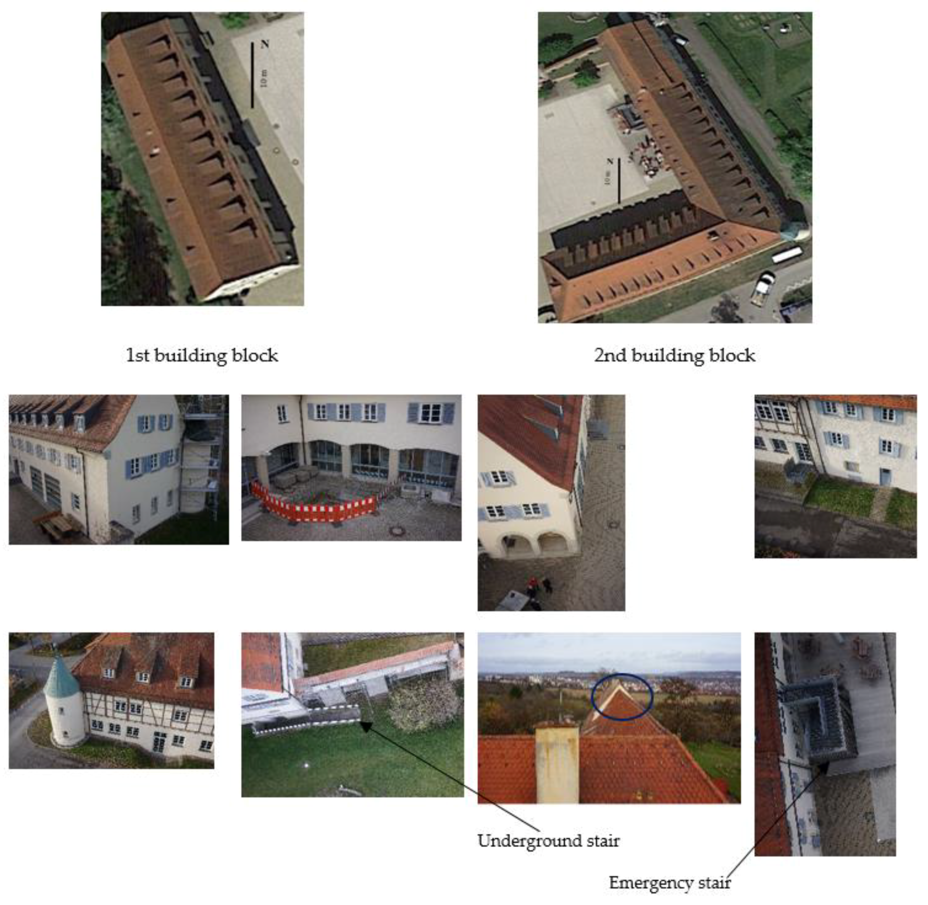
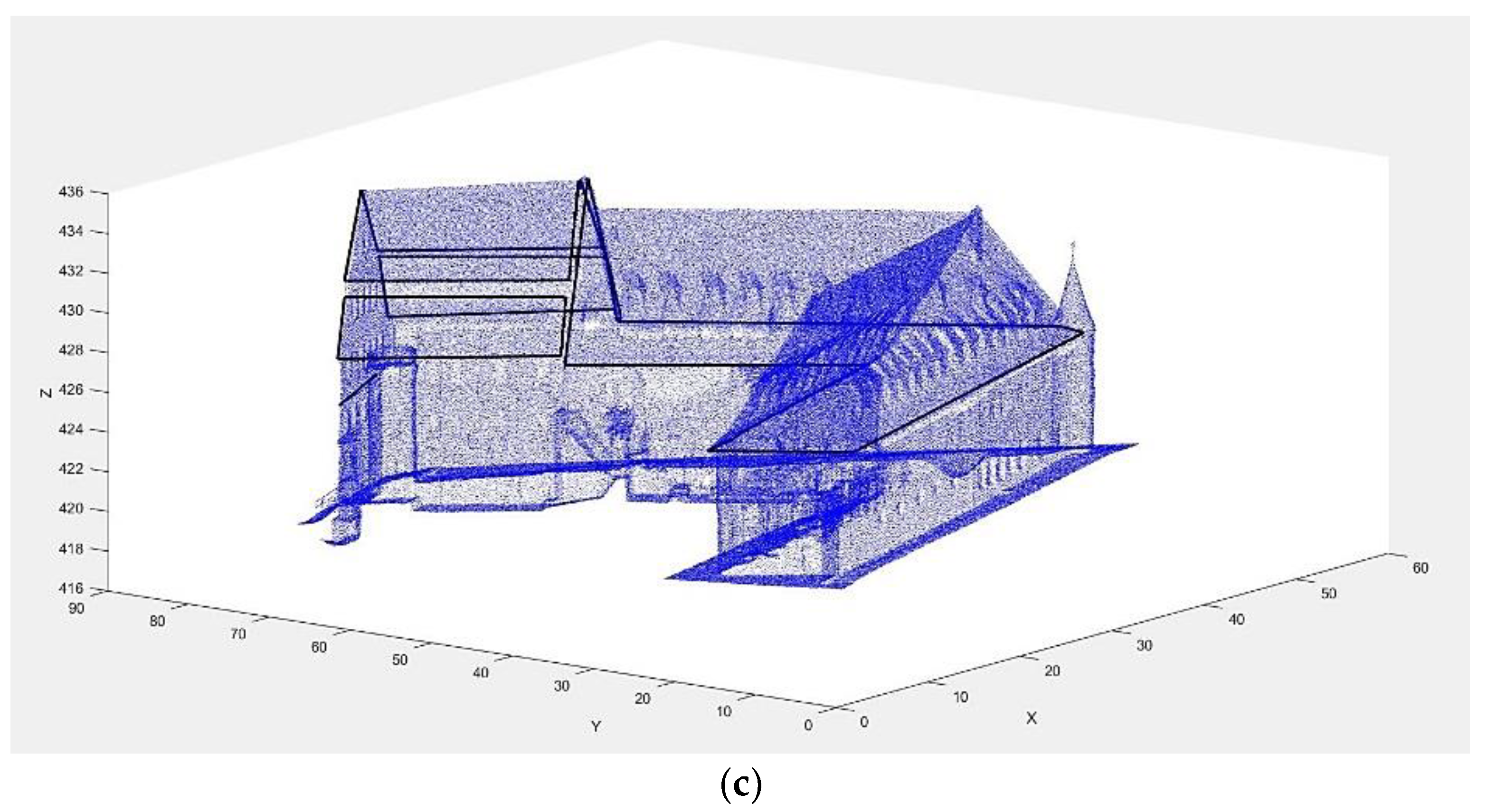
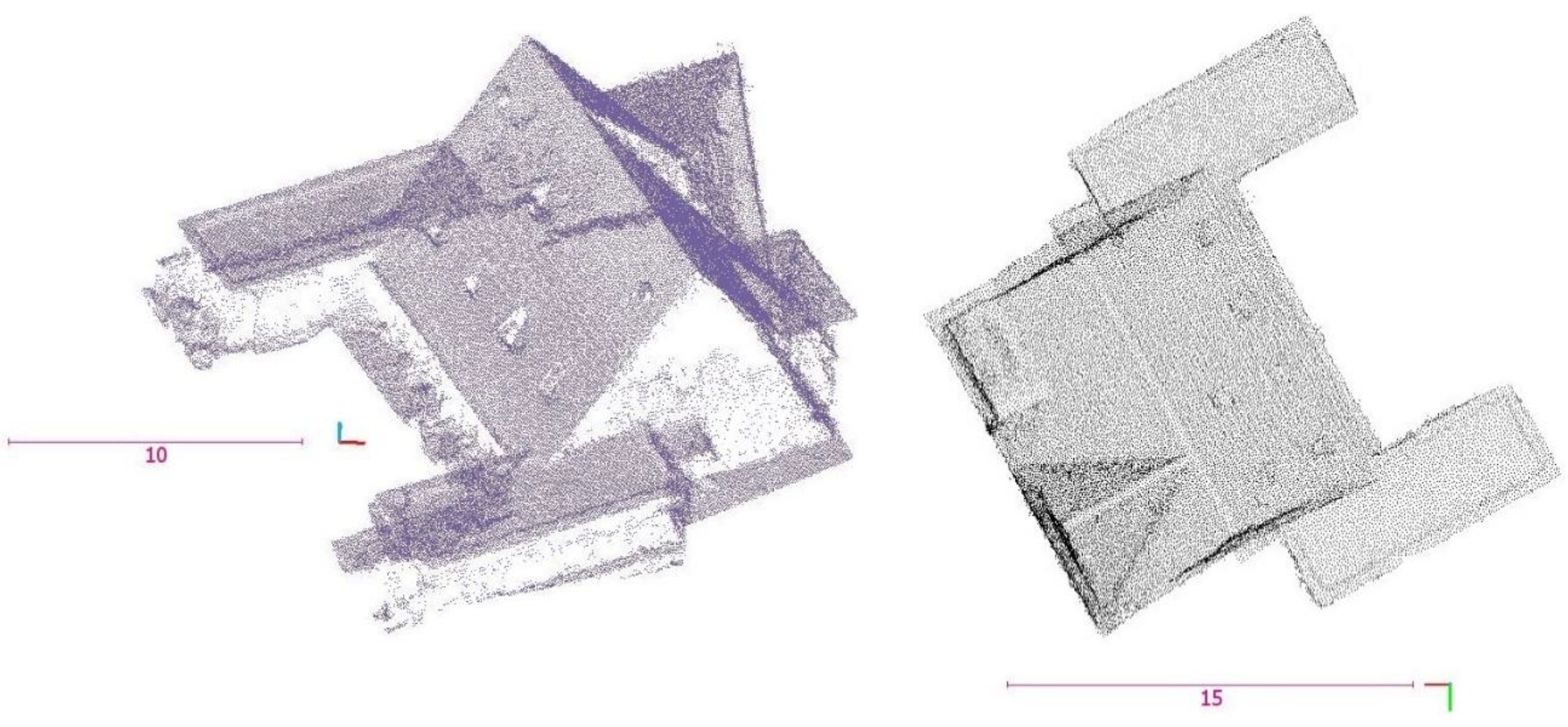
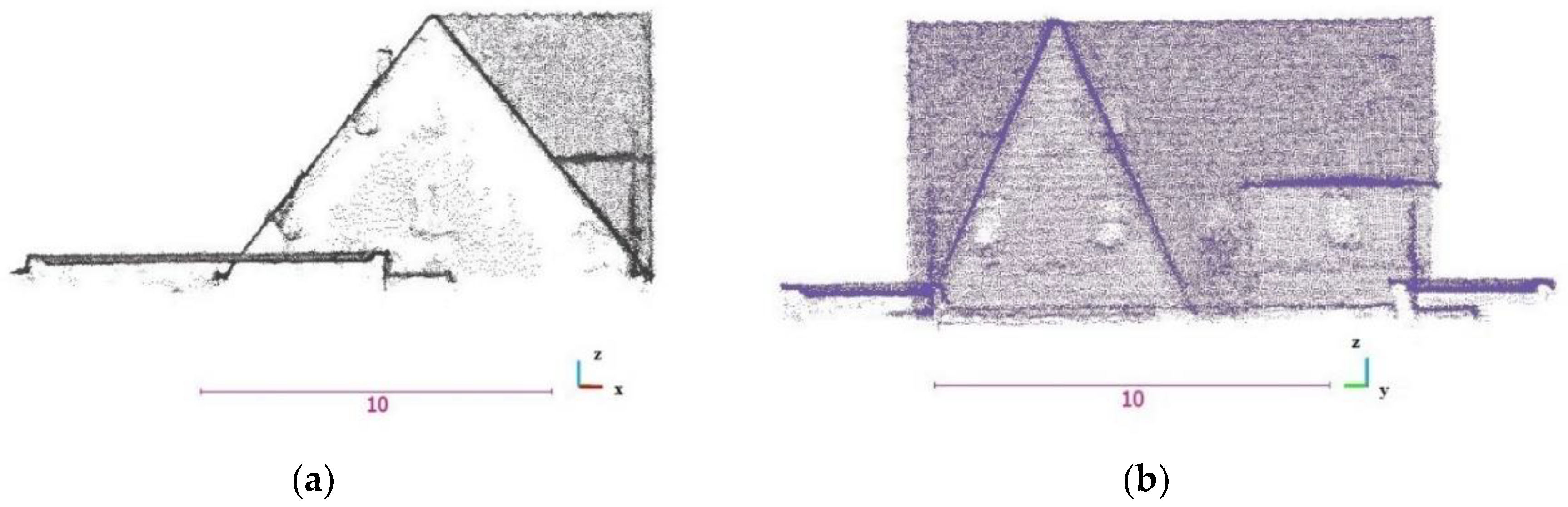
We applied our method on the data, which include two photogrammetric point clouds from different building blocks. These buildings are demonstrated in Figure 2 and are located in Baden-Wuerttemberg, Germany. Both of the datasets include several blocks of connected buildings, which have eaves. Moreover, existence of step roofs in the second building makes the reconstruction process more challenging. The second building is composed of three connected buildings, of which two make L-shaped junction. In addition, both buildings include towers. Scaffolding around the tower of the first building and the walls of the second building, arch holes on the walls of the first building, besides digging part and building materials scattered on the grounds of the second building, plus big and frequent windows on the walls of both buildings, in addition to several stairs around both buildings, all raise challenges of 3D reconstruction process and 3D footprint generation considerably. In Figure 2, some of these details are demonstrated.
In order to generate point clouds, multiview images were captured by a Sony camera with focal length of 35 mm, which was conveyed by a Falcon octocopter. The UAV flew around the entire building and performed nadir and oblique imaging. Details of the flight plan are explained in the following: The average GSD is 1 cm/pixel. In addition, 22 ground control points (GCPs) are prepared and employed for georeferencing and model calculation. The average end lap of the images is 80% and the average side lap is 70%. Moreover, the overall number of the images, which are used in models calculation, are 526. Images were processed with Photoscan software by Agisoft. The self-calibration report of the camera is presented in Appendix A. The sparse point clouds were generated using SFM. Next, dense photogrammetric point clouds were produced via DIM. The average horizontal and vertical errors on 16 GCPs as control points are 0.5 and 1.2 cm, respectively. The average horizontal and vertical errors on 6 check points are 0.7 and 1.5 cm.
Two case studies include about 20 and 53 million points, which spread over areas of 520 m2 and 1240 m2. The average density of the point clouds on roofs is 30 points/dm2. Furthermore, the average density on walls is 20 points/dm2. This amount for grounds is 24 points/dm2.These data are intricate and bear many details, clutter, noises and holes.
3.1. Two-Level Segmentation
According to Section 2.1, the efficient RANSAC algorithm is adopted for the segmentation. At the first stage, the effects of clutter, noise and unwanted parts should be decayed. Then, in order to manage the high volume of data, the point cloud is broken down into several smaller parts. Therefore, the efficient RANSAC is utilized in a new manner.
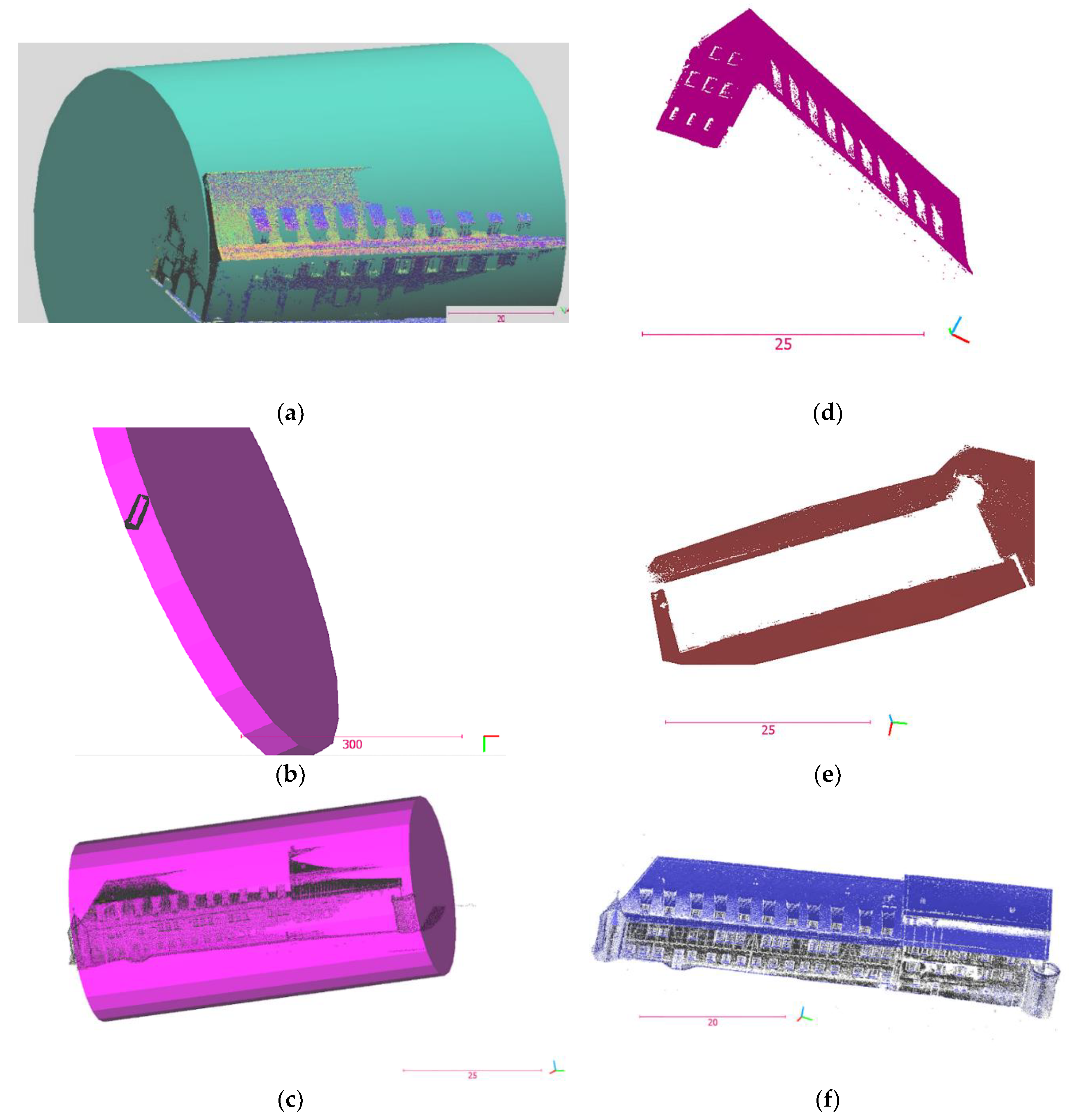
Cylinder is a good candidate to reach the general shape of a rectangle building, because it can be surrounded by the ambient cuboid or surround the encircled cuboid. Based on this idea, buildings are divided via cylinder primitive of the efficient RANSAC (Figure 3a–c). Ranges of the parameters of the algorithm are listed in Table 1. The first two parameters are set to segregate the close points, which are mostly on neighboring patches. The second couple of parameters determine the majority of the compatible points for primitive fitting into patches. The minimum points per primitive is a determining parameter to match sizes of the segments. This item improves the shape detection procedure by localizing sampling and is determined in next section.
Improvement in the Efficient RANSAC
In the first level of segmentation, to overcome the deficiency of the efficient RANSAC in sizing up the shapes, the minimum points per primitive is approximated with the following proposed Equation.
where is the maximum number of clusters. In addition, µ controls the clusters’ sizes concerning the heterogeneity of point clouds and sizes of subsections of the buildings.
In a homogeneous point cloud, a sphere can show local distribution around a point appropriately. Nevertheless, in a heterogeneous point cloud the direction of the highest local distribution around a point is demonstrated by the longest diameter of the ellipsoid of local distribution. The ratio of areas of the cross sections of sphere and ellipsoid with the horizontal plane implies the ratio of their surface densities. Considering the schematic Figure 4a, the ratio of local surface density on an ellipse-shaped and a circle-shaped neighborhood () is calculated via Equation (6), where are the areas of ellipse and circle, respectively with the same number of points. The circle is the unit circle.
Furthermore, are the biggest and the second covariance-based local eigenvalues of point distribution on ellipse. These parameters for the unique circle are 1.
µ is estimated by . In (Figure 4b), the histogram of is displayed. Concerning the histogram, the limits of µ are computed through Equation (7).
where is the bin with the maximum frequency in the histogram. The number of bins () are computed via Rice rule [43]. A number of segmented parts of buildings and footprints are displayed in Figure 3d–f).
In the second level of segmentation, firstly point clouds are filtered using statistical outlier removal filter, proposed in [44]. Secondly, the planar patches are segmented from the point clouds via the efficient RANSAC plane detection. They can be from facades, roof or the grounds and this matter is not determining. Ranges of the parameters of the algorithm are listed in Table 2. The contextual knowledge represents the angles of the bonnet roofs as the maximum tolerance of normal deviation. Sampling resolution starts from the minimum distance between points in the point cloud after the first level of segmentation.
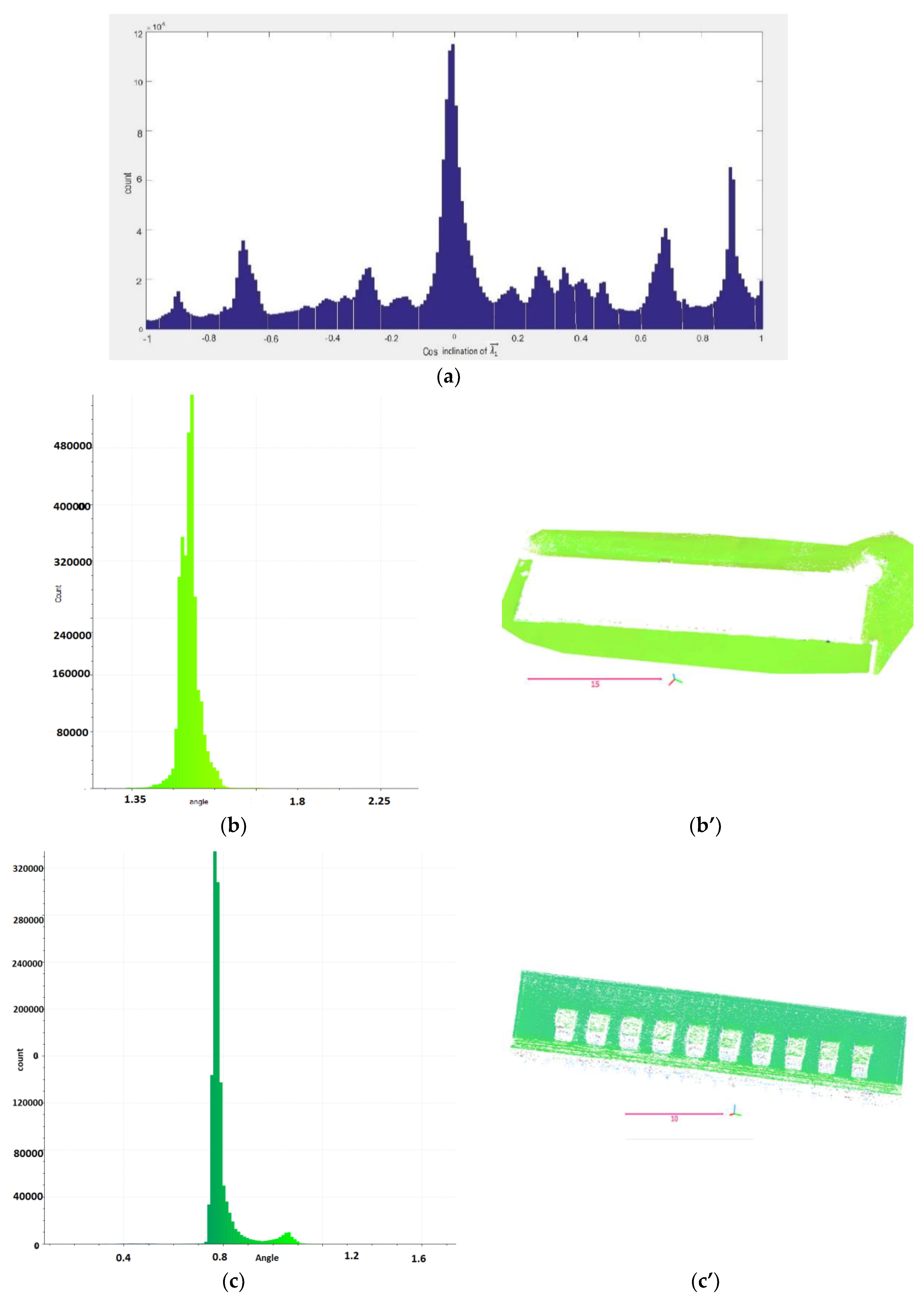
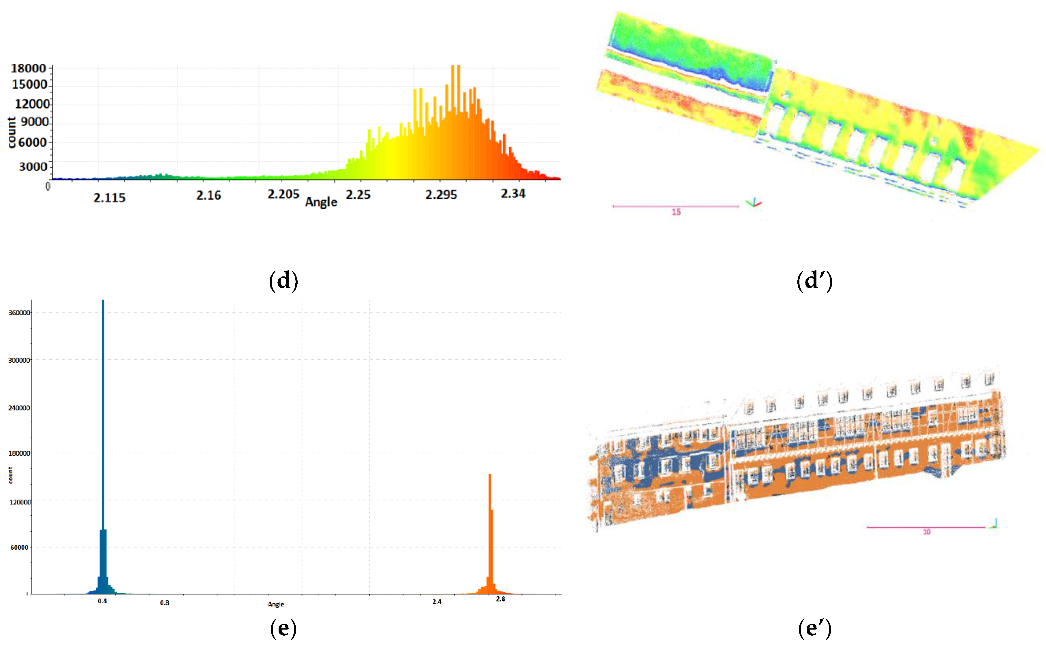
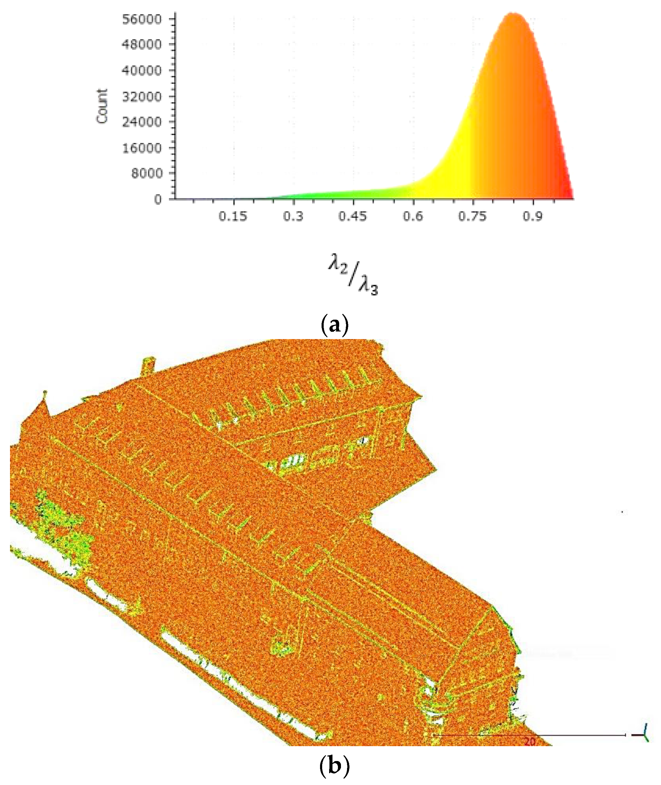
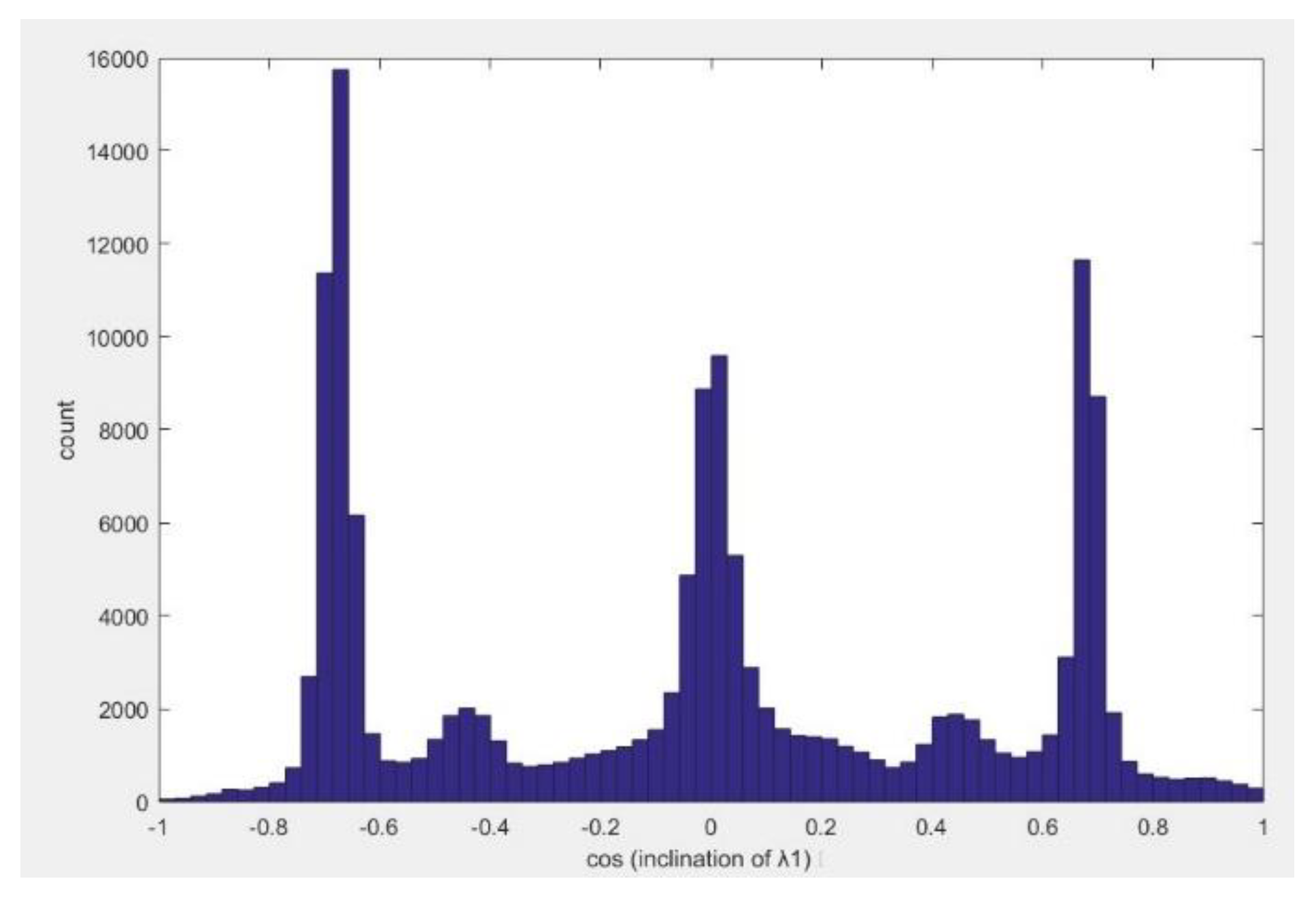
To overcome the drawback of the efficient RANSAC for plane detection, the covariance-based point eigenvectors are computed. These vectors imply the state of local dispersion of points. , the eigenvector which corresponds the smallest eigenvalue, demonstrates the inclination of the underlying surface. Therefore, the histogram of cosine of inclination of roughly shows the number of points on different planar patches () (Figure 5a). As Equation (8) declares, cumulative distribution of the points among every two successive local minima () determines approximate value of the minimum number of points on each planar patch.
In Figure 5b–e histograms of the inclination angle of for several clusters of the footprint, the roof, the step roof and the wall are demonstrated. In Figure 5b’,c’,d’,e’, points in the histograms are marked on the corresponding parts of the clusters with color.
In an iterative approach with a few iterations, the efficient RANSAC algorithm generates shapes of the segmented points with accurate sizes (the following Equation).
In Figure 5d, no sharp peak is displayed on account of the existence of step roofs. In addition, in Figure 5a no differentiation between patches of step roofs is recognizable. In order to approximate the number of points on the step roofs, is computed, where is the largest covariance-based eigenvalue. According to [45], this feature shows significant difference for edges of the borders of half-planes. Therefore, histogram of this feature recognizes the outer edges of the roof (Appendix B Figure A1a,b). Employing the algorithm of line generation discussed in [45], the edges longer than a length tolerance are produced (Appendix B Figure A1c). The directions of these edges correspond to . If any step roof exist in the data, then at least a parallel edge with one of the lowest edge of the roof exists. Thus, the coefficient of is computed via Equation (10), where is the height of the edge.
Then number of points of each section of step roof () derives from . Therefore, is used to compute the parameter of minimum points per primitive in efficient RANSAC algorithm for each parallel part of the step roof via .
The improved method to reconstruct roofs with various horizontal planar patches in different heights is represented in Appendix C. The outcome indicates successful segmentation and reconstruction of horizontal step roofs alongside intersected roof faces.
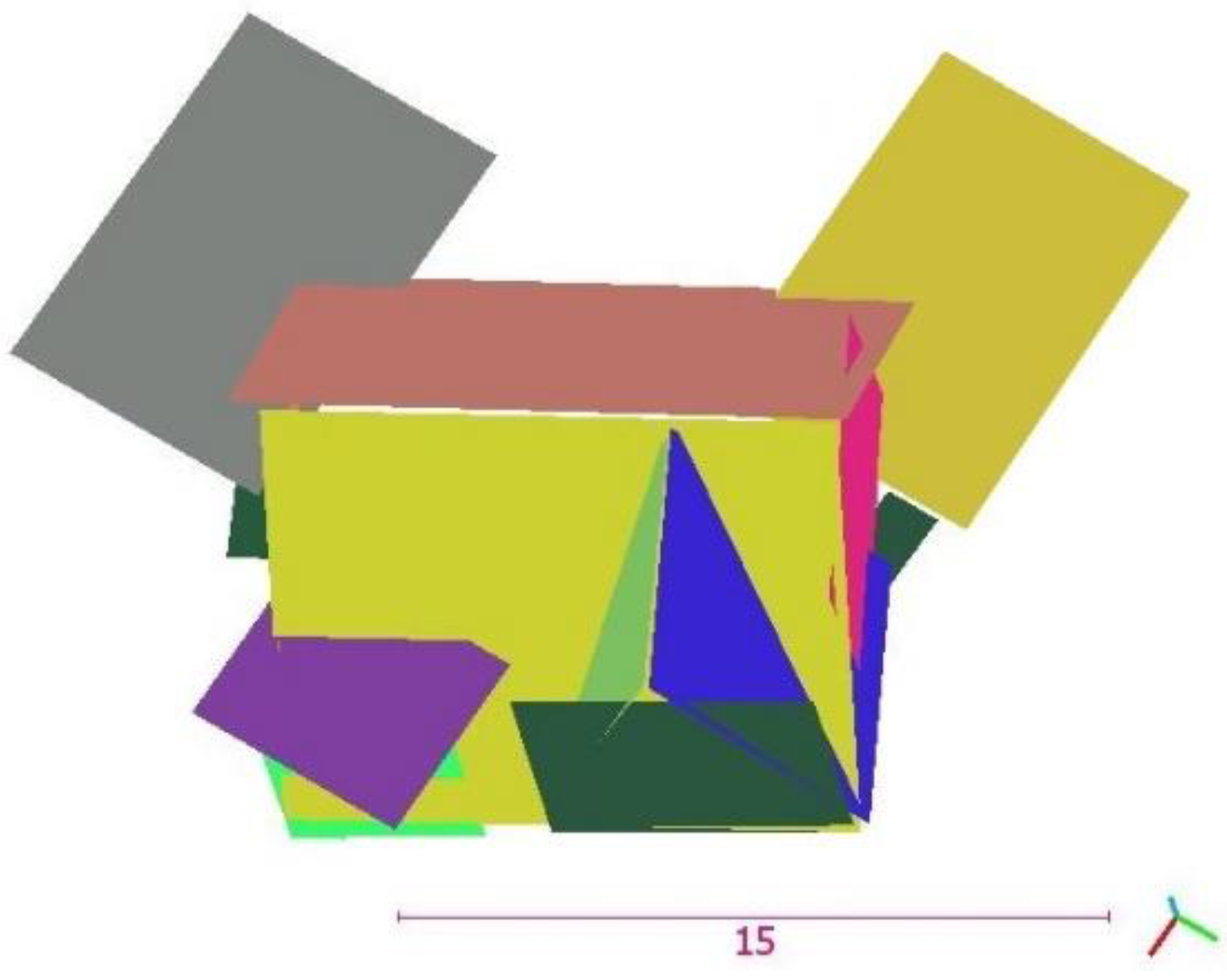
3.2. Planar Modelling
After segmentation, a planar model of each segment is computed via Section 2.2 in MATLAB, in which to keep 95% of all points. This tolerance is set considering deviations of normal vectors in clusters. It is worthy of notice that in order to avoid very big coordinates due to geo-referencing, a global shift was applied on the coordinates. The adjustments show that the highest standard deviation of the constructed planar models of both buildings is less than m.
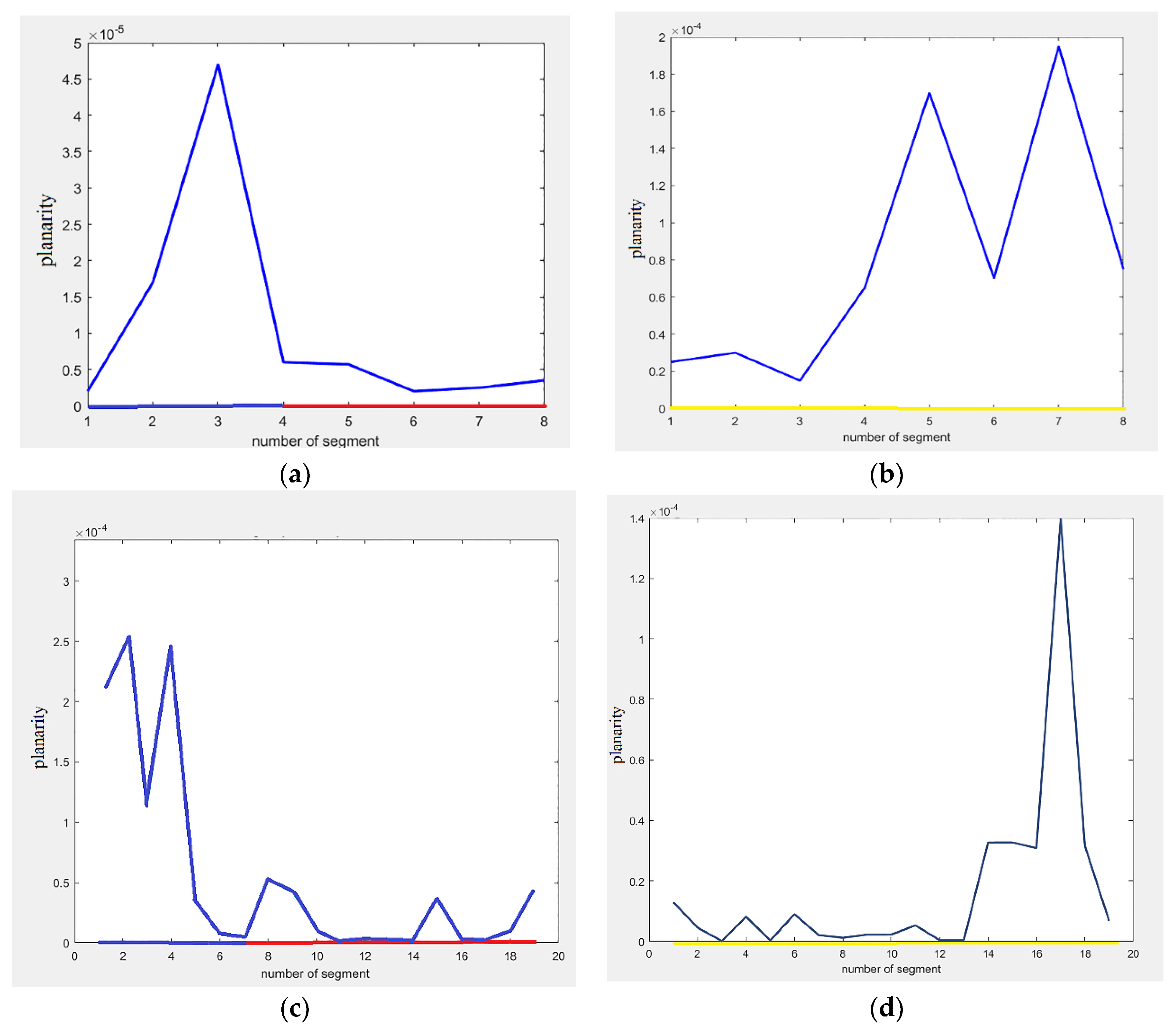
Additionally considering the issue that generation of planar segments is a matter of importance in this research, surface variation is analyzed employing the planarity criteria via Equation (11) [46]. In Figure 6, this parameter is computed for all the extracted segments of roofs, walls and grounds of both datasets.
where are the covariance-based eigenvalues of each segment and is the smallest one. The less the is, the more planar the point cloud of the segment is.
Figure 7 shows the planar models superimposed on the point clouds of building 1 (Figure 7a) and 2 (Figure 7b). In occluded parts, there is no data; therefore, no model is generated in these areas.
In this research, adjacency relations are yielded via convex hulls of the segments, which are computed with PCL (Point Cloud Library) [44]. So that, distances of points of each convex hull are calculated from others’ points. Neighboring convex hulls have at least a number of points with distances shorter than a tolerance, which are set empirically. Then, topology graphs are constituted for two buildings. The vertices of the buildings are computed according to Section 2.2. The outer vertices of the eaves and step roofs are generated through the regularized convex hulls, which are created by the conceptual knowledge about shapes of the faces. It is worthy of attention that vertices in occluded parts are computed employing neighboring models.
4. Results
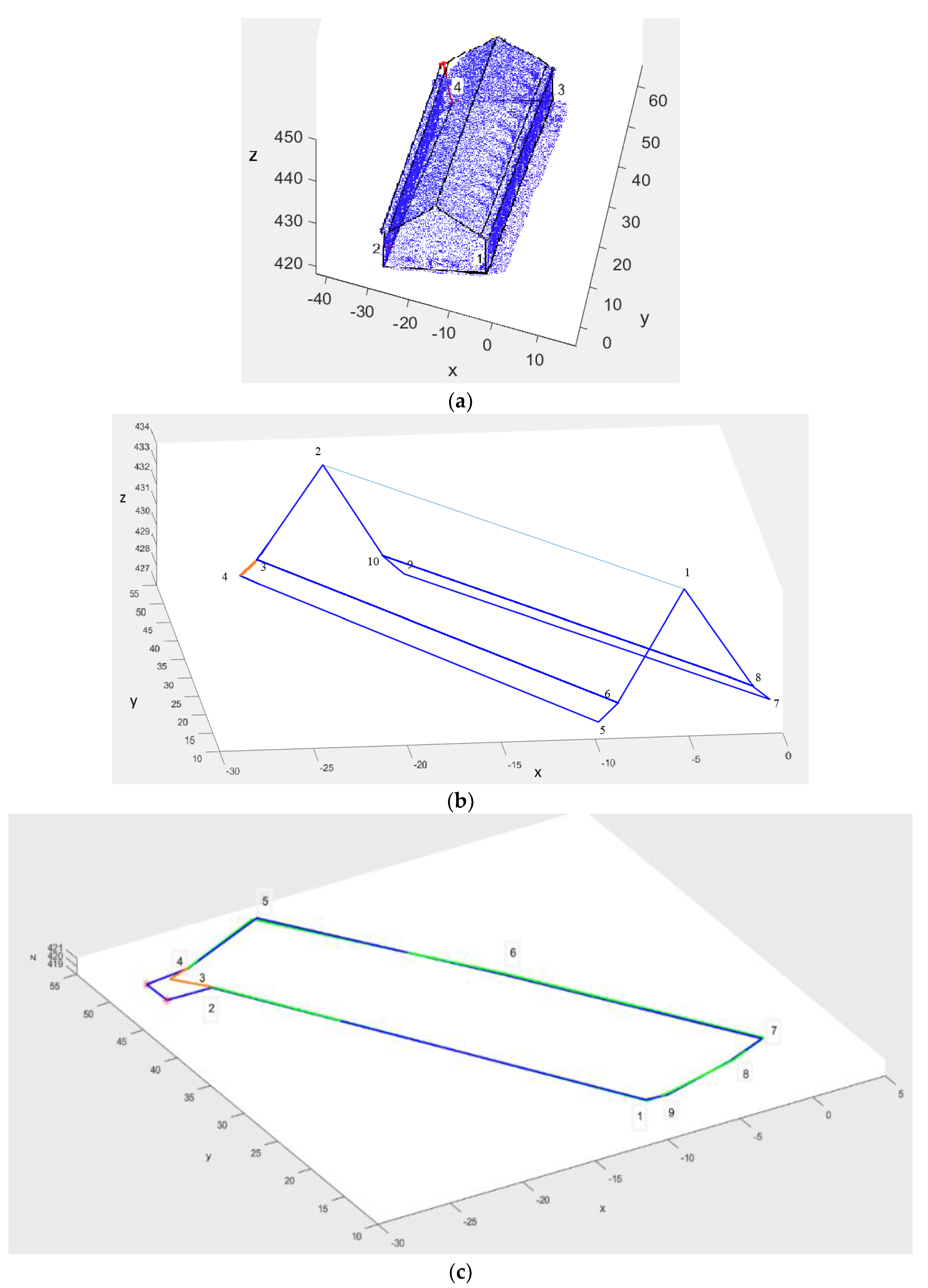
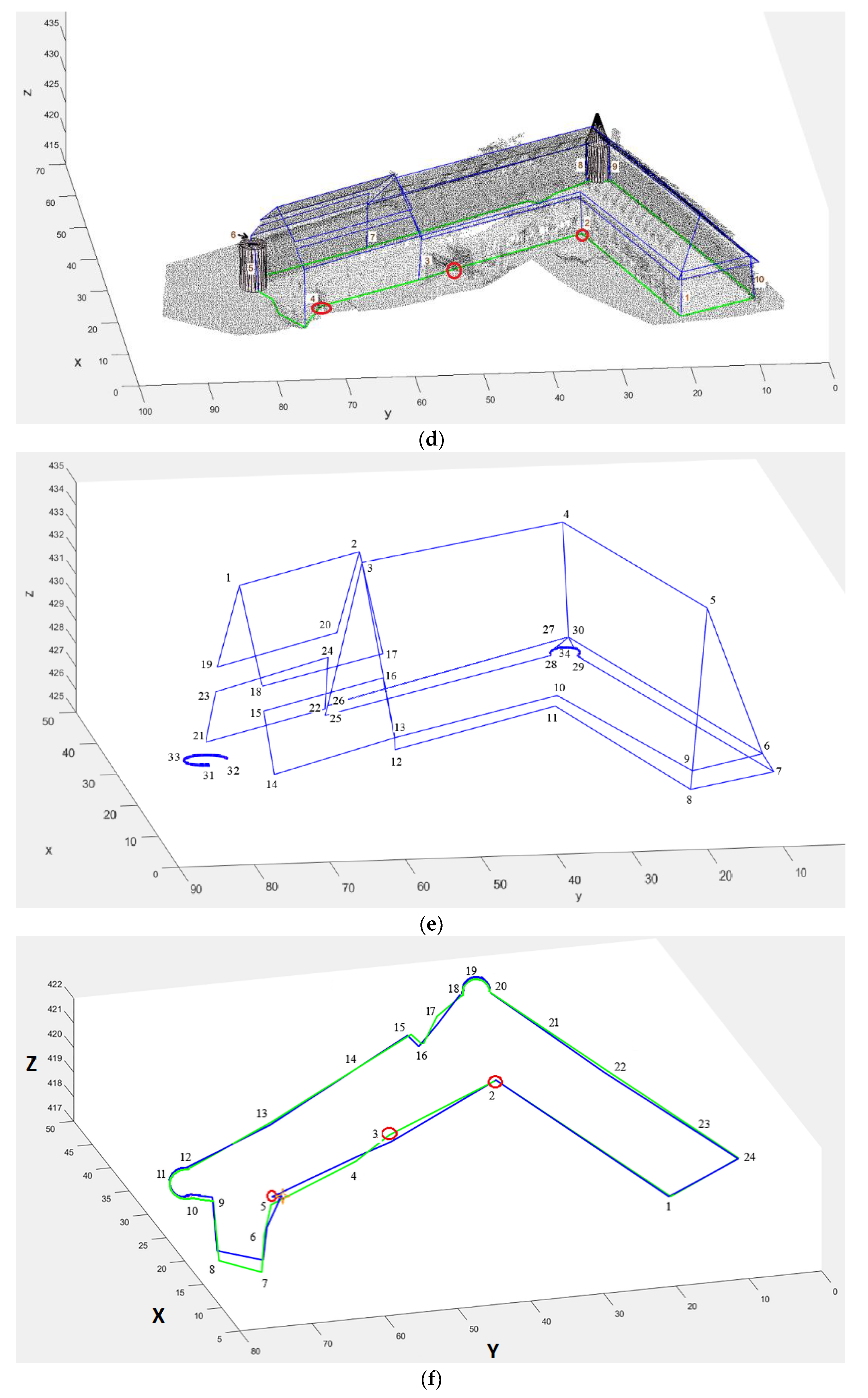
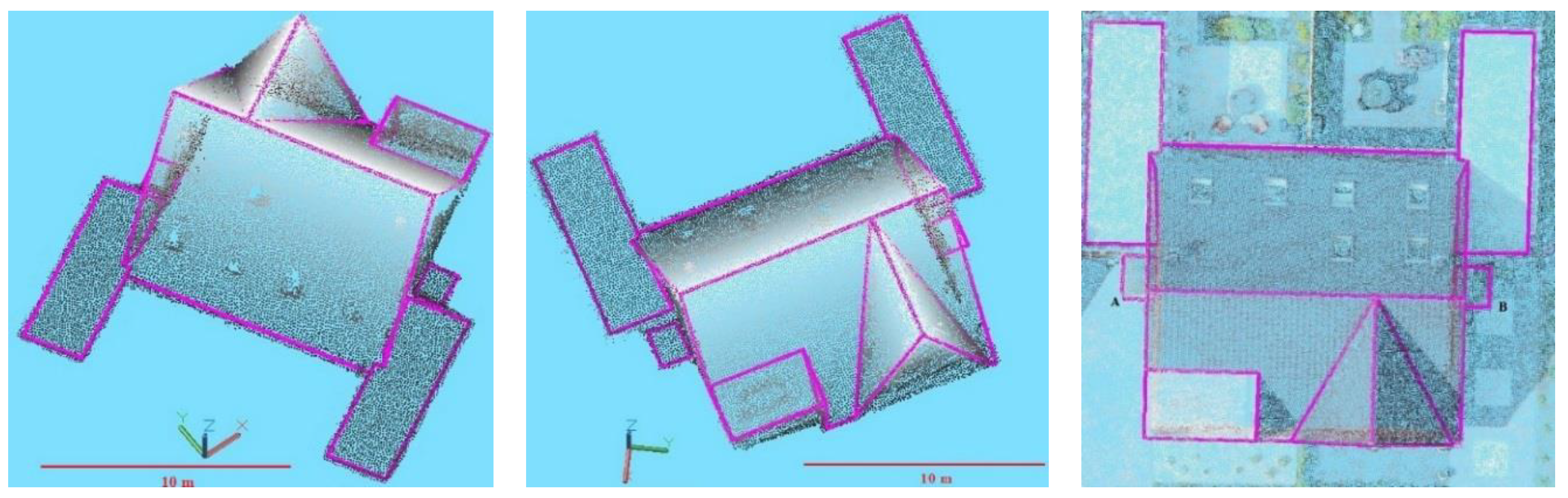
The reconstructed buildings and the extracted footprints are depicted in B-rep models of Figure 8a–f, in which red segments delineate the occluded segments of data 1 (Figure 8a–c), and red circles show the occluded vertices in data 2 (Figure 8d,f).
In order to evaluate the reconstructed models, an experienced operator digitized the reference models on the geo-referenced point clouds. In Figure 8c,f, the reconstructed footprints besides their reference data are displayed. In the reconstructed footprints, vertices with red are for building 1 (Figure 8c) and the orange star for building 2 (Figure 8f) were not generated by the reconstruction approach, though they were digitized in the reference model.
In order to evaluate geometrically the reconstructed architectural models, vertex-based criteria are used. Therefore, horizontal and vertical accuracies of the vertices are computed compared to the reference model.
In addition, in order to check the quality of the generated models, two geometric constraints, which are derived from the conceptual knowledge and were not employed in the reconstruction, are examined. The first constraint is the matter that intersecting lines of the roof includes several groups of parallel lines. The second constraint is that edges of the walls are parallel and vertical. In order to check the first constraint, angles between should-be parallel edges of the roofs and the expected parallel ridge are measured. Moreover, to check the second constraint, the zenith angle of each edge of walls is computed.
In order to assess the existence of over/under segmentation, a vertex-level evaluation of footprints is performed. In this evaluation, the vertices are counted as objects. To examine the existence of over segmentation, every triad of successive vertices of footprints are checked considering the minimum area in LoD3. So that, the middle vertex of the triad, whose area is less than the amount in the standard, is ignored. Equation (12) calculates the proposed parameter of the correctness of the vertices, which examines the existence of over segmentation.
in which ncr is the count of the correct reconstructed vertices, which have correspondences in the reference model, ncrN is the count of the correct reconstructed vertices which have no correspondences in the reference model, and nrvo is the count of the reconstructed vertices in the occluded or heavy clutter areas. According to this equation for the footprint of building 1 and for the footprint of building 2, which are less than 100%. Thus, over-segmentation happened and produced several extra segments. The reason is that we prefer to have more segments to guarantee the accuracy. The corrected footprints of buildings 1 and 2 are demonstrated in (Figure 9a,b), after removing extra vertices.
The next assessment pertains to the matter that the reference models of footprints have several vertices more than the reconstructed footprints. However, these vertices are located in the occluded areas or within heavy clutter at the feet of the buildings, which are hardly likely to be reconstructed via non-operational methods. The proposed parameter of the completeness of the vertices is defined as Equation (13) to check the existence of under segmentation.
in which ntv is the number of total vertices in the reference model, and nfvo is the count of the reference vertices in the occluded or heavy clutter areas. According to this equation, for the footprint of both buildings. Hence, no under segmentation happened and no additional vertex should be inserted in the models.
To evaluate the results of segmentation, the metrics of , proposed in [47], are computed as:
where, with regard to the reference models of buildings, (True Positive) is a detected face, which also corresponds to a building face in the reference. (False Negative) is a face from the reference models, which is not detected by our method. (False Positive) is a face, which is detected by our method but it does not exist in the reference models. The number of faces are denoted by .
These items are defined for building detection, in which buildings are mostly counted based on their outline employing different criteria. Hence a face, after projecting to the corresponding reference face, is pessimistically considered as: if it overlaps the corresponding reference face more than 70%, if it overlaps the corresponding reference face less than 70%, if the reference face does not correspond to any extracted face.
Comparing our method with other methods is not easy, because there are no datasets for benchmarking of 3D building reconstruction in this scale. Therefore, the effect of improvement in efficient RANSAC algorithm is analyzed. Thus, the aforementioned metrics are also calculated for the segmentation via the original efficient RANSAC method. The evaluation results are listed in Table 3.
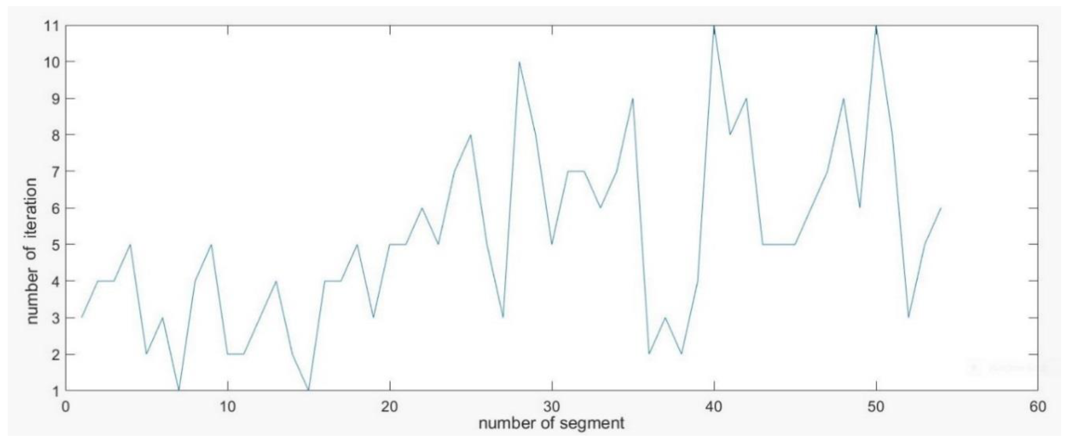
Additionally, “minimum points per primitive” computing is implemented via our method using the plane primitive in the library of the efficient RANSAC [42] and number of iterations is demonstrated in the diagram of Figure 10. This parameter is displayed for all the extracted faces of both datasets.
In the next section, outcomes of the research are analyzed and the quality control of the proposed method is discussed.
5. Discussion
To evaluate the proposed reconstruction approach, geometric accuracies of the reconstructed models are computed. Furthermore, conceptual knowledge in the form of geometrical constraints is employed. Moreover, segmentation of footprints in the viewpoint of planarity and existence of over/under segmentation is analyzed. Additionally, the overall segmentation of buildings is assessed.
According to Figure 6, the planarity criteria of the segments of the roofs are lower than and for the buildings 1 and 2, respectively. In addition, this matter is correct for the walls with the planarity better than and . Furthermore, the planarity of the segments of the grounds are better than and . These results assert the fact that the processed points lie well on the examined planes, especially on the roofs. Nonetheless, the walls carry heavy clutter due to shutters, openings, and windows.
The average accuracies of different vertices of both buildings are listed in Table 4. According to this table, the horizontal and vertical accuracies of the vertices of ridges are the highest. Average horizontal and vertical accuracies of the vertices of outer edges of eaves, generated from convex hulls, are less than of the vertices, which are calculated from the intersection. Step roofs have the average horizontal and vertical accuracies better than the eaves, on the grounds that step roofs have bigger surfaces with higher densities.
Employing the proposed plane-based method to generate footprints removes the necessity of identifying boundary points, tracing points and regularizing boundaries, which are usually indispensable steps in researches on the footprint reconstruction. The reconstructed vertices of the footprints, which are close to the big holes in the walls, suffer the lowest accuracies. Furthermore, the vertices, which are produced by the big surfaces in a flat area, have the best accuracies. Moreover, the average vertical accuracies are better than horizontal, because segments of the footprints have lower vertical variations.
Evaluation of the conceptual knowledge shows that the constraint of being parallel is observed by the edges of the roofs with errors better than . Furthermore, the edges of the walls of datasets 1 and 2 are vertical and parallel with errors less than and , respectively. Heavy clutter of shutters and big holes and intersection with the cylindrical tower and eaves result in the worst accuracies for edge 1 in data 1 and edges 8 and 9 in data 2.
According to Equations (12) and (13), the correctness of the vertices displays existence of over-segmentation for the footprints of both data. Although, the completeness demonstrates no under-segmentation because we prefer to have more segments to guarantee accuracy.
According to Table 3, the completeness, correctness, and quality criteria show better results for the proposed segmentation method compared with the original RANSAC shape detection method. Since, the original RANSAC shape detection method cannot correctly detect small segments of the eaves, especially near big dormers. Furthermore, clutter decays its detection quality, and leads to merge segments near the scaffold and builds incorrect segments. While in the proposed segmentation method, firstly the point cloud is divided and clutter decreases, then it is segmented employing the calculated sizes of the primitives. Therefore, it produces more correct segments and achieves better correctness in both datasets. In the latest section, the most significant conclusions of the research are addressed.
6. Summary and Conclusions
This paper addresses the issue of using high-density image-derived point clouds for accurate 3D rectangular building reconstruction through a novel knowledge-based approach. This approach can deal with heavy clutter and unwanted parts of UAV-based photogrammetric point clouds in order to achieve geometrical accuracy of LoD3 in 3D models of roofs, walls and footprints. A novel two-level segmentation approach is utilized based on RANSAC shape detection algorithm and contextual knowledge. At the first step, this method decreases clutter and unwanted sections and decomposes point clouds into several smaller parts employing cylinder primitives. Then, it divides each part to potential planar segments of facades, roofs or grounds. We enhance the efficient RANSAC in sizing up the segments via contextual knowledge and covariance-based analyses for both cylinder and plane primitives. The method is applied on the datasets which include building blocks with different complexity on the roofs, walls and surrounding grounds. These datasets are picked for architectural purposes. The results of the planarity criteria confirm the ability of the proposed segmentation method in grouping point clouds into planar segments, especially on the roof.
The new planar modelling method employs contextual knowledge as constraint in the least squares plane generation approach. The plane-based method of footprint generation implements points on the grounds around buildings, in a new way, along with points on neighboring walls.
The horizontal and vertical accuracies, besides the observed constraints, confirm the capability of the proposed approach in reconstructing 3D models and 3D footprints of buildings with geometrical accuracy of LoD3. For the roofs, the best accuracies are computed for the ridges and the least accuracies are calculated for the outer edges of the eaves. Moreover the vertices of the footprints achieve the best accuracies, which are in a flat area, while those close to big holes and clutter on the walls have the worst accuracies. The criteria of the correctness and completeness of the vertices are employed to reveal existence of over/under-segmentation. According to these parameters, over-segmentation happened in the footprints to guarantee accuracy, which were corrected.
The reasonable approximation of sizes of primitives is proved through better completeness, correctness and quality criteria in both datasets. The big difference of correctness criterion confirms noticeable improvement in functionality of the improved efficient RANSAC algorithm in detection of relatively small planar segments, especially near clutter areas, in complicated heterogeneous point clouds.
Low number of necessary iterations for sizes of the faces computing proves the ability of the proposed method in improving the efficient RANSAC algorithm to handle this challenging matter for planar segmentation.
Two types of knowledge are employed in this research. Contextual knowledge is used in both steps of segmentation to compute “minimum number of points per primitive” and in modelling step via defining the constraint. In addition, conceptual knowledge is utilized to calculate the outer vertices of the eaves and step roofs, in addition to establishing rules of being parallel and verticality in the evaluation step.
Finally, the geometrical evaluations besides assessments of the segmentation confirm that the proposed approach can successfully employ high-density photogrammetric point clouds generated from UAV imagery as the only source of data in 3D reconstruction of buildings and their footprints with the geometrical accuracy of LoD3. In our ongoing work, we would like to exploit color information of photogrammetric point cloud to enrich the 3D reconstructed models of buildings semantically.
Author Contributions
All the authors contributed to the concept of the research. S.M. performed the implementation of the algorithm, analysis and evaluation of the results and wrote the article. M.H. carried out the data acquisition and pre-processing and reviewed the manuscript. M.J.V.Z. supervised the research, conducted the discussions moreover, reviewed and improved the manuscript.
Acknowledgments
This study was partly supported by Deutscher Akademischer AustauschDienst for Shirin Malihi. The authors are thankful of H. Arefi from the School of Surveying and Geospatial Engineering, University of Tehran for useful insightful suggestions. The authors appreciate valuable comments and advice of M. Gerke from the Institute of Geodesy and Photogrammetry, Technische Universität Braunschweig. We acknowledge support by the German Research Foundation (DFG) and the Open Access Publication Funds of the Technische Universität Braunschweig.
Conflicts of Interest
The authors declare no conflicts of interest.
Appendix A

Table A1.
Calibration report of the Sony camera of ILCE-7R.
| Properties | Data |
|---|---|
| Focal length | 35 mm |
| Resolution | 7360 × 4912 |
| Pixel size | 4.89 × 4.89 µm |
| Fx | 7429.05 pixel |
| Fy | 7429.05 pixel |
| k1 | 0.0557213 |
| k2 | −0.219064 |
| k3 | −0.0120905 |
| k4 | 0 |
| skew | 0 |
| cx | 3650.54 |
| cy | 2463.08 |
| P1 | −0.000600474 |
| P2 | 0.000548429 |
Appendix B
Figure A1.
Approximation of the step roof’s number of points. (a,b) Recognizing the edges of the roof as the borders of half-planes via histogram of , and (c) generation of the main edges of the roof. (Units of axes in (b,c) are m).
Figure A1.
Approximation of the step roof’s number of points. (a,b) Recognizing the edges of the roof as the borders of half-planes via histogram of , and (c) generation of the main edges of the roof. (Units of axes in (b,c) are m).


Appendix C
The optical data from a small building is captured using an Olympus camera with the calibrated focal length of 16.53 mm and average GSD of 1.7 cm. These images are utilized to produce the image-derived point cloud with the average linear density of 15 point/m (Figure A2). These data do not bear oblique imaging. Therefore, points on walls gain a low density. In order to reconstruct a roof with different intersections and step roofs, points on the roof are segregated by height thresholding (Figure A2).
Figure A2.
Point cloud of the building and roof (m).

These data contain low clutter and heterogeneity. Therefore, points enter directly into second step of the improved efficient RANSAC algorithm employing the parameters in Table A2.
Table A2.
Parameters of the efficient RANSAC for planar shape detection.
| Parameter | Values |
|---|---|
| Maximum distance to the primitive (m) | 0.01–0.10 |
| Maximum normal deviation (degree) | 1–5 |
| Sampling resolution (m) | 0.1 |
| Overlooking probability (%) | 95 |
| Minimum points per primitive |
is computed via Equation (8). The histogram of cosine of the inclination angle of is demonstrated in Figure A3. Two intersected vertical edges at the lowest height are set as axes. Investigation of step roofs leads in coefficients of and in directions of at height of (Figure A4), so that Equation (A1) works out. It means in three different heights, the parallel planes appear which are horizontal and their points occupy bins around 0 in Figure A3. Hence, these bins (bin0) are employed to segment horizontal step roofs.
Areas of the horizontal segments are approximated employing horizontal edges in Figure A4 through Equation (A2), where at height of is horizontal edge in x-z view, is horizontal edge in y-z view and is the area of the plane, which is surrounded by and . Number of points of the horizontal step roof in height of () is estimated via Equation (A3).
Figure A3.
The histogram of cosine of the inclination angle of .

Figure A4.
The point cloud from (a) x–z view and (b) y–z view (m).

Figure A5 shows the reconstructed planar models of the point cloud. The vertices which are placed on at least three planes are computed through the method of Section 2.2 and other vertices are generated via the regularized convex hulls, within possible constraint of intersection with other planar models.
Figure A5.
Reconstructed planar models (m).

The reconstructed B-rep model of the roof is displayed in Figure A6. Vertex-based relative geometrical accuracy of the model is achieved by comparison with the ground truth model, which is generated via digitization on the point cloud. The consequent relative horizontal and vertical accuracies are (0.20, 0.29) m respectively. Consequently, the proposed method can reconstruct the roof with different intersections of planar patches and various horizontal step roofs in different heights.
Figure A6.
Reconstructed B-rep model of the roof is superimposed on the point cloud (m).

References
- Haala, N.; Kada, M. An update on automatic 3D building reconstruction. J. Photogramm. Remote Sens. 2010, 65, 570–580. [Google Scholar] [CrossRef]
- Gröger, G.; Kolbe, T.H.; Nagel, C.; Häfele, K.-H. OGC City Geography Markup Language (CityGML) Encoding Standard. 2012. Available online: https://portal.opengeospatial.org/files/?artifact_id=47842 (accessed on 1 January 2018).
- Donkers, S. Automatic Generation of CityGML LoD3 Building Models from IFC Models. Master’s Thesis, TU Delft, Delft, The Netherlands, 2013. [Google Scholar]
- Löwner, M.; Benner, J.; Gröger, G.; Häfele, K. New Concepts for Structuring 3D City Models—An Extended Level of Detail Concept for CityGML Buildings. In Computational Science and Its Applications—ICCSA 2013; Lecture Notes in Computer Science; Springer: Berlin/Heidelberg, Germany, 2013; Volume 7973. [Google Scholar]
- Tarsha-Kurdi, F.; Landes, T.; Grussenmeyer, P.; Koehl, M. Model-driven and data-driven approaches using LIDAR data: Analysis and comparison. Int. Arch. Photogramm. Remote Sens. 2007, 36, 87–92. [Google Scholar]
- Elberink, S.O.; Vosselman, G. Building reconstruction by target based graph matching on incomplete laser data: Analysis and limitations. Sensors 2009, 9, 6101–6118. [Google Scholar] [CrossRef] [PubMed]
- Wichmann, A.; Jung, J.; Sohn, G.; Kada, M.; Ehlers, M. Integration of building knowledge into binary space partitioning for the reconstruction of regularized building models. ISPRS Ann. Photogramm. Remote Sens. Spat. Inf. Sci. 2015, II-3/W5, 541–548. [Google Scholar] [CrossRef]
- Satari, M.; Samadzadegan, F.; Azizi, A.; Maas, H.-G. A multi-resolution hybrid approach for building model reconstruction from LIDAR data. Photogramm. Rec. 2012, 27, 330–359. [Google Scholar] [CrossRef]
- Zolanvari, S.M.I.; Laefer, D.F.; Natanzi, A.S. Three-dimensional building façade segmentation and opening area detection from point clouds. ISPRS J. Photogramm. Remote Sens. 2018. [Google Scholar] [CrossRef]
- Pahlavani, P.; Amini Amirkolaee, H.; Bigdeli, B. 3D reconstruction of buildings from LiDAR data considering various types of roof structures. Int. J. Remote Sens. 2017, 38, 1451–1482. [Google Scholar] [CrossRef]
- Jung, J.; Jwa, Y.; Sohn, G. Implicit regularization for reconstructing 3D building rooftop models using airborne LiDAR data. Sensors 2017, 17, 621. [Google Scholar] [CrossRef] [PubMed]
- Huang, H.; Brenner, C.; Sester, M. A generative statistical approach to automatic 3D building roof reconstruction from laser scanning data. ISPRS J. Photogramm. Remote Sens. 2013, 79, 29–43. [Google Scholar] [CrossRef]
- Wang, F.; Xi, X.; Wang, C.; Xiao, Y.; Wan, Y. Boundary regularization and building reconstruction based on terrestrial laser scanning data. In Proceedings of the 2013 IEEE International Geoscience and Remote Sensing Symposium—IGARSS, Melbourne, Australia, 21–26 July 2013; pp. 1509–1512. [Google Scholar]
- Hammoudi, K. Contributions to the 3D City Modeling: 3D Polyhedral Building Model Reconstruction from Aerial Images and 3D Facade Modeling from Terrestrial 3D Point Cloud and Images; Université Paris-Est: Champs-sur-Marne, France, 2011. [Google Scholar]
- Rupnik, E.; Pierrot-Deseilligny, M.; Delorme, A. 3D reconstruction from multi-view VHR-satellite images in MicMac. ISPRS J. Photogramm. Remote Sens. 2018, 139, 201–211. [Google Scholar] [CrossRef]
- Haala, N.; Rothermel, M.; Cavegn, S. Extracting 3D urban models from oblique aerial images. In Proceedings of the 2015 Joint Urban Remote Sensing Event (JURSE), IEEE, Lausanne, Switzerland, 30 March–1 April 2015; pp. 1–4. [Google Scholar]
- Xiao, J.; Gerke, M.; Vosselman, G. Building extraction from oblique airborne imagery based on robust façade detection. ISPRS J. Photogramm. Remote Sens. 2012, 68, 56–68. [Google Scholar] [CrossRef]
- Dahlke, D.; Linkiewicz, M.; Meissner, H. True 3D building reconstruction: Façade, roof and overhang modelling from oblique and vertical aerial imagery. Int. J. Image Data Fusion 2015, 6, 314–329. [Google Scholar] [CrossRef]
- Vetrivel, A.; Gerke, M.; Kerle, N.; Vosselman, G. Segmentation of UAV-based images incorporating 3D point cloud information. In Proceedings of the Photogrammetric Image Analysis, PIA15 + High-Resolution Earth Imaging for Geospatial Information, HRIGI15: Joint ISPRS Conference, Munich, Germany, 25–27 March 2015; Volume XL-3/W2, pp. 261–268. [Google Scholar]
- Xu, Z.; Wu, L.; Zhang, Z. Use of active learning for earthquake damage mapping from UAV photogrammetric point clouds. Int. J. Remote Sens. 2017, 8, 1–28. [Google Scholar] [CrossRef]
- Henn, A.; Gröger, G.; Stroh, V.; Plümer, L. Model driven reconstruction of roofs from sparse LIDAR point clouds. ISPRS J. Photogramm. Remote Sens. 2013, 76, 17–29. [Google Scholar] [CrossRef]
- Fu, K.; Zhang, Y.; Sun, X.; Diao, W.; Wu, B.; Wang, H. Automatic building reconstruction from high resolution InSAR data using stochastic geometrical model. In Proceedings of the 2016 IEEE International Geoscience and Remote Sensing Symposium (IGARSS), Beijing, China, 10–15 July 2016; pp. 1579–1582. [Google Scholar]
- Salehi, A.; Mohammadzadeh, A. Building Roof Reconstruction Based on Residue Anomaly Analysis and Shape Descriptors from Lidar and Optical Data. Photogramm. Eng. Remote Sens. 2017, 83, 281–291. [Google Scholar] [CrossRef]
- Yang, L.; Sheng, Y.; Wang, B. 3D reconstruction of building facade with fused data of terrestrial LiDAR data and optical image. Opt. Int. J. Light Electron Opt. 2016, 127, 2165–2168. [Google Scholar] [CrossRef]
- Pu, S.; Vosselman, G. Building facade reconstruction by fusing terrestrial laser points and images. Sensors 2009, 9, 4525–4542. [Google Scholar] [CrossRef] [PubMed]
- Ameri, B.; Fritsch, D. Automatic 3D building reconstruction using plane-roof structures. In Proceedings of the American Society for Photogrammetry and Remote Sensing, Washington, DC, USA, 22–26 May 2000. [Google Scholar]
- Malihi, S.; Valadan Zoej, M.J.; Hahn, M.; Mokhtarzade, M.; Arefi, H. 3D building reconstruction using dense photogrammetric point cloud. ISPRS Int. Arch. Photogramm. Remote Sens. Spat. Inf. Sci. 2016, XLI-B3, 71–74. [Google Scholar] [CrossRef]
- Haala, N.; Cavegn, S. High density aerial image matching: State-of-the-art and future prospects. ISPRS Int. Arch. Photogramm. Remote Sens. Spat. Inf. Sci. 2016, XLI-B4, 625–630. [Google Scholar] [CrossRef]
- Ressl, C.; Brockmann, H.; Mandlburger, G.; Pfeifer, N. Dense Image Matching vs. Airborne Laser Scanning—Comparison of two methods for deriving terrain models. Photogramm. Fernerkund. Geoinf. 2016, 2016, 57–73. [Google Scholar] [CrossRef]
- Cavegn, S.; Haala, N.; Nebiker, S.; Rothermel, M.; Tutzauer, P. Benchmarking high density image matching for oblique airborne imagery. ISPRS Int. Arch. Photogramm. Remote Sens. Spat. Inf. Sci. 2014, XL-3, 45–52. [Google Scholar] [CrossRef]
- Xiong, B.; Oude Elberink, S.; Vosselman, G. Building modeling from noisy photogrammetric point clouds. ISPRS Ann. Photogramm. Remote Sens. Spat. Inf. Sci. 2014, II-3, 197–204. [Google Scholar] [CrossRef]
- Tutzauer, P.; Haala, N. Façade reconstruction using geometric and radiometric point cloud information. ISPRS Int. Arch. Photogramm. Remote Sens. Spat. Inf. Sci. 2015, XL-3/W2, 247–252. [Google Scholar] [CrossRef]
- Nex, F.; Remondino, F. UAV for 3D mapping applications: A review. Appl. Geomat. 2014, 6, 1–15. [Google Scholar] [CrossRef]
- Colomina, I.; Molina, P. Unmanned aerial systems for photogrammetry and remote sensing: A review. ISPRS J. Photogramm. Remote Sens. 2014, 92, 79–97. [Google Scholar] [CrossRef]
- Kolbe, T.H.; Gröger, G.; Plümer, L. CityGML: Interoperable access to 3D city models. In Geo-information for Disaster Management; Springer: Berlin/Heidelberg, Germany, 2005; pp. 883–899. [Google Scholar]
- Awrangjeb, M. Using point cloud data to identify, trace, and regularize the outlines of buildings. Int. J. Remote Sens. 2016, 37, 551–579. [Google Scholar] [CrossRef] [Green Version]
- Dai, Y.; Gong, J.; Li, Y.; Feng, Q. Building segmentation and outline extraction from UAV image-derived point clouds by a line growing algorithm. Int. J. Digit. Earth 2017, 10, 1077–1097. [Google Scholar] [CrossRef]
- Dorninger, P.; Pfeifer, N. A comprehensive automated 3D approach for building extraction, reconstruction, and regularization from airborne laser scanning point clouds. Sensors 2008, 8, 7323–7343. [Google Scholar] [CrossRef] [PubMed]
- He, Y.; Zhang, C.; Awrangjeb, M.; Fraser, C.S. Automated reconstruction of walls from airborne lidar data for complete 3D building modelling. In Proceedings of the International Archives of the Photogrammetry, Remote Sensing and Spatial Information Sciences, Melbourne, Australia, 25 August–1 September 2012; pp. 115–120. [Google Scholar]
- Pu, S.; Vosselman, G. Knowledge based reconstruction of building models from terrestrial laser scanning data. ISPRS J. Photogramm. Remote Sens. 2009, 64, 575–584. [Google Scholar] [CrossRef]
- Nguyen, A.; Le, B. 3D point cloud segmentation: A survey. In Proceedings of the 6th Conference on Robotics, Automation and Mechatronics (RAM), Manila, Philippines, 12–15 November 2013; pp. 225–230. [Google Scholar]
- Schnabel, R.; Wahl, R.; Klein, R. Efficient RANSAC for point-cloud shape detection. Comput. Graph. Forum 2007, 26, 214–226. [Google Scholar] [CrossRef]
- Online Statistics Education: A Free Resource for Introductory Statistics. Available online: http://onlinestatbook.com/mobile/index.html (accessed on 11 May 2018).
- Rusu, R.B. PCL Tutorial. Available online: http://pointclouds.org/documentation/tutorials/statistical_outlier.php (accessed on 12 August 2016).
- Gross, H.; Thoennessen, U. Extraction of lines from laser point clouds. In Proceedings of the Symposium of ISPRS Commission III Photogrammetric Computer Vision, Bonn, Germany, 20–22 September 2006; Volume 36, pp. 86–91. [Google Scholar]
- Sampath, A.; Shan, J. Segmentation and Reconstruction of Polyhedral Building Roofs From Aerial Lidar Point Clouds. IEEE Trans. Geosci. Remote Sens. 2010, 48, 1554–1567. [Google Scholar] [CrossRef]
- Rutzinger, M.; Rottensteiner, F.; Pfeifer, N. A Comparison of Evaluation Techniques for Building Extraction From Airborne Laser Scanning. IEEE J. Sel. Top. Appl. Earth Obs. Remote Sens. 2009, 2, 11–20. [Google Scholar] [CrossRef]
Figure 1.
The general diagram of the proposed 3D reconstruction method.

Figure 2.
Two building blocks and their surrounding areas.

Figure 3.
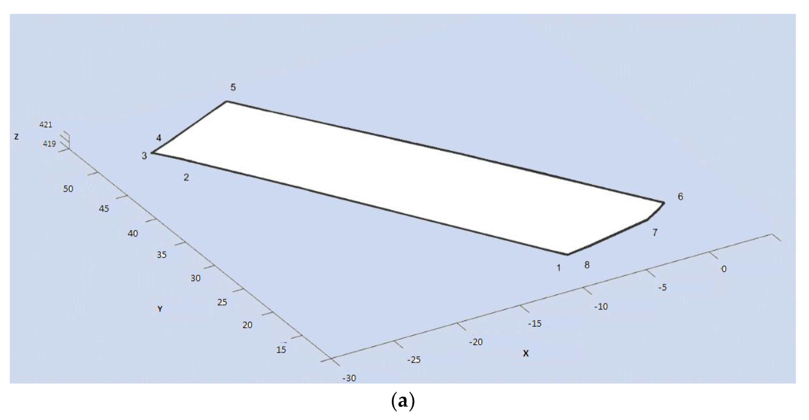
The first level of segmentation: (a,c) using cylinder primitive in dividing point clouds of the buildings, to (d,f) several parts; (b) using cylinder primitive to (e) segment point cloud of the footprint. (Units of axes are m).
Figure 3.
The first level of segmentation: (a,c) using cylinder primitive in dividing point clouds of the buildings, to (d,f) several parts; (b) using cylinder primitive to (e) segment point cloud of the footprint. (Units of axes are m).

Figure 4.
Approximation of µ. (a) The eigenvectors of an ellipse and a circle-shaped neighborhood around the centre point. (b) The histogram of .
Figure 4.
Approximation of µ. (a) The eigenvectors of an ellipse and a circle-shaped neighborhood around the centre point. (b) The histogram of .

Figure 5.
Approximating number of points of the planar segments for the efficient RANSAC. (a) The histogram of cosine of the inclination angle of . (b–e) Histograms of the inclination angle (in radian) of the footprint, roof, step roof and walls. (b’,c’,d’,e’) corresponding marked points in clusters (units of axes are m).


Figure 6.
Planarity. (a,c) for the point clouds of the roof (5–8, 7–19), the walls (1–4, 1–7), and (b,d) for the point clouds of the grounds. (a,b) point clouds of building 1, and (c,d) point clouds of building 2.
Figure 6.
Planarity. (a,c) for the point clouds of the roof (5–8, 7–19), the walls (1–4, 1–7), and (b,d) for the point clouds of the grounds. (a,b) point clouds of building 1, and (c,d) point clouds of building 2.

Figure 7.
Superimposing the constructed models on point clouds of (a) building 1 and (b) building 2. (Units of axes are m).
Figure 7.
Superimposing the constructed models on point clouds of (a) building 1 and (b) building 2. (Units of axes are m).

Figure 8.
The reconstructed B-rep models. (a,d) superimposing the reconstructed buildings on the point clouds, (b,e) the reconstructed roofs, (c,f) the reconstructed footprints (green) besides the reference data (blue). (Units of axes are m).
Figure 8.
The reconstructed B-rep models. (a,d) superimposing the reconstructed buildings on the point clouds, (b,e) the reconstructed roofs, (c,f) the reconstructed footprints (green) besides the reference data (blue). (Units of axes are m).


Figure 9.
The corrected footprint, (a) of building 1 and (b) of building 2. (Units of axes are m).


Figure 10.
Number of iterations for “minimum points per primitive” computing for planes.

Table 1.
Parameters of the efficient RANSAC algorithm for cylindrical shape detection.
| Parameter | Value (s) |
|---|---|
| Maximum distance to the primitive (m) | 0.15 |
| Maximum normal deviation (degree) | 10–15 |
| Sampling resolution (m) | 0.1 |
| Overlooking probability (%) | 85–90 |
| Minimum points per primitive | Equation (5) |
Table 2.
Parameters of the efficient RANSAC for planar shape detection.
| Parameter | Values |
|---|---|
| Maximum distance to the primitive (m) | 0.01–0.05 |
| Maximum normal deviation (degree) | 1–8 |
| Sampling resolution (m) | 0.03–0.1 |
| Overlooking probability (%) | 95–99 |
| Minimum points per primitive |
Table 3.
Performance evaluation of the proposed segmentation method compared with the original RANSAC shape detection method.
Table 3.
Performance evaluation of the proposed segmentation method compared with the original RANSAC shape detection method.
| Building1 | Building2 | Building1 | Building2 | Building1 | Building2 | |
|---|---|---|---|---|---|---|
| the original efficient RANSAC method | 88% | 86% | 88% | 83% | 78% | 73% |
| Our method | 90% | 88% | 100% | 97% | 90% | 86% |
Table 4.
The average accuracies of the reconstructed vertices of roofs and footprints.
| Building 1 Accuracy (m) | Building 2 Accuracy (m) | ||||
|---|---|---|---|---|---|
| Horizontal | Vertical | Horizontal | Vertical | ||
| Roof | Vertices of ridges | 0.11 | 0.11 | 0.09 | 0.10 |
| Vertices of outer edges of eaves | 0.24 | 0.23 | 0.35 | 0.37 | |
| Vertices of step roofs | - | - | 0.28 | 0.32 | |
| Vertices calculated from intersection | 0.14 | 0.21 | 0.21 | 0.23 | |
| Vertices of cylinders | - | - | 0.29 | 0.30 | |
| Vertices of footprints | 0.19 | 0.17 | 0.28 | 0.24 | |
© 2018 by the authors. Licensee MDPI, Basel, Switzerland. This article is an open access article distributed under the terms and conditions of the Creative Commons Attribution (CC BY) license (http://creativecommons.org/licenses/by/4.0/).
Share and Cite
MDPI and ACS Style
Malihi, S.; Valadan Zoej, M.J.; Hahn, M. Large-Scale Accurate Reconstruction of Buildings Employing Point Clouds Generated from UAV Imagery. Remote Sens. 2018, 10, 1148. https://0-doi-org.brum.beds.ac.uk/10.3390/rs10071148
AMA Style
Malihi S, Valadan Zoej MJ, Hahn M. Large-Scale Accurate Reconstruction of Buildings Employing Point Clouds Generated from UAV Imagery. Remote Sensing. 2018; 10(7):1148. https://0-doi-org.brum.beds.ac.uk/10.3390/rs10071148
Chicago/Turabian StyleMalihi, Shirin, Mohammad Javad Valadan Zoej, and Michael Hahn. 2018. "Large-Scale Accurate Reconstruction of Buildings Employing Point Clouds Generated from UAV Imagery" Remote Sensing 10, no. 7: 1148. https://0-doi-org.brum.beds.ac.uk/10.3390/rs10071148
Note that from the first issue of 2016, this journal uses article numbers instead of page numbers. See further details here.