TerraSAR-X Time Series Fill a Gap in Spaceborne Snowmelt Monitoring of Small Arctic Catchments—A Case Study on Qikiqtaruk (Herschel Island), Canada

 ,
,  ,
,
Abstract
:
1. Introduction
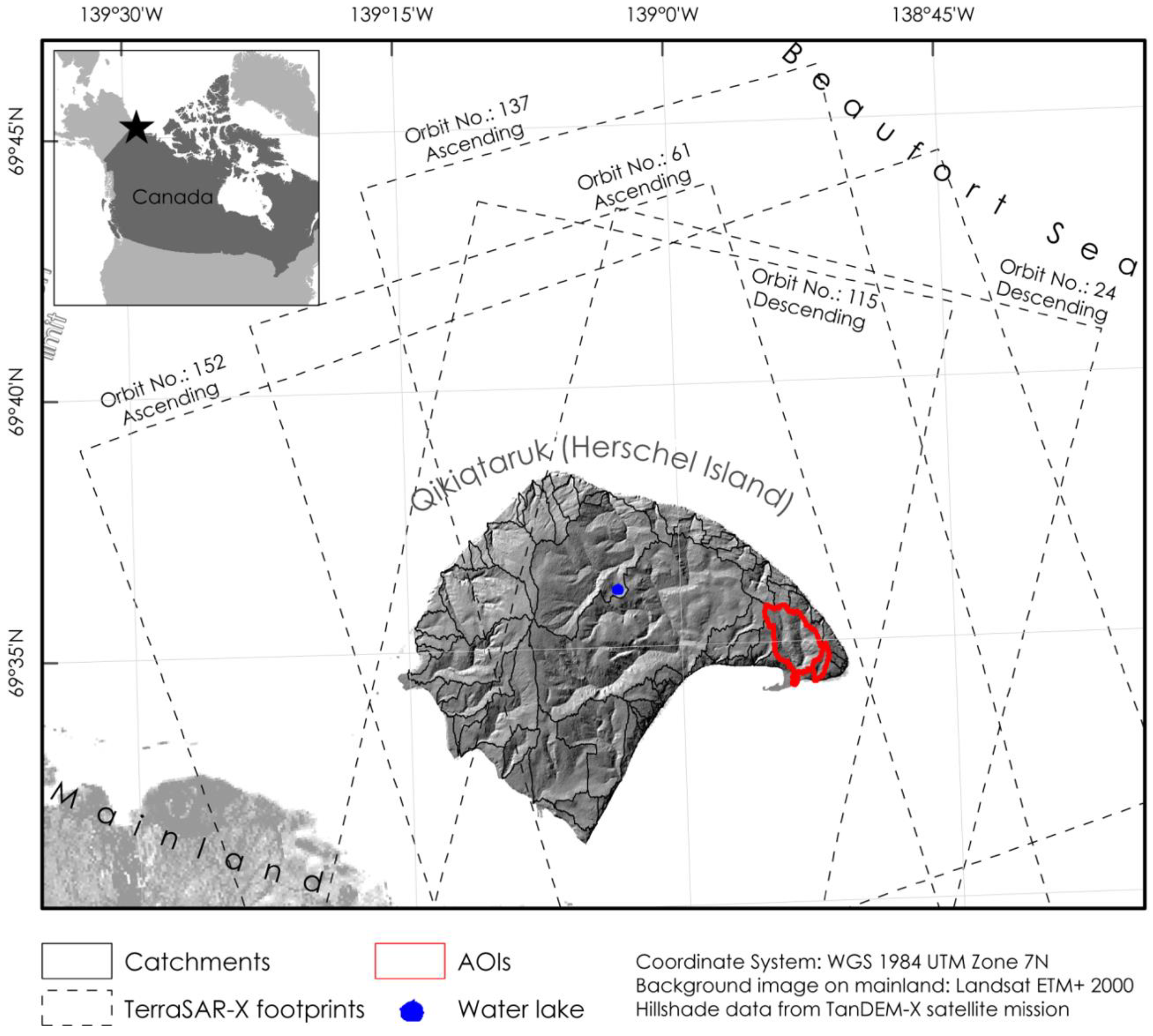
2. Study Area
3. Data & Methods
3.1. SAR Satellite Data
3.2. Optical Satellite Data
3.3. In situ Time-Lapse Camera Data
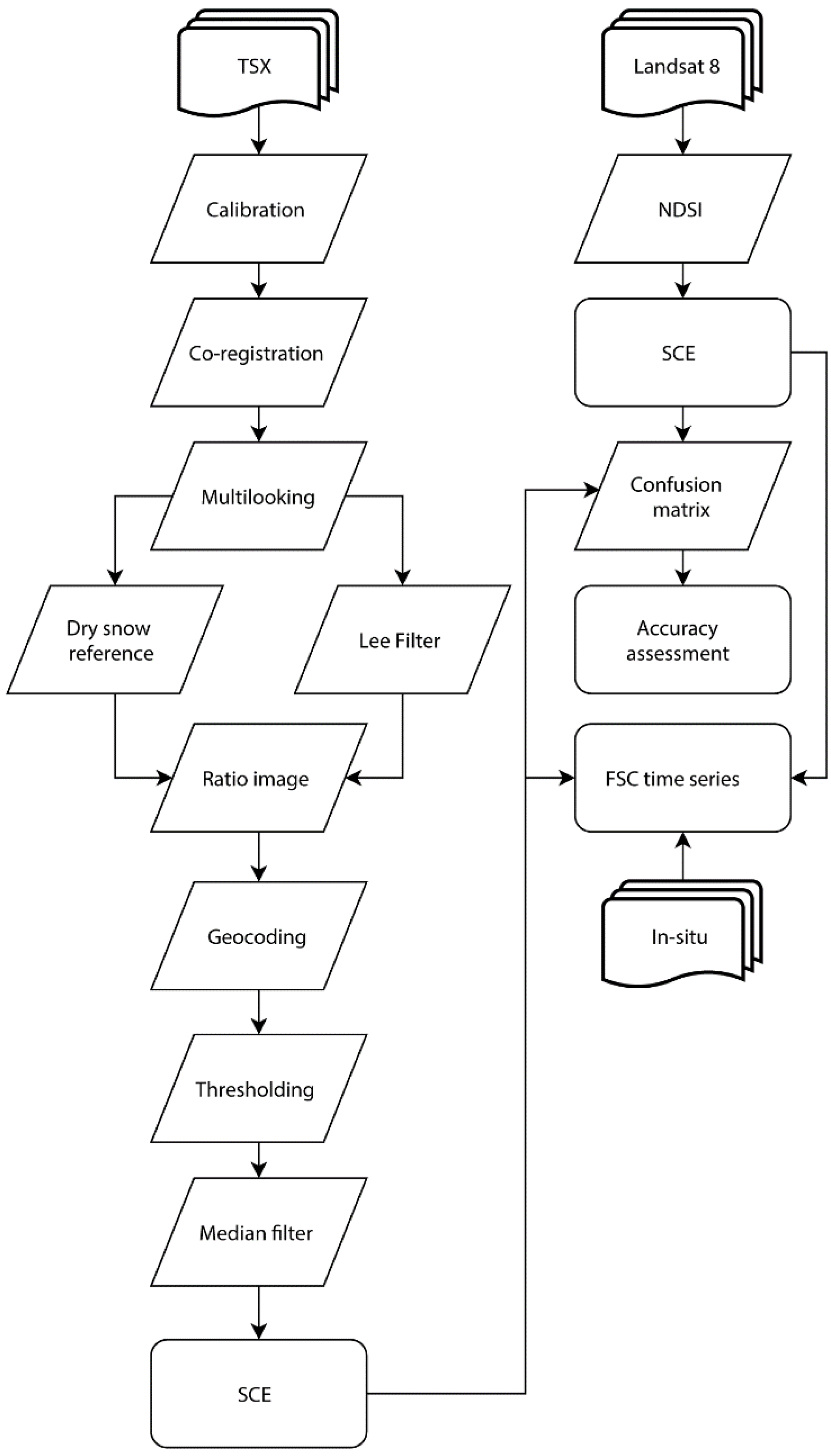
3.4. Snow Cover Extent from TerraSAR-X
3.5. Snow Cover Extent from Landsat 8
3.6. Accuracy Assessment of TerraSAR-X Snow Cover Extent
3.7. Fractional Snow Cover Time Series Analysis
4. Results
4.1. Evaluation of Backscatter Time Series
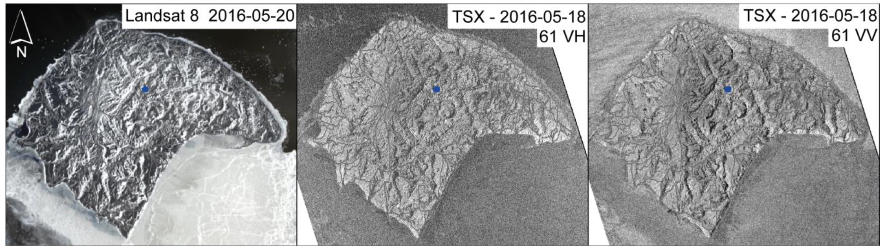
4.2. Evaluation of TSX Snow Cover Extent
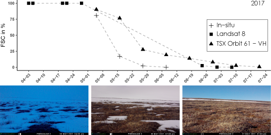
4.3. Time Series of Fractional Snow Cover in All Catchments
4.4. Time Series of Fractional Snow Cover in Three Small Catchments
5. Discussion
5.1. Spatiotemporal Monitoring of Snowmelt Dynamics Using TSX
5.2. Technical Considerations for Using TSX for Wet Snow Detection
6. Conclusions
Supplementary Materials
Author Contributions
Funding
Acknowledgments
Conflicts of Interest
References
- Ling, F.; Zhang, T. Impact of the timing and duration of seasonal snow cover on the active layer and permafrost in the Alaskan Arctic. Permafr. Periglac. Process. 2003, 14, 141–150. [Google Scholar] [CrossRef]
- Zhang, T.; Stamnes, K. Impact of climatic factors on the active layer and permafrost at Barrow, Alaska. Permafr. Periglac. Process. 1998, 9, 229–246. [Google Scholar] [CrossRef]
- Zhang, T.; Osterkamp, T.E.; Stamnes, K. Influence of the depth hoar layer of the seasonal snow cover on the ground thermal regime. Water Resour. Res. 1996, 32, 2075–2086. [Google Scholar] [CrossRef]
- Johansson, M.; Callaghan, T.V.; Bosiö, J.; Åkerman, H.J.; Jackowicz-Korczynski, M.; Christensen, T.R. Rapid responses of permafrost and vegetation to experimentally increased snow cover in sub-arctic Sweden. Environ. Res. Lett. 2013, 8, 035025. [Google Scholar] [CrossRef] [Green Version]
- Semenchuk, P.R.; Elberling, B.; Amtorp, C.; Winkler, J.; Rumpf, S.; Michelsen, A.; Cooper, E.J. Deeper snow alters soil nutrient availability and leaf nutrient status in high Arctic tundra. Biogeochemistry 2015, 124, 81–94. [Google Scholar] [CrossRef] [Green Version]
- Schimel, J.P.; Bilbrough, C.; Welker, J.A.; Schimel, J.P.; Bilbrough, C.; Welker, J.M. Increased snow depth affects microbial activity and nitrogen mineralization in two Arctic tundra communities. Soil Biol. Biochem. 2004, 36, 217–227. [Google Scholar] [CrossRef] [Green Version]
- Krab, E.J.; Roennefarth, J.; Becher, M.; Blume-Werry, G.; Keuper, F.; Klaminder, J.; Kreyling, J.; Makoto, K.; Milbau, A.; Dorrepaal, E. Winter warming effects on tundra shrub performance are species-specific and dependent on spring conditions. J. Ecol. 2018, 106, 599–612. [Google Scholar] [CrossRef]
- Ballantyne, C.K. The Hydrologic Significance of Nivation Features in Permafrost Areas. Geogr. Ann. Ser. A Phys. Geogr. 1978, 60, 51–54. [Google Scholar] [CrossRef]
- Schimel, J.P.; Kielland, K.; Chapin, F.S. Nutrient Availability and Uptake by Tundra Plants. In Landscape Function and Disturbance in Arctic Tundra; Springer: Berlin/Heidelberg, Germany, 1996; pp. 203–221. [Google Scholar]
- Ostendorf, B.; Quinn, P.; Beven, K.; Tenhunen, J.D. Hydrological Controls on Ecosystem Gas Exchange in an Arctic Landscape. In Landscape Function and Disturbance in Arctic Tundra; Springer: Berlin/Heidelberg, Germany, 1996; pp. 369–386. [Google Scholar]
- Hobbie, S.E.; Chapin, F.S. Winter regulation of tundra litter carbon and nitrogen dynamics. Biogeochemistry 1996, 35, 327–338. [Google Scholar] [CrossRef]
- Bartsch, A.; Kidd, R.A.; Wagner, W.; Bartalis, Z. Temporal and spatial variability of the beginning and end of daily spring freeze/thaw cycles derived from scatterometer data. Remote Sens. Environ. 2007, 106, 360–374. [Google Scholar] [CrossRef]
- Brooks, P.D.; Grogan, P.; Templer, P.H.; Groffman, P.; Öquist, M.G.; Schimel, J. Carbon and Nitrogen Cycling in Snow-Covered Environments. Geogr. Compass 2011, 5, 682–699. [Google Scholar] [CrossRef]
- Woo, M. Hydrology of a small Canadian High Arctic basin during the snowmelt period. Catena 1976, 3, 155–168. [Google Scholar] [CrossRef]
- Billings, W.D.; Mooney, H.A. The Ecology of Arctic Plants. Biol. Rev. 1968, 43, 481–529. [Google Scholar] [CrossRef]
- Hinzman, L.D.; Kane, D.L.; Benson, C.S.; Everett, K.R. Energy Balance and Hydrological Processes in an Arctic Watershed. In Landscape Function and Disturbance in Arctic Tundra; Springer: Berlin/Heidelberg, Germany, 1996; pp. 131–154. [Google Scholar]
- Pohl, S.; Marsh, P. Modelling the spatial-temporary variability of spring snowmelt in an arctic catchment. Hydrol. Process. 2006, 20, 1773–1792. [Google Scholar] [CrossRef]
- Billings, W.D.; Bliss, L.C. An alpine snowbank environment and its effects on vegetation, plant development, and productivity. Ecology 1959, 40, 388–397. [Google Scholar] [CrossRef]
- Bjorkman, A.D.; Elmendorf, S.C.; Beamish, A.L.; Vellend, M.; Henry, G.H.R. Contrasting effects of warming and increased snowfall on Arctic tundra plant phenology over the past two decades. Glob. Chang. Biol. 2015, 21, 4651–4661. [Google Scholar] [CrossRef] [PubMed]
- Brown, R.D.; Robinson, D.A. Northern Hemisphere spring snow cover variability and change over 1922–2010 including an assessment of uncertainty. Cryosphere 2011, 5, 219–229. [Google Scholar] [CrossRef] [Green Version]
- Weller, G.; Symon, C.; Arris, L.; Hill, B. Summary and synthesis of the ACIA. In Arctic Climate Impact Assessment; Campbridge University Press: New York, NY, USA, 2005; pp. 990–1020. [Google Scholar]
- Clark, M.P.; Hendrikx, J.; Slater, A.G.; Kavetski, D.; Anderson, B.; Cullen, N.J.; Kerr, T.; Örn Hreinsson, E.; Woods, R.A. Representing spatial variability of snow water equivalent in hydrologic and land-surface models: A review. Water Resour. Res. 2011, 47. [Google Scholar] [CrossRef] [Green Version]
- Liston, G.E.; Liston, G.E. Representing Subgrid Snow Cover Heterogeneities in Regional and Global Models. J. Clim. 2004, 17, 1381–1397. [Google Scholar] [CrossRef]
- Sturm, M.; Holmgren, J.; McFadden, J.P.; Liston, G.E.; Chapin, F.S.; Racine, C.H.; Sturm, M.; Holmgren, J.; McFadden, J.P.; Liston, G.E.; et al. Snow–Shrub Interactions in Arctic Tundra: A Hypothesis with Climatic Implications. J. Clim. 2001, 14, 336–344. [Google Scholar] [CrossRef]
- Myers-Smith, I.H.; Forbes, B.C.; Wilmking, M.; Hallinger, M.; Lantz, T.; Blok, D.; Tape, K.D.; Macias-Fauria, M.; Sass-Klaassen, U.; Lévesque, E.; et al. Shrub expansion in tundra ecosystems: Dynamics, impacts and research priorities. Environ. Res. Lett. 2011, 6, 045509. [Google Scholar] [CrossRef]
- Strozzi, T.; Wegmuller, U.; Matzler, C. Mapping wet snowcovers with SAR interferometry. Int. J. Remote Sens. 1999, 20, 2395–2403. [Google Scholar] [CrossRef]
- Dietz, A.J.; Kuenzer, C.; Gessner, U.; Dech, S.; Juergen, A.; Kuenzer, C.; Gessner, U.; Dech, S.; Dietz, A.J.; Kuenzer, C.; et al. Remote sensing of snow—A review of available methods. Int. J. Remote Sens. 2012, 33, 4094–4134. [Google Scholar] [CrossRef]
- Irons, J.R.; Dwyer, J.L.; Barsi, J.A. The next Landsat satellite: The Landsat Data Continuity Mission. Remote Sens. Environ. 2012, 122, 11–21. [Google Scholar] [CrossRef] [Green Version]
- Salomonson, V.V.; Appel, I. Estimating fractional snow cover from MODIS using the normalized difference snow index. Remote Sens. Environ. 2004, 89, 351–360. [Google Scholar] [CrossRef]
- Stow, D.A.; Hope, A.; McGuire, D.; Verbyla, D.; Gamon, J.; Huemmrich, F.; Houston, S.; Racine, C.; Sturm, M.; Tape, K.; et al. Remote sensing of vegetation and land-cover change in Arctic Tundra Ecosystems. Remote Sens. Environ. 2004, 89, 281–308. [Google Scholar] [CrossRef] [Green Version]
- Romanov, P.; Gutman, G.; Csiszar, I.; Romanov, P.; Gutman, G.; Csiszar, I. Automated Monitoring of Snow Cover over North America with Multispectral Satellite Data. J. Appl. Meteorol. 2000, 39, 1866–1880. [Google Scholar] [CrossRef]
- Roth, A.; Eineder, M.; Schättler, B. TerraSAR-X: A new persepctive for applications requiring high resolution spaceborne SAR data. 2003. Available online: https://www.ipi.uni-hannover.de/fileadmin/institut/pdf/roth.pdf (accessed on 21 July 2018).
- Rott, H.; Heidinger, M.; Nagler, T.; Cline, D.; Yueh, S. Retrieval of snow parameters from Ku-band and X-band radar backscatter measurements. In Proceedings of the IEEE International Geoscience and Remote Sensing Symposium, Cape Town, South Africa, 12–17 July 2009; pp. II-144–II-147. [Google Scholar]
- Ulaby, F.T.; Stiles, W.H. The active and passive microwave response to snow parameters: 2. Water equivalent of dry snow. J. Geophys. Res. 1980, 85, 1045. [Google Scholar] [CrossRef]
- Mätzler, C.; Wegmüller, U. Dielectric properties of freshwater ice at microwave frequencies. J. Phys. D Appl. Phys. 1987, 20, 1623–1630. [Google Scholar] [CrossRef]
- Mätzler, C. Passive microwave signatures of landscapes in winter. Meteorol. Atmos. Phys. 1994, 54, 241–260. [Google Scholar] [CrossRef]
- Leinss, S.; Parrella, G.; Hajnsek, I. Snow height determination by polarimetric phase differences in X-Band SAR Data. IEEE J. Sel. Top. Appl. Earth Obs. Remote Sens. 2014, 7, 3794–3810. [Google Scholar] [CrossRef]
- Schellenberger, T.; Ventura, B.; Zebisch, M.; Notarnicola, C. Wet Snow Cover Mapping Algorithm Based on Multitemporal COSMO-SkyMed X-Band SAR Images. IEEE J. Sel. Top. Appl. Earth Obs. Remote Sens. 2012, 5, 1045–1053. [Google Scholar] [CrossRef]
- Schellenberger, T.; Ventura, B.; Notarnicola, C.; Zebisch, M.; Nagler, T.; Rott, H. Exploitation of Cosmo-Skymed image time series for snow monitoring in alpine regions. In Proceedings of the 2011 IEEE International Geoscience and Remote Sensing Symposium, Vancouver, BC, Canada, 24–29 July 2011; pp. 3641–3644. [Google Scholar] [CrossRef]
- Nagler, T.; Rott, H. Retrieval of wet snow by means of multitemporal SAR data. IEEE Trans. Geosci. Remote Sens. 2000, 38, 754–765. [Google Scholar] [CrossRef]
- Rott, H.; Nagler, T. Snow and glacier investigations by ERS-1 SAR: First results. In Proceedings of the 1st ERS-1 Symposium: Space at the Service of our Environment, Cannes, France, 4–6 November 1992; pp. 577–582. [Google Scholar]
- Nagler, T. Methods and Analysis of Synthetic Aperture Radar Data for ERS-1 and X-SAR for Snow and Glacier Applications. Ph.D. Thesis, University of Innsbruck, Innsbruck, Austria, 1996. [Google Scholar]
- Floricioiu, D.; Rott, H. Seasonal and short-term variability of multifrequency, polarimetric radar backscatter of alpine terrain from SIR-C/X-SAR and AIRSAR data. IEEE Trans. Geosci. Remote Sens. 2001, 39, 2634–2648. [Google Scholar] [CrossRef]
- Bartsch, A.; Kumpula, T.; Forbes, B.C.; Stammler, F. Detection of snow surface thawing and refreezing in the Eurasian Arctic with QuikSCAT: Implications for reindeer herding. Ecol. Appl. 2010, 20, 2346–2358. [Google Scholar] [CrossRef] [PubMed]
- Kimball, J.S.; McDonald, K.C.; Keyser, A.R.; Frolking, S.; Running, S.W. Application of the NASA scatterometer (NSCAT) for determining the daily frozen and nonfrozen landscape of Alaska. Remote Sens. Environ. 2001, 75, 113–126. [Google Scholar] [CrossRef]
- Wilson, R.R.; Bartsch, A.; Joly, K.; Reynolds, J.H.; Orlando, A.; Loya, W.M. Frequency, timing, extent, and size of winter thaw-refreeze events in Alaska 2001–2008 detected by remotely sensed microwave backscatter data. Pol. Biol. 2013, 36, 419–426. [Google Scholar] [CrossRef]
- Bartsch, A. Monitoring of terrestrial hydrology at high latitudes with scatterometer data. In Geoscience and Remote Sensing New Achievements; Imperatore, P., Riccio, D., Eds.; InTech: Rijeka, Croatia, 2010; p. 64. ISBN 9789537619992. [Google Scholar]
- Bartsch, A.; Allard, M.; Biskaborn, B.K.; Burba, G.; Christiansen, H.H.; Duguay, C.R.; Grosse, G.; Günther, F.; Heim, B.; Högström, E.; et al. Permafrost longterm monitoring sites (Arctic and Antarctic). In Requirements for Monitoring of Permafrost in Polar Regions; A Community White Paper Response to WMO Polar Space Task Group (PSTG), Version 4, 2014-10-09; Austrian Polar Res. Institute: Vienna, Austria, 2014. [Google Scholar]
- Burn, C.R. Herschel Island Qikiqtaryuk: A Natural and Cultural History; University of Calgary Press: Calgary, Alberta, 2012; pp. 48–53. [Google Scholar]
- Solomon, S.M. Spatial and temporal variability of shoreline change in the Beaufort-Mackenzie region, northwest territories, Canada. Geo-Mar. Lett. 2005, 25, 127–137. [Google Scholar] [CrossRef]
- De Krom, V. Retrogressive Thaw Slumps and Active Layer Slides on Herschel Island, Yukon. Unpublished Master’s Thesis, McGill University, Montréal, QC, Canada, 1990. [Google Scholar]
- Rampton, V.N. Quaternary geology of the Yukon Coastal Plain. Geol. Surv. Can. Bull. 1982, 49. [Google Scholar] [CrossRef]
- Walker, D.A.; Raynolds, M.K.; Daniëls, F.J.A.; Einarsson, E.; Elvebakk, A.; Gould, W.A.; Katenin, A.E.; Kholod, S.S.; Markon, C.J.; Melnikov, E.S. The circumpolar Arctic vegetation map. J. Veg. Sci. 2005, 16, 267–282. [Google Scholar] [CrossRef]
- Bliss, L.C. Arctic ecosystems of North America. In Polar and Alpine Tundra; Elsevier: Amsterdam, Netherlands, 1997; pp. 551–683. [Google Scholar]
- Smith, C.A.S.; Kennedy, C.E.; Hargrave, A.E.; McKenna, K.M. Soil and Vegetation of Herschel Island, Yukon territory; Land Resource Research Centre, Agriculture Canada: Ottawa, ON, Canada, 1989. [Google Scholar]
- Myers-smith, I.H.; Hik, D.S.; Kennedy, C.; Cooley, D.; Johnstone, J.F.; Kenney, A.J.; Krebs, C.J. Expansion of Canopy-Forming Willows Over the Twentieth Century on Herschel Island, Yukon Territory, Canada. AMBIO A J. Hum. Environ. 2011, 40, 610–623. [Google Scholar] [CrossRef] [Green Version]
- Kennedy, C.E.; Smith, C.A.S.; Cooley, D.A. Observations of change in the cover of polargrass, Arctagrostis latifolia, and arctic lupine, Lupinus arcticus. Upl. Tundra Herschel Isl. Yukon Territ. Can. Field-Nat 2001, 115, 323–328. [Google Scholar]
- Blasco, S.M.; Fortin, G.; Hill, P.R.; O’Connor, M.J.; Brigham-Grette, J. The late Neogene and Quaternary stratigraphy of the Canadian Beaufort continental shelf. In The Arctic Ocean Region; Geological Society of America: Boulder, CO, USA, 1990; pp. 491–502. [Google Scholar]
- Fritz, M.; Wetterich, S.; Schirrmeister, L.; Meyer, H.; Lantuit, H.; Preusser, F.; Pollard, W.H. Eastern Beringia and beyond: Late Wisconsinan and Holocene landscape dynamics along the Yukon Coastal Plain, Canada. Palaeogeogr. Palaeoclimatol. Palaeoecol. 2012, 319–320, 28–45. [Google Scholar] [CrossRef] [Green Version]
- Burn, C.R.; Zhang, Y. Permafrost and climate change at Herschel Island (Qikiqtaruq), Yukon Territory, Canada. J. Geophys. Res. 2009, 114, F02001. [Google Scholar] [CrossRef]
- Kokelj, S.V.; Smith, C.A.S.; Burn, C.R. Physical and chemical characteristics of the active layer and permafrost, Herschel Island, western Arctic Coast, Canada. Permafr. Periglac. Process. 2002, 13, 171–185. [Google Scholar] [CrossRef]
- Couture, N.J.; Pollard, W.H. A Model for Quantifying Ground-Ice Volume, Yukon Coast, Western Arctic Canada. Permafr. Periglac. Process. 2017, 28, 534–542. [Google Scholar] [CrossRef]
- Fritz, M.; Opel, T.; Tanski, G.; Herzschuh, U.; Meyer, H.; Eulenburg, A.; Lantuit, H. Dissolved organic carbon (DOC) in Arctic ground ice. Cryosphere Discuss. 2015, 9, 77–114. [Google Scholar] [CrossRef] [Green Version]
- Lantuit, H.; Pollard, W.H.; Couture, N.; Fritz, M.; Schirrmeister, L.; Meyer, H.; Hubberten, H. Modern and Late Holocene Retrogressive Thaw Slump Activity on the Yukon Coastal Plain and Herschel Island, Yukon Territory, Canada. Permafr. Periglac. Process. 2012, 51, 39–51. [Google Scholar] [CrossRef]
- Ramage, J.L.; Fortier, D.; Hugelius, G.; Lantuit, H.; Morgenstern, A. Dissecting valleys: Snapshot of carbon and nitrogen distribution in Arctic valleys. Catena, 2018; Submitt. [Google Scholar]
- Obu, J.; Lantuit, H.; Myers-Smith, I.; Heim, B.; Wolter, J.; Fritz, M. Effect of Terrain Characteristics on Soil Organic Carbon and Total Nitrogen Stocks in Soils of Herschel Island, Western Canadian Arctic. Permafr. Periglac. Process. 2017, 28, 92–107. [Google Scholar] [CrossRef] [Green Version]
- Meese, R.J.; Tomich, P.A. Dots on the rocks: A comparison of percent cover estimation methods. J. Exp. Mar. Bio. Ecol. 1992, 165, 59–73. [Google Scholar] [CrossRef]
- Nagler, T.; Rott, H. Snow classification algorithm for Envisat ASAR. In Proceedings of the 2004 Envisat & ERS Symposium, Salzburg, Austria, 6–10 September 2004; Volume 572. [Google Scholar]
- Nagler, T.; Rott, H.; Ripper, E.; Bippus, G.; Hetzenecker, M. Advancements for Snowmelt Monitoring by Means of Sentinel-1 SAR. Remote Sens. 2016, 8, 348. [Google Scholar] [CrossRef]
- Wendleder, A.; Heilig, A.; Schmitt, A.; Mayer, C. Monitoring of Wet Snow and Accumulations at High Alpine Glaciers Using Radar Technologies. ISPRS Int. Arch. Photogramm. Remote Sens. Spat. Inf. Sci. 2015, 40, 1063–1068. [Google Scholar] [CrossRef]
- Venkataraman, G. Snow cover area monitoring using multitemporal TerraSAR-X data. In Proceedings of the 3rd TerraSAR-X Science Team Meeting, Oberpfaffenhofen, Germany, 25–26 November 2008. [Google Scholar]
- Lee, J.-S. A simple speckle smoothing algorithm for synthetic aperture radar images. IEEE Trans. Syst. Man. Cybern. 1983, 85–89. [Google Scholar] [CrossRef]
- Frost, V.S.; Stiles, J.A.; Shanmugan, K.S.; Holtzman, J.C. A model for radar images and its application to adaptive digital filtering of multiplicative noise. IEEE Trans. Pattern Anal. Mach. Intell. 1982, 157–166. [Google Scholar] [CrossRef]
- Krieger, G.; Moreira, A.; Fiedler, H.; Hajnsek, I.; Werner, M.; Younis, M.; Zink, M. TanDEM-X: A satellite formation for high-resolution SAR interferometry. IEEE Trans. Geosci. Remote Sens. 2007, 45, 3317–3341. [Google Scholar] [CrossRef] [Green Version]
- Hall, D.K.; Riggs, G.A.; Salomonson, V.V.; DiGirolamo, N.E.; Bayr, K.J. MODIS snow-cover products. Remote Sens. Environ. 2002, 83, 181–194. [Google Scholar] [CrossRef] [Green Version]
- Crawford, C.J.; Manson, S.M.; Bauer, M.E.; Hall, D.K. Multitemporal snow cover mapping in mountainous terrain for Landsat climate data record development. Remote Sens. Environ. 2013, 135, 224–233. [Google Scholar] [CrossRef]
- Hall, D.K.; Riggs, G.A.; Salomonson, V.V. Development of methods for mapping global snow cover using moderate resolution imaging spectroradiometer data. Remote Sens. Environ. 1995, 54, 127–140. [Google Scholar] [CrossRef]
- Foody, G.M. Status of land cover classification accuracy assessment. Remote Sens. Environ. 2002, 80, 185–201. [Google Scholar] [CrossRef]
- Green, K.; Pickering, C.M. The decline of snowpatches in the Snowy Mountains of Australia: Importance of climate warming, variable snow, and wind. Arct. Antarct. Alp. Res. 2009, 41, 212–218. [Google Scholar] [CrossRef]
- Bartsch, A.; Kumpula, T.; Forbes, B.C.; Stammler, F. Detection of snow surface thawing and refreezing in the Eurasian Arctic with QuikSCAT: implications for reindeer herding. Ecol. Appl. 2010, 20, 2346–2358. [Google Scholar] [CrossRef] [PubMed]
- Inouye, D.W. Effects of climate change on phenology, frost damage, and floral abundance of montane wildflowers. Ecology 2008, 89, 353–362. [Google Scholar] [CrossRef] [PubMed]
- Mora, C.; Jiménez, J.J.; Pina, P.; Catalão, J.; Vieira, G. Evaluation of single-band snow-patch mapping using high-resolution microwave remote sensing: An application in the maritime Antarctic. Cryosphere 2017, 11, 139–155. [Google Scholar] [CrossRef]
- Ullmann, T.; Schmitt, A.; Roth, A.; Duffe, J.; Dech, S.; Hubberten, H.-W.; Baumhauer, R. Land Cover Characterization and Classification of Arctic Tundra Environments by means of polarized Synthetic Aperture X- and C-Band Radar (PolSAR) and Landsat 8 Multispectral Imagery—Richards Island, Canada. Remote Sens. 2014, 6, 1–26. [Google Scholar] [CrossRef]
- Duguay, Y.; Bernier, M.; Lévesque, E.; Tremblay, B. Potential of C and X Band SAR for Shrub Growth Monitoring in Sub-Arctic Environments. Remote Sens. 2015, 7, 9410–9430. [Google Scholar] [CrossRef] [Green Version]
- Reber, B.; Mätzler, C.; Schanda, E. Microwave signatures of snow crusts modelling and measurements. Int. J. Remote Sens. 1987, 8, 1649–1665. [Google Scholar] [CrossRef]
- Bartsch, A. Ten Years of SeaWinds on QuikSCAT for Snow Applications. Remote Sens. 2010, 2, 1142–1156. [Google Scholar] [CrossRef] [Green Version]


| Acquisition Time | No. of Scenes | |||||||
|---|---|---|---|---|---|---|---|---|
| Orbit No. | UTC | Local Time | Orbit Heading | Incidence Angle θ | Pixel Spacing RA/AZ | Polarization | Winter | Summer |
| 24 | 16:08 | 9:08 | Descending | 31° | 2.3/6.6 | HH/VV | 7 | 22 |
| 61 | 2:26 | 19:26 | Ascending | 32° | 2.2/6.6 | VV/VH | 5 | 25 |
| 115 | 15:59 | 8:59 | Descending | 39° | 1.9/6.6 | VV/VH | 4 | 16 |
| 137 | 2:35 | 19:35 | Ascending | 39° | 1.9/6.6 | HH/VV | 2 | 20 |
| 152 | 2:18 | 19:18 | Ascending | 25° | 2.8/6.6 | HH/VV | 8 | 29 |
| U | P | O | ||||||||
|---|---|---|---|---|---|---|---|---|---|---|
| TSX Date | Polarization | Orbit | Incidence Angle | Landsat Date | TH-2 | TH1 | TH-2 | TH1 | TH-2 | TH1 |
| 15 May 2015 | HH | 137 | 39 | 16 May 2015 | 0.78 | 0.78 | 0.61 | 0.68 | 0.68 | 0.68 |
| 16 May 2015 | HH | 152 | 25 | 16 May 2015 | 0.78 | 0.73 | 0.79 | 0.86 | 0.75 | 0.72 |
| 26 May 2015 | HH | 137 | 39 | 25 May 2015 | 0.95 | 0.95 | 0.89 | 0.91 | 0.86 | 0.87 |
| 28 June 2016 | HH | 24 | 31 | 28 June 2016 | 1.00 | 1.00 | 0.78 | 0.78 | 0.78 | 0.78 |
| 24 June 2017 | HH | 152 | 25 | 24 June 2017 | 0.98 | 0.99 | 0.87 | 0.88 | 0.85 | 0.86 |
| 26 June 2017 | HH | 24 | 31 | 24 June 2017 | 0.96 | 0.96 | 0.36 | 0.37 | 0.36 | 0.37 |
| 7 July 2017 | HH | 24 | 31 | 8 July 2017 | 1.00 | 1.00 | 0.59 | 0.59 | 0.59 | 0.59 |
| 24 May 2015 | VH | 115 | 39 | 25 May 2015 | 0.98 | 0.98 | 0.89 | 0.89 | 0.88 | 0.88 |
| 23 June 2015 | VH | 61 | 32 | 26 June 2015 | 1.00 | 1.00 | 0.98 | 0.98 | 0.98 | 0.98 |
| 18 May 2016 | VH | 61 | 32 | 20 May 2016 | 0.86 | 0.86 | 0.67 | 0.68 | 0.74 | 0.74 |
| 21 May 2016 | VH | 115 | 39 | 20 May 2016 | 0.71 | 0.72 | 0.97 | 0.97 | 0.75 | 0.76 |
| 12 July 2016 | VH | 61 | 32 | 14 July 2016 | 1.00 | 1.00 | 0.98 | 0.98 | 0.98 | 0.98 |
| 15 July 2016 | VH | 115 | 39 | 14 July 2016 | 1.00 | 1.00 | 1.00 | 1.00 | 1.00 | 1.00 |
| 15 May 2015 | VV | 137 | 39 | 16 May 2015 | 0.80 | 0.77 | 0.53 | 0.53 | 0.65 | 0.63 |
| 16 May 2015 | VV | 152 | 25 | 16 May 2015 | 0.78 | 0.72 | 0.77 | 0.85 | 0.74 | 0.71 |
| 24 May 2015 | VV | 115 | 39 | 25 May 2015 | 0.96 | 0.96 | 0.46 | 0.47 | 0.48 | 0.49 |
| 26 May 2015 | VV | 137 | 39 | 25 May 2015 | 0.95 | 0.95 | 0.89 | 0.88 | 0.86 | 0.84 |
| 23 June 2015 | VV | 61 | 32 | 26 June 2015 | 1.00 | 1.00 | 0.83 | 0.84 | 0.83 | 0.83 |
| 18 May 2016 | VV | 61 | 32 | 20 May 2016 | 0.80 | 0.81 | 0.53 | 0.55 | 0.64 | 0.65 |
| 21 May 2016 | VV | 115 | 39 | 20 May 2016 | 0.77 | 0.78 | 0.82 | 0.82 | 0.75 | 0.75 |
| 28 June 2016 | VV | 24 | 31 | 28 June 2016 | 1.00 | 1.00 | 0.58 | 0.58 | 0.58 | 0.58 |
| 12 July 2016 | VV | 61 | 32 | 14 July 2016 | 1.00 | 1.00 | 0.67 | 0.67 | 0.67 | 0.67 |
| 15 July 2016 | VV | 115 | 39 | 14 July 2016 | 1.00 | 1.00 | 0.91 | 0.92 | 0.91 | 0.92 |
| 24 June 2017 | VV | 152 | 25 | 24 June 2017 | 0.98 | 0.98 | 0.78 | 0.83 | 0.77 | 0.82 |
| 26 June 2017 | VV | 24 | 31 | 24 June 2017 | 0.95 | 0.96 | 0.27 | 0.28 | 0.27 | 0.28 |
| 7 July 2017 | VV | 24 | 31 | 8 July 2017 | 1.00 | 1.00 | 0.46 | 0.47 | 0.46 | 0.47 |
| U | P | O | ||||||||
|---|---|---|---|---|---|---|---|---|---|---|
| TSX Date | Polarization | Orbit | Incidence Angle | Landsat Date | TH-2 | TH0 | TH-2 | TH0 | TH-2 | TH0 |
| 12 May 2016 | HH | 137 | 39 | 11 May 2016 | 0.05 | 0.05 | 0.82 | 0.89 | 0.91 | 0.78 |
| 10 May 2016 | VH | 115 | 39 | 11 May 2016 | 0.01 | 0.01 | 0.87 | 0.88 | 0.23 | 0.23 |
| 10 May 2016 | VV | 115 | 39 | 11 May 2016 | 0.01 | 0.02 | 0.91 | 0.89 | 0.33 | 0.32 |
| 12 May 2016 | VV | 137 | 39 | 11 May 2016 | 0.05 | 0.06 | 0.82 | 0.81 | 0.90 | 0.88 |
© 2018 by the authors. Licensee MDPI, Basel, Switzerland. This article is an open access article distributed under the terms and conditions of the Creative Commons Attribution (CC BY) license (http://creativecommons.org/licenses/by/4.0/).
Share and Cite
Stettner, S.; Lantuit, H.; Heim, B.; Eppler, J.; Roth, A.; Bartsch, A.; Rabus, B. TerraSAR-X Time Series Fill a Gap in Spaceborne Snowmelt Monitoring of Small Arctic Catchments—A Case Study on Qikiqtaruk (Herschel Island), Canada. Remote Sens. 2018, 10, 1155. https://0-doi-org.brum.beds.ac.uk/10.3390/rs10071155
Stettner S, Lantuit H, Heim B, Eppler J, Roth A, Bartsch A, Rabus B. TerraSAR-X Time Series Fill a Gap in Spaceborne Snowmelt Monitoring of Small Arctic Catchments—A Case Study on Qikiqtaruk (Herschel Island), Canada. Remote Sensing. 2018; 10(7):1155. https://0-doi-org.brum.beds.ac.uk/10.3390/rs10071155
Chicago/Turabian StyleStettner, Samuel, Hugues Lantuit, Birgit Heim, Jayson Eppler, Achim Roth, Annett Bartsch, and Bernhard Rabus. 2018. "TerraSAR-X Time Series Fill a Gap in Spaceborne Snowmelt Monitoring of Small Arctic Catchments—A Case Study on Qikiqtaruk (Herschel Island), Canada" Remote Sensing 10, no. 7: 1155. https://0-doi-org.brum.beds.ac.uk/10.3390/rs10071155