Site-Specific Unmodeled Error Mitigation for GNSS Positioning in Urban Environments Using a Real-Time Adaptive Weighting Model

Abstract

In Global Navigation Satellite System (GNSS) positioning, observation precisions are frequently impacted by the site-specific unmodeled errors, especially for the code observations that are widely used by smart phones and vehicles in urban environments. The site-specific unmodeled errors mainly refer to the multipath and other space loss caused by the signal propagation (e.g., non-line-of-sight reception). As usual, the observation precisions are estimated by the weighting function in a stochastic model. Only once the realistic weighting function is applied can we obtain the precise positioning results. Unfortunately, the existing weighting schemes do not fully take these site-specific unmodeled effects into account. Specifically, the traditional weighting models indirectly and partly reflect, or even simply ignore, these unmodeled effects. In this paper, we propose a real-time adaptive weighting model to mitigate the site-specific unmodeled errors of code observations. This unmodeled-error-weighted model takes full advantages of satellite elevation angle and carrier-to-noise power density ratio (C/N0). In detail, elevation is taken as a fundamental part of the proposed model, then C/N0 is applied to estimate the precision of site-specific unmodeled errors. The principle of the second part is that the measured C/N0 will deviate from the nominal values when the signal distortions are severe. Specifically, the template functions of C/N0 and its precision, which can estimate the nominal values, are applied to adaptively adjust the precision of site-specific unmodeled errors. The proposed method is tested in single-point positioning (SPP) and code real-time differenced (RTD) positioning by static and kinematic datasets. Results indicate that the adaptive model is superior to the equal-weight, elevation and C/N0 models. Compared with these traditional approaches, the accuracy of SPP and RTD solutions are improved by 35.1% and 17.6% on average in the dense high-rise building group, as well as 11.4% and 11.9% on average in the urban-forested area. This demonstrates the benefit to code-based positioning brought by a real-time adaptive weighting model as it can mitigate the impacts of site-specific unmodeled errors and improve the positioning accuracy.

1. Introduction

Currently, Global Navigation Satellite System (GNSS) positioning techniques based on code observations including single-point positioning (SPP) and code real-time differenced (RTD) positioning have been widely used due to their easy-to-implement and low-cost advantages, particularly in smart phones and vehicles [1,2]. However, the signals of these devices could be distorted by the buildings and trees especially in urban canyon areas [3]. Consequently, the code precisions will be contaminated by the site-specific unmodeled effects. Here, the site-specific unmodeled effects refer to the signal distortions that are not always considered in the mathematical model [4,5], such as multipath and other space loss caused by the signal propagation like non-line-of-sight (NLOS) reception.

As usual, the observation precisions are captured by the weighting function in a stochastic model [6,7]. Hence, the site-specific unmodeled errors should be better considered by a realistic weighting function which determines the contribution of each observation to the least-squares (LS) solution. One can obtain the high-precision and high-reliability positioning results only if a realistic weighting function is applied. That is, any inappropriate weighting model cannot obtain the minimum variance estimators [8,9], and the power of the statistical tests, such as outlier and cycle slip detections, will also be reduced [10,11]. Therefore, much research has been focused on how to estimate the observation precisions accurately with a weighting function.

In earlier times, the assumption of homoscedasticity was used. That is, the variances of observations are equal in a stochastic model [12]. Apparently, this assumption cannot meet the reality most of the time. To improve the positioning accuracy, two main indicators are then applied to reflect the heteroscedasticity of observations. The first one is the satellite elevation angle since the measurements with higher elevations are more precise [13]. In positioning programs, the most widely used model is based on the cosecant function [14,15,16,17]. The second one is the carrier-to-noise power density ratio (C/N0) which is the ratio of the signal power to noise power in a 1-Hz bandwidth [18,19]. The principle of this method is that the C/N0 and GNSS measurements are recorded by the same tracking loops, so the signal qualities C/N0 are highly consistent with the precision of GNSS measurements [20]. It was firstly considered by Talbot [21], and the SIGMA series models [22,23,24] are frequently applied.

Although the elevation and C/N0 can both reflect the observation precisions to some extent, they have different characteristics. The elevation model can reflect better the receiver noise and the atmospheric delays. It is proven that the receiver noise is a function of elevation by the zero-baseline method [25,26,27]. Additionally, the atmospheric delays have the longer propagation path in the case of low elevations [28,29]. Hence, the precision of the atmospheric correction models are also elevation-dependent. On the contrary, the C/N0 model is much more sensitive to the site-specific errors, especially the reflective and diffractive multipath [18,30,31]. It is found that the observations with low C/N0 values usually suffer the multipath or even the NLOS reception [19,32,33], hence, the observation precisions become low. Unfortunately, most existing weighting models use the elevation only or C/N0 only as an indicator, and seldom take full advantages of the above two indicators. In addition, it is found that C/N0 will deviate from the nominal values when the signal distortions are severe [31,33,34], whereas the traditional C/N0 models do not fully consider this important property and just indirectly and partly reflect the severity of site-specific unmodeled errors.

Since the conventional weighting models cannot reflect the reality especially in urban environments, where the site-specific unmodeled errors are easily significant, a priori weighting model considering these unmodeled effects is usually needed. In this research, we propose a real-time adaptive weighting model for the code observations considering the site-specific unmodeled errors. By taking full advantages of the complementarity of elevation and C/N0, a combination of these two indicators is applied into the proposed model, which consists of two parts. The first one is the precision of receiver noise and atmospheric delay described by the elevation, and the second one is the precision of site-specific unmodeled error described by the C/N0. Unlike the traditional C/N0 models, the template functions of C/N0 and its precision, which can estimate the nominal values, are applied to adaptively estimate the precisions of site-specific unmodeled errors. The principle of the second part is that the measured C/N0 will deviate from the nominal values when the signal distortions are severe. It is worth noting that different from the phase observations which have a time-lag problem between multipath and C/N0 [35,36], the signal distortions of code observations can be directly reflected by the C/N0 [20,31]. Therefore, the proposed model is especially suitable for the undifferenced code observations. Actually, this model can be regarded as an unmodeled-error-weighted model, which can be degenerated to the unmodeled-error-ignored or unmodeled-error-float models. Specifically, when the precision of these site-specific unmodeled errors is set to zero in the unmodeled-error-weighted model, the solutions are the same as those of the unmodeled-error-ignored model. On the other hand, the solutions of the proposed model become equivalent with those of the unmodeled-error-float model if the precision of these site-specific unmodeled errors is close to infinity. To evaluate the performance of the proposed method, static and kinematic experiments with distinct impacts of site-specific unmodeled errors were carried out, where both the SPP and RTD solutions are tested.

2. Methodology

Firstly, this section describes the functional and stochastic models of SPP and RTD, and the unreality of traditional weighting schemes is emphasized. Secondly, a real-time adaptive weighting model is proposed, which can be used to mitigate the site-specific unmodeled errors adaptively.

2.1. GNSS SPP and RTD Mathematical Models

The GNSS observation equation of code observations for the receiver k and satellite p on frequency i reads [37,38]:

$$P_{k,i}^p={\rho }_k^p+c\delta t_k-c\delta t^p+{\xi }_{k,i}-{\xi }^{p,i}+I_{k,i}^p+T_k^p+M_{k,i}^p+{\epsilon }_{k,i}^p,$$

(1)

where ${\rho }_k^p$ is the receiver-to-satellite range; c is the speed of light in a vacuum; $\delta t_k$ and $\delta t^p$ are the receiver and satellite clock errors, respectively; ${\xi }_{k, i}$ and ${\xi }^{p,i}$ are the code hardware delays with respect to receiver and satellite, respectively; $I_{k, i}^p$ and $T_k^p$ are the ionospheric and tropospheric delays, respectively; $M_{k, i}^p$ is the site-specific unmodeled error (mainly referring to the multipath and NLOS reception); and ${\epsilon }_{k, i}^p$ is the receiver noise. It is worth noting that the time group delay and the intersignal correction are assumed to be corrected by the ephemeris file, and the antenna code center offsets of the receiver and satellite are also corrected. Hence, they are not listed in the observation equation.

When using the SPP, the satellite position and clock errors can be computed by the broadcast ephemerides. The ionospheric delay can be corrected by the Klobuchar model where the coefficients are given in the broadcast ephemerides [39]. The tropospheric delay can be corrected by the Hopfield model using the standard meteorological data [40]. Finally, the receiver position and clock errors can be estimated by the LS adjustment. However, it is noted that the correction model cannot fully eliminate the atmospheric delays, and the site-specific unmodeled errors are always existent in the functional model.

In case of RTD, the functional model of the double differenced (DD) code observations reads:

$$P_{km,i}^{pq}={\rho }_{km}^{pq}+I_{km,i}^{pq}+T_{km}^{pq}+M_{km,i}^{pq}+{\epsilon }_{km,i}^{pq},$$

(2)

where k and m are the reference and rover stations, respectively; and p and q are the reference and common satellites, respectively. It can be found that the RTD is more precise than the SPP since the receiver and satellite clock errors as well as their hardware delays are all eliminated. The ionospheric and tropospheric delays can be further removed by the DD technique to a great extent. The residual atmospheric delays can even be ignored if the baseline length is not too long (e.g., less than 10 km). However, the multipath effects are usually ignored even they are significant.

For the stochastic modeling, as mentioned above, the two most popular indicators are elevation and C/N0. The elevation model ${\sigma }_{ele}$ often uses the sine functions as [16,17,26]:

$${\sigma }_{ele}^2=a/{\left(b+\sin \theta \right)}^2,$$

(3)

where $\theta$ is the elevation in degree; a and b are the parameters to be estimated. As usual, the elevation model can be simplified as [14,15]:

$${\sigma }_{ele}^2=a/{\sin }^2\theta ,$$

(4)

The C/N0 model ${\sigma }_{\mathrm{C}/\mathrm{N}0}$ can be expressed as [24]:

$${\sigma }_{\mathrm{C}/\mathrm{N}0}^2=c+d·{10}^{-\frac{\mathrm{C}/\mathrm{N}0}{10}},$$

(5)

where c and d are also the parameters to be estimated. Similarly, the more commonly used simplified model is [21,22,23]:

$${\sigma }_{\mathrm{C}/\mathrm{N}0}^2=d·{10}^{-\frac{\mathrm{C}/\mathrm{N}0}{10}},$$

(6)

If the terms on the right side of Equations (1) or (2) can all be parameterized and/or modeled perfectly, the observation precisions can be calculated:

$${\sigma }_P^2={\sigma }_{\epsilon }^2,$$

(7)

where ${\sigma }_P$ and ${\sigma }_{\epsilon }$ are the standard deviations (STDs) of the code observations and receiver noise, respectively. However, due to the existence of these site-specific unmodeled errors in code positioning, and the limited precisions of these atmospheric correction models, the observation precisions are often influenced significantly, thus indicating the unreality of Equation (7) at this time. The precisions then can be expressed in a more precise form:

$${\sigma }_P^2={\mathsf{\sigma }}_U^2+{\mathsf{\sigma }}_A^2+{\mathsf{\sigma }}_{\epsilon }^2,$$

(8)

where ${\sigma }_U$ and ${\sigma }_A$ are the STDs of the site-specific unmodeled errors and atmospheric delays after being corrected by the correction models. It indicates that a more reliable and accurate weighting model should consider all these error sources, especially the site-specific unmodeled effects. It is worth noting that if the part of ionospheric delays is significant, the ${\sigma }_A$ can also be treated by an ionosphere-weighted model [41].

2.2. A Real-Time Adaptive Weighting Model

To describe the observation precisions more precisely, especially when the site-specific unmodeled errors are significant, a real-time adaptive weighting model is proposed. By taking full advantages of the complementarity of C/N0 and elevation, these two indicators are combined in the proposed model. Specifically, the C/N0 will be stable when the observation environment is ideal, then the nominal values for a certain elevation, i.e., $\mathrm{C}/\mathrm{N}{0}_{nom}\left(\theta \right)$. can be estimated by a so-called template function. The template function is determined by the reference data observed in a low-multipath environment. Note that unless the signal strength is changed, the template function needs to be determined for only once in advance since it is highly stable for a giving receiver and satellite on one frequency [42]. Additionally, the template function is a function of elevation since the C/N0 values are elevation-dependent mainly due to the antenna gain. Therefore, the C/N0 template function is:

$$\mathrm{C}/\mathrm{N}{0}_{nom}\left(\theta \right)=f_1\left(\theta \right),$$

(9)

where the function $f_1$ usually denotes the third-order polynomial. Based on the reference data observed in a low-multipath environment, the STDs of the corresponding nominal C/N0, i.e., ${\mathrm{STD}}_{\mathrm{C}/\mathrm{N}{0}_{nom}}\left(\theta \right)$, can also be estimated by another template function of elevation:

$${\mathrm{STD}}_{\mathrm{C}/\mathrm{N}{0}_{nom}}\left(\theta \right)=f_2\left(\theta \right),$$

(10)

where the function $f_2$ also usually denotes the third-order polynomial.

In order to determine the highly reliable template functions, the modeling procedure is generally as follows. Firstly, the C/N0 patterns from different satellites need to be checked whether they are significantly different. Only when the C/N0 of different satellites share the same pattern, can we use the same template function. Secondly, the raw C/N0 observations can be removed if the values exceed double or triple STD ranges in each elevation interval. In the end, the template functions of C/N0 and its precision can be determined by using Equations (9) and (10), respectively.

Based on the above template functions, since the measured C/N0 will fluctuate around the nominal values when the site-specific unmodeled errors are severe, the precisions of code multipath and other space loss caused by the signal propagation (e.g., NLOS reception) can be described according to Equations (5) and (6):

$${\mathsf{\sigma }}_U^2=\left|{\mathsf{\sigma }}_{\mathrm{C}/\mathrm{N}0}^2-{\mathsf{\sigma }}_{C/N{0}_{nom}}^2\right|=d·\left|{10}^{-\frac{\mathrm{C}/\mathrm{N}0}{10}}-{10}^{-\frac{\mathrm{C}/\mathrm{N}{0}_{nom}\left(\theta \right)}{10}}\right|,$$

(11)

Here the absolute symbol ‘$|.|$’ is used because the C/N0 may also be larger than the nominal values when these unmodeled effects are significant.

On the other hand, since the receiver noise and atmospheric delays can be estimated better by the elevation, the elevation model is set as the foundation part of the adaptive model as follows:

$${\mathsf{\sigma }}_A^2+{\mathsf{\sigma }}_{\epsilon }^2=a/{\sin }^2\theta ,$$

(12)

According to Equations (8), (11), and (12), the fundamental mathematical expression of the priori adaptive model ${\sigma }_{ada}$ can be given by:

$${\sigma }_{ada}^2=a/{\sin }^2\theta +d·\left|{10}^{-\frac{\mathrm{C}/\mathrm{N}0}{10}}-{10}^{-\frac{\mathrm{C}/\mathrm{N}{0}_{nom}\left(\theta \right)}{10}}\right|,$$

(13)

However, Equation (13) cannot be applied directly because there are two unknown coefficients a and d, which cannot be estimated easily by fitting the precisions with the LS criterion mainly due to the unpredictable of site-specific unmodeled errors. To solve this problem, the above fundamental mathematical model needs to be refined. In this research, based on Equations (4) and (6), when the elevation is 90 degrees and the measurement environment is ideal, the observation precision can be regarded as the only result of receiver noise to a great extent [27,43]. It leads to the basic relations:

$${\sigma }_P^2={\mathsf{\sigma }}_{\epsilon }^2=a/{\sin }^2\left(90°\right)=d·{10}^{-\frac{\mathrm{C}/\mathrm{N}{0}_{nom}\left(90°\right)}{10}},$$

(14)

which can be slightly rearranged to:

$$d=a·{10}^{\frac{\mathrm{C}/\mathrm{N}{0}_{nom}\left(90°\right)}{10}},$$

(15)

Finally, the thresholds based on the template functions of the C/N0 and its precision are used to make the adaptive model more stable in real applications. That is, if the difference between the measured C/N0 and the nominal C/N0 reaches or exceeds the given threshold, the unmodeled error mitigation will be applied. In conclusion, the practical mathematical expression of the priori adaptive model is given by:

$${\sigma }_{ada}^2=\{\begin{array}{cc}a/{\sin }^2\theta \hfill & \hfill \left|\mathrm{C}/\mathrm{N}0-\mathrm{C}/\mathrm{N}{0}_{nom}\left(\theta \right)\right|<\mathrm{T}\\ a/{\sin }^2\theta +a\cdot \mathsf{\gamma }\cdot \left|{10}^{-\frac{\mathrm{C}/\mathrm{N}0}{10}}-{10}^{-\frac{\mathrm{C}/\mathrm{N}{0}_{nom}\left(\theta \right)}{10}}\right|\hfill & \hfill \left|\mathrm{C}/\mathrm{N}0-\mathrm{C}/\mathrm{N}{0}_{nom}\left(\theta \right)\right|\ge \mathrm{T}\end{array},$$

(16)

where $\mathsf{\gamma }={10}^{\frac{\mathrm{C}/\mathrm{N}{0}_{nom}\left(90°\right)}{10}}$, and the threshold $\mathrm{T}=\beta ·{\mathrm{STD}}_{\mathrm{C}/\mathrm{N}{0}_{nom}}\left(\theta \right)$ with a user-defined scale factor $\beta$. Because the nominal C/N0 for a certain elevation can be treated independent and normally distributed, the scale factor can be usually set to 2 since an approximately 95% confidence interval can be obtained. That is, the threshold T is applied to test the significance of these site-specific unmodeled errors. If the differences between the C/N0 and the nominal C/N0 are not greater than the threshold, the site-specific unmodeled errors are not significant. Hence, if there is not much need to mitigate these site-specific unmodeled effects for such cases, then the ${\sigma }_U$ is equal to zero. In fact, this unmodeled-error-weighted model is the most general method for unmodeled error mitigation. If the unmodeled error is insignificant, the template functions can be used to decrease the ${\sigma }_U$. When we set ${\sigma }_U\to 0$, the solutions of the proposed model equal the ones of the unmodeled-error-ignored model. On the other hand, if the unmodeled error is significant, the template functions can also be used to increase the ${\sigma }_U$. When the ${\sigma }_U\to \infty$, the solutions of the proposed model become equivalent with the ones of the unmodeled-error-float model.

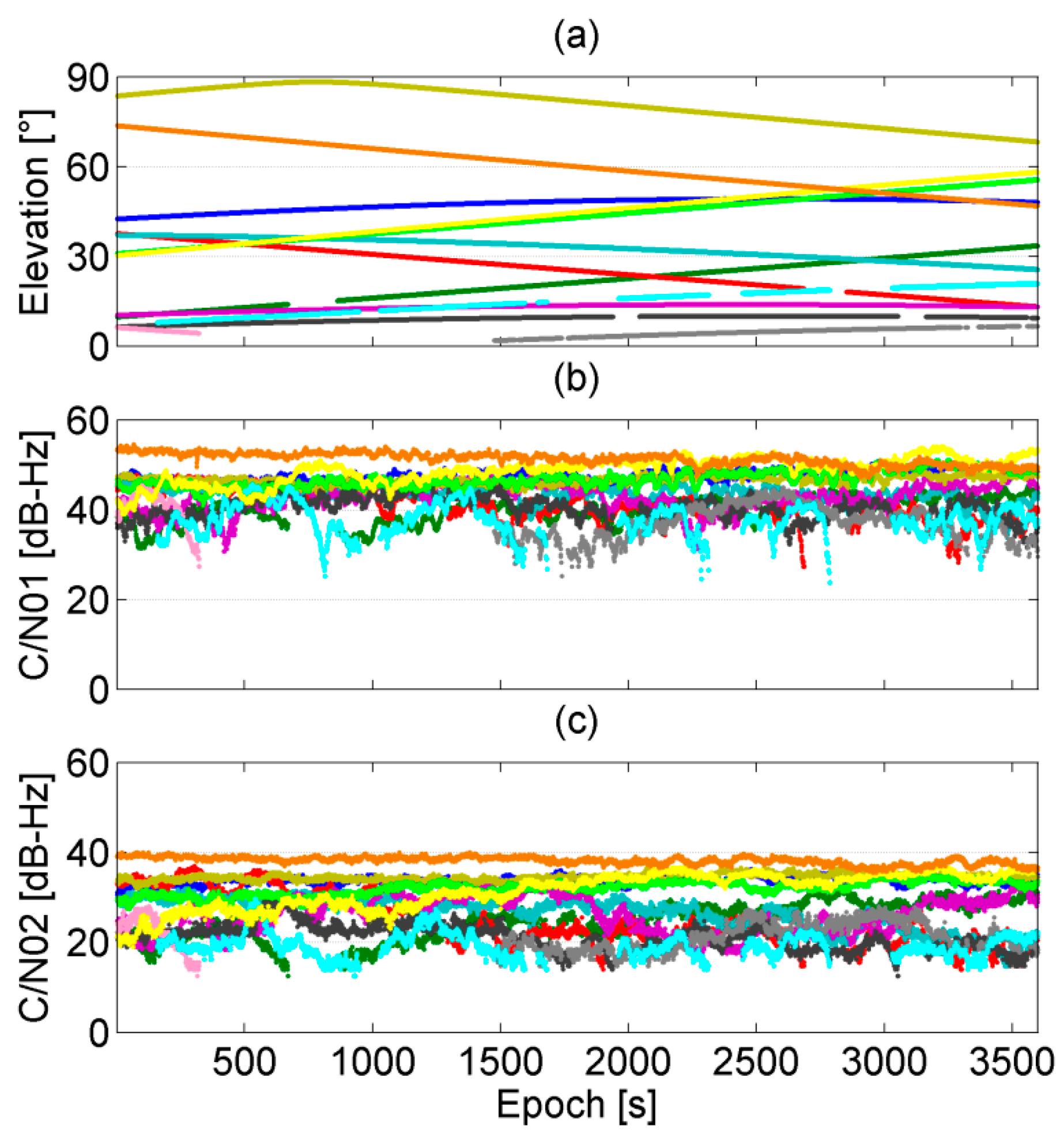
3. Data and Experiments

In this study, we tested a Trimble R10 with the antenna embedded in the receiver. It is manufactured by the Trimble company in Sunnyvale, California, USA. Firstly, the template functions of C/N0 and its precision are determined. As aforementioned, the template functions can be determined in advance for only once. The test receiver was placed on a permanent reference station, which was on the rooftop of the Engineering building (ENB) at the University of Calgary. In this situation, twenty-four hour dual frequency C/N0 observations on frequencies C1 and P2 with the sampling of 1 s were obtained from 00:00:00 to 23:59:59 on 24 November 2017 (GPS time). This ideal environment can help us to obtain the reliable reference nominal C/N0, then all the available Global Positioning System (GPS) satellites with 0 to 90 degrees can be tracked, as can be seen from the daily skyplot of visible satellites in Figure 1.

Secondly, in order to validate the effectiveness of the proposed method, two static and one kinematic experiments were carried out. To evaluate the performance of the proposed method, two types of code-based positioning are used. The first one is the SPP, where the ionospheric and tropospheric delays were corrected by the Klobuchar and Hopfield models, respectively. The second one is the RTD, where the ionosphere-fixed model [41] and the Hopfield model were applied. The reference station is UCAL (−1,641,945.119 m, −3,664,803.809 m, and 4,940,009.252 m, in WGS84 coordinate system) which is also located at the University of Calgary from the International GNSS Service [44]. Four types of weighting models are applied into the SPP and RTD for comparison: (A) the equal-weight model (EQUM) which assumes the variances of all the observations are equal; (B) the elevation model (ELEM) using Equation (4); (C) the C/N0 model (CN0M) using Equation (6); (D) the proposed adaptive model (ADAM) using Equation (16). For these four weighting models, to obtain the comparable results, the cut-off elevations are the same, and the scale factor $\beta$ of the ADAM is set to 2.

The first static experiment was carried out as dataset no. 1. We recorded 1-Hz GPS C1 and P2 data for consecutive 1 h from 19:00:00 to 19:59:59 on 25 November 2017 (GPS time). The coordinates of the test station are precisely known by applying the real-time kinematic positioning (RTK). When using the relative positioning, the baseline length is approximately 133 m. Figure 2 shows the environment of the test receiver placed nearby the blocks of ENB. It can be seen that the observation environment is like in a dense high-rise building group that could offer a variety of reflective multipath and NLOS reception, where the signals could be reflected and blocked by the ENB.

The second static experiment was carried out as dataset no. 2. One-hour GPS C1 and P2 observations with the sampling interval of 1 s were collected from 21:30:00 to 22:29:59 on 27 November 2018 (GPS time). The coordinates of the test station are precisely known by applying the RTK, and the baseline length is approximately 396 m when using the RTK and RTD. Figure 3 illustrates the test receiver deployed nearby the trees on the campus of University of Calgary. It is clear that the observation environment is like in a heavy urban-forested area where a variety of diffractive multipath, and even NLOS reception, occur, caused by the trees.

A kinematic experiment was then carried out as dataset no. 3. 1-Hz GPS C1 data was recorded in approximately consecutive 40 min from 19:58:33 to 20:38:23 on 26 November 2018 (GPS time). When using the RTD, the longest length of this kinematic baseline is less than 1 km. This kinematic experiment was deployed on the main road at the University of Calgary, as shown in Figure 4. It can be found that the observation environment could offer different situations during the test. Specifically, it is noted that the site-specific unmodeled errors will be significant when the test receiver is located between the Energy Environment Experiential Learning (EEEL) and Earth Science (ES) buildings, as shown in the left panel (a) of Figure 4 marked with yellow rectangle. These unmodeled effects can be further confirmed by the specific environments of EEEL and ES buildings (see the right panel (b) of Figure 4).

4. Results and Discussion

In this section, the template functions are analyzed firstly. After that, the results of the two static and one kinematic experiments are discussed, where the proposed model ADAM is compared with the other three traditional models EQUM, ELEM, and CN0M.

4.1. Template Functions

As aforementioned, the highly reliable template functions of the test receiver need to be determined. Firstly, the means and STDs of C/N0 values of each satellite (except for G04 due to outage) from elevations of 35 to 80 degrees are compared. The reason is that most external influences can be reduced above 35-degree elevations [27,43] and several satellites do not have the measurements above 80-degree elevations. Figure 5 illustrates the mean C/N0 on C1 and P2, as well as the one-time STD ranges of each satellite. It can be seen that the means and STDs are rather similar with each other, thus indicating that the same template functions can be used among all the GPS satellites. Secondly, the raw C/N0 observations are removed if the values exceed double STD ranges in each one-degree interval. Figure 6 shows the refined reference C/N0 of C1 (C/N01) and P2 (C/N02). It is clear that the reference measurements from different GPS satellites are elevation-dependent and consistent with each other, which can be fit by the third-order polynomials.

In the end, the template functions of C/N0 on two frequencies are determined by using Equation (9):

$$\mathrm{C}/\mathrm{N}{01}_{nom}\left(\theta \right)=37.79+0.2611\theta -6.044\times {10}^{-4}{\theta }^2-7.707\times {10}^{-6}{\theta }^3,$$

(17)

$$\mathrm{C}/\mathrm{N}{02}_{nom}\left(\theta \right)=18.12+0.5213\theta -4.302\times {10}^{-3}{\theta }^2+1.140\times {10}^{-5}{\theta }^3,$$

(18)

The template functions of C/N0 precision on these two frequencies can also be determined by the STDs of every 1-degree elevation interval by using Equation (10):

$${\mathrm{STD}}_{\mathrm{C}/\mathrm{N}{01}_{nom}}\left(\theta \right)=2.672-0.06788\theta +1.106\times {10}^{-3}{\theta }^2-5.317\times {10}^{-6}{\theta }^3,$$

(19)

$${\mathrm{STD}}_{\mathrm{C}/\mathrm{N}{02}_{nom}}\left(\theta \right)=3.310-0.07618\theta +9.216\times {10}^{-4}{\theta }^2-3.438\times {10}^{-6}{\theta }^3,$$

(20)

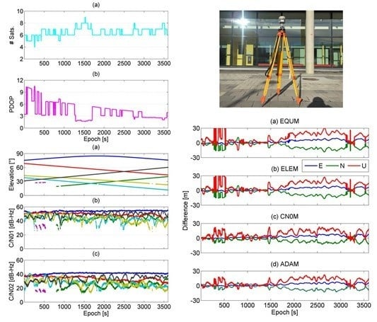
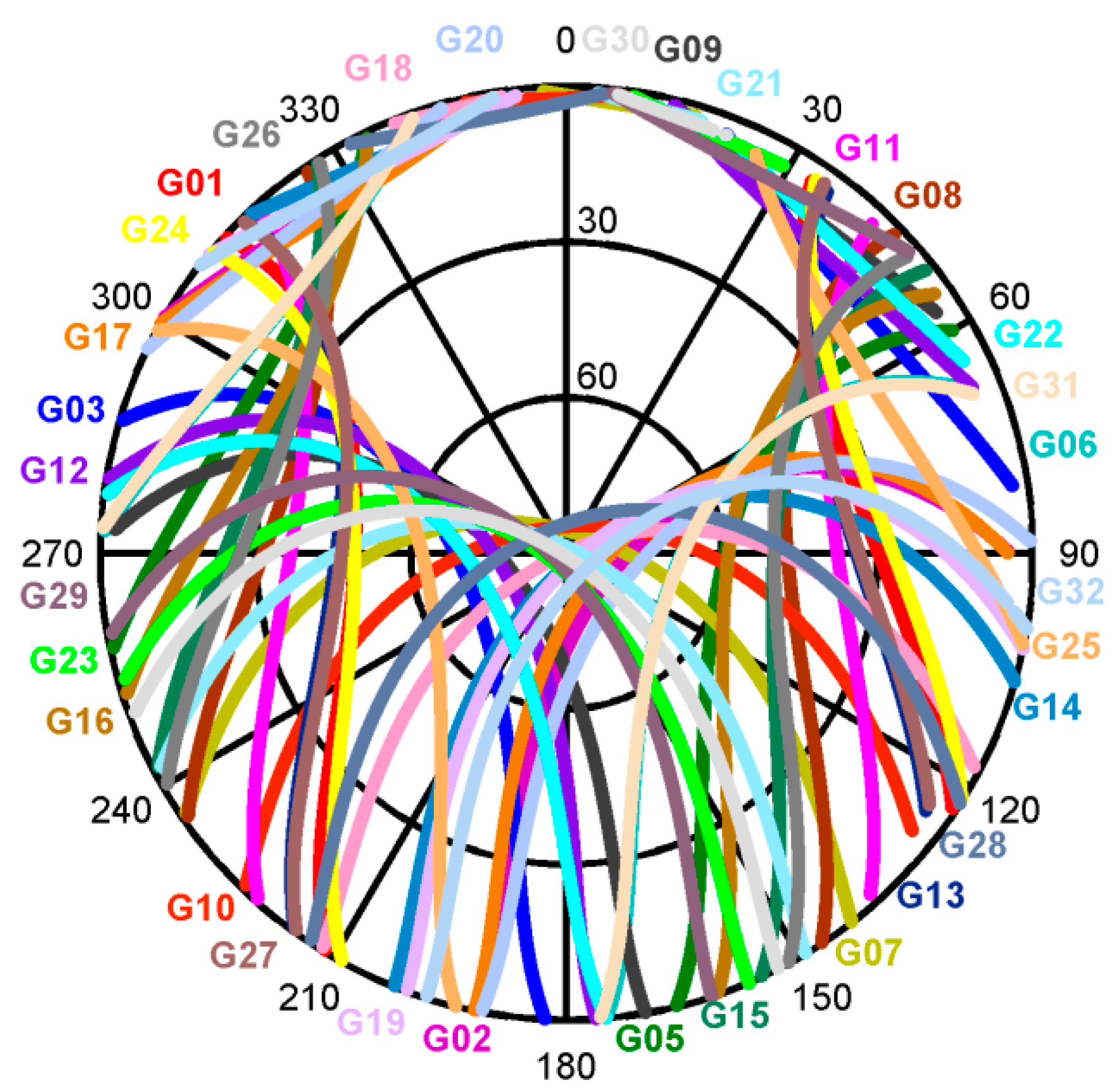
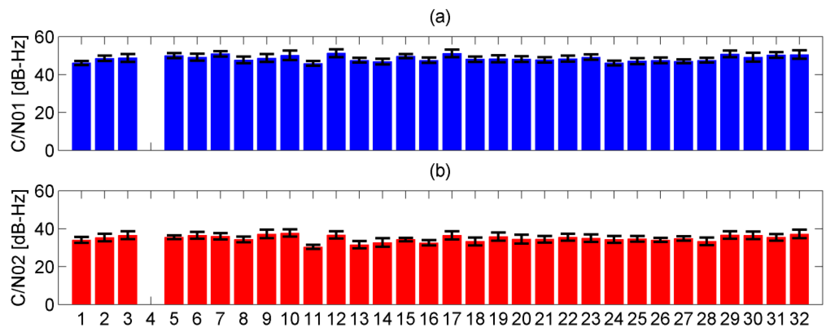
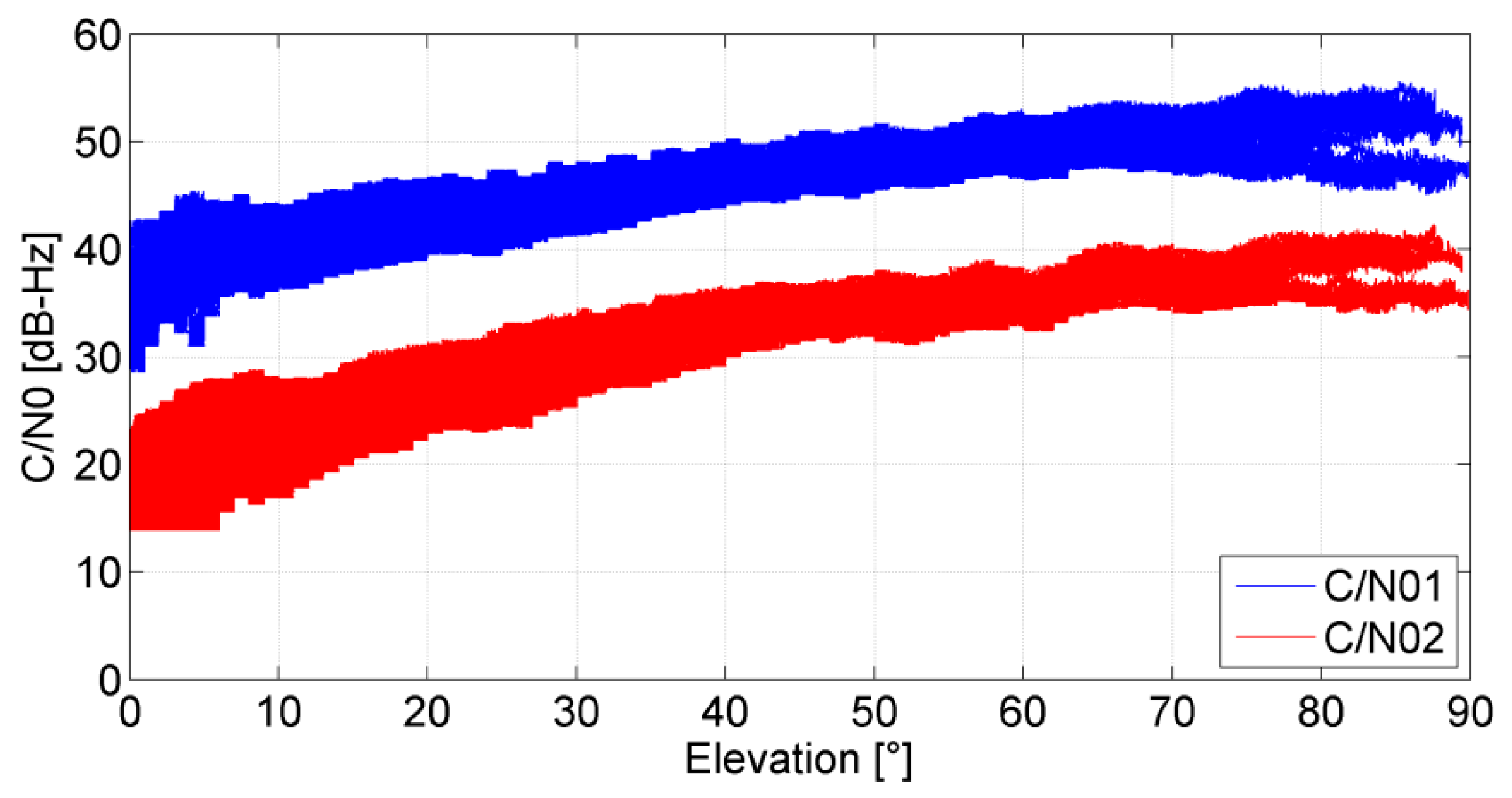
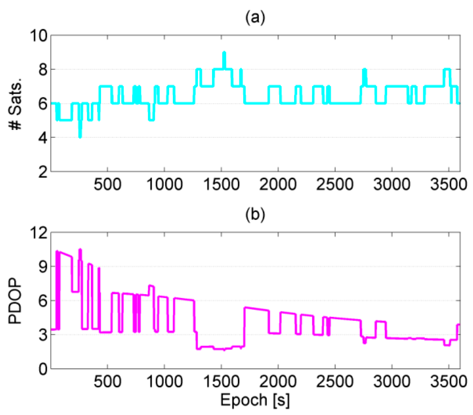
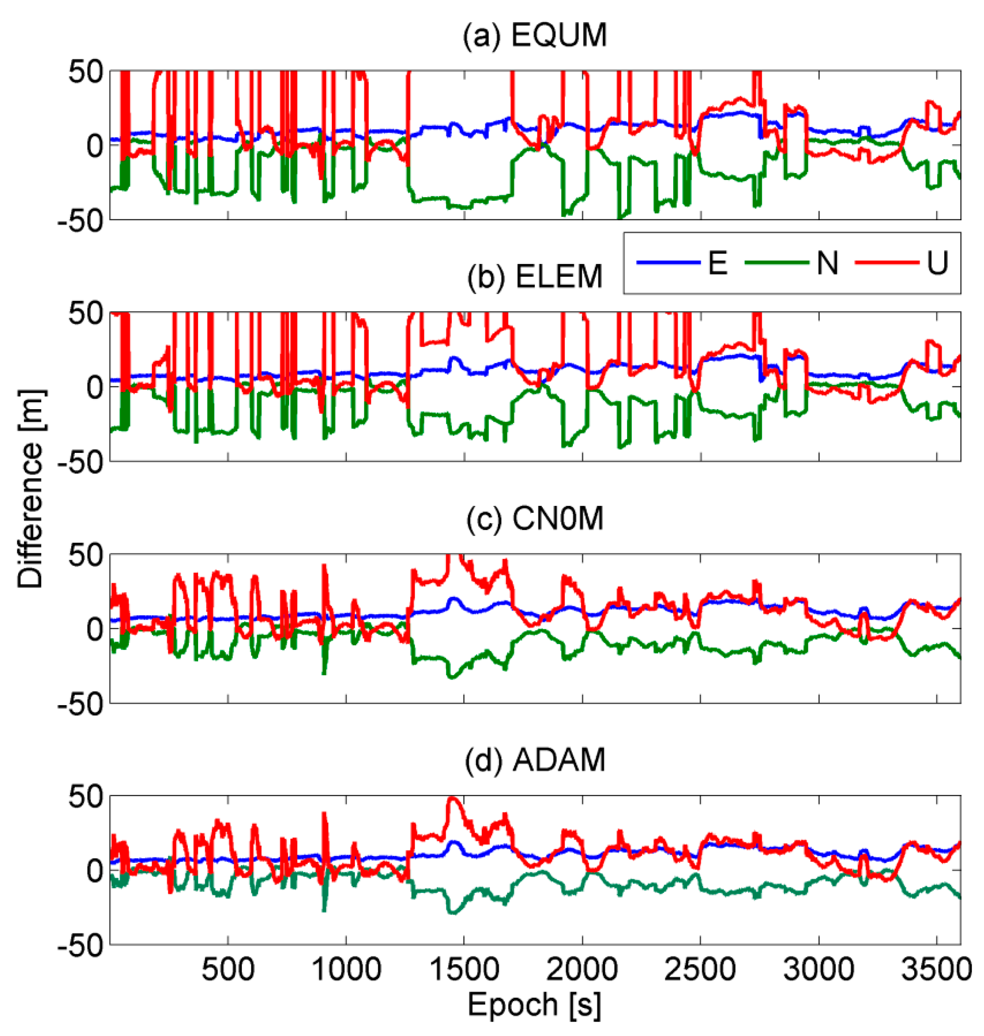
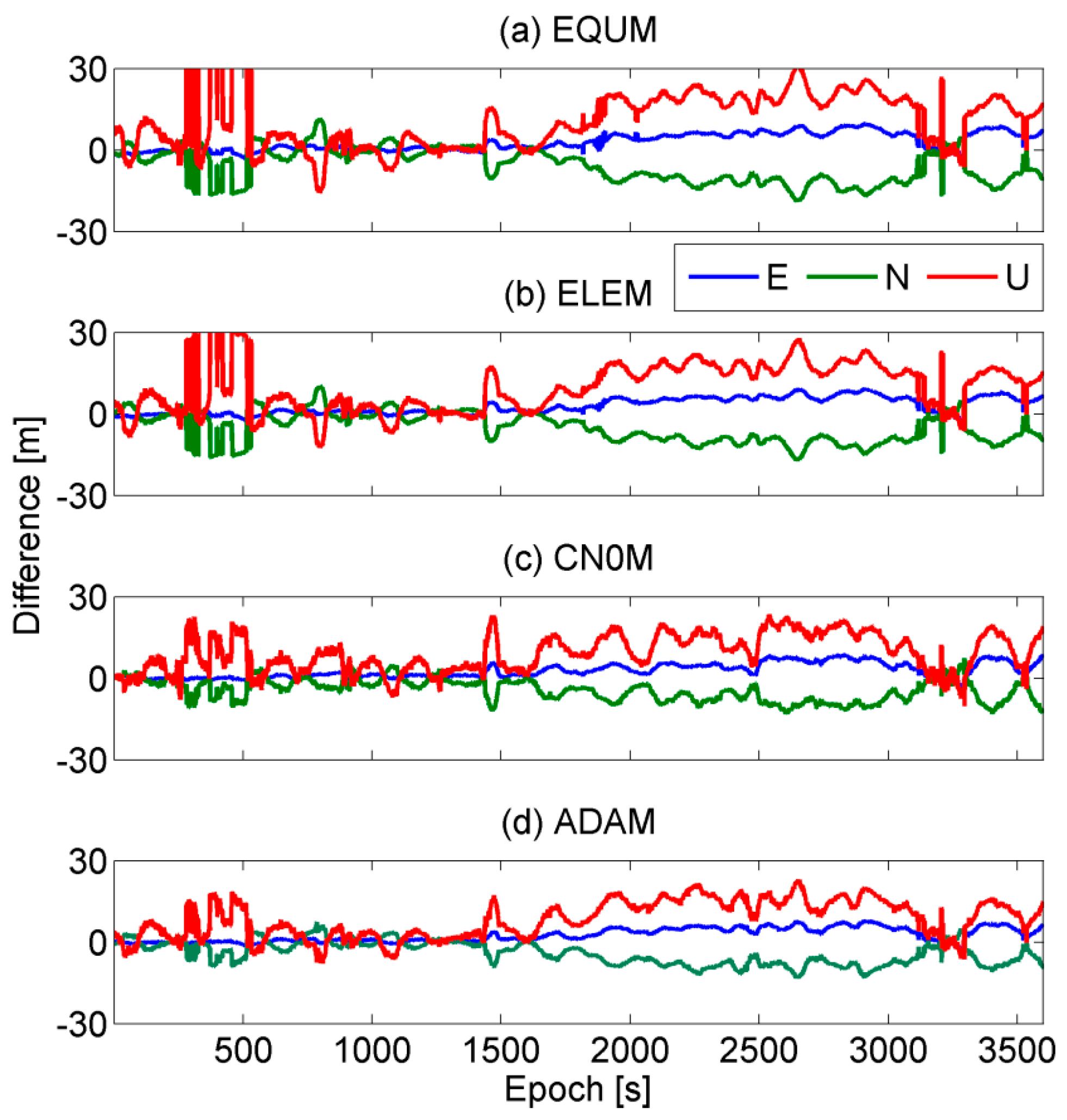
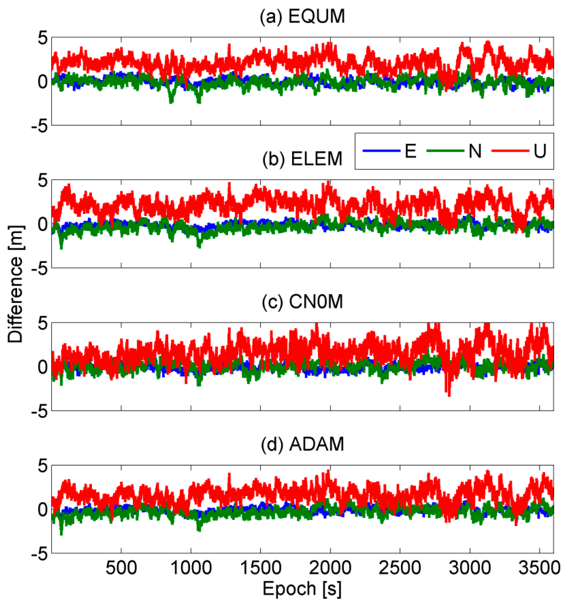
4.2. Static Experiment Near Buildings

The results of the first static experiment are shown here. In dataset no. 1, the averages of satellite numbers and positional dilution of precision (PDOP) values are 6.5 and 4.2, respectively, as shown in Figure 7. It can be used to further confirm the poor observation environment of dataset no. 1.

The positioning errors (relative to the known precise coordinates) of the single-frequency SPP results by using the EQUM, ELEM, CN0M, and ADAM are illustrated in Figure 8. The E, N, and U denote the east, north, and up directions, respectively. It can be clearly seen that the CN0M and ADAM perform much better than the other two models, especially for the first around 3000 epochs. One may conclude that the C/N0-dependent models (CN0M and ADAM) are necessary in challenging environments. Compared with the results of CN0M and ADAM, the ADAM is more precise. It indicates that, unlike the ADAM, the CN0M only indirectly and partly reflect the precisions of site-specific unmodeled errors. That is, the template functions in ADAM are, indeed, effective.

Table 1. Statistical results of SPP and RTD using the equal-weight model (EQUM), elevation model (ELEM), C/N0 model (CN0M), and adaptive model (ADAM). The RMS values of E, N, and U directions, and 3D RMS values were calculated from dataset no. 1 (m).

	SPP				RTD
	EQUM	ELEM	CN0M	ADAM	EQUM	ELEM	CN0M	ADAM
E	11.73	11.35	11.79	11.15	4.36	4.19	3.83	3.59
N	22.44	18.43	12.37	10.74	8.69	7.63	6.00	5.91
U	36.03	30.74	18.99	15.65	14.92	13.43	11.57	10.84
3D	44.04	37.59	25.55	22.01	17.81	16.00	13.58	12.86

presents the corresponding statistical results of SPP and RTD using the four types of weighting models. It can be confirmed that, compared with the SPP results of EQUM, ELEM, and CN0M, the three-dimensional root mean square (3D RMS) values of ADAM are improved by 50.0%, 41.4%, and 13.9%, respectively. The dual-frequency RTD results by using the four types of weighting models are illustrated in Figure 9. Similarly, it can be clearly seen that the proposed method is the most precise. According to the Table 1, the improvement percentages of the ADAM compared with the EQUM, ELEM, and CN0M are 27.8%, 19.6%, and 5.3%, respectively.

The reason why the ADAM is better than any other traditional methods is that the ADAM can mitigate these unmodeled effects greatly. Figure 10 illustrates the elevations and dual-frequency C/N0 of all the used satellites denoted with different colors. It can be seen that the C/N0 patterns are significantly different from the reference values in Figure 6. The reason is that several GPS signals suffer the multipath and even the NLOS reception due the blocks of ENB. In addition, it can also be found that the low elevations do not necessarily mean the low C/N0. It is reasonable since the observations with high elevations cannot ensure that they are free from the multipath and NLOS reception. Actually, this is why the positioning results of the ELEM and CN0M are significantly different with each other in this situation.

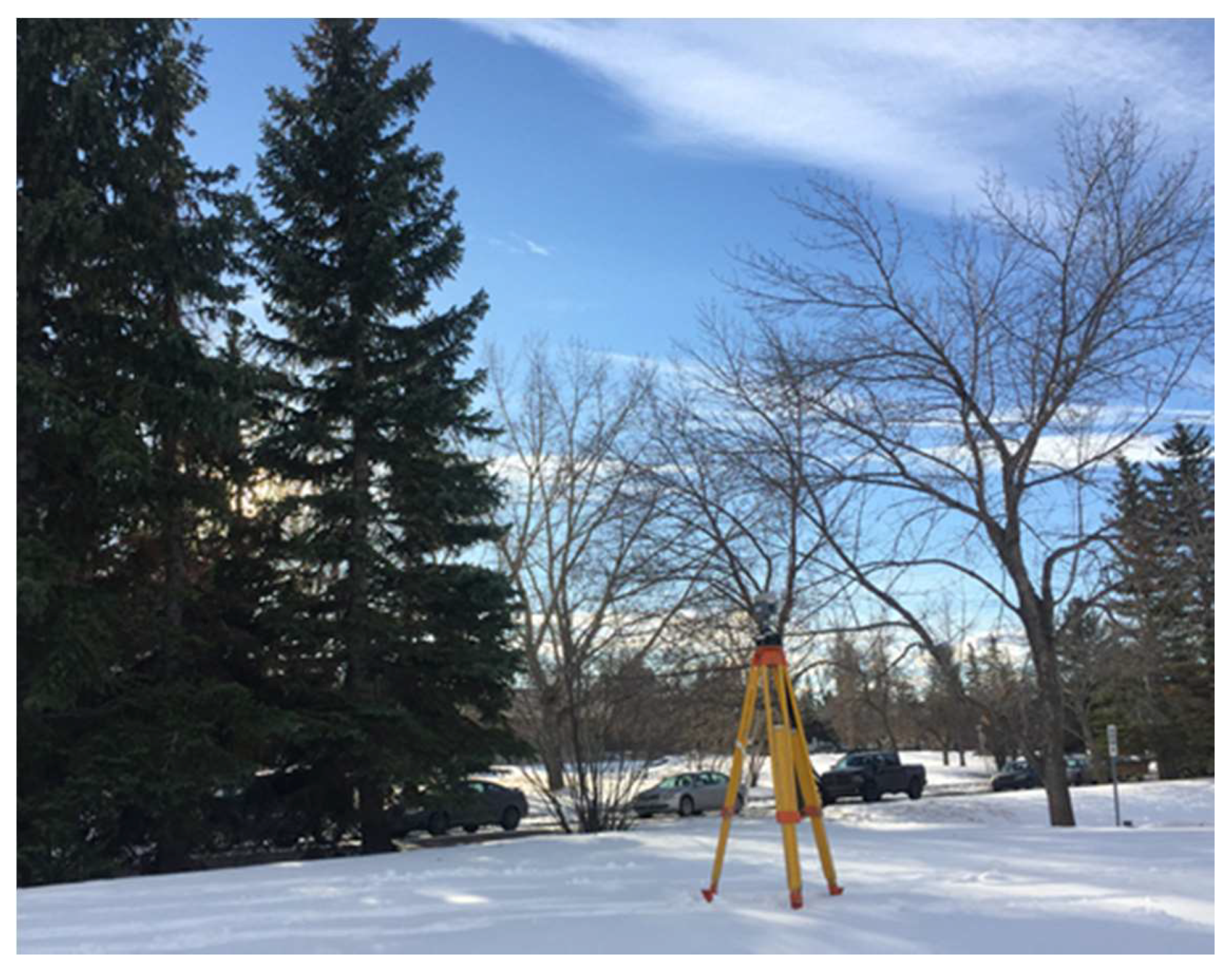
4.3. Static Experiment Near Trees

The results of the second static experiment are then discussed. In dataset no. 2, the averages of satellite numbers and PDOP values are 11.7 and 1.5, respectively, as shown in Figure 11. Therefore, compared with dataset no. 1, the proposed method can be evaluated in a relatively good observation condition.

The positioning errors of the single-frequency SPP results by using the EQUM, ELEM, CN0M, and ADAM are presented in Figure 12. It can be easily seen that the ADAM is still the most precise. Specifically, the accuracy of EQUM and CN0M are lower than those of ELEM and ADAM, particularly in the U direction. It indicates that the elevation is an indispensable indicator in some cases. Hence, it is necessary to use the elevation as the foundation part of the proposed model.

Table 2. Statistical results of SPP and RTD using the equal-weight model (EQUM), elevation model (ELEM), C/N0 model (CN0M), and adaptive model (ADAM). The RMS values of E, N, and U directions, and 3D RMS values were calculated from dataset no. 2 (m).

	SPP				RTD
	EQUM	ELEM	CN0M	ADAM	EQUM	ELEM	CN0M	ADAM
E	3.20	3.18	3.02	3.01	0.41	0.43	0.38	0.38
N	3.97	3.64	3.69	3.49	0.65	0.62	0.58	0.62
U	5.08	3.93	4.36	3.60	2.32	2.01	2.23	1.90
3D	7.20	6.23	6.46	5.85	2.44	2.15	2.34	2.03

gives the corresponding statistical results of SPP and RTD using the four types of weighting models. Compared with the SPP results of EQUM, ELEM, and CN0M, the 3D RMS values of ADAM are improved by 18.8%, 6.1%, and 9.4%, respectively. The dual-frequency RTD results by using the four types of weighting models are all shown in Figure 13. Once again, the proposed method is still the most precise. As shown in Table 2, the improvement percentages of the ADAM compared with the EQUM, ELEM and CN0M are 16.8%, 5.6%, and 13.2%, respectively.

Taking a closer look at the SPP results of the ELEM and ADAM, the ADAM can also eliminate the spikes around 2350 s, whereas the ELEM cannot. One may conclude that the ADAM can adjust the precisions of the site-specific unmodeled errors adaptively, since the site-specific unmodeled errors may become significant around 2350 s. It can be confirmed by the elevations and C/N0 of the satellite denoted with the cyan color in Figure 14, which illustrates the elevations and dual-frequency C/N0 of all the used satellites. Specifically, the satellite denoted by the cyan color has a minimum C/N0 around 2350 s, whereas its elevations are not a minimum. In conclusion, the other advantage of the proposed method is that it can adaptively mitigate the spikes of the positioning results.

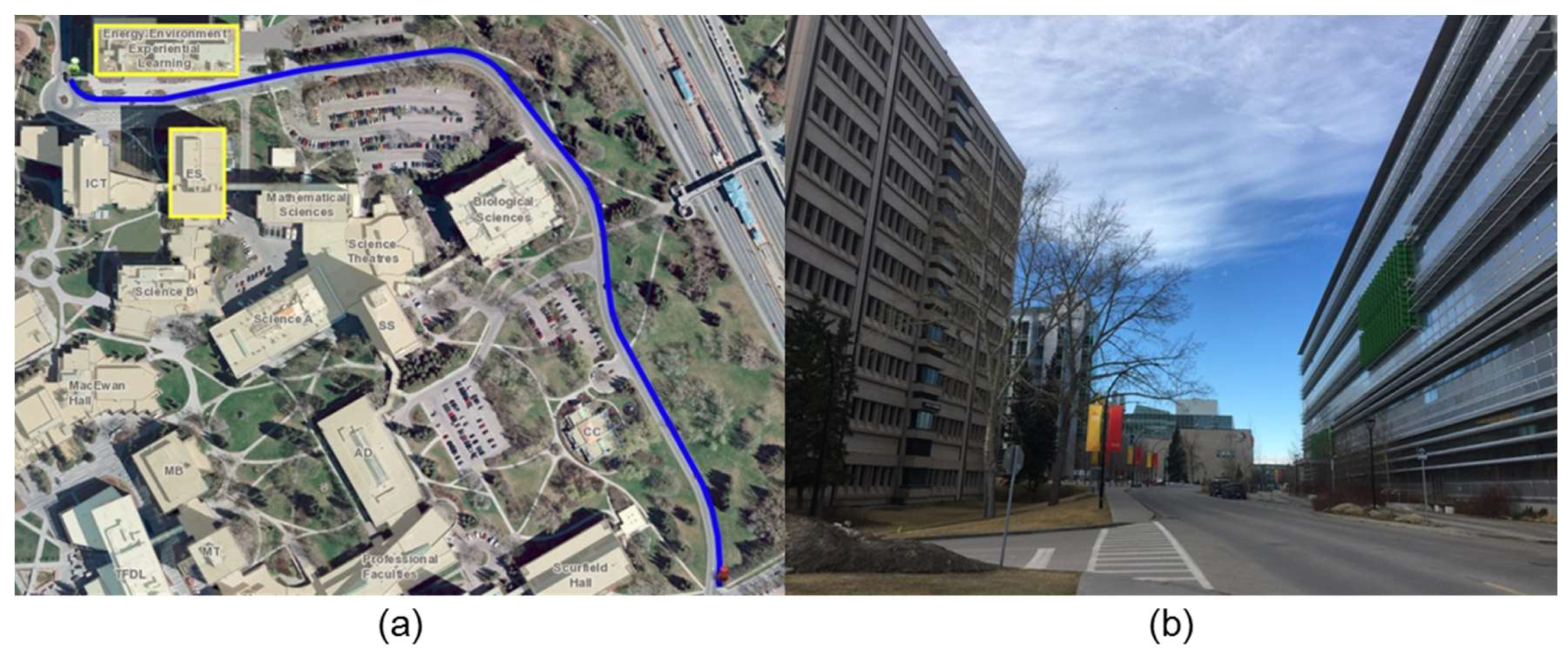
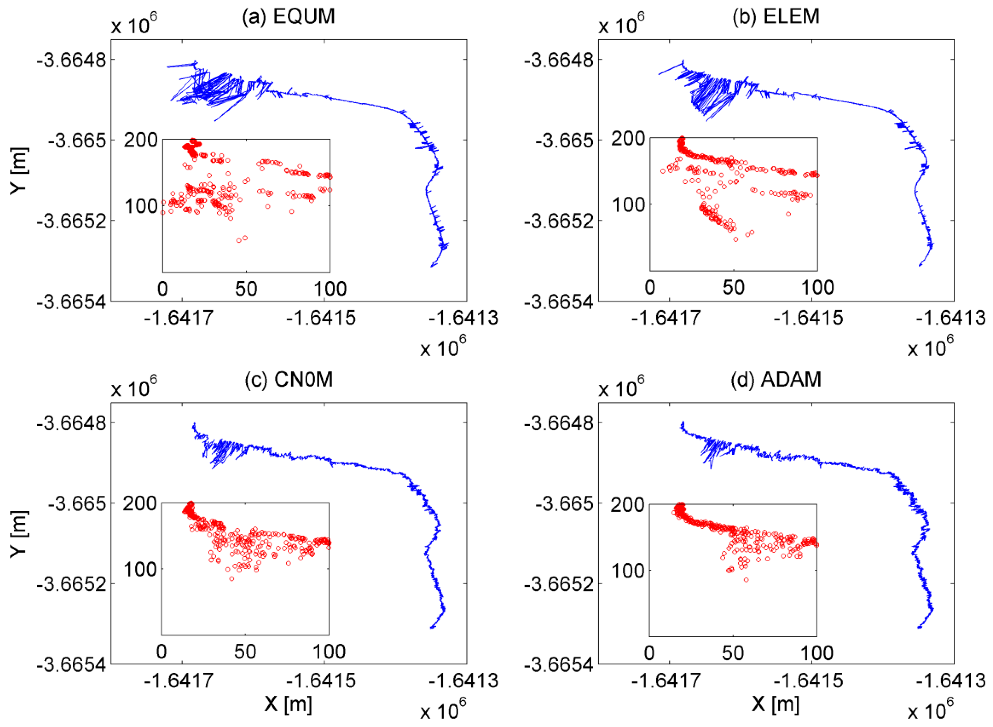
4.4. Kinematic Experiment

In the end, we present the results of the kinematic experiment. Figure 15 illustrates the satellite numbers and PDOP values calculated from dataset no. 3. It is clear that between around 150 and 500 s, the satellite numbers become fewer and the PDOP values become larger. As aforementioned, this is because the test receiver is located between the EEEL and ES buildings at this time and several GPS signals are obstructed. It also indicates that the multipath and NLOS reception inevitably exist in some other GPS signals at this time. The SPP results by using the EQUM, ELEM, CN0M, and ADAM are illustrated in Figure 16. Since this experiment was carried out in Calgary, the X and Y coordinates in the WGS84 coordinate system are all negative. Compared with the other models, the ADAM is the most precise, especially when the test receiver is between EEEL and ES buildings. It can be further confirmed by the small panels of each subplot from Figure 16. The RTD results by using the four types of weighting models are illustrated in Figure 17. Once again, the proposed method is the most precise, like in Figure 16. Actually, the reason is that the observations contaminated by the site-specific unmodeled errors are adaptively down-weighted by the ADAM. In conclusion, it demonstrates that the proposed method can mitigate the site-specific unmodeled errors to a great extent in kinematic modes regardless of SPP or RTD solutions, and has a great potential in urban canyon areas.

5. Conclusions

In this paper, we developed a new real-time adaptive weighting model which can mitigate the site-specific unmodeled errors of undifferenced code observations. The proposed method combines the elevation and C/N0, where the precision of the receiver noise and atmospheric delay are described by the elevation, and the precision of site-specific unmodeled error is described by the C/N0. Unlike the traditional C/N0 models, the template functions of C/N0 and its precision are applied to adaptively estimate the precisions of site-specific unmodeled errors.

The effectiveness of the adaptive weighting model is validated by the static and kinematic experiments. For the static experiment near buildings, the 3D RMS of the proposed model are improved by 35.1% and 17.6% on average compared with the other traditional models. It can be found that the observations with high elevations cannot ensure large C/N0 values in difficult environments. Additionally, the results indicate that the traditional C/N0-based model only indirectly and partly reflect the precisions of site-specific unmodeled errors. However, by taking full advantage of the template functions that can estimate the nominal values, the proposed method can mitigate these unmodeled effects to a great extent. For the static experiment near trees, 11.4% and 11.9% of improvements are obtained by using the proposed model compared with the other traditional models. The results indicate that it is necessary to use the elevation as the foundation part of the proposed model. In addition, the other advantage of the proposed model is that it can adaptively mitigate the spikes of the positioning results. For the kinematic experiment, the proposed model is also effective since the observations contaminated by the site-specific unmodeled errors can be down-weighted adaptively.

In conclusion, the SPP and RTD results show that the adaptive model is superior to the conventional equal-weight, elevation and C/N0 models especially in challenging environments, such as dense high-rise building group and urban-forested area. It is worth noting that the effectiveness of the proposed weighting model relies on the precisions of template functions of used receiver. Specifically, when the precisions of template functions are high, the proposed weighting model can mitigate the site-specific unmodeled effects even if they are not very severe. On the contrary, when the precisions of template functions are low, the proposed weighting model is not very sensitive to these unmodeled effects even if they are severe. At last, in GNSS precise positioning, this new model is an important supplementary for the theory of GNSS unmodeled error processing and can be easily used to extend the elevation-based weighting model in GNSS positioning programs.

References

1. Li, T.; Zhang, H.; Gao, Z.; Chen, Q.; Niu, X. High-accuracy positioning in urban environments using single-frequency multi-GNSS RTK/MEMS-IMU integration. Remote Sens. 2018, 10, 205. [Google Scholar] [CrossRef]
2. Cai, C.; Pan, L.; Gao, Y. A precise weighting approach with application to combined L1/B1 GPS/BeiDou positioning. J. Navig. 2014, 67, 911–925. [Google Scholar] [CrossRef]
3. Hsu, L.; Jan, S.; Groves, P.; Kubo, N. Multipath mitigation and NLOS detection using vector tracking in urban environments. GPS Solut. 2015, 19, 249–262. [Google Scholar] [CrossRef]
4. Zhang, Z.; Li, B.; Shen, Y. Comparison and analysis of unmodelled errors in GPS and BeiDou signals. Geodesy Geodyn. 2017, 8, 41–48. [Google Scholar] [CrossRef]
5. Li, B.; Zhang, Z.; Shen, Y.; Yang, L. A procedure for the significance testing of unmodeled errors in GNSS observations. J. Geodesy 2018, 1–16. [Google Scholar] [CrossRef]
6. Pietrantonio, G.; Riguzzi, F. Three-dimensional strain tensor estimation by GPS observations: Methodological aspects and geophysical applications. J. Geodyn. 2004, 38, 1–18. [Google Scholar] [CrossRef]
7. Shu, Y.; Fang, R.; Liu, J. Stochastic Models of Very High-Rate (50 Hz) GPS/BeiDou Code and Phase Observations. Remote Sens. 2017, 9, 1188. [Google Scholar] [Green Version]
8. Koch, K. Parameter Estimation and Hypothesis Testing in Linear Models; Springer: Berlin, Germany, 1999. [Google Scholar]
9. Li, B.; Shen, Y.; Lou, L. Efficient estimation of variance and covariance components: A case study for GPS stochastic model evaluation. Geosci. Remote Sens. IEEE Trans. 2011, 49, 203–210. [Google Scholar] [CrossRef]
10. Baarda, W. A Testing Procedure for Use in Geodetic Networks; Rijkscommissie voor Geodesie: Kanaalweg 4, Delft, The Netherlands, 1968. [Google Scholar]
11. Teunissen, P. Testing Theory: An Introduction; VSSD: Delft, The Netherlands, 2000. [Google Scholar]
12. Bischoff, W.; Heck, B.; Howind, J.; Teusch, A. A procedure for testing the assumption of homoscedasticity in least squares residuals: A case study of GPS carrier-phase observations. J. Geodesy 2005, 78, 397–404. [Google Scholar] [CrossRef]
13. Euler, H.; Goad, C. On optimal filtering of GPS dual frequency observations without using orbit information. Bull. Géodésique 1991, 65, 130–143. [Google Scholar] [CrossRef]
14. King, R.; Bock, Y. Documentation for the GAMIT GPS Analysis Software; Massachusetts Institute of Technology: Cambridge, MA, USA, 2000; Available online: http://www-gpsg.mit.edu/~simon/gtgk/GAMIT.pdf (accessed on 24 June 2018).
15. Dach, R.; Hugentobler, U.; Fridez, P.; Meindl, M. Bernese GPS Software, version 5.0; Astronomical Institute, University of Bern: Bern, Switzerland, 2007. [Google Scholar]
16. Amiri-Simkooei, A.; Teunissen, P.; Tiberius, C. Application of least-squares variance component estimation to GPS observables. J. Surv. Eng. 2009, 135, 149–160. [Google Scholar] [CrossRef]
17. Li, B.; Zhang, L.; Verhagen, S. Impacts of BeiDou stochastic model on reliability: Overall test, w-test and minimal detectable bias. GPS Solut. 2017, 21, 1095–1112. [Google Scholar] [CrossRef]
18. Axelrad, P.; Comp, C.; Macdoran, P.F. SNR-based multipath error correction for GPS differential phase. IEEE Trans. Aerosp. Electron. Syst. 1996, 32, 650–660. [Google Scholar] [CrossRef]
19. Bilich, A.; Larson, K. Mapping the GPS multipath environment using the signal-to-noise ratio (SNR). Radio Sci. 2007, 43, 3442–3446. [Google Scholar] [CrossRef]
20. Lau, L.; Cross, P. A new signal-to-noise-ratio based stochastic model for GNSS high-precision carrier phase data processing algorithms in the presence of multipath errors. In Proceedings of the ION GNSS 2006, Fort Worth, TX, USA, 26–29 September 2006; pp. 276–285. [Google Scholar]
21. Talbot, N. Optimal weighting of GPS carrier phase observations based on the signal-to-noise ratio. In Proceedings of the International Symposia on Global Positioning Systems, Gold Coast, Queensland, Australia, 17–19 October 1998. [Google Scholar]
22. Brunner, F.; Hartinger, H.; Troyer, L. GPS signal diffraction modelling: The stochastic SIGMA-Δ model. J. Geodesy 1999, 73, 259–267. [Google Scholar] [CrossRef]
23. Hartinger, H.; Brunner, F. Variances of GPS phase observations: The SIGMA-ε model. GPS Solut. 1999, 2, 35–43. [Google Scholar] [CrossRef]
24. Wieser, A.; Brunner, F. An extended weight model for GPS phase observations. Earth Planets Space 2000, 52, 777–782. [Google Scholar] [CrossRef] [Green Version]
25. de Bakker, P.; Tiberius, C.; van der Marel, H.; van Bree, R. Short and zero baseline analysis of GPS L1 C/A, L5Q, GIOVE E1B, and E5aQ signals. GPS Solut. 2012, 16, 53–64. [Google Scholar] [CrossRef]
26. Li, B. Stochastic modeling of triple-frequency BeiDou signals: Estimation, assessment and impact analysis. J. Geodesy 2016, 90, 593–610. [Google Scholar] [CrossRef]
27. Zhang, Z.; Li, B.; Shen, Y.; Yang, L. A noise analysis method for GNSS signals of a standalone receiver. Acta Geod. Geophys. 2017, 52, 301–316. [Google Scholar] [CrossRef]
28. Luo, X.; Mayer, M.; Heck, B.; Awange, J. A Realistic and Easy-to-Implement Weighting Model for GPS Phase Observations. IEEE Trans. Geosci. Remote Sens. 2014, 52, 6110–6118. [Google Scholar] [CrossRef]
29. Yu, W.; Chen, B.; Dai, W.; Luo, X. Real-Time Precise Point Positioning Using Tomographic Wet Refractivity Fields. Remote Sens. 2018, 10, 928. [Google Scholar] [CrossRef]
30. Comp, C.; Axelrad, P. Adaptive SNR-based carrier phase multipath mitigation technique. IEEE Trans. Aerosp. Electron. Syst. 1998, 34, 264–276. [Google Scholar] [CrossRef]
31. Braasch, M. Multipath. In Springer Handbook of Global Navigation Satellite Systems; Springer: Berlin, Germany, 2017; pp. 443–468. [Google Scholar]
32. Bilich, A.; Larson, K.; Axelrad, P. Modeling GPS phase multipath with SNR: Case study from the Salar de Uyuni, Boliva. J. Geophys. Res. Solid Earth 2008, 113. [Google Scholar] [CrossRef] [Green Version]
33. Groves, P.; Jiang, Z.; Rudi, M.; Strode, P. A Portfolio Approach to NLOS and Multipath Mitigation in Dense Urban Areas. In Proceedings of the 26th International Technical Meeting of the Satellite Division of the Institute of Navigation (ION GNSS+ 2013), Nashville, TN, USA, 16–20 September 2013; pp. 3231–3247. [Google Scholar]
34. Strode, P.; Groves, P. GNSS multipath detection using three-frequency signal-to-noise measurements. GPS Solut. 2016, 20, 399–412. [Google Scholar] [CrossRef]
35. Lau, L.; Cross, P. Development and testing of a new ray-tracing approach to GNSS carrier-phase multipath modelling. J. Geodesy 2007, 81, 713–732. [Google Scholar] [CrossRef]
36. Moradi, R.; Schuster, W.; Feng, S.; Jokinen, A.; Ochieng, W. The carrier-multipath observable: A new carrier-phase multipath mitigation technique. GPS Solut. 2014, 19, 73–82. [Google Scholar] [CrossRef]
37. Kaplan, E.; Hegarty, C. Understanding GPS: Principles and Applications; Artech House: Norwood, MA, USA, 2006. [Google Scholar]
38. Misra, P.; Enge, P. Global Positioning System: Signals, Measurements, and Performance; Ganga-Jamuna Press: Lincoln, MA, USA, 2012. [Google Scholar]
39. Klobuchar, J. Ionospheric time-delay algorithm for single-frequency GPS users. IEEE Trans. Aerosp. Electron. Syst. 1987, 325–331. [Google Scholar] [CrossRef]
40. Hopfield, H. Two-quartic tropospheric refractivity profile for correcting satellite data. J. Geophys. Res. Atmos. 1969, 74, 4487–4499. [Google Scholar] [CrossRef]
41. Odijk, D. Weighting ionospheric corrections to improve fast GPS positioning over medium distances. In Proceedings of the ION GPS, Salt Lake City, UT, USA, 19–22 September 2000; pp. 1113–1123. [Google Scholar]
42. Lau, L.; Cross, P. Investigations into phase multipath mitigation techniques for high precision positioning in difficult environments. J. Navig. 2007, 60, 457–482. [Google Scholar] [CrossRef]
43. Bona, P. Precision, cross correlation, and time correlation of GPS phase and code observations. GPS Solut. 2000, 4, 3–13. [Google Scholar] [CrossRef]
44. Dow, J.; Neilan, R.; Rizos, C. The international GNSS service in a changing landscape of global navigation satellite systems. J. Geodesy 2009, 83, 191–198. [Google Scholar] [CrossRef]
Figure 1. Twenty-four hour skyplot of visible GPS satellites observed from the permanent reference station.
Remotesensing 10 01157 g001
Figure 2. Observation environment of dataset no. 1 near buildings.
Remotesensing 10 01157 g002
Figure 3. Observation environment of dataset no. 2 near trees.
Remotesensing 10 01157 g003
Figure 4. (a) Trajectory of dataset no. 3 represented as a blue line on the main road at the University of Calgary, where the EEEL and ES buildings are marked with yellow rectangles. The green and red points denote the starting point and finishing point, respectively; and (b) the test environment between the EEEL and ES buildings.
Remotesensing 10 01157 g004
Figure 5. Mean C/N0 values of each satellite, where the error bars are the one-time STD ranges for each satellite. (a) C/N0 of C1 (C/N01); and (b) C/N0 of P2 (C/N02).
Remotesensing 10 01157 g005
Figure 6. Refined reference C/N0 of C1 (C/N01) and P2 (C/N02) as a function of elevation.
Remotesensing 10 01157 g006
Figure 7. (a) Satellite numbers; and (b) PDOP values. The data are calculated from the C1 observations of dataset no. 1.
Remotesensing 10 01157 g007
Figure 8. Positioning differences between the SPP solutions and the precise coordinates of dataset no. 1. (a) Results of the equal-weight model (EQUM); (b) results of the elevation model (ELEM); (c) results of the C/N0 model (CN0M); and (d) results of the adaptive model (ADAM).
Remotesensing 10 01157 g008
Figure 9. Positioning differences between the RTD solutions and the precise coordinates of dataset no. 1. (a) Results of the equal-weight model (EQUM); (b) results of the elevation model (ELEM); (c) results of the C/N0 model (CN0M); and (d) results of the adaptive model (ADAM).
Remotesensing 10 01157 g009
Figure 10. (a) Elevations of used satellites; (b) C/N0 of C1 (CN01) of used satellites; and (c) C/N0 of P2 (CN02) of used satellites. Each color denotes one satellite calculated from dataset no. 1.
Remotesensing 10 01157 g010
Figure 11. (a) Satellite numbers; and (b) PDOP values. The data are calculated from the C1 observations of dataset no. 2.
Remotesensing 10 01157 g011
Figure 12. Positioning differences between the SPP solutions and the precise coordinates of dataset no. 2. (a) Results of the equal-weight model (EQUM); (b) results of the elevation model (ELEM); (c) results of the C/N0 model (CN0M); and (d) results of the adaptive model (ADAM).
Remotesensing 10 01157 g012
Figure 13. Positioning differences between the RTD solutions and the precise coordinates of dataset no. 2. (a) Results of the equal-weight model (EQUM); (b) results of the elevation model (ELEM); (c) results of the C/N0 model (CN0M); and (d) results of the adaptive model (ADAM).
Remotesensing 10 01157 g013
Figure 14. (a) Elevations of used satellites; (b) C/N0 of C1 (CN01) of used satellites; and (c) C/N0 of P2 (CN02) of used satellites. Each color denotes one satellite calculated from dataset no. 2.
Remotesensing 10 01157 g014
Figure 15. (a) Satellite numbers; and (b) PDOP values. The data are calculated from dataset no. 3.
Remotesensing 10 01157 g015
Figure 16. SPP results (blue lines) of dataset no. 3, where the horizontal and vertical coordinates denote the X and Y directions in WGS84 coordinate system respectively, and the detailed results (red points) in meter when the test receiver is located between EEEL and ES buildings. (a) Results of the equal-weight model (EQUM); (b) results of the elevation model (ELEM); (c) results of the C/N0 model (CN0M); and (d) results of the adaptive model (ADAM).
Remotesensing 10 01157 g016
Figure 17. RTD results (blue lines) of dataset no. 3, where the horizontal and vertical coordinates denote the X and Y directions in WGS84 coordinate system respectively, and the detailed results (red points) in meter when the test receiver is located between EEEL and ES buildings. (a) Results of the equal-weight model (EQUM); (b) results of the elevation model (ELEM); (c) results of the C/N0 model (CN0M); and (d) results of the adaptive model (ADAM).
Remotesensing 10 01157 g017