1. Introduction
In the last few years, a new approach to GNSS seismology, called VADASE, was developed [
1,
2]. VADASE is able to estimate in real time the velocities and displacements in a global reference frame (ITRF), using high-rate (1 Hz or more) carrier phase observations and broadcast products (orbits, clocks) collected by a stand-alone GNSS receiver, achieving a displacements accuracy within 1–2 cm (usually better) over intervals up to a few minutes. In this respect, the VADASE solution can be achieved in real time even on-board the GNSS receiver. Therefore, VADASE is able to supply in real time displacements and waveforms induced by an earthquake with an accuracy until now achievable only by seismometers or by two other well-established GNSS approaches: Precise Point Positioning (PPP) and Differential Positioning (DP).
Nevertheless, all these already available techniques to estimate coseismic displacements display some drawbacks. Seismometers are affected by saturation when they are close to strong earthquake epicenters. Moreover, both GNSS-based approaches have some restrictions: PPP achieves an accuracy of a few millimeters, but it requires additional precise products (orbits, clocks and Earth orientation parameters); DP guarantees the real-time solution only if all the GNSS receivers are continuously connected in a permanent station network and their data are processed in real time by a centralized analysis center according to a differential approach. Furthermore, in the case of strong earthquakes affecting the entire area covered by the GNSS permanent network, DP is not able to supply coseismic displacements and waveforms in the global reference frame, since no stable reference stations are available.
VADASE is able to overcome the above-mentioned limitations, since GNSS solutions do not clip even in the case of strong ground shakings, and neither additional products, nor reference stations are required. Anyway, since the very first implementation and testing of VADASE, it was noticed that the estimated displacements may be impacted by two different effects: spurious spikes in the velocities due to outliers, so that displacements, obtained through velocities integration, are severely corrupted; trends in the displacements time series, mainly due to broadcast orbit and clock errors.
Two strategies are herein introduced to solve these issues, respectively based on Leave-One-Out cross-validation [
3] (VADASE-LOO) for a receiver autonomous outlier detection and on a network augmentation strategy to filter common trends out (A-VADASE); they are combined (first, VADASE-LOO; second, A-VADASE) for a complete solution (A-VADASE-LOO). Moreover, starting from this VADASE improved solution, an additional strategy is proposed to estimate in real time the overall coseismic displacement occurring at each GNSS receiver; this is based on the hypothesis of a constant mean level noise of the VADASE velocity estimates over a few minutes (just before, during and just after the earthquake) and on a robust estimation procedure.
An application of this VADASE improved solution and the real-time coseismic displacement estimations is herein presented for three relevant earthquakes that occurred in Central Italy in 2016 (
6.0, 24 August 2016, 01:36:54 (UTC),
5.9, 26 October 2016, 19:18:08 (UTC),
6.5, 30 October 2016, 06:40:19 (UTC)). In
Section 2.1 and
Section 2.2, VADASE-LOO and A-VADASE are described; in
Section 2.3, their application to Central Italy earthquakes is discussed; in
Section 3, the validation of the strategy for the real-time estimation of coseismic displacements with respect to the same earthquakes is given; finally, in
Section 4, some conclusions are outlined.
2. VADASE Improved Solution
2.1. VADASE Leave-One-Out
The real-time VADASE solutions can be impacted by spurious oscillations in the estimated velocities, due to outliers in GNSS observations, resulting in false displacements [
4]. A strategy to detect these outliers in real-time is defined on the basis of the Leave-One-Out Cross-Validation (LOOCV) approach; for technical details about this method, please refer to [
3,
5] As a matter of fact, standard techniques for outlier detection, as the well-known Baarda data snooping [
6], are not able to supply statistical tests of suitable power in the case of low redundancy, which often may happen in the VADASE real-time epoch-by-epoch solution due to the limited number of satellites in view in the two considered consecutive epochs. On the contrary, LOOCV can overcome this problem, since one observation is tested for a possible outlier at each time, but this is achieved at the cost of
n-repeated least squares epoch-by-epoch solutions (
n being the number of satellites in view in the two considered consecutive epochs).
Therefore, if
n is the number of variometric equations, where the number of the sets of equations depends on the number of satellites common to the two epochs, the Leave-One-Out (LOO) method applied to the VADASE algorithm involves the repeated application of the algorithm using all the satellites except one, different in each iteration. The satellite left out is considered an outlier if the index
is out of the
t-Student distribution at the 5% significance level (see the
Appendix). LOOCV is however still feasible from the computational point of view (VADASE-LOO), since all the
n-repeated least squares epoch-by-epoch solutions with up to 10–12 satellites take one millisecond on a standard PC processor (e.g., CPU Xeon, 3.30 GHz and 16 GB RAM); therefore, such a processing appears certainly feasible even in the case of a high observation rate (e.g., 50 Hz).
The benefit of VADASE-LOO to detect and eliminate the outliers was preliminary demonstrated through its application to the observations collected at M0SE IGS permanent station (Rome, Italy) over 67 days (3 February–9 April 2016) (
Table 1). To compute the number of outliers, the 3D velocity variometric solutions obtained using VADASE and VADASE-LOO were considered; they were compared to a threshold value based on the noise (standard deviation
) of the velocities estimated in an undisturbed setting; in detail, this noise was estimated over four days of solutions at the M0SE permanent station, and the threshold was chosen for each velocity component equal to
. A reduction of about 80% of the outliers present in the VADASE solutions was gained within the VADASE-LOO solutions.
2.2. Augmented VADASE
The discrete integration of 3D estimated velocities obtained by VADASE-LOO to get displacements is often impacted by trends. A strong spatial correlation of these trends is clearly identified among close GNSS stations (at least within a radius of 100 km), due to the common errors in the satellite broadcast orbits and clocks [
7]. In [
8] the problem was solved using a spatial filtering technique, similar to the one proposed in [
9]; anyway, this solution is rather unsuited for a real-time solution, since it involves a multi-epoch processing. For this reason, a new strategy is herein introduced, called the Augmented strategy (A-VADASE) in order to filter out these trends in real time. This approach is based on the computation of the spatial median of the displacements estimated by VADASE-LOO epoch-by-epoch, considering all the GNSS stations involved. The spatial median operator, much more robust compared to the mean, guarantees that in the case of ground motion due to an earthquake, generally impacting different stations in different ways and times, only the effect of the common trend is captured. Therefore, the spatial median, which can be computed in real time at each epoch, is subtracted from the displacement of each station at the same epoch, thus removing the common trend, while preserving the eventual local ground motion due to the earthquake. In order to guarantee the functionality of this augmentation approach, it is therefore supposed that all the VADASE-LOO epoch-by-epoch solutions individually estimated at each GNSS station are transferred in real time to a unique GNSS network managing center. It is worth noting that the transfer of the individual epoch-by-epoch solutions is much less invasive than the standard transfer of the epoch-by-epoch observations collected by all the GNSS stations, which is needed if the processing of the GNSS observations is concentrated in the GNSS network managing center and not distributed all over the network, as VADASE is able to allow.
2.3. Dataset and Results
A complex sequence of earthquakes occurred in Central Italy in 2016; they were the result of shallow normal faulting on NW-SE-oriented faults in the Central Apennines. The Apennines are a mountain range that runs from northern Sicily in the south to Liguria in the north. It is generated by the subduction and roll-back of the Adriatic plate. The Apennines are characterized by compressional tectonics and seismicity in the frontal accretionary wedge and extensional tectonics and seismicity to the west. The central Apennines are characterized by an extensional tectonics generating slow crustal deformations (at the few mm/year level) and are affected by repeated seismic sequences [
10] with several significant earthquakes in recorded history [
11].
The 30 October 2016 event was the largest one ( 6.5 Central Italy (Norcia) earthquake) and severely damaged the town of Norcia, in an ongoing sequence of damaging earthquakes, including the 24 August 2016 ( 6.0 Central Italy (Amatrice) earthquake), which caused approximately 300 fatalities and severely damaged the town of Amatrice, and the 26 October 2016 ( 5.9 Central Italy earthquake) without any fatalities.
Till now, the Italian Istituto Nazionale di Geofisica e Vulcanologia (INGV) recorded about 100,000 earthquakes in this sequence, five with
, about 1200 with
and the remaining with magnitudes below 3.0 (seismic data archive
http://iside.rm.ingv.it).
The largest events were recorded by a number of GPS stations belonging to the Rete Integrata Nazionale GPS (RING), SmartNet ITALPOS (Italian part of Hexagon Geosystems HxGN SmartNet) and Rete Regione Lazio (
Figure 1), around the damaged area. The RINEX data at 1 Hz are available; regarding the navigation data, the daily broadcast ephemeris file for GPS, the free online distributed by CDDIS (Crustal Dynamics Data Information System)—NASA Archives of Space Geodesy Data were used. The availability of RINEX data at 1 Hz allowed us to compare the High-Rate (HR) to the static estimation of coseismic displacements.
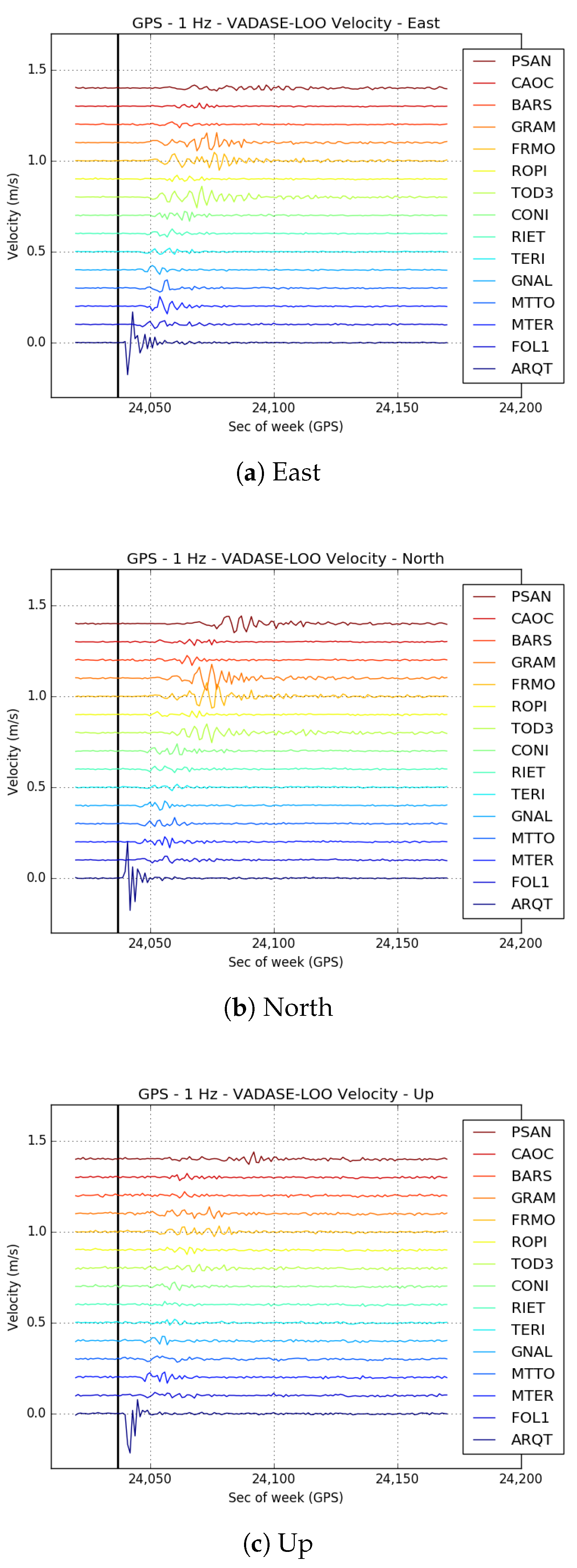
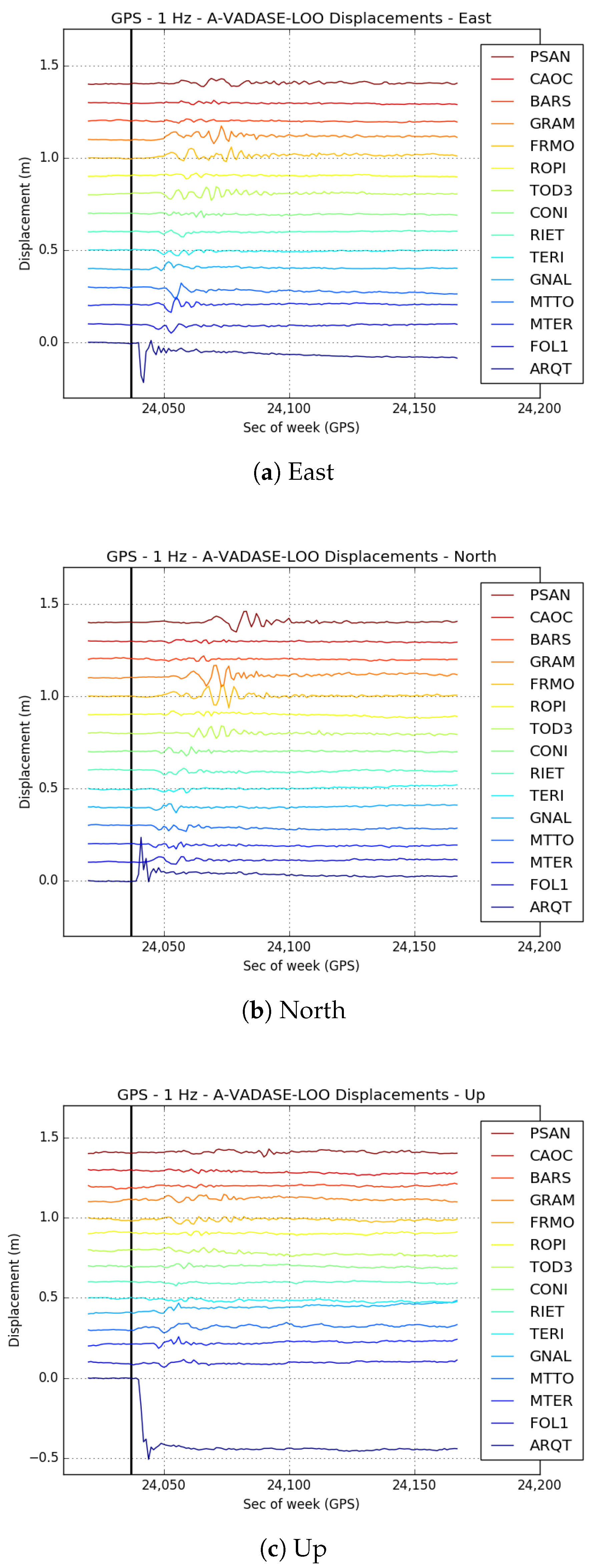
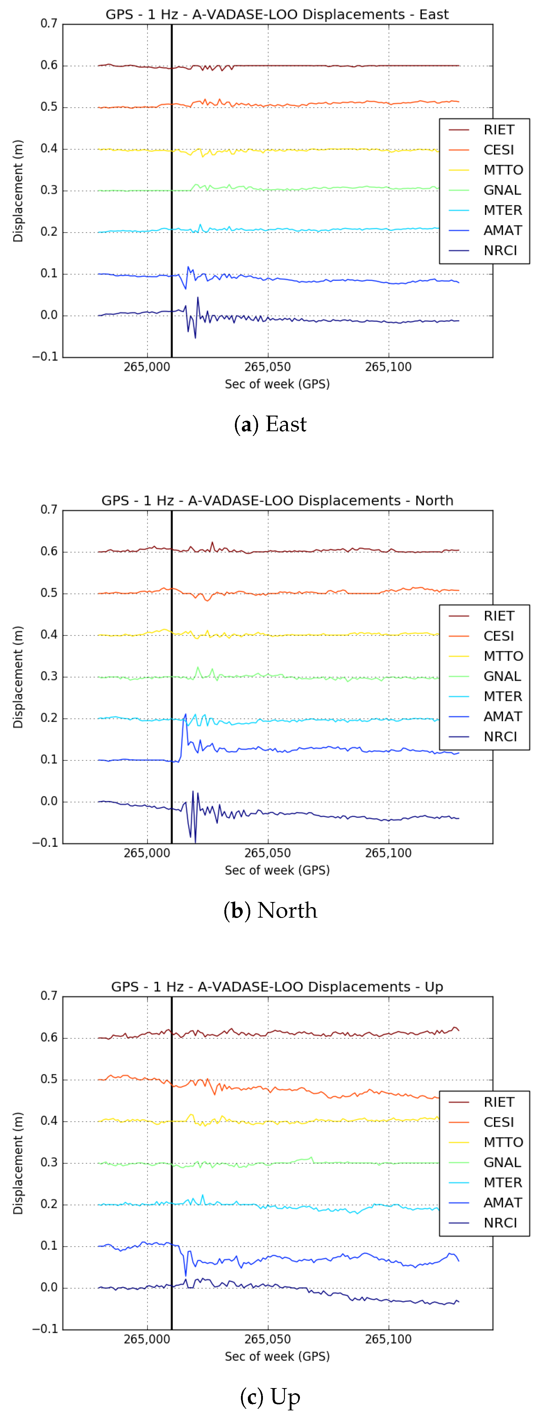
The observations data were processed with the VADASE improved algorithm (VADASE-LOO and A-VADASE), estimating the 3D velocities (east, north and up components); for the 30 October earthquake, these velocities are displayed in
Figure 2 for the 150-s interval across the mainshock, when the earthquake signatures were clearly evident. In
Figure 2,
Figure 3,
Figure 4,
Figure 5 and
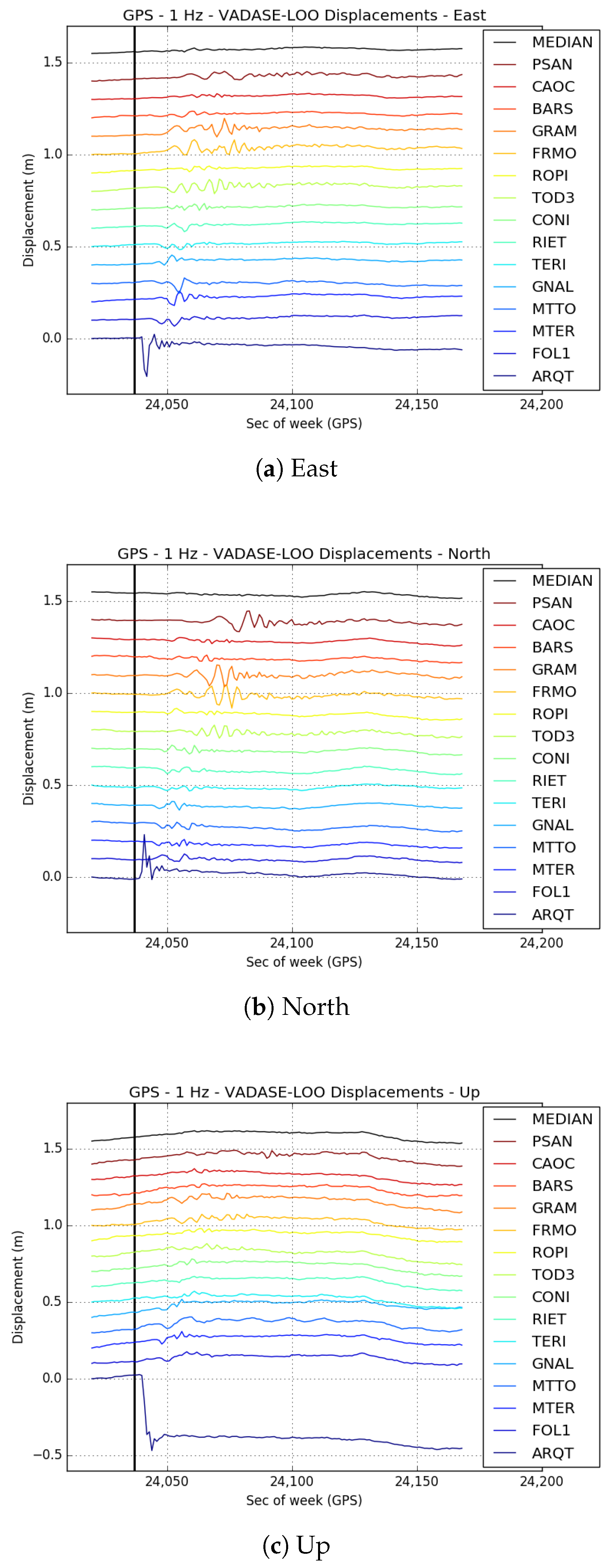
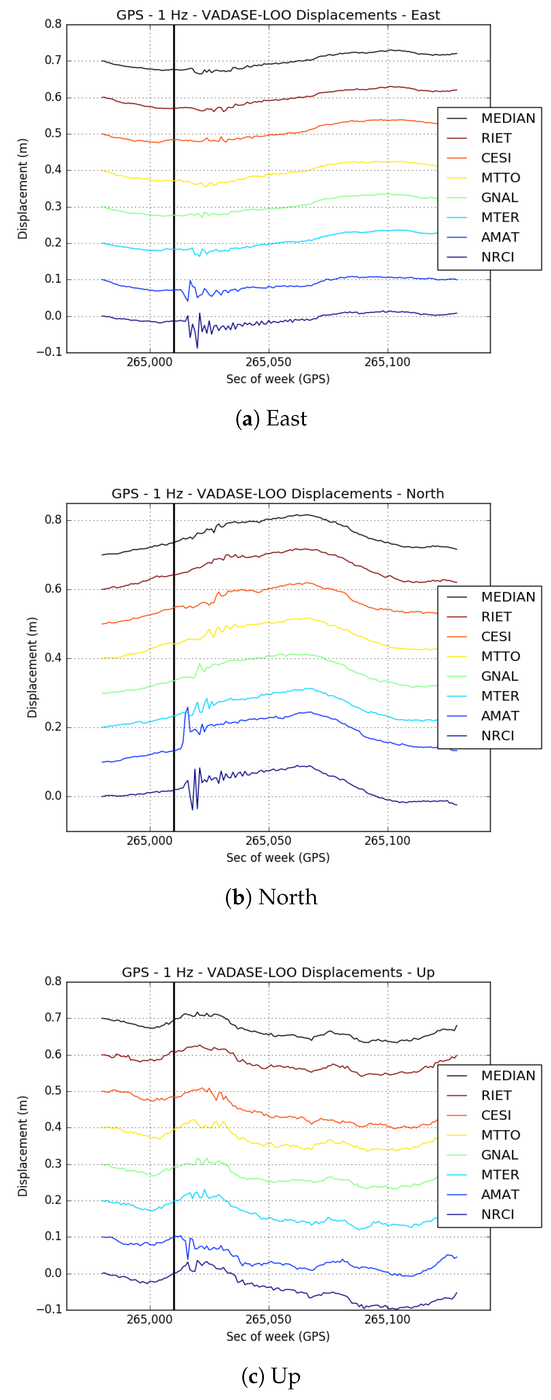
Figure 6, the velocities, the displacements and the detrended displacements are represented, ordering the stations from the bottom to the top in dependence of their distance from the epicenter (the nearest station in the bottom and the farthest on the top) and shifting the velocities, the displacements and the detrended displacements by 0.1 mm/s, 0.1 mm each.
In order to depict the waveforms and to quantify the coseismic displacements, the 3D velocities were integrated. This integration is very sensitive to estimation biases, mainly due to residual clock and orbit errors, which accumulate over time and display their signature as a trend in the coseismic displacements. Examples of these trends for the 30 October earthquake and the 24 August earthquake are respectively shown in
Figure 3 and, more evidently, in
Figure 4.
A-VADASE strategy was applied to remove the spatial correlated trends; the detrended coseismic displacements, called A-VADASE-LOO, are displayed in
Figure 5 and
Figure 6.
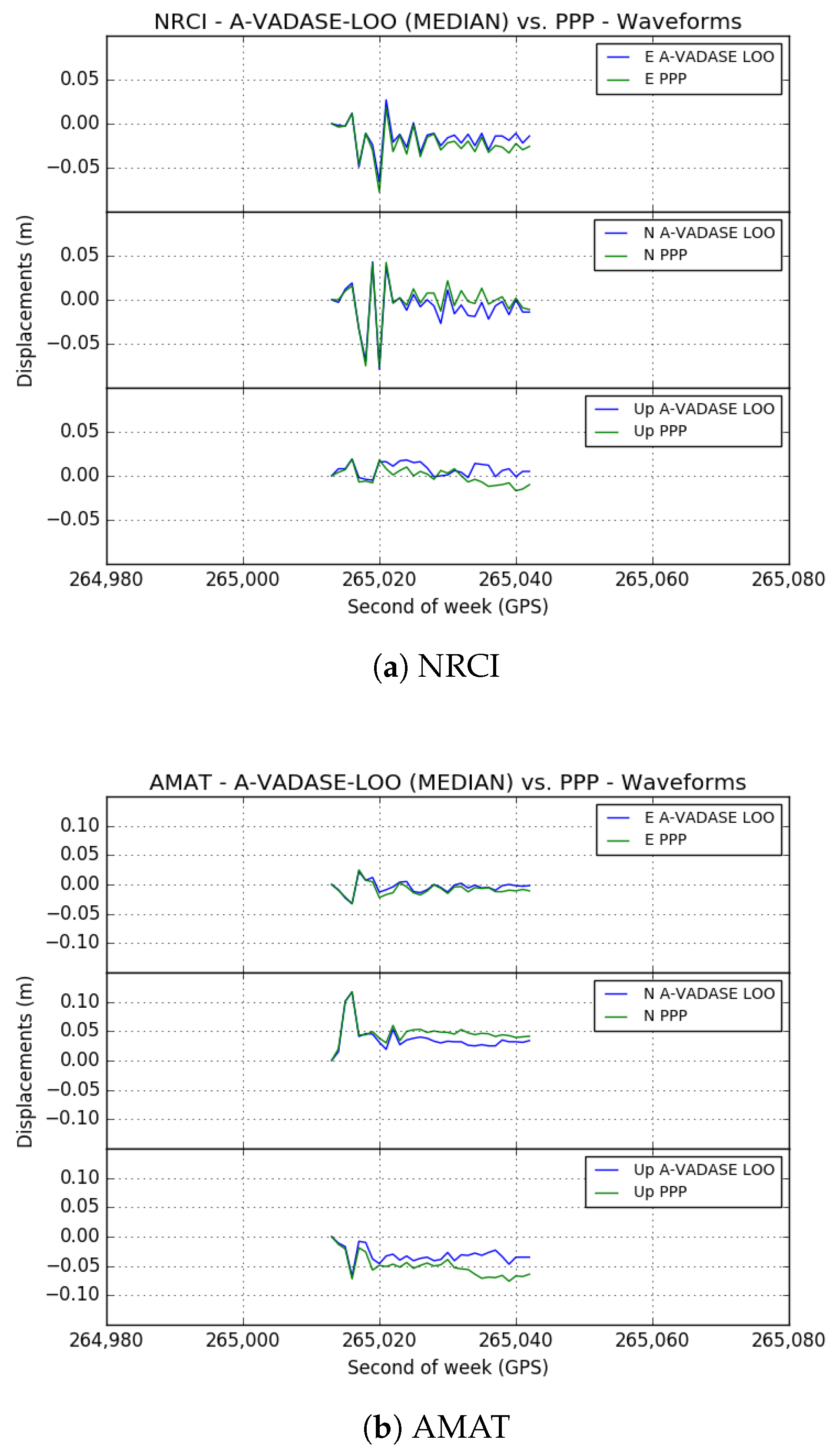
A-VADASE-LOO solutions were compared to the results obtained, with the same dataset, using Point Positioning Processing (PPP) strategy. The Kinematic PPP is free and online through a well-known and reliable online service, Automatic Precise Positioning Service (APPS), which applies the most advanced GPS positioning technology from NASA’s Jet Propulsion Laboratory (JPL) to estimate the position of GPS receivers (
http://apps.gdgps.net/). The observation files provided to the PPP services are relative to two hours: one hour before and one hour after the earthquake main shock beginning at the nearest station.
For each station, the two solutions (A-VADASE-LOO vs PPP) were aligned (i.e., their difference was set to zero) at a conventional initial epoch (starting epoch of the station nearest to the epicenter) and compared within a time interval of ten seconds, corresponding to the significant shaking duration detected by GNSS. The retrieved positions were differenced at the corresponding epochs, and the agreement between the solutions was evaluated by the RMSE of the differences. For the sake of brevity, only the graphic results related to the two GNSS stations nearest the epicenter are presented for the 24 August and 30 October earthquakes (
Figure 7 and
Figure 8); on the other hand, the tables of the differences for all the GNSS stations and for all the earthquakes are presented (
Table 2,
Table 3 and
Table 4).
The comparisons between A-VADASE-LOO and PPP for all components (east, north and up) and for all earthquakes demonstrated the reliability and the high accuracy of the VADASE solutions; the differences between the two approaches, in terms of RMSE on the three components, were (in the average) in the order of 0.5–1 cm in the horizontal components east-north and in the order of 1–1.5 cm in height (
Table 2,
Table 3 and
Table 4).
3. VADASE Real-Time Coseismic Displacements
It is well known that the knowledge of the coseismic displacements field is the key information for seismic inversion and the studies about the fault source mechanism. Whereas, the off-line estimation of the coseismic displacement field has been repeatedly proven successful on the basis of InSAR and GNSS dense networks (some relevant examples are described in [
15,
16,
17] and in [
18,
19,
20]), this estimation in real time can only be based on GNSS permanent networks, and it is still a challenge at the international level, where the problem is faced with the primary goal of supplying timely information for tsunami early warning [
21]. This is the why, here, a new real-time strategy to coseismic displacement estimation based on the VADASE solution is proposed. The results coming from this strategy are compared to a second solution obtained by the PPP technique and to the standard off-line (also called static) solution.
3.1. VADASE Solution
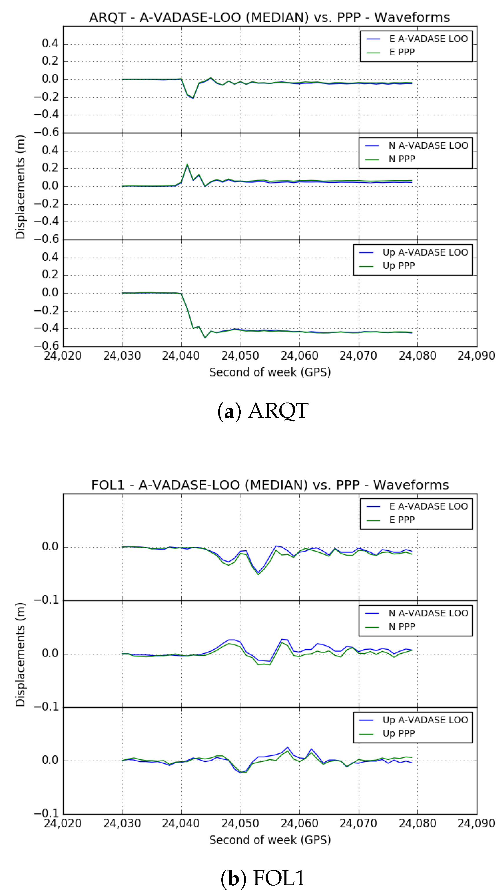
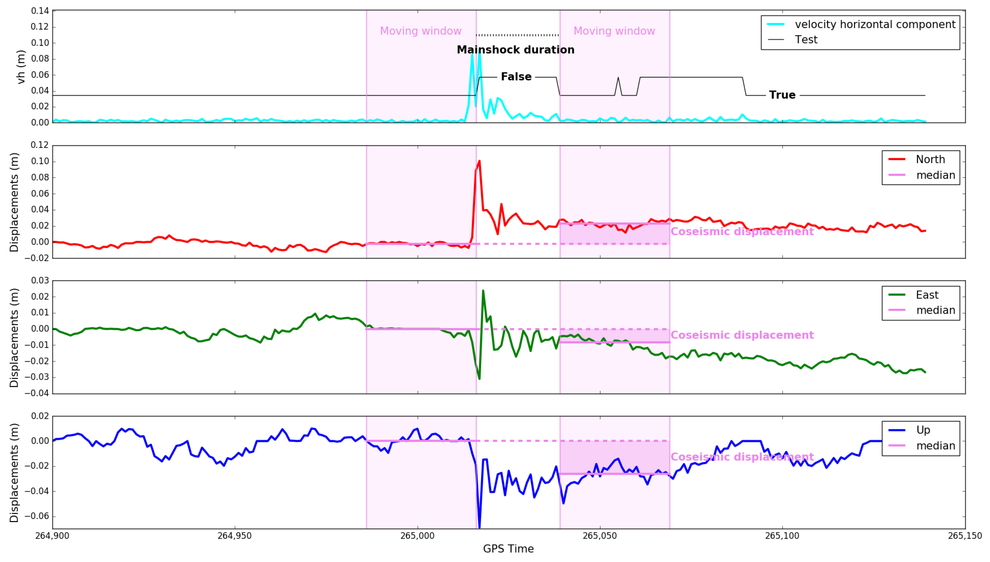
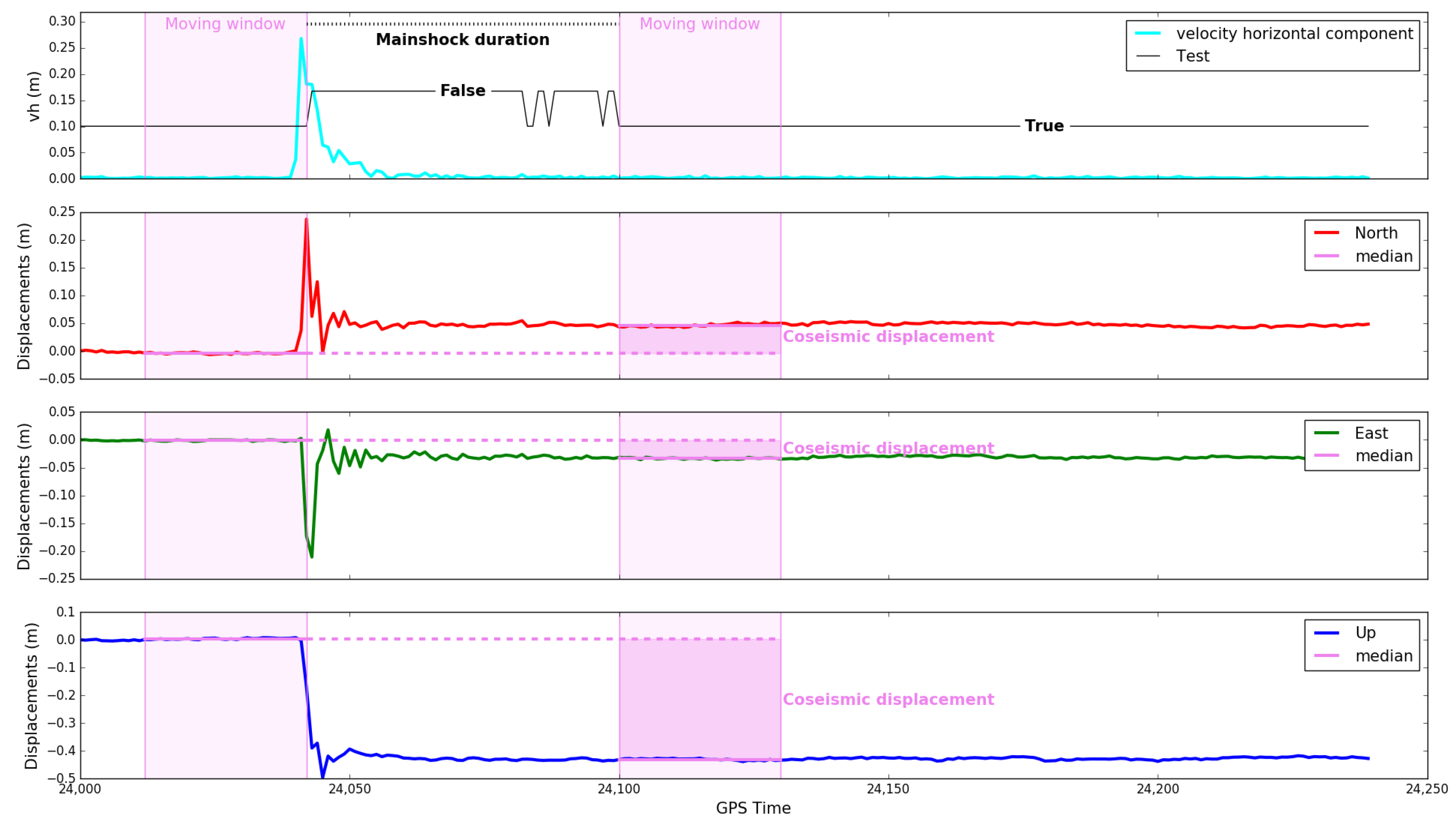
The main idea underlying VADASE real-time coseismic displacement estimation is to define the significant shaking duration detectable by GNSS on the basis of the mean noise level of the VADASE velocity solution, which has been recognized to be constant with a Gaussian distribution before and after the earthquake shaking, and to estimate the displacement occurring across the shaking interval.
In detail, at first, on the basis of a chosen time moving window (here, e.g., 30 s long), it is possible to compute the mean noise level (standard deviation) of the horizontal velocity component just before the beginning of the earthquake shaking, that is in an undisturbed situation (reference standard deviation
); only the horizontal velocity component is considered, since it is less noisy with respect to the 3D velocity and therefore more sensitive to the shaking. Then, moving this window epoch-by-epoch, the standard deviation (at epoch
i,
) of the horizontal velocity is computed across the earthquake shaking, which leads to an increase of the standard deviation itself. The running standard deviation at each epoch
is tested against the reference standard deviation
, in order to detect when they again become equal from the statistical point of view, so that significant shaking is over; to this aim, the standard statistical test for variance comparison for independent samples of equal size is used, under the hypothesis (generally well confirmed) that the noise of the horizontal velocity component is Gaussian in an undisturbed situation:
where
N is the size (here 30, with a sampling rate of 1 s) of both samples. Note that the latency to define the starting and ending epochs of the significant shaking is at least equal to the length of the moving window. Moreover, to make the real-time coseismic displacement estimation procedure more reliable avoiding the solution being dependent on the spurious oscillation of the
statistic, it was decided to define the starting epoch of the significant shaking only when
exceeded the threshold of the Fisher value at a certain significance level (here chosen equal to 1%) for at least five consecutive epochs at an observation rate of 1 Hz and, correspondingly, the end epoch only when
was below the same threshold again for at least five consecutive epochs. Note that in the case that the observation rate is higher, the number of consecutive epochs to be considered to define the starting and the ending epochs must proportionally increase.
After having determined the duration of the significant shaking, the coseismic displacement was estimated as the difference between the medians of the displacements within the moving windows respectively corresponding to the ending and the starting epochs (e.g., in
Figure 9 and
Figure 10).
3.2. PPP Solution
The same strategy defined to estimate coseismic displacements on the basis of VADASE solutions was applied to the solutions derived through PPP by using Automatic Precise Positioning Server PPP online tools, based on GIPSY 6.4 (APP-PPP,
http://apps.gdgps.net/). However, in this case, a much longer data interval (in our case, 2 h before the earthquake plus 150 s) was necessary with respect to the few minutes used for the VADASE solution, in order to guarantee the fixing of the initial ambiguities [
22]. We acknowledge that, in principle, this is not a severe drawback, provided continuous data are collected, as it is standard if a GNSS permanent network is available. Note that PPP (here used in post-processing) is also able to estimate real-time solutions, provided precise orbit and clock products are available in real time, as well, as those supplied by the International GNSS Service Real-Time Service (
http://www.igs.org/rts) or other similar services.
3.3. INGV Static Solution
The coseismic displacements were obtained from the GPS data acquired by the very large GNSS network (more than 1000 permanent stations, mostly at a 30-s sampling rate, only few at 1 s) routinely processed daily at the Istituto Nazionale di Geofisica e Vulcanologia (INGV) [
23,
24]. The available GPS data, in the form of 24-h 30-s sampling rate RINEX files, were processed by three different analysis groups, using different software (BERNESE,
http://www.bernese.unibe.ch; GAMIT,
http://www.gpsg.mit.edu/~simon/gtgk; and GIPSY,
http://gipsy.jpl.nasa.gov/orms/goa). The three processing approaches are well described in [
12], usually devoted to estimating velocity and strain rate fields. The static coseismic displacements are computed from three distinct time series of stations located around the epicenters from the linear model:
where
are the Cartesian coordinates at epoch
t of each site (
i = 1, 2, 3),
are the coordinates at reference epoch
,
are the rates,
and
are the amplitude and phase of periodical signals (mostly annual) and
H is the Heaviside step function, used to estimate the coordinate offsets (
) at a given epoch
.
The three sets of independent coseismic displacements were estimated by excluding the Day of the Earthquake (DOE) and limiting the time series to the 15 days before DOE and only to the three days after DOE, to minimize the effects of early postseismic displacements, commonly observed in a wide range of seismic events causing deformations up to several centimeters, depending on the magnitude and the driving mechanism. The three independent coseismic displacements estimates were then combined to obtain a final field of validated displacements, following the procedure described in [
25] and first applied in [
26]. The combination allows one to obtain a final revised solution, with efficient outlier detection obtained after cross-checking independent solutions and realistic estimates of the displacement uncertainties.
3.4. Results
The coseismic displacements estimated in a real-time scenario (that is in post-processing in a retrospective analysis, but using only the information that would have been available in real time) from A-VADASE-LOO and in post-processing from PPP using the described original procedure, as well as from routine INGV daily solution are reported in
Table 5,
Table 6 and
Table 7. Note that the combined INGV coseismic displacements after the 24 August, 26 October and 30 October 2016 earthquakes (INGV Working Group “GPS Geodesy (GPS data and data analysis center)”, 2016) are fully available at
http://ring.gm.ingv.it [
27,
28,
29].
The differences between the estimated coseismic displacements according to the three different approaches (VADASE, PPP, static) and the main statistical indices of these differences (mean, Standard Deviation (St.Dev.) and Root Mean Square Error (RMSE)) are summarized in
Table 8,
Table 9 and
Table 10.
It is important to highlight that the agreement between the two potentially real-time solutions (VADASE and PPP) was at a level better than 1 cm for the horizontal components and around 2 cm in height, which would not be satisfying for small coseismic displacements, but it is certainly appropriate for larger displacements, as for ARQT station in the 30 October 2016 earthquake, where the agreement was even better. Moreover, the agreement of the VADASE real-time scenario solution with the INGV static solution is better than for the PPP solution, at a level of 0.5–1 cm in the horizontal components and of 1–1.5 cm in height.
4. Conclusions and Prospects
VADASE (Variometric Approach for Displacement Analysis Standalone Engine) is an approach to estimate in real-time the 3D displacements of a single GNSS receiver, just using the time differences of the high-rate (i.e., 1 Hz or more) carrier phase observations, together with the broadcast orbits and clocks.
This paper proposed two improvements to overcome two well-known problems of the VADASE solution, that is spurious oscillations in the velocity estimates due to outliers in GNSS observations and trends in the derived displacements due to errors in broadcast orbits and clocks. With regard to the first problem, a strategy (VADASE-LOO) to detect outliers in the observations during the real-time estimation was defined, on the basis of the Leave-One-Out Cross-Validation (LOOCV). With regards to the second problem, at first, a strong spatial correlation of these trends among close GNSS stations was clearly identified, so that an augmentation strategy (A-VADASE) was introduced to filter out them on the basis of a spatial median.
The two new strategies were applied to data collected during the recent three strong earthquakes that occurred in Central Italy on 24 August, 26 and 30 October 2016, and it was demonstrated that the combination of VADASE-LOO and A-VADASE has a positive impact, leading to the enhanced A-VADASE-LOO solution. The comparison with the well-known PPP solution, here computed in post-processing using the best available products (IGS final orbits and clocks), showed an agreement between the two approaches in terms of RMSE at a level of 0.5–1 cm in the horizontal components east-north and at the level of 1–1.5 cm in height.
Moreover, an original strategy for real-time estimation of coseismic displacements, based on the A-VADASE-LOO solution, was also introduced, based on the well-confirmed hypothesis of constant and Gaussian noise of the VADASE solution just before and after a ground shaking event due to an earthquake.
Again, this original strategy was applied to the same above-mentioned data, and a quite good agreement was shown, both with the INGV static solutions, at a level of 0.5–1 cm in the horizontal components and of 1–1.5 cm in height, and with the PPP post-processed solutions, at a level better than 1 cm for the horizontal components and around 2 cm in height. These levels of agreement, quite similar to those between the INGV static and the PPP post-processed solutions, confirmed that the proposed real-time strategy was able to provide coseismic displacements at state-of-the-art accuracy, and this is compliant with the goals of the GNSS Augmentation for Tsunami Early Warning (GATEW) initiative promoted by the Global Geodetic Observing System (GGOS) Geohazard Focus Area.
As regards future prospects, three main issues have to be considered: at first, A-VADASE-LOO solution needs to undergo further assessments, applying and comparing it both to the standard VADASE solution and to other independent solutions; moreover, further checks are needed in order to define the proper length of the moving windows in order to keep the latency as short as possible; finally, the real-time coseismic estimation procedure has to be additionally checked also in the case of higher observation rates, in order to better assess the criteria to select the minimum number of consecutive epochs to define the starting and the ending of the significant shaking epoch.
Author Contributions
Conceptualization, M.C., A.M. Methodology, M.C. Software, F.F., G.S., A.M. Formal analysis, F.F., G.S., M.C.D., F.R., R.D., G.P. Investigation, F.F., G.S., M.C.D., F.R., R.D., G.P. Writing, original draft preparation, F.F., M.C.D. Writing, Review and editing, F.F., G.S., A.M., M.C., F.R., R.D., G.P. Visualization, F.F. Supervision, M.C. Funding acquisition, M.C.
Funding
This research was partially supported by the University of Rome “La Sapienza”, through a PhD fellowship granted to Giorgio Savastano.
Acknowledgments
We wish to thank all the agencies involved in GNSS network development and maintenance: INGV (RING WG
http://ring.gm.ingv.it), ISPRA—Istituto Superiore per la Protezione e la Ricerca Ambientale (
http://www.isprambiente.gov.it), DPC—Dipartimento Protezione Civile (
http://www.protezionecivile.gov.it), Regione Lazio (
http://gnss-regionelazio.dyndns.org), Regione Abruzzo (
http://gnssnet.regione.abruzzo.it), SmartNet ITALPOS (
http://it.smartnet-eu.com) and NetGEO (
http://www.netgeo.it). VADASE is the subject of an international pending patent, generously supported by the University of Rome “La Sapienza” and by its Start-Up Kuaterion srl. VADASE was awarded the DLR (German Aerospace Agency) Special Topic Prize and the Audience Award at the European Satellite Navigation Competition 2010. It was partially developed thanks to a one-year cooperation with the DLR Institute for Communications and Navigation at Oberpfaffenhofen (Germany) and was included in the Success Stories of the European Satellite Navigation Competition 2012.
Conflicts of Interest
The authors declare no conflict of interest.
Abbreviations
The following abbreviations are used in this manuscript:
| CDDIS | Crustal Dynamics Data Information System |
| EOP | Earth Orientation Parameters |
| GGOS | Global Geodetic Observing System |
| GNSS | Global Navigation Satellite System |
| GPS | Global Positioning System |
| HR | High Rate |
| INGV | Istituto Nazionale di Geofisica e Vulcanologia |
| ITRF | International Terrestrial Reference Frame |
| LOOCV | Leave-One-Out Cross-Validation |
| PPP | Precise Point Positioning |
| RINEX | Receiver Independent Exchange Format |
| RING | Rete Integrata Nazionale GPS |
| RMSE | Root Mean Square Error |
| UTC | Universal Time Coordinated |
| VADASE | Variometric Approach for Displacement Analysis Stand-alone Engine |
Appendix A
Here, some technical details are given on the application of the Leave-One-Out (LOO) strategy to the VADASE algorithm for the identification and removal of possible outliers in the phase observations; for additional information about LOO, please refer to [
3,
5].
If n satellites common to two consecutive epochs are available, so that n variometric equations can be written, the LOO method requires n different least squares solutions for these consecutive epochs, each of them based on variometric equations leaving out one satellite, different in each solution.
Therefore, to decide if the observations vector
includes an outlier, that means that one observation does not follow the standard (linearized) functional model:
where
y is the observables vector (
n, in our case),
A is the design matrix,
x is the vector of the parameters (just four for each couple of epochs in the VADASE solution) and
b is the known term; one observation is removed at each time. The functional model (
A1) is rewritten as follows:
where
is the last observable,
R is the last row of the matrix
A and
is the last known term; without losing generality, since the equations can change their order in
A1, the possible outlier is supposed to impact just the last equation, so that the corresponding observation
has to be checked and is excluded from the estimation process.
If only the first
observations are used to estimate the parameters
x, the
vector is obtained, which is not affected by the possible outlier:
where
is the weight matrix without the last row and column.
Under the hypothesis of the Gaussian observations, for the excluded n-th observation, the statistical
is computed, defined as:
where the subscript
n refer to the excluded observation and where:
On the other hand, the
is:
where:
where
is the weight of the excluded observation.
Since the
is unknown, the estimated
is used in (
A7):
and:
Under the hypothesis that the excluded observation does not contain any outlier, the index follows the t-Student distribution (), where are the degrees of freedom, in this case equal to ). Therefore, choosing a significance level (1% or 5%), the threshold to accept or reject is determined, so that it is possible to conclude that the excluded observation does not contain an outlier if is within the range .
References
- Colosimo, G.; Crespi, M.; Mazzoni, A. Real-time GPS seismology with a stand-alone receiver: A preliminary feasibility demonstration. J. Geophys. Res. 2011, 116, B11302. [Google Scholar] [CrossRef]
- Branzanti, M.; Colosimo, G.; Crespi, M.; Mazzoni, A. GPS Near-Real-Time Coseismic Displacements for the Great Tohoku-oki Earthquake. IEEE Geosci. Remote Sens. Lett. 2013, 10, 372–376. [Google Scholar] [CrossRef]
- Brovelli, M.A.; Crespi, M.; Fratarcangeli, F.; Giannone, F.; Realini, E. Accuracy assessment of high resolution satellite imagery orientation by leave-one-out method. ISPRS J. Photogramm. Remote Sens. 2008, 63, 427–440. [Google Scholar] [CrossRef]
- Fratarcangeli, F.; Ravanelli, M.; Mazzoni, A.; Colosimo, G.; Benedetti, E.; Branzanti, M.; Savastano, G.; Verkhoglyadova, O.; Komjathy, A.; Crespi, M. The variometric approach to real-time high-frequency geodesy. Rendiconti Lincei. Scienze Fisiche e Naturali 2018, 29 (Suppl. 1), S95–S108. [Google Scholar] [CrossRef]
- Biagi, L.; Caldera, S. An efficient Leave One Block Out approach to identify outliers. J. Appl. Geod. 2013, 7, 11–19. [Google Scholar] [CrossRef]
- Baarda, W. A testing procedure for use in geodetic networks. In Publ Geod 2(5); Netherlands Geodetic Commission: Delft, The Netherlands, 1968; ISBN-13 978 90 6132 209 2, ISBN-10 90 6132 209. [Google Scholar]
- Li, X.; Ge, M.; Guo, B.; Wickert, J.; Schuh, H. Temporal point positioning approach for real-time GNSS seismology using a single receiver. Geophys. Res. Lett. 2013, 40, 5677–5682. [Google Scholar] [CrossRef] [Green Version]
- Hung, H.K.; Rau, R.J.; Benedetti, E.; Branzanti, M.; Mazzoni, A.; Colosimo, G.; Crespi, M. GPS Seismology for a moderate magnitude earthquake: Lessons learned from the analysis of the 31 October 2013 ML 6.4 Ruisui (Taiwan) earthquake. Ann. Geophys. 2017, 60, S0553. [Google Scholar] [CrossRef]
- Wdowinski, S.; Bock, Y.; Zhang, J.; Fang, P.; Genrich, J. Southern California permanent GPS geodetic array: Spatial filtering of daily positions for estimating coseismic and postseismic displacements induced by the 1992 Landers earthquake. J. Geophys. Res. 1997, 102, 18057–18070. [Google Scholar] [CrossRef] [Green Version]
- Devoti, R.; Riguzzi, F.; Cuffaro, M.; Doglioni, C. New GPS constraints on the kinematics of the Apennines subduction. Earth Planet. Sci. Lett. 2008, 273, 163–174. [Google Scholar] [CrossRef]
- Locati, M.; CAMASSI, R.D.; Rovida, A.N.; Ercolani, E.; BERNARDINI, F.M.A.; Castelli, V.; Caracciolo, C.H.; Tertulliani, A.; Rossi, A.; Azzaro, R.; et al. DBMI15, the 2015 version of the Italian Macroseismic Database. Istituto Nazionale di Geofisica e Vulcanologia 2016. [Google Scholar] [CrossRef]
- Devoti, R.; D’Agostino, N.; Serpelloni, E.; Pietrantonio, G.; Riguzzi, F.; Avallone, A.; Cavaliere, A.; Cheloni, D.; Cecere, G.; D’Ambrosio, C.; et al. The Mediterranean Crustal Motion Map compiled at INGV. Ann. Geophys. 2017, 60. [Google Scholar] [CrossRef]
- Falcucci, E.; Gori, S.; Galadini, F.; Fubelli, G.; Moro, M.; Saroli, M. Active faults in the epicentral and mesoseismal Ml 6.0 24, 2016 Amatrice earthquake region, Central Italy. Methodological and seismotectonic issues. Ann. Geophys. 2016, 59. [Google Scholar] [CrossRef]
- Altamimi, Z.; Métivier, L.; Collilieux, X. ITRF2008 plate motion model. J. Geophys. Res. 2012, 117, B07402. [Google Scholar] [CrossRef]
- Atzori, S.; Hunstad, I.; Chini, M.; Salvi, S.; Tolomei, C.; Bignami, C.; Stramondo, S.; Trasatti, E.; Antonioli, A.; Boschi, E. Finite fault inversion of DInSAR coseismic displacement of the 2009 L’Aquila earthquake (Central Italy). Transl. World Seismol. 2009, 36, L15305. [Google Scholar]
- Funning, G.J.; Parsons, B.; Wright, T.J.; Jackson, J.A.; Fielding, E.J. Surface displacements and source parameters of the 2003 Bam (Iran) earthquake from Envisat advanced synthetic aperture radar imagery. J. Geophys. Res. 2005, 110, B09406. [Google Scholar] [CrossRef]
- Wright, T.J.; Lu, Z.; Wicks, C. Source model for the Mw 6.7, 23 October 2002, Nenana Mountain earthquake (Alaska) from InSAR. Geophys. Res. Lett. 2003, 30, 1974. [Google Scholar] [CrossRef]
- Langbein, J.; Bock, Y. High-rate real-time GPS network at parkfield: Utility for detecting fault slip and seismic displacements. Geophys. Res. Lett. 2004, 31. [Google Scholar] [CrossRef]
- Larson, K. GPS seismology. J. Geod. 2009, 83, 227–233. [Google Scholar] [CrossRef]
- Ohta, Y.; Kobayashi, T.; Tsushima, H.; Miura, S.; Hino, R.; Takasu, T.; Fujimoto, H.; Iinuma, T.; Tachibana, K.; Demachi, T.; et al. Quasi real-time fault model estimation for near-field tsunami forecasting based on RTK-GPS analysis: Application to the 2011 Tohokuoki earthquake (Mw 9.0). J. Geophys. Res. 2012, 117, B02311. [Google Scholar] [CrossRef]
- GATEW Working Group. Report of the GNSS Tsunami Early Warning System Workshop, 25–27 July 2017, Sendai, Japan. GGOS Focus Area Geohazard. 2018. Available online: https://apru.org/partnering-on-solutions/multi-hazards-program/item/939-2017-gnss-tsunami-early-warning-system-workshop (accessed on 29 July 2018).
- Benedetti, E.; Branzanti, M.; Biagi, L.; Colosimo, G.; Mazzoni, A.; Crespi, M. Global Navigation Satellite Systems Seismology for the 2012 Mw 6.1 Emilia Earthquake: Exploiting the VADASE Algorithm. Seismol. Res. Lett. 2014, 85, 649–656. [Google Scholar] [CrossRef]
- Devoti, R.; Pietrantonio, G.; Riguzzi, F. GNSS networks for Geodynamics in Italy. Fisica de la Tierra 2012, 26, 11–24. [Google Scholar] [CrossRef]
- Devoti, R.; Riguzzi, F. The velocity field of the Italian area. Rend. Fis. Acc. Lincei 2018, 29 (Suppl. 1), 51–58. [Google Scholar] [CrossRef]
- Devoti, R. Combination of coseismic displacement field: A geodetic perspective. Ann. Geophys. 2012, 55. [Google Scholar] [CrossRef]
- Serpelloni, E.; Anderlini, L.; Avallone, A.; Cannelli, V.; Cavaliere, A.; Cheloni, D.; D’Ambrosio, C.; D’Anastasio, E.; Esposito, A.; Pietrantonio, G.; et al. GPS observations of coseismic deformation following the May 20 and 29, 2012, Emilia seismic events (northern Italy): data, analysis and preliminary models. Ann. Geophys. 2012, 55. [Google Scholar] [CrossRef]
- Ring Group. High-Rate GPS Data Archive of the 2016 Central Italy Seismic Sequence; INGV: Roma, Italy, 2017. [Google Scholar] [CrossRef]
- Ring Group. Preliminary Co-Seismic Displacements for the October 26 (Mw 5.9) and October 30 (Mw 6.5) Central Italy Earthquakes from the Analysis of GPS Stations; INGV: Roma, Italy, 2017. [Google Scholar] [CrossRef]
- Ring Group. Co-Seismic Displacements for the 24 August 2016 Ml6, Amatrice (Central Italy) Earthquake Estimated From Continuous GPS Stations; INGV: Roma, Italy, 2017. [Google Scholar] [CrossRef]
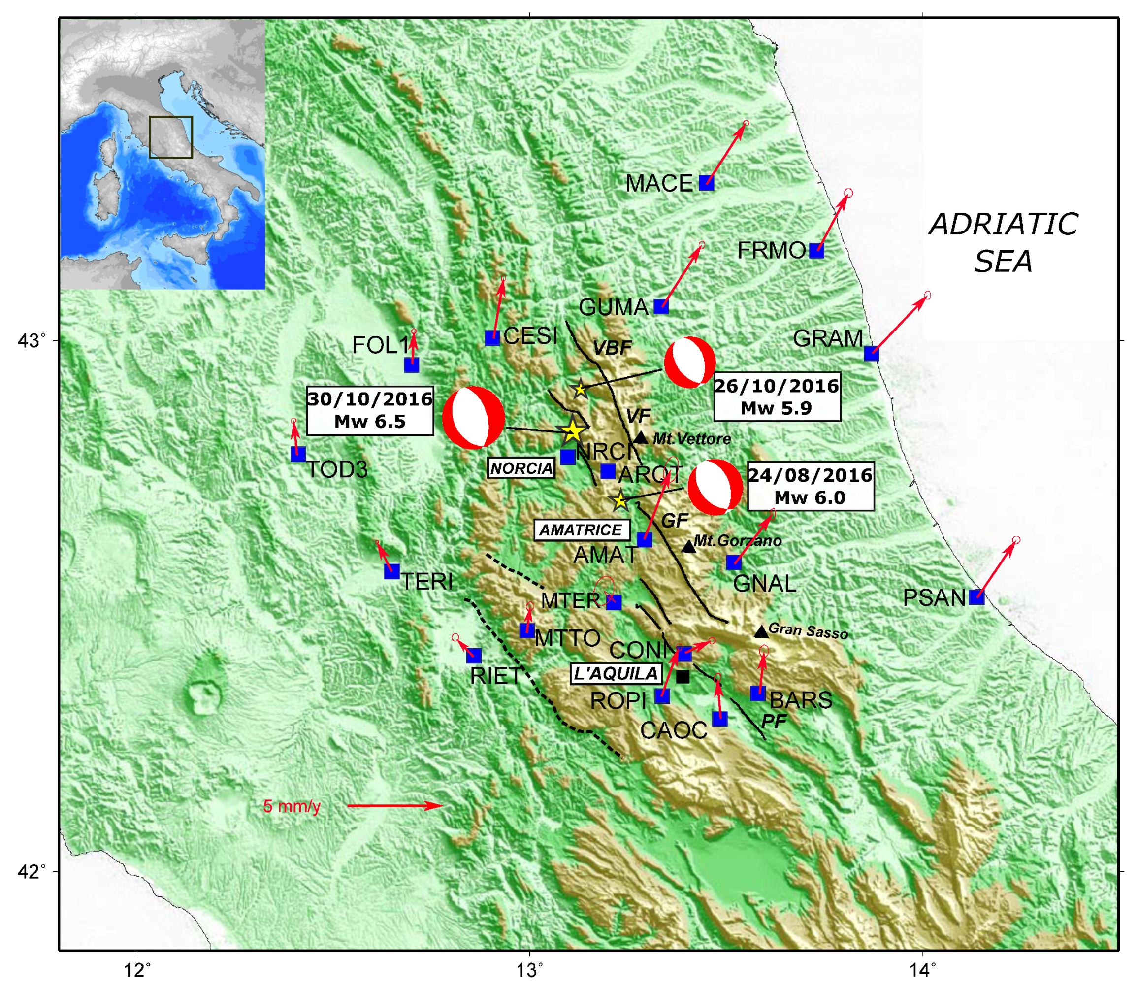
Figure 1.
GPS sites (blue squares); GPS velocities in the Eurasian fixed reference frame from [
12] (red arrows); main faults from [
13] (black lines: VBF: Vettore-Bove Fault; VF: Vettore Fault; GF: Gorzano Fault; PF: Paganica Fault); focal mechanisms of the three events show the extensional style (red and white beach balls). Velocities with respect to the Eurasian fixed frame [
14] and error ellipses at the one sigma confidence level are shown.
Figure 2.
Estimated velocity by VADASE-LOO for the 150-s interval across the 30 October 2016 main shock (GPS time).
Figure 2.
Estimated velocity by VADASE-LOO for the 150-s interval across the 30 October 2016 main shock (GPS time).
Figure 3.
Estimated displacements by VADASE-LOO for the 150-s interval across the 30 October 2016 main shock (GPS time).
Figure 3.
Estimated displacements by VADASE-LOO for the 150-s interval across the 30 October 2016 main shock (GPS time).
Figure 4.
Estimated displacements by VADASE-LOO for the 150-s interval across the 24 August 2016 main shock (GPS time).
Figure 4.
Estimated displacements by VADASE-LOO for the 150-s interval across the 24 August 2016 main shock (GPS time).
Figure 5.
Estimated displacements after detrending by A-VADASE-LOO for the 150-s interval across the 30 October 2016 main shock (GPS time).
Figure 5.
Estimated displacements after detrending by A-VADASE-LOO for the 150-s interval across the 30 October 2016 main shock (GPS time).
Figure 6.
Estimated displacements after detrending by A-VADASE-LOO for the 150-s interval across the 24 August 2016 main shock (GPS time).
Figure 6.
Estimated displacements after detrending by A-VADASE-LOO for the 150-s interval across the 24 August 2016 main shock (GPS time).
Figure 7.
A-VADASE-LOO vs. PPP in the 30-s interval across the 24 August 2016 main shock (GPS time).
Figure 7.
A-VADASE-LOO vs. PPP in the 30-s interval across the 24 August 2016 main shock (GPS time).
Figure 8.
A-VADASE-LOO vs. PPP in the 30-s interval across the 30 October 2016 main shock (GPS time).
Figure 8.
A-VADASE-LOO vs. PPP in the 30-s interval across the 30 October 2016 main shock (GPS time).
Figure 9.
VADASE real-time coseismic displacement estimation at AMAT (Amatrice) for the 24 August 2016 main shock.
Figure 9.
VADASE real-time coseismic displacement estimation at AMAT (Amatrice) for the 24 August 2016 main shock.
Figure 10.
VADASE real-time coseismic displacement estimation at ARQT (Arquata del Tronto) for the 30 October 2016 main shock.
Figure 10.
VADASE real-time coseismic displacement estimation at ARQT (Arquata del Tronto) for the 30 October 2016 main shock.
Table 1.
Number of outliers in the 3D velocity variometric solutions over 67 days (3 February–9 April 2016) at the M0SE IGS permanent station.
Table 1.
Number of outliers in the 3D velocity variometric solutions over 67 days (3 February–9 April 2016) at the M0SE IGS permanent station.
| Type of Solution | Number of Outliers |
|---|
| East | North | Up |
|---|
| VADASE | 140 | 188 | 126 |
| VADASE-LOO | 12 | 48 | 33 |
Table 2.
Comparison between A-VADASE-LOO and PPP solutions: 24 August 2016 earthquake.
Table 2.
Comparison between A-VADASE-LOO and PPP solutions: 24 August 2016 earthquake.
| Station | RMSE (cm) |
|---|
| East | North | Up |
|---|
| NORC | 0.7 | 0.9 | 1.1 |
| AMAT | 0.6 | 1.3 | 2.3 |
| MTER | 0.7 | 1.4 | 1.4 |
| MTTO | 0.5 | 1.8 | 2.0 |
| CESI | 0.5 | 2.6 | 1.5 |
| GNAL | 0.4 | 0.7 | 0.3 |
| RIET | 0.5 | 0.6 | 0.9 |
Table 3.
Comparison between A-VADASE-LOO and PPP solutions: 26 October 2016 earthquake.
Table 3.
Comparison between A-VADASE-LOO and PPP solutions: 26 October 2016 earthquake.
| Station | RMSE (cm) |
|---|
| East | North | Up |
|---|
| GUMA | 0.5 | 1.5 | 1.2 |
| FOL1 | 1.3 | 0.6 | 1.1 |
| MACE | 0.4 | 0.5 | 1.2 |
| FRMO | 1.5 | 1.1 | 1.3 |
| TOD3 | 1.2 | 1.7 | 1.0 |
| GRAM | 1.0 | 0.8 | 1.7 |
| PSAN | 0.8 | 1.2 | 0.8 |
Table 4.
Comparison between A-VADASE-LOO and PPP solutions: 30 October 2016 earthquake.
Table 4.
Comparison between A-VADASE-LOO and PPP solutions: 30 October 2016 earthquake.
| Station | RMSE (cm) |
|---|
| East | North | Up |
|---|
| ARQT | 0.7 | 1.3 | 0.4 |
| FOL1 | 0.5 | 0.6 | 0.6 |
| MTER | 0.4 | 0.2 | 0.5 |
| MTTO | 0.5 | 0.2 | 1.2 |
| GNAL | 0.4 | 0.2 | 2.4 |
| TERI | 0.6 | 0.5 | 0.8 |
| RIET | 0.4 | 0.7 | 0.6 |
| CONI | 0.5 | 0.3 | 0.7 |
| TOD3 | 0.9 | 0.4 | 0.8 |
| FRMO | 0.5 | 0.3 | 0.5 |
| ROPI | 0.5 | 0.3 | 0.6 |
| GRAM | 0.9 | 0.7 | 1.9 |
| BARS2 | 0.5 | 0.5 | 1.0 |
| CAOC | 0.4 | 0.3 | 0.7 |
| PSAN | 0.4 | 0.3 | 1.4 |
Table 5.
Coseismic displacements: 24 August 2016 earthquake.
Table 5.
Coseismic displacements: 24 August 2016 earthquake.
| Station | INGV (cm) | PPP (cm) | A-VADASE-LOO (cm) |
|---|
| East | North | Up | East | North | Up | East | North | Up |
|---|
| AMAT | −1.1 | 2.2 | −1.5 | −0.5 | 2.5 | 4.5 | −0.8 | 2.5 | −2.6 |
| CESI | −0.0 | −0.2 | −0.2 | 0.6 | −0.8 | 2.2 | −0.0 | −0.4 | −1.2 |
| GNAL | 0.6 | 0.0 | −0.1 | − | − | − | 0.1 | 0.2 | 3.3 |
| MTER | −0.2 | −0.9 | 0.1 | −0.5 | 0.4 | −0.5 | 0.0 | −0.6 | 0.2 |
| MTTO | −0.3 | −0.5 | −0.2 | 0.1 | 0.5 | −0.7 | 0.1 | −0.3 | 0.3 |
| NRCI | −2.2 | −1.1 | 0.5 | −1.6 | −2.6 | 1.6 | −2.8 | −3.0 | −0.7 |
| RIET | −0.3 | −0.4 | 0.0 | −1.0 | −1.4 | −4.4 | 0.6 | −0.6 | 0.8 |
Table 6.
Coseismic displacements: 26 October 2016 earthquake.
Table 6.
Coseismic displacements: 26 October 2016 earthquake.
| Station | INGV (cm) | PPP (cm) | A-VADASE-LOO (cm) |
|---|
| East | North | Up | East | North | Up | East | North | Up |
|---|
| FOL1 | −0.5 | 0.2 | 0.3 | 0.3 | 0.1 | 1.2 | −0.1 | −0.5 | 0.0 |
| FRMO | 0.2 | 0.3 | −0.4 | −0.7 | 1.3 | −1.4 | −0.5 | 1.6 | −0.7 |
| GRAM | 0.1 | 0.1 | −0.2 | 1.0 | 1.6 | −0.1 | −0.5 | 0.1 | −0.6 |
| GUMA | 1.5 | 0.9 | −0.5 | 0.5 | −0.1 | 0.9 | 1.2 | 0.1 | −0.5 |
| MACE | 0.1 | 0.3 | −0.3 | −0.0 | 0.4 | 2.1 | −0.7 | 1.4 | 1.6 |
| PSAN | −0.1 | 0.1 | −0.2 | 0.6 | −0.2 | −2.3 | 1.0 | −0.8 | 0.5 |
| TOD3 | − | − | − | −0.5 | −0.8 | −1.5 | 1.3 | 0.7 | −2.1 |
Table 7.
Coseismic displacements: 30 October 2016 earthquake.
Table 7.
Coseismic displacements: 30 October 2016 earthquake.
| Station | INGV (cm) | PPP (cm) | A-VADASE-LOO (cm) |
|---|
| East | North | Up | East | North | Up | East | North | Up |
|---|
| ARQT | −4.4 | 5.3 | −44.7 | −3.9 | 5.6 | −43.4 | −3.2 | 5.0 | −43.4 |
| BARS | −0.0 | −0.0 | 0.8 | −0.1 | −0.5 | 0.8 | 0.2 | −0.4 | 1.0 |
| CAOC | 0.0 | −0.0 | 0.4 | 0.3 | −0.2 | 0.4 | 0.3 | −0.0 | −1.3 |
| CONI | 0.1 | −0.2 | 0.7 | 0.3 | −0.5 | 1.0 | −0.3 | 0.2 | 1.0 |
| FOL1 | −1.7 | 0.0 | −0.4 | −1.1 | 0.4 | 2.4 | 0.1 | 1.1 | 2.1 |
| FRMO | 0.8 | 0.7 | 0.7 | 1.1 | −0.2 | 5.4 | 1.5 | 0.1 | 0.7 |
| GNAL | 0.9 | −0.3 | 0.5 | 1.3 | −0.2 | 0.7 | 1.8 | −0.4 | 0.9 |
| GRAM | 1.2 | 0.4 | 0.4 | 0.5 | 0.1 | −2.5 | 1.9 | 2.2 | 0.9 |
| MTER | −0.1 | −1.0 | 0.3 | −0.0 | −1.1 | 0.6 | −0.0 | −1.0 | 0.9 |
| MTTO | −1.0 | −1.2 | 0.1 | −0.8 | −1.6 | 1.1 | −0.1 | −1.6 | 2.6 |
| PSAN | 0.3 | −0.1 | −0.0 | 0.1 | −0.4 | 1.8 | −0.2 | 0.5 | 0.9 |
| RIET | −0.8 | −1.1 | 0.1 | −0.4 | −1.3 | 0.7 | 0.3 | −1.0 | −0.1 |
| ROPI | −0.1 | −0.2 | 0.3 | −0.1 | 0.2 | 0.9 | 0.3 | 0.3 | −0.0 |
| TERI | −1.5 | −0.8 | 0.1 | −1.0 | −0.4 | 0.3 | −0.4 | 0.2 | −0.8 |
| TOD3 | − | − | − | −0.5 | −0.3 | 3.0 | −0.1 | −1.1 | −1.9 |
Table 8.
Differences of coseismic displacements: 24 August 2016 earthquake.
Table 8.
Differences of coseismic displacements: 24 August 2016 earthquake.
| | A-VADASE-LOO-INGV (cm) | A-VADASE-LOO-PPP (cm) | PPP-INGV (cm) |
|---|
| East | North | Up | East | North | Up | East | North | Up |
|---|
| Mean | 0.1 | −0.2 | 0.2 | 0.0 | −0.2 | 0.5 | 0.2 | −0.1 | −0.8 |
| St.Dev. | 0.5 | 0.8 | 1.5 | 0.9 | 0.6 | 2.8 | 0.5 | 1.0 | 2.3 |
| RMSE | 0.5 | 0.8 | 1.5 | 0.9 | 0.7 | 2.8 | 0.5 | 1.0 | 2.4 |
Table 9.
Differences of coseismic displacements: 26 October 2016 earthquake.
Table 9.
Differences of coseismic displacements: 26 October 2016 earthquake.
| | A-VADASE-LOO-INGV (cm) | A-VADASE-LOO-PPP (cm) | PPP-INGV (cm) |
|---|
| East | North | Up | East | North | Up | East | North | Up |
|---|
| Mean | −0.1 | 0.0 | 0.3 | 0.1 | 0.1 | −0.1 | 0.1 | 0.2 | 0.3 |
| St.Dev. | 0.7 | 0.9 | 0.8 | 1.0 | 1.0 | 1.3 | 0.8 | 0.8 | 1.5 |
| RMSE | 0.7 | 0.9 | 0.9 | 1.0 | 1.0 | 1.3 | 0.8 | 0.8 | 1.5 |
Table 10.
Differences of coseismic displacements: 30 October 2016 earthquake.
Table 10.
Differences of coseismic displacements: 30 October 2016 earthquake.
| | A-VADASE-LOO-INGV (cm) | A-VADASE-LOO-PPP (cm) | PPP-INGV (cm) |
|---|
| East | North | Up | East | North | Up | East | North | Up |
|---|
| Mean | 0.6 | 0.3 | 0.4 | 0.4 | 0.3 | −0.6 | 0.2 | −0.1 | 0.7 |
| St.Dev. | 0.6 | 0.6 | 1.1 | 0.5 | 0.7 | 2.0 | 0.3 | 0.4 | 1.6 |
| RMSE | 0.9 | 0.7 | 1.2 | 0.7 | 0.7 | 2.1 | 0.4 | 0.4 | 1.8 |
© 2018 by the authors. Licensee MDPI, Basel, Switzerland. This article is an open access article distributed under the terms and conditions of the Creative Commons Attribution (CC BY) license (http://creativecommons.org/licenses/by/4.0/).

 ,
, 


