Improved Method for GLONASS Long Baseline Ambiguity Resolution without Inter-Frequency Code Bias Calibration

1
Institute of Urban Smart Transportation and Safety Maintenance, College of Civil Engineering, Shenzhen University, Shenzhen 518060, China
2
Shenzhen Key Laboratory of Spatial Smart Sensing and Services, College of Civil Engineering, Shenzhen University, Shenzhen 518060, China
3
GNSS Research Center, Wuhan University, Wuhan 430079, China
*
Author to whom correspondence should be addressed.
Remote Sens. 2018, 10(8), 1223; https://0-doi-org.brum.beds.ac.uk/10.3390/rs10081223
Submission received: 31 May 2018
/
Revised: 24 July 2018
/
Accepted: 26 July 2018
/
Published: 3 August 2018
(This article belongs to the Special Issue Environmental Research with Global Navigation Satellite System (GNSS))
Abstract
:Use of a frequency-division multiple access strategy causes Globalnaya Navigatsionnaya Sputnikovaya Sistema (GLONASS) receiving equipment to experience both inter-frequency phase bias (IFPB) and inter-frequency code bias (IFCB). While IFPB can be calibrated using a linear model, there is no general model for IFCB calibration, which causes great difficulty in GLONASS ambiguity resolution over long baselines; most current GLONASS ambiguity resolution research is confined to short baselines. In this paper, based on a single-differencing between-receivers (SDBR) model, a wide-lane phase combination-based approach is proposed to fix the GLONASS ambiguities over long baselines. External precise ionospheric products are introduced to eliminate the ionospheric delay. To mitigate the effect of the residual ionospheric delays, we fix the relative wide-lane ambiguity using the Hatch–Melbourne–Wubbena (HMW) combination. The results show that 96% and 55% of the wide-lane round-off residuals are within 0.2 cycles for the Global Positioning System (GPS) and GLONASS, respectively, if the traditional HMW method is used. The method proposed here for GLONASS can improve these percentages significantly, reaching up to 95.5%. The root mean square (RMS) position errors are 1.43, 1.06 and 4.32 mm for GPS in the north, east and up directions, respectively. When GLONASS with ambiguity fixing is added, the corresponding RMS values are reduced significantly to 1.26, 1.02 and 3.87 mm, respectively.
1. Introduction
Integer ambiguity resolution is a prerequisite to achievement of centimeter-level Global Navigation Satellite System (GNSS) positioning precision. When the ambiguity is correctly fixed, static relative positioning using daily data can reach millimeter-level accuracy for baselines that do not exceed a few hundreds of kilometers [1]. Because only a precise orbit is required, the data processing required for relative positioning is simple, and is widely used in a number of applications, including geophysics [2,3] and meteorology [4,5]. Relative positioning is a fundamental module in scientific GNSS data processing software suites, such as Bernese GNSS Software (BERNESE) (Astronomical Institute, University of Bern, Bern, Switzerland) [6], GPS Analysis at MIT (Massachusetts Institute of Technology) (GAMIT) (Department of Earth, Atmospheric, and Planetary Sciences, Massachusetts Institute of Technology, Cambridge, USA; Scripps Institution of Oceanography, University of California, San Diego, USA) [7], and Positioning and Navigation Data Analyst (PANDA) (GNSS Research Center, Wuhan University, Wuhan, China) [8]. However, most ambiguity fixing studies of relative positioning over long baselines have focused on the Global Positioning System (GPS). In addition to GPS, the Russian Globalnaya Navigatsionnaya Sputnikovaya Sistema (GLONASS) can also provide global positioning, navigation and timing services. GLONASS declared full operation with 24 satellites in 2010, and with the improved quality of GLONASS orbits [9,10], it has become a worthwhile exercise to perform GPS+GLONASS long baseline ambiguity resolution.
Because GLONASS uses a frequency-division multiple access (FDMA) approach, simultaneously tracked satellites have different wavelengths. This means that the traditional double-differenced (DD) ambiguity fixing procedure is not suitable for use with GLONASS. To address the problem of different wavelengths, several studies [11,12,13,14,15] have processed the carrier phase in units of cycles to retain the integer nature of the DD ambiguities. However, the receiver clock must be resolved with respect to the code observations to eliminate its effects on the DD ambiguities. Another strategy involves scaling of the carrier phases into distances and formation of the DD ambiguities along with a single-differencing between-receivers (SDBR) ambiguity [13,16,17]. In this case, the receiver clock errors are eliminated and the SDBR ambiguity can be approximated with sufficient accuracy using code observation. The third strategy involves direct estimation of the SDBR ambiguities, before transforming them and the corresponding covariance matrix into the form of the DD ambiguities for fixing [13,18,19]. The fourth strategy is to use the SDBR observations directly for relative positioning with ambiguity fixing [20,21,22]. The SDBR receiver clock and the SDBR ambiguities are estimated together, and the SDBR ambiguities are then transformed into the DD form using a transformation matrix for fixing. However, these studies all focused on relative positioning for short baselines. Liu et al. (2016) [23] proposed a new SDBR strategy for GPS+GLONASS long baseline ambiguity resolution, in which the wide- and narrow-lane ambiguities are fixed directly on the basis of the SDBR float estimates.
Another difficulty in GLONASS long baseline ambiguity fixing is that the FDMA strategy used by GLONASS introduces both inter-frequency phase bias (IFPB) and inter-frequency code bias (IFCB) for commonly tracked satellites that have distinct frequencies. Pratt et al. (1998) [12] and Wanninger et al. (2007) [24] showed that the IFPB can be modeled as a linear function of the frequency number. Sleewagen et al. (2012) [25] later demonstrated that this favorable property is actually caused by the code-phase bias (CPB). Wanninger (2012) [26] analyzed the GLONASS IFPB using 133 receivers produced by nine different manufacturers, and showed that receivers produced by the same manufacturer have similar values that remain reasonably stable over time. Wanninger provided a list of a priori correction values for each manufacturer. With regard to the IFCB, Kozlov et al. (2000) [27] and Yamada et al. (2010) [28] demonstrated that it shows no obvious magnitude pattern with the frequency numbers. Al-Shaery et al. (2013) [19] estimated the pseudo-range inter-frequency bias (IFB) with a zero baseline using a linear function model and presented good results for three receivers, including the Leica GPS1200, the Topcon GRS1 and the Trimble R7. However, linear characteristics cannot be found universally in a variety of types of receivers [29,30,31].
While the IFCB poses little threat to short baseline ambiguity fixing [15], the wide-lane ambiguity resolution over long baselines based on code observation will be strongly impeded [29]. Because the IFCB between homogeneous receivers is either identical or similar, Liu et al. (2016) [23] used homogeneous receivers to perform GLONASS long baseline ambiguity resolution and eliminated the IFCB through differencing between receivers to achieve wide-lane ambiguity fixing using the Hatch–Melbourne–Wubbena (HMW) [32,33,34] combination. The shortcoming of this method is that it cannot be applied in most tracking networks, in which mixed receivers are used. Yi (2015) [35] and Banville (2016) [36] formed an ionosphere-free combination with a wavelength of approximately 5.3 cm that can be fixed directly to an integer value rather than decomposed into the wide- and narrow-lane ambiguities. Liu et al. (2016) [37] and Geng et al. (2016) [38] both used this method for GLONASS long baseline ambiguity fixing. However, because the wavelength of this combination is very short when compared with that of the narrow-lane ambiguity, the ambiguity resolution efficiency is not as high as in the latter case. Rather than use the HMW combination, Reussner and Wanninger (2011) [29] proposed formation of a wide-lane observation with L1 and L2 phase observations to fix the wide-lane ambiguity directly. Geng and Bock (2016) [39] adopted this idea and found that 92.4% of all daily GLONASS wide-lane ambiguities can be fixed with a rounding criterion of 0.15 cycles. However, this method requires a precise ionospheric model to correct the ionospheric delay. Yi et al. (2016) [40] calibrated the odd cycle in the HMW combination for GLONASS wide-lane ambiguity fixing, and found that 96.9% of the GLONASS wide-lane ambiguities can be fixed with a rounding criterion of 0.25 cycles. Liu et al. (2018) [41] then calibrated the P1 and P2 IFCBs for GLONASS wide-lane ambiguity fixing and achieved comparable fixing percentages for homogenous and heterogeneous receivers. While the methods proposed by Yi et al. (2016) and Liu et al. (2018) can perform GLONASS wide-lane ambiguity fixing directly using the traditional HWM combination, an IFCB calibration table must be established for each individual receiver, which will require considerable calibration work.
As the above review shows, while researchers have carried out a great deal of work with regard to GLONASS wide-lane ambiguity fixing, each of the current methods has its limitations. In this article, we propose an improved method for GLONASS long baseline ambiguity resolution with heterogeneous receivers. The remainder of this paper is organized as follows. First, in Section 2.1, we describe the basic modeling equation for SDBR long baseline processing. We then introduce the traditional ambiguity fixing procedures and the effects of GLONASS IFCB in Section 2.2. Then, the proposed method for GLONASS long baseline ambiguity resolution with heterogeneous receivers is described in detail in Section 2.3. We use a network of heterogeneous receivers (detailed in Section 3) in the European Reference Frame (EUREF) Permanent Network (or EPN) to validate the proposed method, and the results are given in Section 4. Finally, discussions are presented in Section 5 and conclusions are drawn in Section 6.
2. Method
2.1. SDBR Baseline Processing Model
The SDBR observation model for the GLONASS system can be given as:
where denotes differencing between two common tracking stations; the superscript s represents a commonly tracked satellite; the subscript g refers to the frequency (where g = 1,2); and are the code and phase observations, respectively; and, represents the nondispersive delay, including the geometric distance and the tropospheric delay. and denote the code and carrier phase hardware biases, respectively. represents the ionosphere delay, is the speed of light in a vacuum, is the receiver clock bias, refers to the wavelength, and is the integer ambiguity. Because GLONASS uses a FDMA strategy, both and have different values for simultaneously-observed satellites. The satellite-dependent part of can be corrected using the linear model that was proposed by Wanninger (2012) [26], while the corresponding part of cannot be fitted using any reported mathematical model [31,42,43].
The ionosphere-free (IF) combination is usually used to eliminate the first-order ionosphere delay. We can write the IF form of Equation (1) as:
The code hardware bias is not separated from the receiver clock bias, which means that the common part of can be absorbed by , while the remaining part can be considered to be code residuals. Here, we denote the common part of as . In addition, the carrier phase hardware bias is not separated from the IF ambiguity, which means that we can rewrite Equation (2) as:
where and . We can use Equation (3) to perform the baseline processing. The estimated parameters include the baseline vector, the zenith troposphere delay (ZTD), the differential receiver clock bias, and the IF ambiguities, with numbers equal to the number of observed satellites. The ZTD parameters are modeled using a random-walk model, the differential receiver clock bias is modeled as white noise and the ambiguity is modeled as a constant value.
2.2. Traditional Ambiguity Fixing Procedure
The IF ambiguity is generally divided into wide- and narrow-lane ambiguities for fixing, which can be written as:
where is the wide-lane integer ambiguity and is the narrow-lane float ambiguity.
To obtain the wide-lane ambiguity, we can write the narrow-lane code (NLC) and wide-lane phase (WLP) combinations as follows:
where the subscript w represents the wide-lane combination. From Equation (5), the float wide-lane ambiguity can then be inferred to be:
where is the wide-lane fractional cycle bias (FCB). This equation is widely known as the HMW combination, which eliminates the geometric distance, the ionosphere delay and the troposphere delay, leaving only the wide-lane ambiguity and the hardware bias.
The receiver wide-lane FCB, , is the same for all satellites in the GPS system and can be estimated by averaging the fractional parts of all wide-lane ambiguities involved [23,42,43]. After the receiver wide-lane FCB is subtracted, the wide-lane ambiguity can be fixed directly using a rounding procedure. However, in GLONASS, is dependent on the individual satellite, which means that cannot be estimated. As a result, fixing of the wide-lane ambiguity for GLONASS becomes impractical.
If we can fix the wide-lane ambiguity, then the narrow-lane float ambiguity can be calculated using Equation (4) as:
where and is called the narrow-lane hardware bias, which can be eliminated using the same procedure that was used for the wide-lane ambiguity.
From the expressions for the wide-lane and narrow-lane FCBs in Equations (6) and (7), respectively, we can deduce that the IFCB will only affect wide-lane ambiguity fixing but will have no effect on the narrow-lane ambiguity fixing.
2.3. Improved Ambiguity Fixing Procedure
The geometric distance delay, the receiver clock error, and the troposphere and ionosphere delays can be eliminated by differencing of the narrow-lane code and wide-lane phase combinations. If these terms are resolved in the wide-lane phase combination, we can then obtain the wide-lane ambiguity directly. To achieve this goal, we use Equation (3) together with the wide-lane phase combination for baseline processing, as follows:
where . The wide-lane ambiguity can be deduced from Equation (8) as follows:
In Equation (8), the terms and have been estimated well, thus leaving only the ionosphere delay bias to be estimated. This means that after the ionospheric delay is corrected using an external ionosphere delay model, the wide-lane ambiguity can be recovered precisely. While the current International GPS Service (IGS) global ionospheric maps (GIMs) have an accuracy of 2–8 TECU (Total Electron Content Unit) [44], the relative accuracy is sufficient to perform wide-lane ambiguity fixing for highly correlated stations within a distance of approximately 1000 km from each other [39,43]. After the ionosphere delay is corrected using the GIM model, its residuals can be greatly reduced by combined processing of multi-epochs.
Because of the rise and fall of the satellite and cycle slips, several small arcs usually occur for each satellite in daily processing. If we use the data from multiple days, the number of arcs will be doubled. Because of the time- and space-varying characteristics of the ionosphere, the accuracy of the GIM model will also vary with different time and space. Supposing there are k ambiguities for satellite S, the estimated wide-lane ambiguities are actually:
where, and represent the estimated and real ambiguities respectively, while represents the residual ionospheric delay. To minimize the residual ionospheric delay error, the individual wide-lane ambiguities of these small arcs should be connected so that only one wide-lane ambiguity need to be estimated for each satellite. If we can determine the differences between these real ambiguities, (10) can be rewritten as:
where, . If there is no residual ionospheric delay, the right hand sides of the equations in (11) should be identical to each other. Then we can get the improved ambiguity estimate of the first arc by averaging all the equations in (11), which is actually:
As can be seen, the effect of the residual ionospheric delay is reduced through this averaging. Then the improved ambiguity estimates for other arcs can be retrieved by applying the term . The HMW combination is used to connect the wide-lane ambiguities because of its irrelevance with respect to the ionosphere delay. Suppose that there are two arcs for a satellite ; then, according to Equation (6), we have:
It should be noted that while the wide-lane receiver hardware bias, , is different for each GLONASS satellite, it remains very stable if no restart occurs, and all arcs of an individual satellite share the same value. By averaging the fractional parts of the wide-lane ambiguities of all related small arcs for the satellite , the term can be determined. After it is subtracted, will be eliminated entirely from Equation (13), and we can then fix the wide-lane ambiguity given in Equation (13). Taking the differences between these fixed wide-lane ambiguities, we can then obtain the wide-lane ambiguity difference between the small arcs. This difference is then added as a hard constraint to the normal equation, which means that we only need to estimate one wide-lane ambiguity for this satellite if all small arcs are connected. The residual ionosphere delay will be greatly minimized and we can then perform the wide- and narrow-lane ambiguity fixing procedures sequentially.
3. Data and Processing Strategy
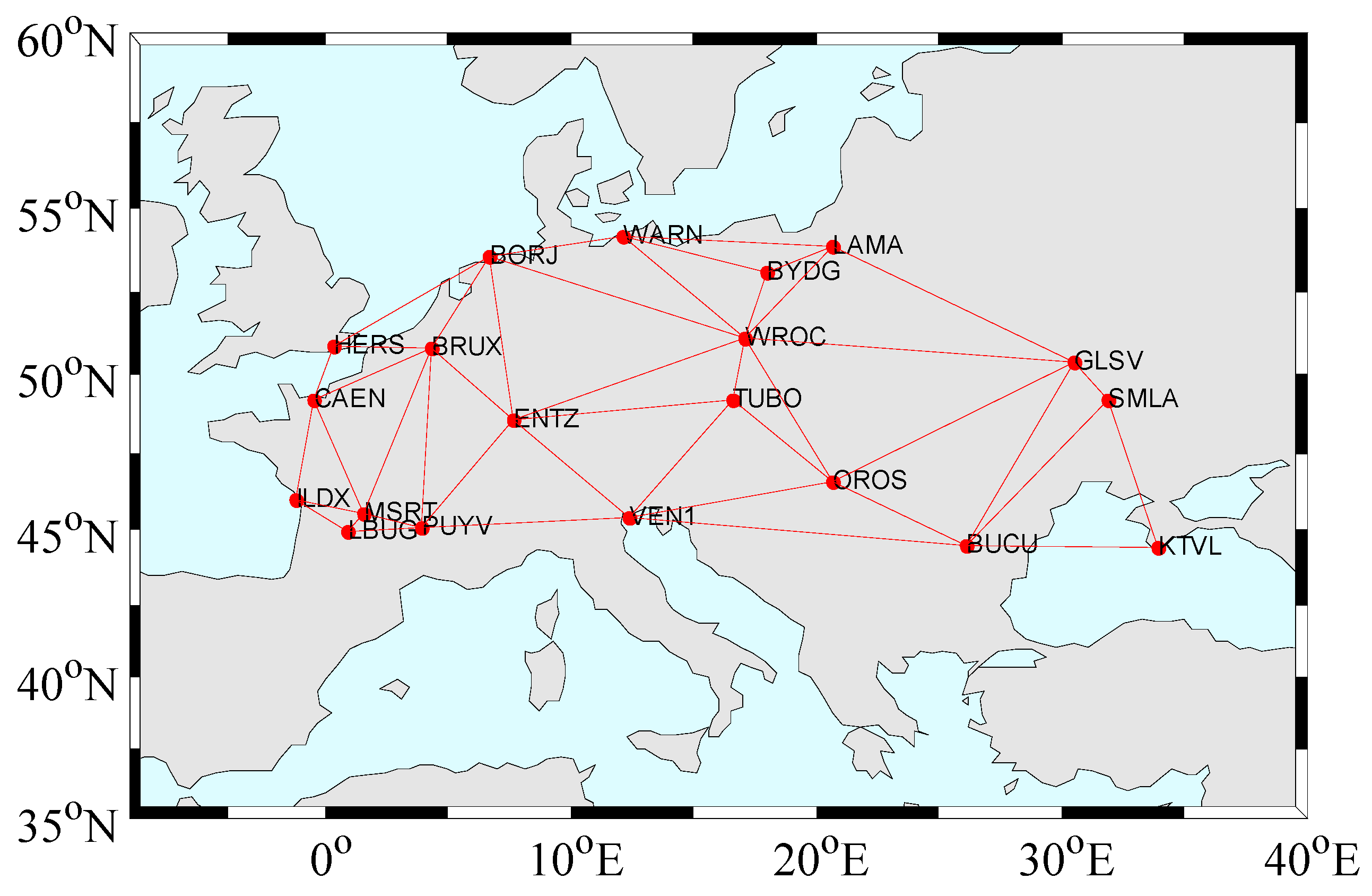
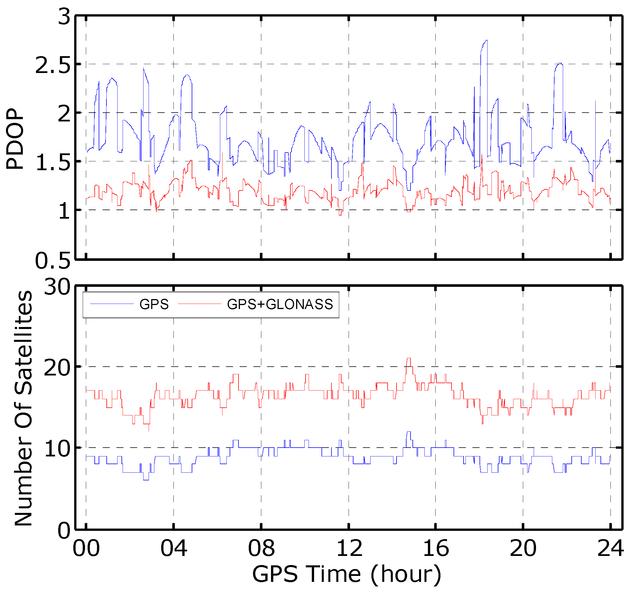
Three weeks (day of year 001–021, 2013) of data collected by 20 stations from the EUREF Permanent GNSS Network were processed to assess the performance of the proposed method. The sampling interval was 30 s. The 20 selected stations are equipped with receivers from different manufacturers and a variety of antennas, domes and firmware versions, which are all detailed in Table 1. We formed 44 baselines, the length of which varied from 81 km to 1090 km and averaged 485.5 km. The distribution of these stations and baselines is shown in Figure 1. There are 24 satellites in operation under the current constellation, and all of them can be observed by the used network. Figure 2 shows the number of satellites and position dilution of precision (PDOP) values for GPS only and GPS+GLONASS. It is seen that, after adding GLONASS, the number of satellites increases from 6–12 to 12–21 while the PDOP value reduces from 1.2–2.7 to 0.9–1.6.
The proposed method was implemented in the PANDA software to carry out the experiment [8]. Final orbit and clock products that were generated at the European Space Agency/European Space Operations Centre (ESA/ESOC) analysis center were used for both GPS and GLONASS. We applied absolute antenna phase center corrections and phase wind-up effects corrections. The station displacements were corrected in accordance with International Earth Rotation and Reference Systems Service (IERS) 2010 conventions. The elevation cutoff angle was set at 7° for each system and the measurements were weighted using an elevation-dependent weighting strategy. We set equal weights for the carrier phase observations of each system but reduced the weight of the GLONASS code observations by a factor of 2.0 when compared with that of GPS. A GPS receiver clock plus an inter-system bias parameter were estimated and a common tropospheric zenith wet delay was estimated as a piecewise constant every 60 min using a global mapping function [45]. The ambiguity parameters and the static position parameters were modeled as constants.
4. Results
In this section, the wide- and narrow-lane ambiguity fixing efficiencies of the proposed method for GLONASS long baseline processing with heterogeneous receivers are validated in detail.
4.1. Deficiency of the Traditional Method
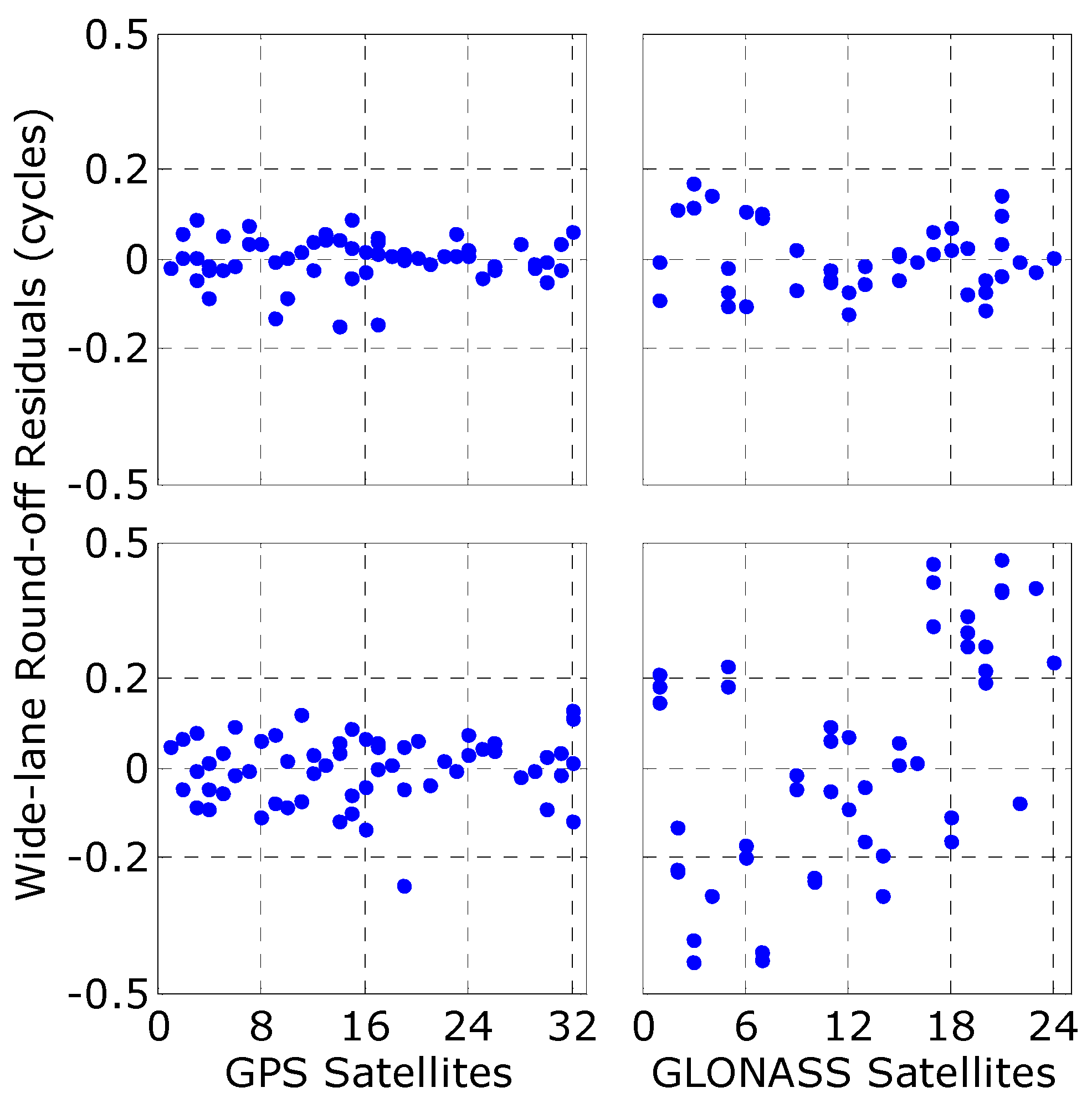
Among the available baselines, we selected one baseline with two homogeneous Trimble receivers and a second baseline with Leica and Trimble receivers. Daily static processing was carried out for each baseline, and Figure 3 shows the round-off residuals of the wide-lane ambiguity that were derived from the HMW combinations. The figure shows that for both baselines, the GPS wide-lane round-off residuals are all within 0.2 cycles, with the exception of only one outlier. For the baseline with the homogeneous receivers, the GLONASS wide-lane round-off residuals are comparable with those of GPS, which are also all within 0.2 cycles. For the baseline with the heterogeneous receivers, however, the GLONASS residuals are randomly distributed within 0.5 cycles, which means we cannot retrieve the integer property of the wide-lane ambiguity.
For further assessment of the HMW-based wide-lane ambiguity resolution performance, a daily static solution was performed for all baselines, and the round-off residuals of both the GPS and GLONASS wide-lane SDBR ambiguities from all baselines over a 21-day period were analyzed. Figure 4a shows the distributions of the wide-lane round-off residuals. Over 96% of the round-off residuals for GPS were smaller than 0.2 cycles. In contrast, only 55% of the round-off residuals for GLONASS were below 0.2 cycles, and the residuals were dispersed within a distribution of 0.5 cycles. The analysis indicates that the GLONASS IFCB cannot be eliminated using the SDBR, and the HMW ambiguity resolution approach is not applicable to GLONASS.
4.2. Efficiency of the Improved Method
In this subsection, we assess the proposed method in detail. The ambiguity connection strategy is introduced to reduce the influence of the residual ionosphere delay, which is based on the fact that the SDBR wide-lane ambiguity difference between two different arcs of the same satellite is an integer. The quality of the ambiguity connection can be assessed by examining the round-off residuals when connecting wide-lane ambiguities. For comparison, we applied the ambiguity connection strategy to both GPS and GLONASS. Figure 4b shows the statistical histogram for these residuals. The figure shows that the residuals are comparable for GPS and GLONASS: 70.3% and 69.1% of the residuals are within 0.1 cycles for GPS and GLONASS, respectively; in addition, 93.8% and 92.6% of the residuals are within 0.2 cycles for GPS and GLONASS, respectively. This means that more than 96% of the small arcs of a single satellite can be connected for both GPS and GLONASS. These statistics thus confirm that the wide-lane ambiguity connection is of good quality.
For comparison, we performed GPS and GLONASS SDBR ambiguity fixing using the following three solutions: GPS using HMW (GPS-HMW), GLONASS using WLP without wide-lane ambiguity connection (GLO-WLP-No) and GLONASS using WLP with wide-lane ambiguity connection (GLO-WLP). Figure 5a shows the distributions of the a posteriori residuals of the wide-lane ambiguities. 81.1% of the GPS-HMW wide-lane residuals were within 0.1 cycles, while 97.1% were within 0.2 cycles. For the GLO-WLP-No wide-lane residuals, only 52.3% and 77.2% were within 0.1 cycles and 0.2 cycles, respectively. We believe that these differences were caused by large residual ionospheric delays. When the wide-lane ambiguity connection was applied, the corresponding percentages improved to 78.0% and 95.5%, respectively, which are comparable to the results from the GPS-HMW solution.
After fixing of the wide-lane ambiguity, the narrow-lane ambiguity was also fixed using the three corresponding solution types. The distributions of the a posteriori residuals of the narrow-lane ambiguities are shown in the Figure 5b. As the figure shows, similar features were found for the distributions of the narrow-lane residuals. For the GPS-HMW and GLO-WLP solutions, more than 87% and 96% of the narrow-lane residuals were within 0.1 cycles and 0.2 cycles, respectively. As expected, if we did not connect the wide-lane ambiguities, the percentages that were within 0.1 cycles and 0.2 cycles degraded to 77.9% and 87.3%, respectively.
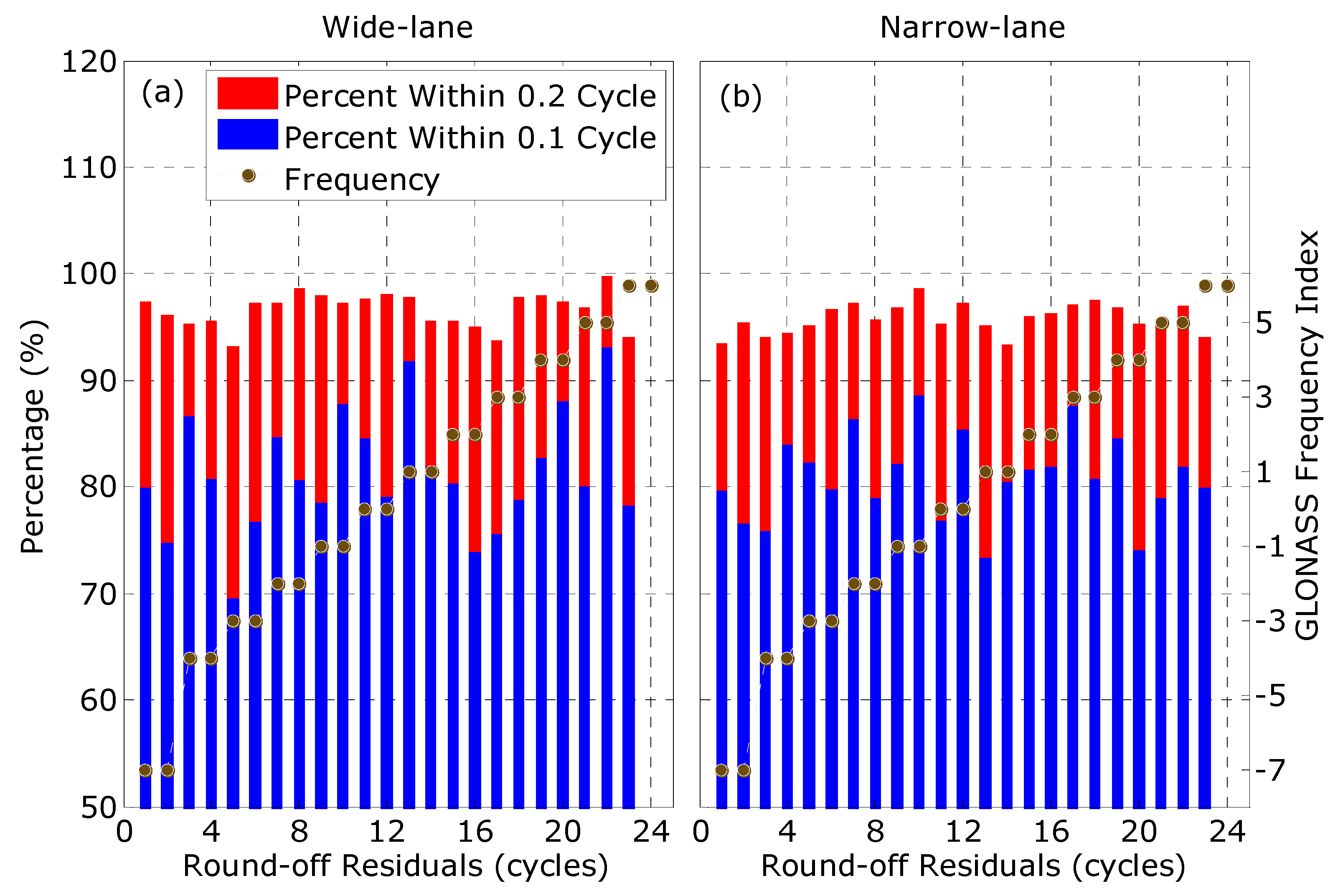
To explore the efficiency of the proposed method in eliminating the effects of GLONASS IFCB on wide-lane ambiguity fixing further, we then calculated the fixing percentages of each GLONASS satellite using the GLO-WLP solution; the results are shown in Figure 6a. At the round-off criterion of 0.1 cycles, the fixing percentages of the different GLONASS satellites when sequenced by frequency number varied widely and randomly, from 73.8% to 82.6%, and averaged a value of 78.1% over all the satellites. The figure also displays a stable and outstanding fixing percentage under the criterion of 0.2 cycles, which fluctuated between approximately 93.8% and 97.2%, with an average of 95.5%. It can thus be concluded that, when using the proposed method, the GLONASS IFCB will have no effect on wide-lane ambiguity fixing, and the fixing percentage will show no relationship with the satellite frequency number.
The corresponding fixing percentages for the narrow-lane ambiguities when using the GLO-WLP solution are shown in Figure 6b, which displays a similar pattern to that obtained for the wide-lane ambiguity. Under the round-off criterion of 0.1 cycles, more than 82% of the narrow-lane ambiguities can be fixed for each satellite, with an average of 87.8%. When the criterion is increased to 0.2 cycles, the fixing percentage then improves significantly to between 96.3% and 97.8% for each satellite. In addition, we also did not identify any relationship between the fixing percentage and the satellite frequency number.
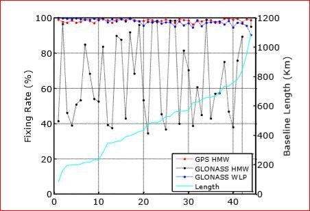
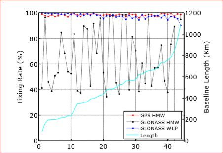
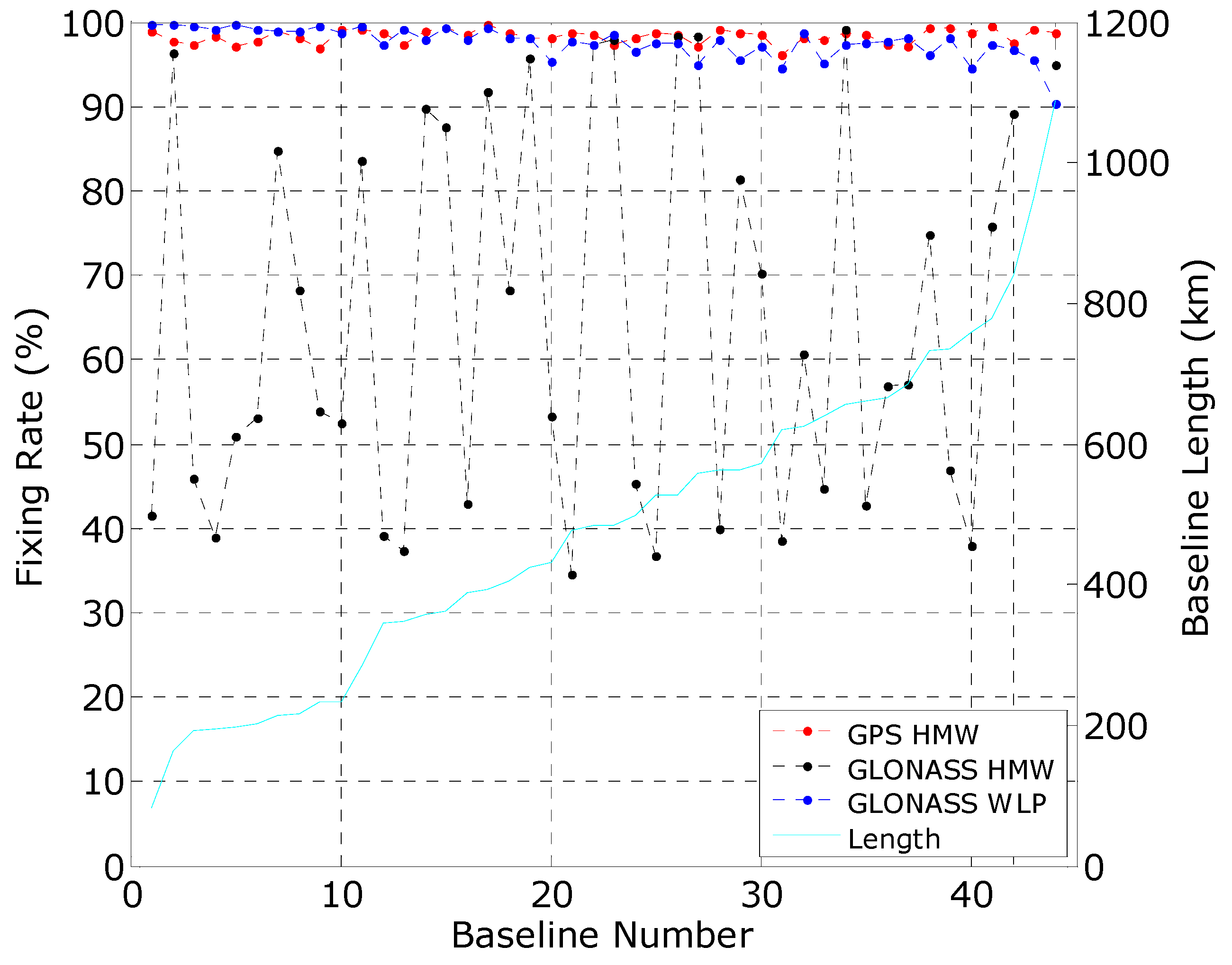
The final fixing rates of the ionospheric-free ambiguity for each baseline are shown in Figure 7. The figure shows that the fixing percentage for the GPS-HMW strategy is more than 96.1% for all baselines, with an average of 98.3%. However, when the HMW method is adopted for GLONASS, the fixing percentages for 16 baselines are below 50% and those for 29 baselines are below 80%. When the proposed method is used, the fixing percentages for all 44 baselines exceed 90%, with an average of 97.5%. Despite the considerable improvements produced using the proposed method, the ambiguity fixing percentage does experience a downward trend with increasing baseline length, which was not observed with the GPS-HMW strategy. For the longest baseline (1089 km), the fixing percentage was only 90.2% for GLONASS, while it was 98.6% for GPS.
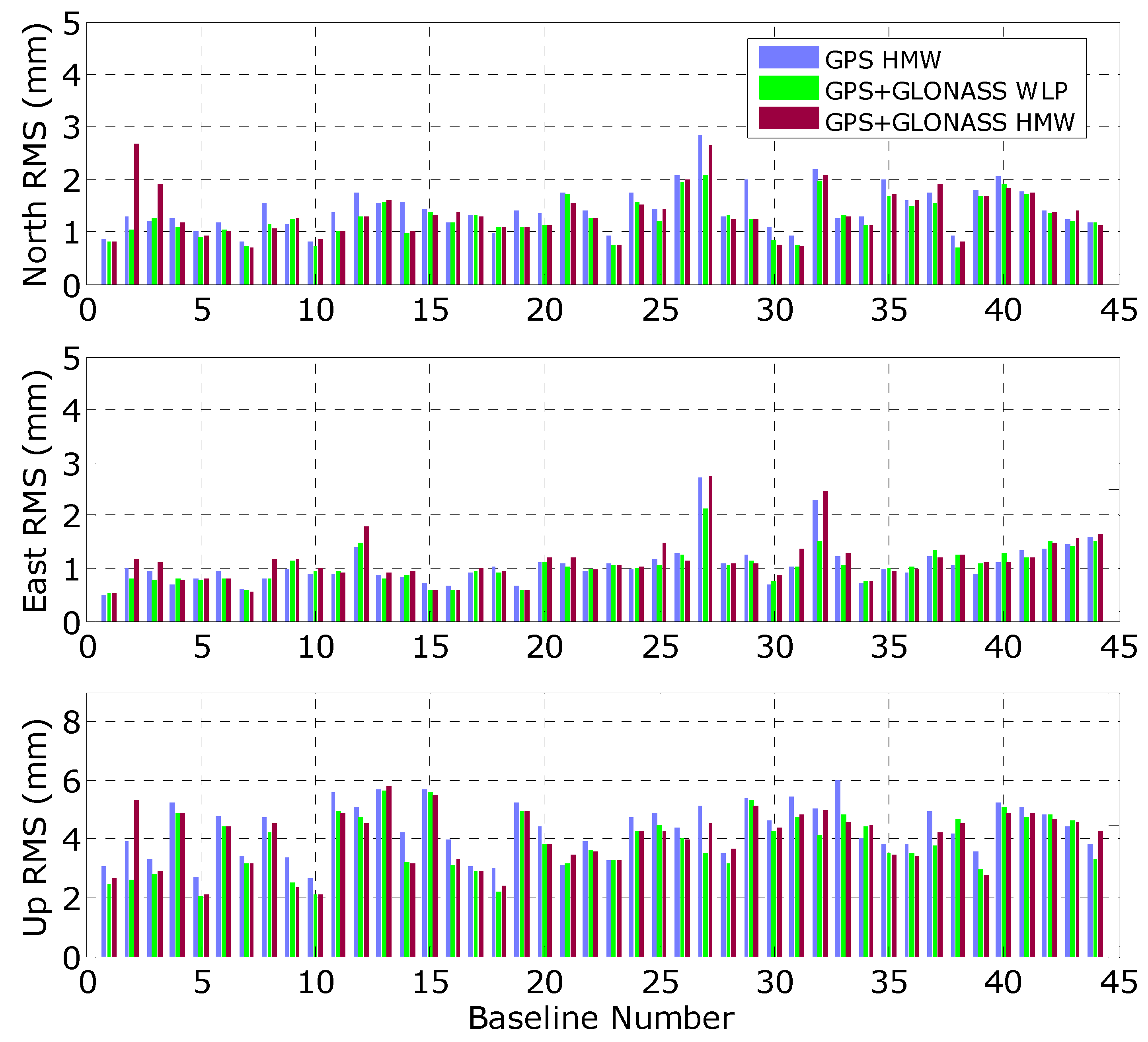
Figure 8 shows the position RMS (root mean square) for GPS-only, GPS+GLONASS with both traditional and the proposed method. The RMS is computed by comparing the baseline estimates with the weekly estimate to assess its accuracy, and is calculated from all the baseline solutions during the 21 days. The baselines have also been arranged with ascending baseline lengths. Compared with the GPS-only solution, regarding the north and up directions there are over 37 baselines for which the RMS is reduced when adding GLONASS with the proposed method, and only 22 for the east direction. Compared with GPS+GLONASS using the proposed method, when using GPS+GLONASS with the traditional method, there are over 30 baselines for which the RMS is enlarged for the north and up directions, and 28 for the east direction. On average, the position RMS was 1.43, 1.06 and 4.32 mm for GPS in the north, east and up directions, respectively. After GLONASS with the proposed method added, the figures reduced to 1.26, 1.02 and 3.87 mm, respectively, with improvements of 11.9%, 3.7% and 10.4%. For both GPS and GLONASS, the satellites moved faster in the north direction than the east, which may cause less improvement in the east when using the combined GPS and GLONASS solution. However, when using the traditional method for GPS+GLONASS, the position RMS was enlarged to 1.35, 1.12 and 4.01 mm, respectively, for the three corresponding directions.
Based on the analysis above, we can confirm the efficiency of the proposed method for use in GLONASS wide- and narrow-lane ambiguity fixing with heterogeneous receivers, in which the effect of the IFCB has been eliminated.
5. Discussion
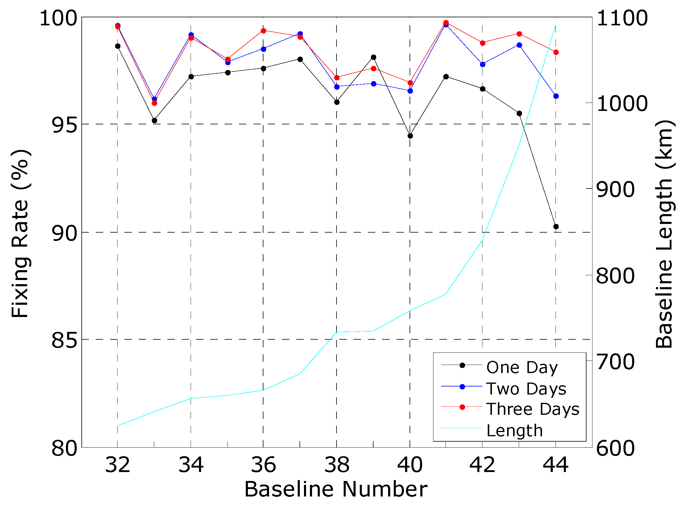
We believe that the reduced fixing percentage for GLONASS shown in Figure 7 is caused by residual ionospheric delays. When the baseline lengths increase, the ionospheric correlation between the two stations decreases, and the residual ionospheric delay will be absorbed directly by the wide-lane ambiguity, which will then affect the WLP-based wide-lane ambiguity fixing process. To improve the fixing percentage of the proposed method over longer baselines, we can use multi-day data for the baseline processing, which means that we can have more arcs from different time spans for each satellite. Because the GIM model has different precisions at different times, the residual ionospheric delays during these different time spans will also vary. Therefore, if we connect these ambiguities from one satellite with the ionospheric-free HMW combination, we will only have to estimate one wide-lane ambiguity for this satellite, and the residual ionospheric delay will thus be greatly reduced.
To verify this theory, we performed GPS+GLONASS long baseline ambiguity resolution using the proposed strategy with data from one-day, two-day, and three-day periods, and the fixing percentages for GLONASS were as shown in Figure 9. It is obvious that the downward trend weakens considerably when the observation data were processed with a two-day interval. For all long baselines, and even for the 1100 km baseline, at least 96% of the SDBR ambiguities can be fixed. When the observation time duration was prolonged to three days, almost no apparent decline in the wide-lane resolution rate was observed with increasing baseline length.
6. Conclusions
As a result of the system’s use of an FDMA strategy, GLONASS code observation is affected by the inter-frequency code bias, which prevents wide-lane ambiguity fixing using the traditional HMW combination. Current studies have not well solved GLONASS ambiguity resolution problem over long baselines. This study has proposed an improved method for GLONASS long baseline ambiguity fixing when using mixed receiver types.
Based on the single-differencing between-receivers processing model, a wide-lane phase combination-based model is proposed in this work to fix the GLONASS ambiguities over long baselines. External precise ionospheric products are introduced to eliminate the ionospheric delays. We connect the wide-lane ambiguities of the different arcs for each GLONASS satellite using the ionospheric-free HMW combination, which means that only one wide-lane ambiguity needs to be estimated for each GLONASS satellite, and the effects of the residual ionospheric delays can also be mitigated in this process.
The round-off residuals were analyzed to assess the performance of the proposed method. When using the traditional HMW method, 96% of the wide-lane round-off residuals were smaller than 0.2 cycles for GPS, as compared with only 55% for GLONASS. When the proposed method was used, the corresponding percentage improved to 95.5% for GLONASS. It was also noted that if the wide-lane ambiguity connection was not applied, the percentage for GLONASS was then only 77.2%. After wide-lane fixing, more than 96% of the narrow-lane ambiguities can be resolved under the criterion of 0.2 cycles for both GPS and GLONASS. In addition, no correlation was observed between the fixing rate and the satellite frequency number for either the wide- or narrow-lane ambiguities. After addition of GLONASS with fixed ambiguity, the RMS position errors were significantly reduced to 1.26, 1.02 and 3.87 mm, representing improvements of 11.9%, 3.7% and 10.4%, for the north, east and up directions, respectively.
The precision of the ionospheric model is the key to this method. In our future research, we intend to focus on establishment of a precise ionospheric model using multi-GNSS observations to assist with GLONASS wide-lane ambiguity resolution. Besides GPS and GLONASS, Galileo and BeiDou have also been establishing their global services. Recently, there has been research on combining Galileo or BeiDou with GPS for medium to long baseline positioning [46,47,48,49]. In future research we will also study the ambiguity resolution performance of Galileo and BeiDou in long baseline positioning.
Author Contributions
J.Z. performed the experiments. Y.L. conceptualized the initial idea and the experimental design. B.W. wrote the main manuscript text. S.Y. helped with data collection and analysis of the results.
Funding
This work was partially supported by the National Natural Science Foundation of China (Grant No. 41704033), the Shenzhen Future Industry Development Funding Program (Grant No. 201607281039561400), the Shenzhen Scientific Research and Development Funding Program (Grant No. JCYJ20170818092931604), and the Research Program of Shenzhen S&T Innovation Committee (Grant No. JCYJ20170412105839839).
Conflicts of Interest
The authors declare no conflict of interest.
References
- Soler, T.; Michalak, P.; Weston, N.; Snay, R.; Foote, R. Accuracy of OPUS solutions for 1- to 4-h observing sessions. GPS Solut. 2006, 10, 45–55. [Google Scholar] [CrossRef]
- Blewitt, G. Carrier phase ambiguity resolution for the global positioning system applied to geodetic baselines up to 2000 km. J. Geophys. Res. 1989, 94, 10187–10203. [Google Scholar] [CrossRef]
- Árnadóttir, T.; Jiang, W.; Feigl, K.L.; Geirsson, H.; Sturkell, E. Kinematic models of plate boundary deformation in southwest Iceland derived from GPS observations. J. Geophys. Res. 2006, 111. [Google Scholar] [CrossRef] [Green Version]
- Haase, J.; Ge, M.; Vedel, H.; Calais, E. Accuracy and variability of GPS tropospheric delay measurements of water vapor in the western mediterranean. J. Appl. Meteorol. 2003, 42, 1547–1568. [Google Scholar] [CrossRef]
- Pacione, R.; Vespe, F. Comparative studies for the assessment of the quality of near-real-time GPS-derived atmospheric parameters. J. Atmos. Ocean. Technol. 2008, 25, 701–714. [Google Scholar] [CrossRef]
- Dach, R.; Lutz, S.; Walser, P.; Fridez, P. Bernese GNSS Software Version 5.2. User Manual; Astronomical Institute, Universtiy of Bern, Bern Open Publishing: Bern, Switzerland, 2015; ISBN 978-3-906813-05-9. [Google Scholar] [CrossRef]
- Herring, T.; King, R.; McClusky, S. GAMIT Reference Manual: GPS Analysis at MIT; Release 10.4; Department of Earth, Atmospheric, and Planetary Sciences, Massachusset Institute of Technology: Cambridge, MA, USA, 2010. [Google Scholar]
- Shi, C.; Zhao, Q.; Lou, Y. Recent development of PANDA software in GNSS data processing. Proc. SPIE 2008, 7285, 231–249. [Google Scholar]
- Dow, J.; Neilan, R.; Rizos, C. The international GNSS service in a changing landscape of global navigation satellite systems. J. Geod. 2009, 83, 191–198. [Google Scholar] [CrossRef]
- Dilssner, F.; Springer, T.; Gienger, G.; Dow, J. The GLONASS-M satellite yaw-attitude model. Adv. Space Res. 2010, 47, 160–171. [Google Scholar] [CrossRef]
- Raby, P.; Daly, P. Using the GLONASS system for geodetic surveys. In Proceedings of the 6th International Technical Meeting of the Satellite Division of the Institute of Navigation, Salt Lake City, UT, USA, 22–24 September 1993; pp. 1129–1138. [Google Scholar]
- Pratt, M.; Burke, B.; Misra, P. Single-epoch integer ambiguity resolution with GPS-GLONASS L1-L2 Data. In Proceedings of the ION GPS-98, Nashville Convention Center, TN, USA, 15–18 September 1998; pp. 691–699. [Google Scholar]
- Leick, A. GLONASS satellite surveying. J. Surv. Eng. 1998, 124, 91–99. [Google Scholar] [CrossRef]
- Dai, L.; Han, S.; Rizos, C. A new data processing strategy for combined GPS/GLONASS carrier phase-based positioning. In Proceedings of the 12th International Technical Meeting of the Satellite Division of the U.S. Institution of Navigation, Nashville, TN, USA, 14–17 September 1999; pp. 1619–1627. [Google Scholar]
- Wang, J.; Leick, A.; Rizos, C.; Stewart, M. GPS and GLONASS integration: Modeling and ambiguity resolution issues. GPS Solut. 2001, 5, 55–64. [Google Scholar] [CrossRef]
- Leick, A. GPS Satellite Surveying; Wiley: New York, NY, USA, 1995; p. 560. [Google Scholar]
- Landau, H.; Vollath, U. Carrier phase ambiguity resolution using GPS and GLONASS signals. In Proceedings of the 9th International Technical Meeting of the Satellite Division of the U.S. Institution of Navigation GPS ION’96, Kansas City, MO, USA, 17–20 September 1996; pp. 917–923. [Google Scholar]
- Takasu, T.; Yasuda, A. Development of the low-cost RTK-GPS receiver with an open source program package RTKLIB. In Proceedings of the International Symposium on GPS/GNSS, Seogwipo-si Jungmun-dong, Korea, 4–6 November 2009. [Google Scholar]
- Al-Shaery, A.; Zhang, S.; Rizos, C. An enhanced calibration method of GLONASS inter-channel bias for GNSS RTK. GPS Solut. 2013, 17, 165–173. [Google Scholar] [CrossRef]
- Povalyaev, A. Using single differences for relative positioning in GLONASS. In Proceedings of the 10th International Technical Meeting of the Satellite Division of the U.S. Institution of Navigation, Kansas, MO, USA, 16–19 September 1997; pp. 929–934. [Google Scholar]
- Cao, W.; O’Keefe, K.; Cannon, M. Performance Evaluation of GPS/Galileo Multiple-frequency RTK Positioning Using a Single-difference Processor. In Proceedings of the ION GNSS 2008, Savannah, GA, USA, 16–19 September 2008; pp. 2841–2849. [Google Scholar]
- Feng, Y.; Li, B. Four Dimensional Real Time Kinematic State Estimation and Analysis of Relative Clock Solutions. In Proceedings of the ION GNSS 2010, Portland, OR, USA, 21–24 September 2010; pp. 2092–2099. [Google Scholar]
- Liu, Y.; Ye, S.; Jiang, P.; Song, W.; Lou, Y. Combining GPS+GLONASS observations to improve the fixing percentage and precision of long baselines with limited data. Adv. Space Res. 2016, 57, 1258–1267. [Google Scholar] [CrossRef]
- Wanninger, L.; Wallstab-Freitag, S. Combined GPS, GLONASS, and SBAS code phase and carrier phase measurements. In Proceedings of the 20th International Technical Meeting of the Satellite Division of the U.S. Institution of Navigation, Fort Worth, TX, USA, 25–28 September 2007; pp. 866–875. [Google Scholar]
- Sleewaegen, J.; Simsky, A.; de Wilde, W.; Boon, F.; Willems, T. Demystifying GLONASS inter-frequency carrier phase biases. InsideGNSS 2012, 7, 57–61. [Google Scholar]
- Wanninger, L. Carrier phase inter-frequency biases of GLONASS receivers. J. Geod. 2012, 86, 139–148. [Google Scholar] [CrossRef]
- Kozlov, D.; Tkachenko, M.; Tochilin, A. Statistical characterisation of hardware biases in GPS+GLONASS receivers. In Proceedings of the 13th International Technical Meeting of the Satellite Division of the U.S. Institution of Navigation, Salt Lake City, UT, USA, 19–22 September 2000; pp. 817–826. [Google Scholar]
- Yamada, H.; Takasu, T.; Kubo, N.; Yasuda, A. Evaluation and calibration of receiver inter-channel biases for RTK-GPS/GLONASS. In Proceedings of the ION GNSS-2010, Portland, OR, USA, 21–24 September 2010; pp. 1580–1587. [Google Scholar]
- Reussner, N.; Wanninger, L. GLONASS Inter-frequency Biases and Their Effects on RTK and PPP Carrier phase Ambiguity Resolution. In Proceedings of the ION GNSS 2011, Institute of Navigation, Portland, OR, USA, 19–23 September 2011; pp. 712–716. [Google Scholar]
- Banville, S.; Collins, P.; Lahaye, F. Concepts for undifferenced GLONASS ambiguity resolution. In Proceedings of the 26th International Technical Meeting of the Satellite Division of The Institute of Navigation (ION GNSS+ 2013), Nashville, TN, USA, 16–20 September 2013; pp. 1186–1197. [Google Scholar]
- Chuang, S.; Yi, W.; Song, W.; Lou, Y.; Zhang, R. GLONASS pseudorange inter-channel biases and their effects on combined GPS/GLONASS precise point positioning. GPS Solut. 2013, 17, 439–451. [Google Scholar] [CrossRef]
- Hatch, R. The synergism of GPS code and carrier measurements. In Proceedings of the Third International Symposium on Satellite Doppler Positioning at Physical Sciences Laboratory of New Mexico State University, Las Cruces, NM, USA, 8–12 February 1982; Volume 2, pp. 1213–1231. [Google Scholar]
- Melbourne, W. The case for ranging in GPS-based geodetic systems. In Proceedings of the First International Symposium on Precise Positioning with the Global Positioning System, Rockville, MD, USA, 15–19 April 1985. [Google Scholar]
- Wübbena, G. Software developments for geodetic positioning with GPS using TI-4100 code and carrier measurements. In Proceedings of the First International Symposium on Precise Positioning with the Global Positioning System, Rockville, MD, USA, 5–19 April 1985. [Google Scholar]
- Yi, W. Research on Rapid Convergence and Integer Ambiguity Resolution Method for Multi-GNSS Precise Point Positioning. Ph.D. Thesis, Wuhan University, Wuhan, China, 2015. (In Chinese). [Google Scholar]
- Banville, S. GLONASS ionosphere-free ambiguity resolution for precise point positioning. J. Geod. 2016, 90, 487–496. [Google Scholar] [CrossRef]
- Liu, Y.; Ge, M.; Shi, C.; Lou, Y.; Wickert, J.; Schuh, H. Improving integer ambiguity resolution for GLONASS precise orbit determination. J. Geod. 2016, 90, 715–726. [Google Scholar] [CrossRef]
- Geng, J.; Zhao, Q.; Shi, C.; Liu, J. A review on the inter-frequency biases of GLONASS carrier-phase data. J. Geod. 2016, 91, 329–340. [Google Scholar] [CrossRef]
- Geng, J.; Bock, Y. GLONASS fractional-cycle bias estimation across inhomogeneous receivers for PPP ambiguity resolution. J. Geod. 2015. [Google Scholar] [CrossRef]
- Yi, W.; Song, W.; Lou, Y.; Shi, C.; Yao, Y. A method of undifferenced ambiguity resolution for GPS+GLONASS precise point positioning. Sci. Rep. 2016, 6, 26334. [Google Scholar] [CrossRef] [PubMed] [Green Version]
- Liu, Y.; Gu, S.; Li, Q. Calibration of glonass inter-frequency code bias for PPP ambiguity resolution with heterogeneous rover receivers. Remote Sens. 2018, 10, 399. [Google Scholar] [CrossRef]
- Liu, Y.; Song, W.; Lou, Y.; Ye, S.; Zhang, R. Glonass phase bias estimation and its PPP ambiguity resolution using homogeneous receivers. GPS Solut. 2016. [CrossRef]
- Liu, Y.; Ye, S.; Song, W.; Lou, Y.; Gu, S.; Li, Q. Rapid PPP Ambiguity Resolution Using GPS+GLONASS Observations. J. Geod. 2016. [Google Scholar] [CrossRef]
- Hernández-Pajares, M.; Juan, J.; Sanz, J.; Orús, R.; Garcia-Rigo, A.; Feltens, J.; Komjathy, A.; Schaer, S.; Krankowski, A. The IGS VTEC maps: A reliable source of ionospheric information since 1998. J. Geod. 2009, 83, 263–275. [Google Scholar] [CrossRef]
- Boehm, J.; Niell, A.; Tregoning, P.; Schuh, H. Global mapping function (GMF): A new empirical mapping function based on numerical weather model data. Geophys. Res. Lett. 2006, 33, L07304. [Google Scholar] [CrossRef]
- Gao, W.; Gao, C.; Pan, S.; Meng, X.; Xia, Y. Inter-system differencing between GPS and BDS for medium-baseline RTK positioning. Remote Sens. 2017, 9, 948. [Google Scholar] [CrossRef]
- Li, G.; Geng, J.; Guo, J.; Zhou, S.; Lin, S. GPS + Galileo tightly combined RTK positioning for medium-to-long baselines based on partial ambiguity resolution. J. Glob. Position. Syst. 2018, 16, 3. [Google Scholar] [CrossRef]
- Yalvac, S.; Berber, M. Galileo satellite data contribution to GNSS solutions for short and long baselines. Measurement 2018, 124, 173–178. [Google Scholar] [CrossRef]
- Paziewski, J.; Sieradzki, R.; Wielgosz, P. On the Applicability of Galileo FOC Satellites with Incorrect Highly Eccentric Orbits: An Evaluation of Instantaneous Medium-Range Positioning. Remote Sens. 2018, 10, 208. [Google Scholar] [CrossRef]
Figure 1.
Distribution of the stations used and the baselines.

Figure 2.
Satellite number and PDOP (position dilution of precision) values for Global Positioning System (GPS) only and GPS+Globalnaya Navigatsionnaya Sputnikovaya Sistema (GLONASS) at one station (TUBO) in the center of the network on day of year 001 in 2013.
Figure 2.
Satellite number and PDOP (position dilution of precision) values for Global Positioning System (GPS) only and GPS+Globalnaya Navigatsionnaya Sputnikovaya Sistema (GLONASS) at one station (TUBO) in the center of the network on day of year 001 in 2013.

Figure 3.
Round-off residuals of wide-lane single-differencing between-receivers (SDBR) ambiguities of GPS and GLONASS satellites for a baseline with homogeneous receivers (top) and a baseline with heterogeneous receivers (bottom).
Figure 3.
Round-off residuals of wide-lane single-differencing between-receivers (SDBR) ambiguities of GPS and GLONASS satellites for a baseline with homogeneous receivers (top) and a baseline with heterogeneous receivers (bottom).

Figure 4.
Distributions of a posteriori residuals for GPS and GLONASS when performing wide-lane ambiguity fixing (a) and connection (b) using the Hatch–Melbourne–Wubbena (HMW) combination.
Figure 4.
Distributions of a posteriori residuals for GPS and GLONASS when performing wide-lane ambiguity fixing (a) and connection (b) using the Hatch–Melbourne–Wubbena (HMW) combination.
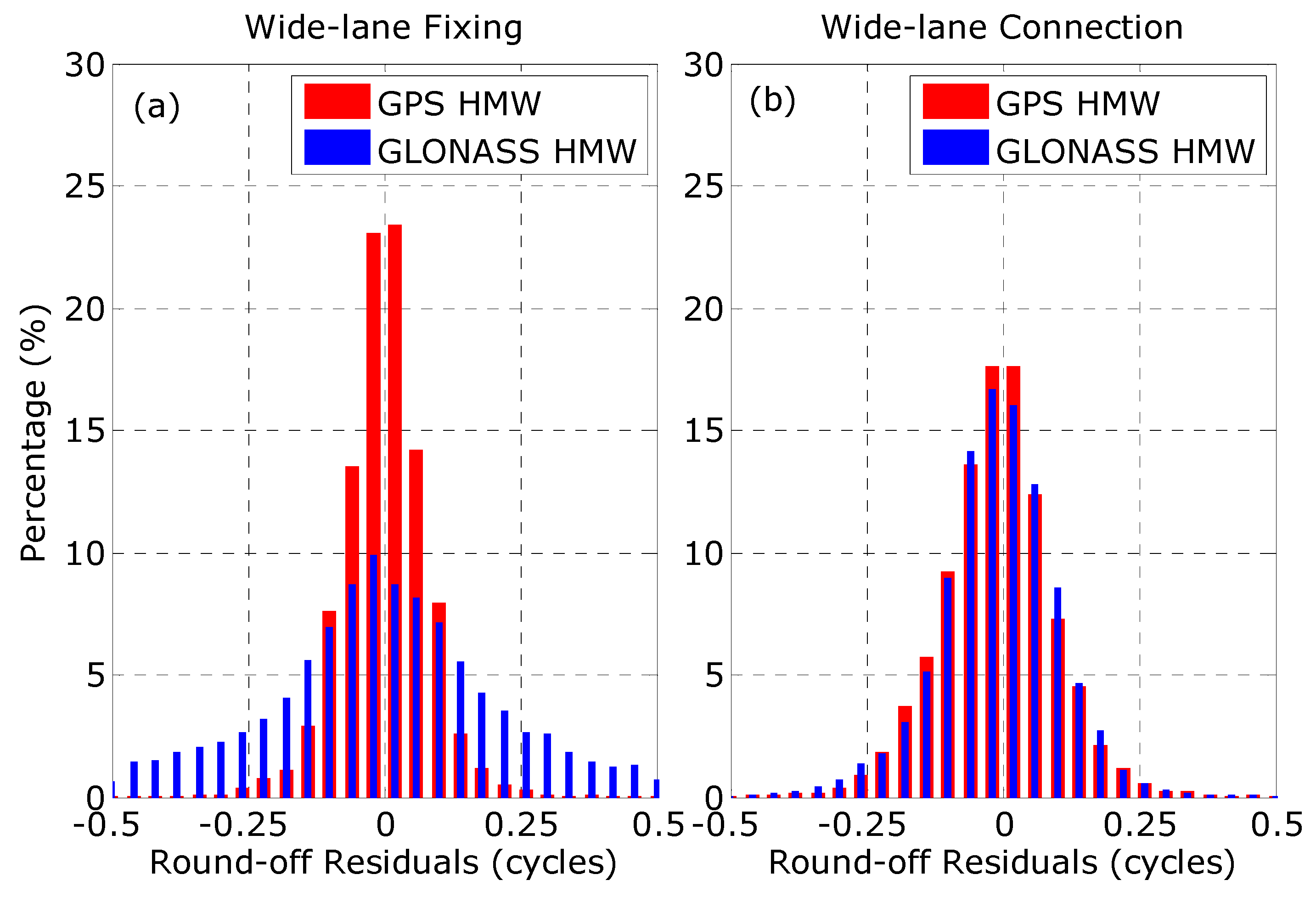
Figure 5.
Distributions of the a posteriori residuals in GPS and GLONASS wide- and narrow-lane SDBR ambiguities fixing using the HMW and the WLP (wide-lane phase) combinations. (a) It shows the distributions of the a posteriori residuals of the wide-lane ambiguities; (b) It shows the distributions of the a posteriori residuals of the narrow-lane ambiguities.
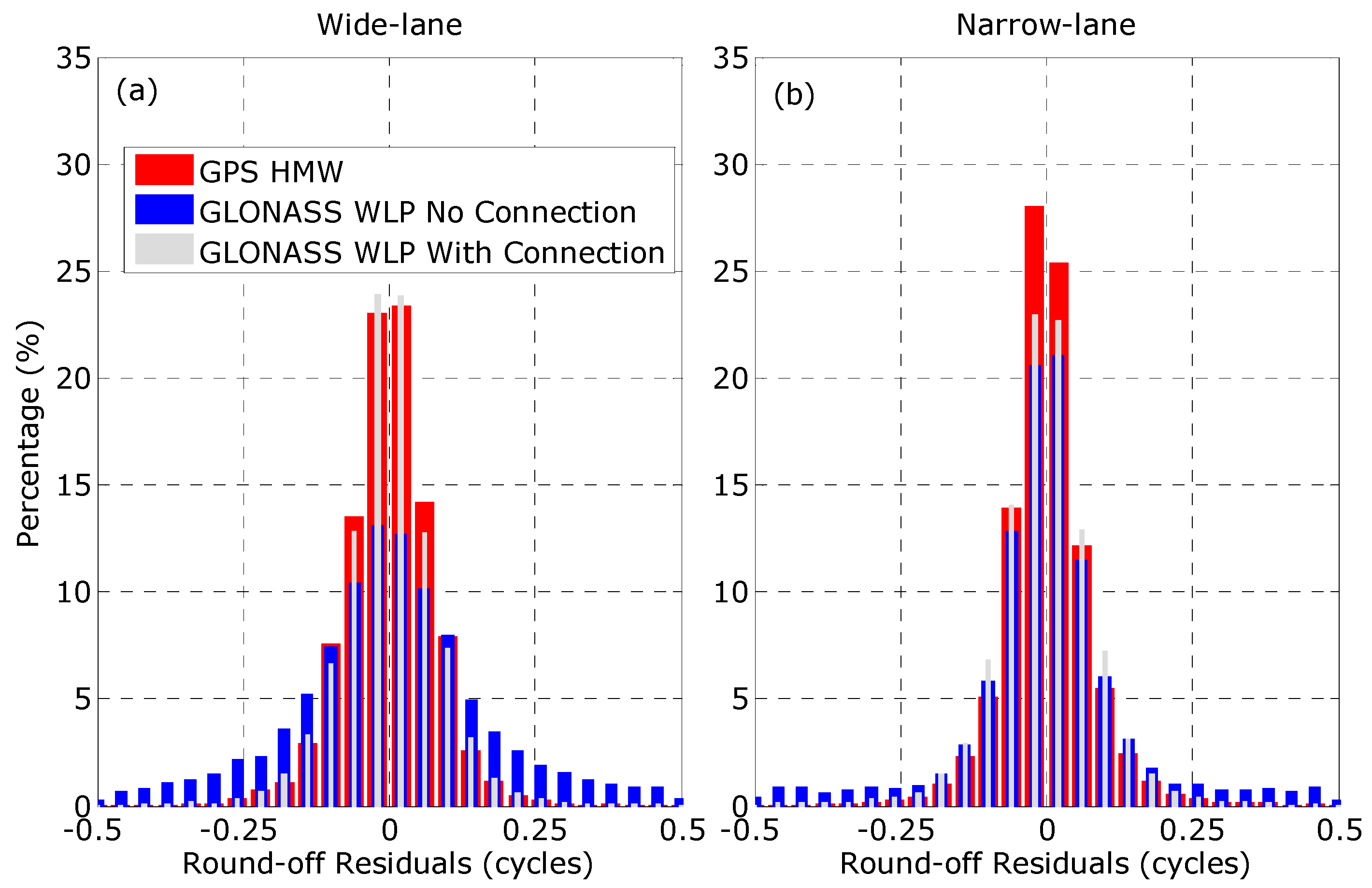
Figure 6.
Percentages within 0.1 and 0.2 cycles for the a posteriori residuals in GLONASS wide- and narrow-lane SDBR ambiguities fixing when using the proposed method. (a) It shows the corresponding fixing percentages for the wide-lane ambiguities. (b) It shows the corresponding fixing percentages for the narrow-lane ambiguities.

Figure 7.
Fixing percentages of the ionospheric-free ambiguities for all baselines. The results show that the proposed method can achieve fixing rates for GLONASS that are comparable to those of GPS.
Figure 7.
Fixing percentages of the ionospheric-free ambiguities for all baselines. The results show that the proposed method can achieve fixing rates for GLONASS that are comparable to those of GPS.

Figure 8.
Position RMS (root mean square) for the GPS Only and GPS+GLONASS daily static baseline solutions.
Figure 8.
Position RMS (root mean square) for the GPS Only and GPS+GLONASS daily static baseline solutions.

Figure 9.
Improvements in the fixing percentage when using the proposed method with multi-day observation data.
Figure 9.
Improvements in the fixing percentage when using the proposed method with multi-day observation data.

Table 1.
Technical details of the 20 tracking stations used with various hardware configurations.
| Manufacturer | Receiver | Antenna | Dome | Firmware | Stations |
|---|---|---|---|---|---|
| Trimble | NETR5 | TRM55971.00 | NONE | 4.42 | CAEN |
| 4.48 | ENTZ PUYV | ||||
| TZGD | Nav 4.41/Boot 4.18 | BYDG | |||
| NETR9 | TRM57971.00 | NONE | 4.60 | ILDX | |
| Leica | GRX1200GGPRO | LEIAT504GG | LEIS | 8.10/3.019 | BUCU |
| NONE | 8.51/3.019 | VEN1 | |||
| GRX1200+GNSS | LEIAR25.R3 | LEIT | 8.51/6.110 | OROS | |
| LEIAR25.R4 | LEIT | 8.51/6.110 | TUBO | ||
| LEIAT504GG | LEIS | 8.10/4.007 | LAMA | ||
| LEICA GR25 | LEIAR25.R4 | LEIT | 2.62/6.112 | WROC | |
| Novatel | OEMV3 | NOV702GG | NONE | 3.701 | GLSV SMLA |
| 3.620 | KTVL | ||||
| TPS | NETG3 | TPSCR.G3 | TPSH | 3.4 | MSRT LBUG |
| JPS | LEGACY | LEIAR25.R3 | LEIT | 2.6.1 JAN,10,2008 | BORJ WARN |
| Septentrio | POLARX4TR | JAVRINGANT_DM | NONE | 2.3.4 | BRUX |
| POLARX3ETR | LEIAR25.R3 | NONE | 2.1 | HERS |
© 2018 by the authors. Licensee MDPI, Basel, Switzerland. This article is an open access article distributed under the terms and conditions of the Creative Commons Attribution (CC BY) license (http://creativecommons.org/licenses/by/4.0/).
Share and Cite
MDPI and ACS Style
Zhu, J.; Liu, Y.; Wang, B.; Ye, S. Improved Method for GLONASS Long Baseline Ambiguity Resolution without Inter-Frequency Code Bias Calibration. Remote Sens. 2018, 10, 1223. https://0-doi-org.brum.beds.ac.uk/10.3390/rs10081223
AMA Style
Zhu J, Liu Y, Wang B, Ye S. Improved Method for GLONASS Long Baseline Ambiguity Resolution without Inter-Frequency Code Bias Calibration. Remote Sensing. 2018; 10(8):1223. https://0-doi-org.brum.beds.ac.uk/10.3390/rs10081223
Chicago/Turabian StyleZhu, Jiasong, Yanyan Liu, Bing Wang, and Shirong Ye. 2018. "Improved Method for GLONASS Long Baseline Ambiguity Resolution without Inter-Frequency Code Bias Calibration" Remote Sensing 10, no. 8: 1223. https://0-doi-org.brum.beds.ac.uk/10.3390/rs10081223
Note that from the first issue of 2016, this journal uses article numbers instead of page numbers. See further details here.