A CNN-SIFT Hybrid Pedestrian Navigation Method Based on First-Person Vision
by
 , and
, and
Qi Zhao
1 ,
,
Boxue Zhang
1,
Shuchang Lyu
1,
Hong Zhang
2,*,
Daniel Sun
3,
Guoqiang Li
4,* and
Wenquan Feng
1 1
School of Electronic and Information Engineering, Beihang University, Xueyuan Road, Beijing 100191, China
2
Image Processing Center, Beihang University, Xueyuan Road, Beijing 100191, China
3
Data61, CSIRO, Canberra, ACT 2601, Australia
4
School of Software, Shanghai Jiao Tong University, Shanghai 200240, China
*
Authors to whom correspondence should be addressed.
Remote Sens. 2018, 10(8), 1229; https://0-doi-org.brum.beds.ac.uk/10.3390/rs10081229
Submission received: 11 July 2018
/
Revised: 27 July 2018
/
Accepted: 1 August 2018
/
Published: 5 August 2018
(This article belongs to the Special Issue Instrumenting Smart City Applications with Big Sensing and Earth Observatory Data: Tools, Methods and Techniques)
Abstract
:The emergence of new wearable technologies, such as action cameras and smart glasses, has driven the use of the first-person perspective in computer applications. This field is now attracting the attention and investment of researchers aiming to develop methods to process first-person vision (FPV) video. The current approaches present particular combinations of different image features and quantitative methods to accomplish specific objectives, such as object detection, activity recognition, user–machine interaction, etc. FPV-based navigation is necessary in some special areas, where Global Position System (GPS) or other radio-wave strength methods are blocked, and is especially helpful for visually impaired people. In this paper, we propose a hybrid structure with a convolutional neural network (CNN) and local image features to achieve FPV pedestrian navigation. A novel end-to-end trainable global pooling operator, called AlphaMEX, has been designed to improve the scene classification accuracy of CNNs. A scale-invariant feature transform (SIFT)-based tracking algorithm is employed for movement estimation and trajectory tracking of the person through each frame of FPV images. Experimental results demonstrate the effectiveness of the proposed method. The top-1 error rate of the proposed AlphaMEX-ResNet outperforms the original ResNet (k = 12) by 1.7% on the ImageNet dataset. The CNN-SIFT hybrid pedestrian navigation system reaches 0.57 m average absolute error, which is an adequate accuracy for pedestrian navigation. Both positions and movements can be well estimated by the proposed pedestrian navigation algorithm with a single wearable camera.

1. Introduction
Portable cameras, able to record dynamic high quality first person video, have become common equipment among sportsmen, policemen, etc., over the last ten years. These devices represent commercial attempts to record experiences from a first-person perspective. This technological trend is a follow-up of the academic results obtained in the late 1990s [1], with the growing interest of people to record their daily activities. Until now, no consensus has yet been reached in the literature with respect to naming this video perspective. First-person vision (FPV) [2] is arguably the most commonly used, but other names, such as egocentric vision and ego-vision, have also recently grown in popularity. There are many objectives of FPV analysis, such as object recognition and tracking [3,4,5,6], activity recognition [7,8,9,10,11], and environment mapping [12,13,14,15].
FPV-based navigation is generally useful, and necessary in some special areas where Global Position System (GPS) or other radio-wave strength methods are blocked [16]; this is especially true for visually impaired people, who need a localization method that can work in any urban area, ranging from underground to narrow open-sky pavements enclosed by tall buildings. Traditional FPV-based pedestrian navigation can be recognized as a part of a general image retrieval problem of snapshots. Image features are extracted to identify the position of the current frame. Although this enables scene recognition, image extraction is unable to meet the requirements of navigation as it uses no information about the movements of the body, which provides more accurate position estimation [17].
In this paper, we propose a hybrid structure with scene recognition and movement estimation. A novel end-to-end trainable global pooling operator, called AlphaMEX, has been designed to improve the scene recognition accuracy of a convolutional neural network (CNN) [18]. To estimate the wearer’s movement through the FPV, scale-invariant feature transform (SIFT) [19] features are calculated for the key points in consecutive frames, and the matched points between these two frames are extracted. The contributions of this paper can be summarized as follows:
- Based on the proposed AlphaMEX function, an end-to-end trainable global pooling layer is designed, named AlphaMEX Global Pool. This novel global pooling layer has three advantages: First, it improves the performance of state-of-the-art CNN structures without inserting any redundant layers or parameters; second, it is smarter than any traditional global pooling method that could be well trained end-to-end; and, finally, it is more appropriate in modern CNN structures, as the feature-maps become sparse after batch normalization (BN) [20] and rectified linear unit (ReLU) [21] combined layers, which are commonly used in state-of-the-art “non-plain” CNNs.
- A novel iterative structure is designed for pedestrian navigation, which combines the AlphaMEX CNN-based localization and the SIFT-based movement estimation. As the SIFT-based movement estimation requires continuous frames, the iterative structure is appropriate for the hybrid method. Also, an iterative function is indispensable in the road detection algorithm (see Section 4.3). The proposed iterative structure concisely combines both of the characteristics.
- Experimental results on CIFAR [22], Street View House Numbers (SVHN) [23] and ImageNet [24] datasets demonstrate the effectiveness of the AlphaMEX Global Pool. Movement can be well estimated with an adequate accuracy based on the proposed projective geometry algorithm in the model test. In addition, an FPV database named “BuaaFPV” is designed for further validation.
The paper is organized as follows. Section 2 presents related works and conducts a systematic analysis. Section 3 describes our proposed hybrid structure in detail, including its mathematical principles as well as the implementation of the AlphaMEX Global Pool, the SIFT-based movement estimation and the CNN-SIFT hybrid pedestrian navigation structure. The experimental results are systematically analyzed in Section 4. Finally, Section 5 and Section 6 discuss the system and draw conclusions.
2. Related Work
FPV video analysis provides methodological and practical advantages, solves some problems of traditional video analysis and offers extra information. Wearable devices allow the user to record (potentially without detection) the most relevant parts of a scene for analysis, thus reducing the necessity for complex controlled multi-camera systems [25]. According to [26], eye and head movements are directly influenced by a person’s emotional state. As already seen with smartphones [27], this fact can be exploited to infer the user’s emotional state and provide services accordingly. Because users tend to see objects while interacting with them, it is possible to take advantage of the prior knowledge of the hands’ and objects’ positions (e.g., active objects tend to be closer to the center of the frame, whereas hands tend to appear in the bottom-left and bottom-right of the frame) [28,29]. Changes in illumination and global scene characteristics could be used as an important feature to detect the scene in which the user is involved (e.g., detecting changes in the place where the activity is taking place, as in [30]). An intuitive step in the hierarchy of objectives is activity recognition, aimed at identifying where the user is and what he/she is doing in a particular video sequence. Global scene identification, as well as object identification, stand out as two important sub-tasks for activity recognition. Hodges et al. [31] present the “SenseCam”, a multi-sensor device subsequently used for activity recognition. Sundaram et al. [32] model activities as sequences of events using only FPV videos. Ogaki et al. [33] and Poleg et al. [10] used the fact that different activities (e.g., jumping, walking, jogging, skating, writing, and watching TV) generate different motion patterns due to peculiar body motions associated with each activity [1]. Deep learning algorithms such as Mask R-CNN [34] can be used for human pose estimation in FPV.
Selection of suitable features is imperative to exploit the advantages of FPV, as scene attributes and characteristics undergo dynamic changes after FPV application. Features are extracted from pixels, color channels and eventually from frames. Feature extraction at frame level is deemed important for elaborate indicators like texture, gradients, super pixels, etc. [1]. In-depth analysis can be carried out by adding dynamic information in different approaches, which include comparison of geometrical transformation between two frames to acquire motion features (such as optical flow) and aggregation of frame level features in temporal windows. Takizawa et al. [35] proposed a spot navigation system for a visually impaired person by a SIFT-based matching algorithm. Hu et al. [36] combined a two-dimensional navigation algorithm based on extended Kalman filtering with three-dimensional mapping based on a SIFT algorithm to realize a low-cost 3D environment mapping. Dynamic features, being computationally expensive, are generally used in experiments where video processing is introduced after all other activities [1].
CNN have become a powerful approach to deal with the scene identification problem. As a deep learning method, it performs convolution in the lower layers of the network. For classification, the feature maps of the last convolutional layer are vectorized and fed into fully connected layers followed by a softmax logistic regression layer [37,38]. This structure bridges the convolutional structure with traditional neural network classifiers. It treats the convolutional layers as feature extractors, and the resulting feature is classified in a traditional way. Pooling layers between convolutional layers aims to strengthen the translational invariance and reduce the dimension of the feature maps. Max pooling [39], which computes the maximum of a local patch, is one of the typical pooling methods. Another commonly used pooling method is average pooling [40], which outputs the mean value of a local patch. Global average pooling was first used in NIN (network in network) [41] to replace the traditional fully connected layers. The idea is to generate one feature map for each corresponding category of the classification task in the last convolutional layer. Global average pooling is widely used in modern CNN structures for its advantages. Highway networks [42] are amongst the first architectures that provided a means to effectively train end-to-end networks with more than 100 layers. In ResNet [43], pure identity mappings are used as bypassing paths, and it has achieved impressive, record-breaking performances on many challenging image recognition, localization, and detection tasks, such as ImageNet [24] and COCO (Common Objects in Context) object detection [43]. Instead of drawing representational power from extremely deep or wide architectures, DenseNet [44] exploits the potential of the network through feature reuse, yielding condensed models that are easy to train and highly parameter efficient. Concatenating feature-maps learned by different layers increases variation in the input of subsequent layers and improves efficiency.
Cloud computing and edge computing have been de facto platforms for computer vision and image processing applications, including FPV. As a systemic solution, usually we have to take into account both applications and platforms to achieve the best performance [45,46,47,48,49]. In this paper, we focus on the application level and leave the system issues untouched.
3. Materials and Methods
The proposed FPV pedestrian navigation algorithm takes an FPV video sequence as input and gives as output a map showing the position of the wearer. The whole process is separated into two independent processes—the location estimation process and the movement calculation process—as shown in Figure 1. A novel AlphaMEX-based CNN structure is proposed for real-time scene recognition. A SIFT-based tracking algorithm is designed for movement calculation and trajectory tracking through each frame. As the performance of IMU (Inertial Measurement Unit) sensors are easily influenced by noise, such as electromagnetic interference and accumulative error, the whole navigation process is running based on a single camera, without any other traditional navigation sensors, such as GPS, magnetometer or inertial sensors [17]. That makes the system, both of the hardware and software, more portable and safer.
3.1. AlphaMEX CNN-Based Localization
In recent years, with the fast development of high-performance hardware and big data technology, CNN has achieved great success in many visual tasks, such as object detection, image classification, image segmentation, and scene recognition. In this section, we first analyze the sparsity of feature-maps in state-of-the-art convolutional neural networks, which demonstrates the weakness of the traditional global average pool layer. We then introduce the proposed AlphaMEX function and AlphaMEX Global Pool layer.
3.1.1. Sparsity Analysis
Traditional CNNs pass a single image through non-linear transformations, , layer by layer, where indexes the layer and can be a composite function of operations, such as convolution, pooling, ReLU, or BN. ResNet adds a skip-connection that bypasses the non-linear transformation:
where represents the output of the layer.
To further improve the information flow between layers, DenseNet [44], as shown in Figure 2, adds a dense block structure to connect any layer to all subsequent layers. The layer receives the feature-maps of all preceding layers:
where [.] represents concatenations of the feature-maps.
This densely connected convolutional network outperforms the current state-of-the-art results on most benchmark tasks [44].
Although many innovative structures focus on convolution, connection and activation function, such as DenseNet, ResNet, etc. [36,37,38,39,40,41,42,43,44], few researchers have studied the global pooling layer. The global average pool is commonly used in most of state-of-the-art structures. In this paper, we proposed a novel global pooling layer, called AlphaMEX Global Pool.
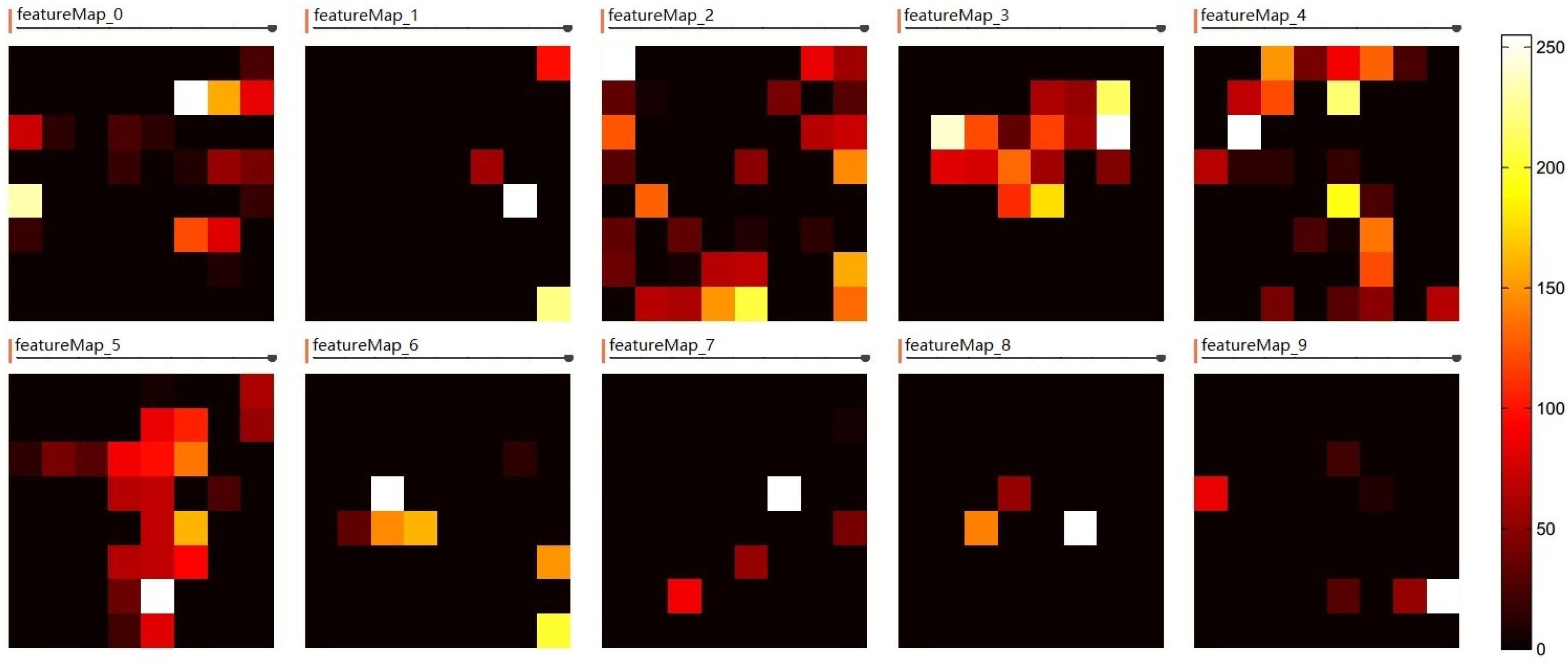
Figure 3 shows ten feature-maps fed into the global pooling layer in DenseNet. As the output size of the last dense block layer is , each feature-map has 64 tiny blocks, and the brighter the feature, the more activation it has. It can be seen from the feature-maps that the features, extracted by previous layers as the input of the global pooling layer, show a kind of sparsity.
Other state-of-the-art CNNs, like ResNet [43], also have the same sparsity feature-maps condition. The reason why feature-maps become sparse lies in the BN [20] and ReLU [21] layers. As the combination of BN and ReLU can achieve favorable feature-extracting performances, more and more CNN structures tend to use BN with ReLU as a common feature normalization and nonlinear transform operator. As shown in Figure 4, the combined operator extracts the most active features from previous feature-maps, which makes the convolution layer more efficient, but inappropriate for global average pool.
The global average pool will dilute the active features when the feature-maps are sparse. That will influence the classification accuracy of the last fully connected layer. Other pooling methods like max pooling [39], stochastic pooling [50] and mixed pooling [51], are seldom used in the global pooling layer, as all have low resistance to noise and low utilization of information when dealing with large scale inputs. To solve this problem, an end-to-end trainable global pool layer has been proposed, named AlphaMEX Global Pool, which has a better trade-off between the average and maximum active features. This structure will learn a better way to pass and extract information through global pooling, which makes the convolutional neural network smarter and more accurate.
3.1.2. AlphaMEX
The original MEX operator has a log-mean-exp function, which has a softmax-like structure [52]:
The input elements are represent by . is the number of input elements. spans a continuum between minimum , average and maximum . The MEX operator has a soft trade-off between minimum and maximum which is controlled by different values of . The function has a “collapsing” property:
where represents the elements of the input matrix, and and represent the number of rows and columns. It is very useful when dealing with CNN feature-map. Another practical property is that the MEX function is differentiable. The partial derivative of and input are given as follows:
The MEX function has desirable properties, but it is hard to initialize or train the parameter , which ranges from 0 to ; indeed, it is impractical to set infinity as the upper limit of the numerical value. Thus, the maximum output from the MEX function is only theoretical. The performance of the function to approximate the maximum output depends on the computing power and base data types of the computer.
To avoid this problem, a novel log-mean-exp function has been proposed, called the AlphaMEX function:
In this continuous function, the trainable parameter ranges from 0 to 1. The AlphaMEX function has more numerical stability and higher efficiency as the following desirable properties:
- Function outputs the minimum value, when right-sided limits to 0:
- Function outputs the average value, when limits to :
- Function outputs the maximum value, when left-sided limits to 1:
- The “collapsing” property:
The trainable parameter can be optimized by any optimizer, such as SGD (Stochastic Gradient Descent) or Adam. The gradient of in back-propagation is calculated as:
In addition, when propagating the gradient from the output to the input of AlphaMEX by the chain rule, the gradient of is given as follows:
Operators and are defined as follows:
Distribution graph of the function is shown in Figure 5.
As shown in Figure 5, the maximum of is less than 0.25 while ranges from 0 to 1. As we hope to output the value between the average and maximum of input in AlphaMEX pooling, the interval of is generally set to (0.5, 1).
3.2. SIFT-Based Movement Calculation
Once the wearer’s location is calculated based on AlphaMEX CNN, the movements of the body are tracked by a novel SIFT matching algorithm, instead of the commonly used inertial sensor. Compared with other related navigation methods, such as optical flow and SLAM (Simultaneous Localization and Mapping), the proposed method neither needs training nor wastes computation for redundant information, such as the movements of single objects or scene reconstruction. The proposed SIFT-based method concentrates on the rotation and translation of the scene plane, which makes the system efficient. The experimental results demonstrate the effectiveness of the algorithm.
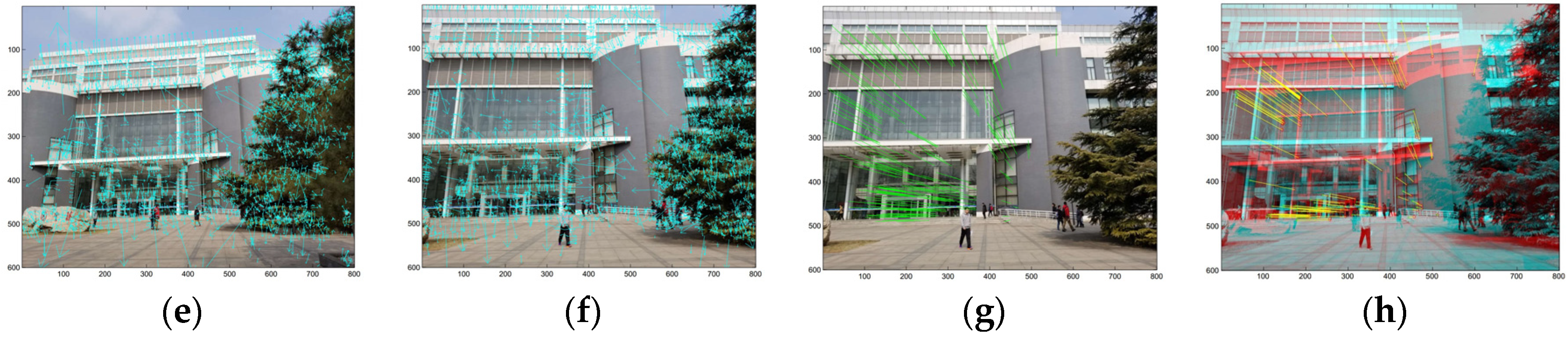
To estimate the wearer’s movement from one frame to the next, SIFT features [19] are extracted for key points in both images, and the matching points between these two images are extracted. The SIFT descriptors for the key points in two frames and the matching results are illustrated in Figure 6. The position changes of the matched key points are then employed to calculate the moving distance or rotation angle between adjacent frames. In this study, the movement of the wearer was limited either to forward movement or rotation, and the size of the location area was assumed to be known to provide a reference for estimating actual distance from the images.
3.2.1. Essential Matrix
To separate different movement types, the essential matrix [53] is employed, which relates corresponding points in stereo images. The essential matrix is defined as:
where is a 3 × 3 rotation matrix representing the orientation of the camera, is a 3-dimensional translation vector, and is the matrix representation of the cross product with .
In addition, for any pair of corresponding points in two images, it satisfies the condition [53]:
The essential matrix can only be used in relation to calibrated cameras since the inner camera parameters must be known in order to achieve the normalization. The camera parameter matrix, , is defined as:
where represents focal length and is referred to as the skew parameter. The number of pixels per unit distance in image coordinates are and , in the and directions, respectively, and are the coordinates of the principal point.
When the cameras are calibrated, the essential matrix can be used for determining both the relative position, , and orientation, , between the cameras. The algorithm is summarized as below:
- Estimate the essential matrix, , by the eight-point algorithm [53], which sets up a least-squares problem with the set of matched SIFT key points.
- Extract and from . Supposing that the Singular-Value Decomposition (SVD) of is , where and are unitary matrices, there are four possible choices for and :where . is defined as:
- Find the correct . Testing with a single point to determine if it is in front of both cameras is sufficient to decide between the four different solutions.
3.2.2. Forward Movement and Rotation of the Camera
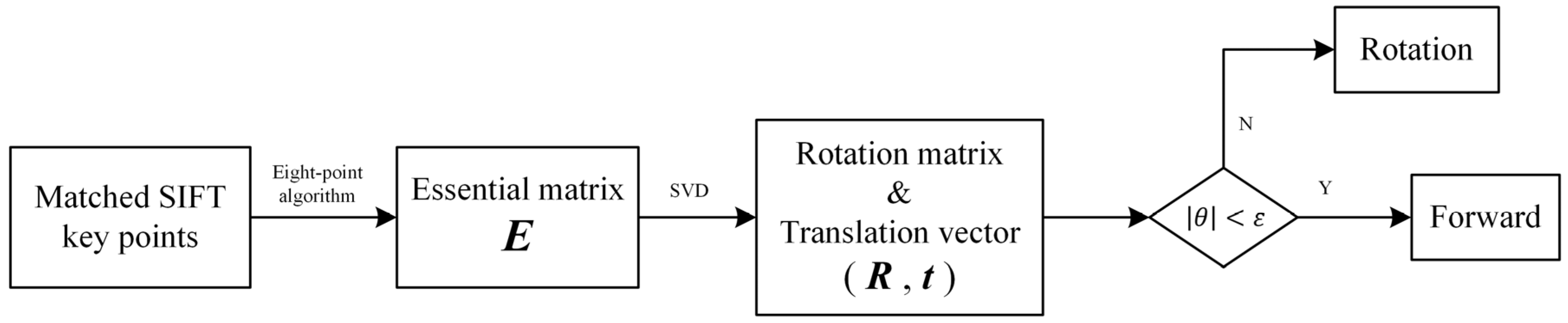
Once the rotation matrix, , is calculated, the rotation angle and rotation axis , where , will be derived. The different movements—moving forward and rotation—are separated by a rotation angle threshold, . Figure 7 shows the data processing flow chart; the essential matrix, , is estimated by eight-point algorithm based on matched SIFT key points. The rotation matrix and translation vector are estimated by SVD. After the judgement block, the movement type will be derived for further calculation.
To estimate the accurate forward movement distance and rotation angle of the wearer, two projection models are built, shown in Figure 8. As the camera is fixed on the chest, yaw and pitch are considered to be the typical rotation types, while roll seldom occurs in walking. Another typical movement is moving forward. As shown in Figure 6, the key points will move in parallel when the camera rotates (yaw or pitch) and move in a radial direction when the camera moves forward. The movements of key points in pixel measurements could be mapped to absolute measurements by the camera parameter matrix, , and the pixel density of the CCD (Charge Coupled Device) in the camera.
In Figure 8a, is the optical center of the camera. represents a key point on scene plane and is the projected point on the CCD (image) plane. When the camera moves forward, toward plane , it is equivalent to moving plane to plane . The original point is denoted as on plane and its projection point is denoted as . is on the extended line of . represents the focal length, , of the camera, so is perpendicular to . According to the similarity between and , the moving distance is presented as follows:
where is the distance between the camera and the reference plane, which is initialized in the first frame and could be estimated iteratively. As there are hundreds of matched key points, the final result is estimated by MLESAC (maximum likelihood estimation sample consensus) [54] algorithm. Similar to Figure 8a, the projection point of is denoted as in the CCD (image) plane in Figure 8b. After the rotation of the camera, the projection point of changes to . As is similar to , is presented as follows:
where is the focal length of the camera. Similarly, is given as follows:
According to the above analysis, the rotation angle can be calculated as:
The final rotation angle is estimated by a fuse function:
3.3. CNN-SIFT Hybrid Pedestrian Navigation
To combined the AlphaMEX CNN-based localization and SIFT-based movement calculation, a novel iterative structure has been designed, as shown in Figure 9.
As the SIFT-based movement estimation requires continuous frames, the iterative structure is appropriate for the hybrid method. Furthermore, in the road detection algorithm (see Section 4.3), an iterative function is indispensable. The proposed iterative structure concisely combines both characteristics. The execution process of the algorithm is described as follows:
- If it is the first frame, feed it into AlphaMEX CNN and output a Road/Scene decision with scene class (if the decision is Scene). If not, name it Frame T, feed it into AlphaMEX CNN and output a Road/Scene decision which is made by both the current frame and the previous frame (see Section 4.3). If the decision is Scene, go to step 2. If not, go to step 3.
- Compare the scene class of the current frame with the scene class of the previous frame. If it is the same, feed these two frames into the SIFT-based movement estimation algorithm and go to step 5. If not, go to step 4.
- Make the global parameter Delay increase one and go to step 1 with next frame. Parameter Delay is used for counting the frames of Road, which is initialized zero and will be initialized after a route is calculated.
- Calculate the distance between the two typical scenes with the product of Delay and the walking speed. The distance helps in drawing routes on the map. Repeat step 1 on next frame.
- Calculate the wearer’s movements and plot the trajectory on the map. Repeat step 1 on next frame.
In this hybrid pedestrian navigation structure, each frame will be firstly analyzed by AlphaMEX CNN for the scene classification, then it will be compared with the previous frame to decide whether the SIFT-based movement calculation should be run. Routes will be calculated by the global parameter Delay if the scene changed. Movements and routes will be plotted on the map for pedestrian navigation.
4. Results
4.1. AlphaMEX CNN Image Classification Results
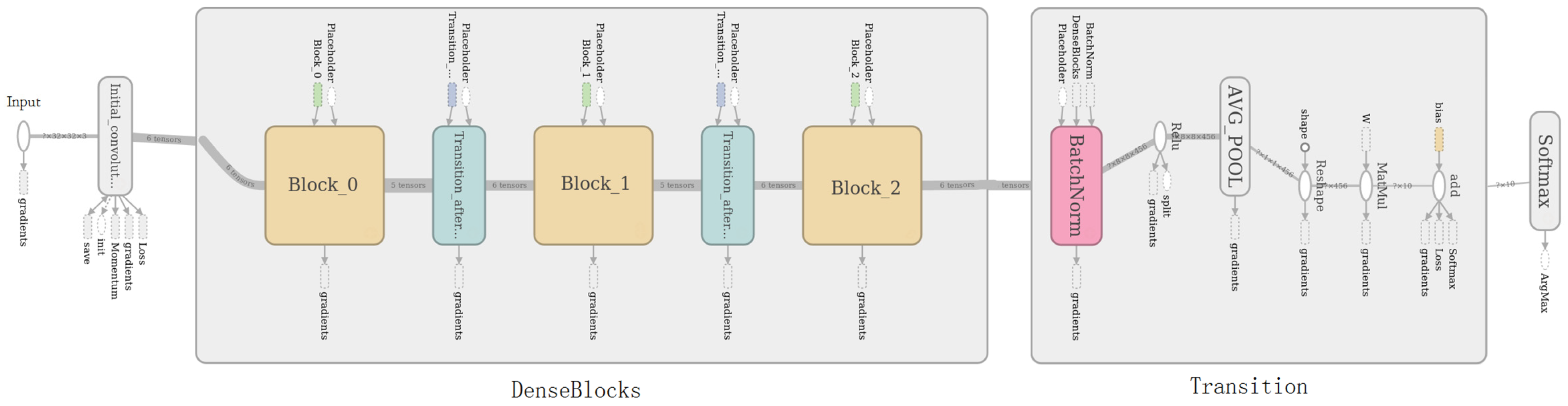
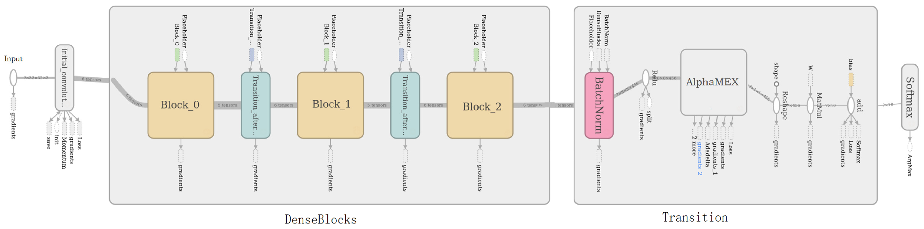
To validate the effectiveness of the proposed AlphaMEX CNN in image classification, the AlphaMEX Global Pool is tested by comparison with DenseNet and other CNN architectures. AlphaMEX Global Pool outperforms the current state-of-the-art results on most benchmark tasks. The DenseNet structure used in our experiments has three dense blocks that each has an equal number of layers (Figure 10). As shown in Figure 2, the original DenseNet40 [44] has a global average pool layer which is performed at the end of the last dense block. The AlphaMEX-DenseNet40 replaces the global average pool by the proposed AlphaMEX Global Pool layer without changing any other layers.
Three benchmark datasets, CIFAR [22], SVHN [23] and ImageNet [24] are used to validate the proposed method. The two CIFAR datasets, CIFAR-10 (C10) and CIFAR-100 (C100), consist of colored natural images with 32 × 32 pixels. CIFAR-10 consists of images drawn from 10 classes and CIFAR-100 from 100 classes. The training and test sets contain 50,000 and 10,000 images, respectively. The SVHN dataset contains 32 × 32 pixel colored digital images. There are 73,257 images in the training set, 26,032 images in the test set. The large-scale dataset, ImageNet, consists of 1.2 million images for training, and 50,000 for validation, from 1000 classes.
Details of DenseNet40 and the proposed AlphaMEX-DenseNet are shown in Table 1. The number of feature-maps increases while images flow through dense blocks. At the end of the last dense block, 456 feature-maps are fed into the global pooling layer, with each sized . In the training stage, the total training epochs are 300, while the initial learning rate is 0.1; decay is 0.1 times at epochs 150 and 225. The batch size is 64 in both training and testing stages and 0.9 momentum [55] is used in momentum optimization. As different parameter initializations will lead the model into different local optimal solutions, three initial values, 0.6, 0.75 and 0.85, have been tested to initialize . The error rates are 5.10%, 5.03% and 5.13%, respectively. All perform better than the original DenseNet40. The initial value of is set to 0.75, which happens to be the median of 0.5 and 1.
Table 1 shows the error rate of the proposed AlphaMEX-DenseNet. It outperforms the original DenseNet (k = 12) by 4.0% on the CIFAR-10 dataset (with standard data augmentation) without adding redundant layers or parameters, which demonstrates the effectiveness of the AlphaMEX Global Pool layer.
In Table 2, state-of-the-art methods (i.e., NIN [41], SimNet [52], All-CNN [56], DSN (Deeply-Supervised Nets) [57], Highway network [42], ResNet [43,58], and DenseNet [44]) are compared to our proposed AlphaMEX Global Pool method on CIFAR-10/CIFAR100 (C10/C100) [22] and SVHN [23]. Standard data augmentation (translation and/or mirroring) is indicated by “+”. The training stage consists of 200 epochs for CIFAR with the initial learning rate 0.1 and 0.1 times decay at epochs 100 and 150, and 40 epochs for SVHN with the same initial learning rate but decay at epochs 20 and 30. The batch size in training is 128, while it is set to 250 in testing. In Table 2, the parameters are given in million, while the top-1 error rate is used. It can be seen that our proposed method achieves competitive classification accuracy.
To further demonstrate the effectiveness of the proposed method on the large-scale dataset, the AlphaMEX structure is tested on ImageNet. The AlphaMEX Global Pool and the global average pool are compared based on the ResNet [43] architecture. The training parameters are set as follows. Training consists of 55 epochs, where the learning rate decreases four times exponentially from 10−2 to 10−4. The batch size in training is 64, while it is set to 512 in testing. Table 3 shows the top-1 error rate and top-5 error rate. AlphaMEX Global Pool outperforms global average pool by 1.7% on top-1 error rate and 1.4% on top-5 error rate. It can be concluded that our proposed method achieves better accuracy on a large-scale dataset.
4.2. SIFT-Based Movement Estimation Results
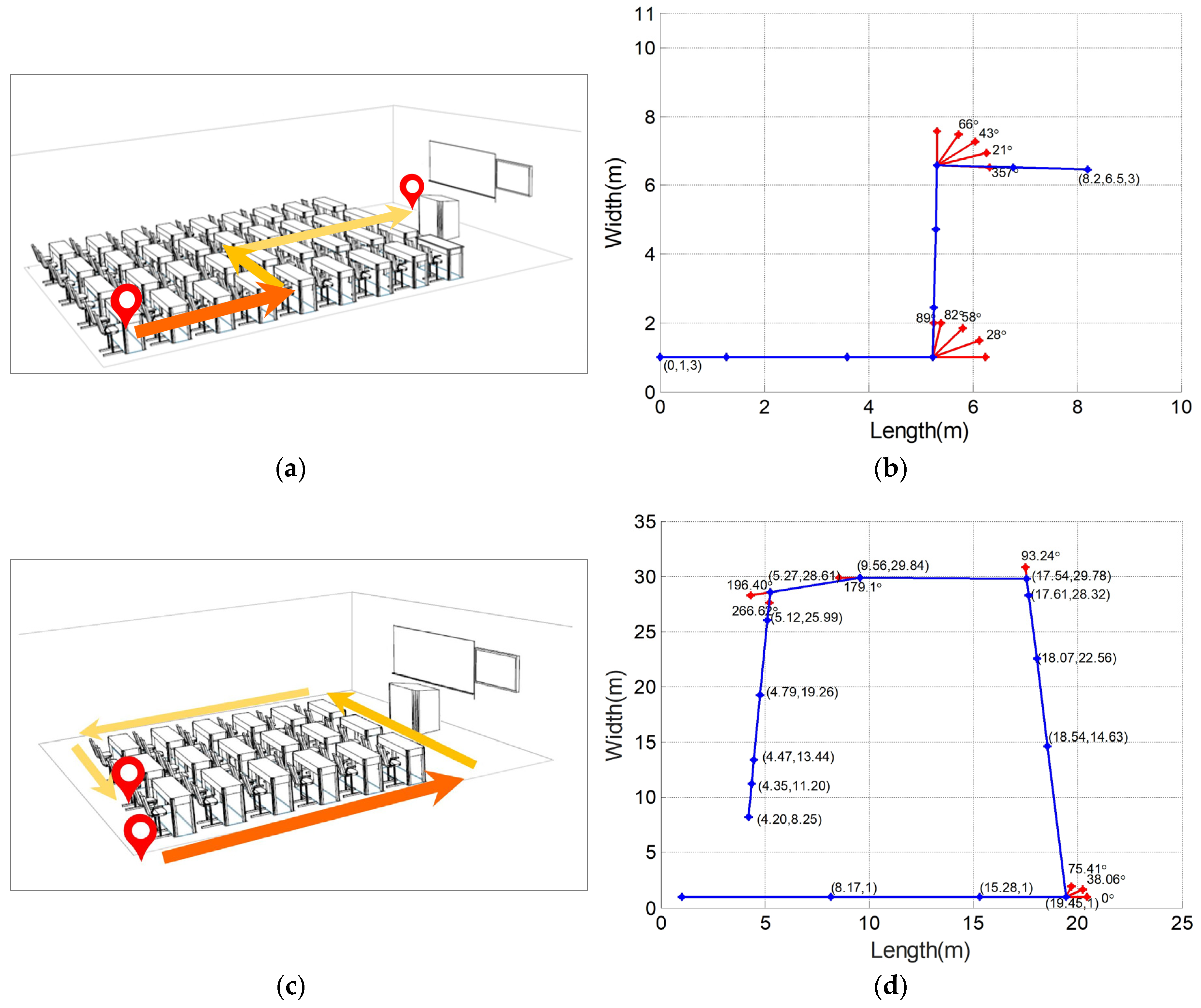
In this section, experiments in a classroom were conducted to validate the accuracy of the proposed SIFT-based movement estimation method. The width and length of the classroom were 11 m and 10 m, respectively. The initial position of the wearer in relation to the walls was assumed to be a priori knowledge. A route was designed to include three segments of walking forward, and two segments of 90 rotation. Images were acquired by a wearable camera at pre-set locations, as well as during rotation. The focal length of the camera was 4.2 mm. was set to 0.9. A total of 17 full-resolution images were obtained, and downsampled to 816 × 612 pixels by bilinear interpolation for further analysis. In the experiments, MLESAC was employed to remove the outliers. Camera motion stabilization [59] was used to remove undesired motions of the camera. The corresponding location/orientation was then computed based on the essential matrix between adjacent images. In the experiments, SIFT and the camera motion stabilization algorithm were realized by OpenCV (Open Source Computer Vision Library) while the MLESAC algorithm is realized follow the structure in [54].
After calculating the moving distance and rotation angle each time the camera moved, the trajectory of the camera was plotted and compared with the pre-defined route, as shown in Figure 11. In Figure 11b,d, the straight lines represent the moving track. The “*” points on the straight lines represent the camera location where each image was taken while the “*” points near the corner represent the camera orientation.
Table 4 and Table 5 show the calculated moving distance and rotation angle corresponding to each image. The comparison with the actual distance and rotation angle is also listed. The average absolute error of moving distance estimation is 0.52 m with 0.41 standard deviation. The average absolute error of rotation angle is 2.66° with 1.26° standard deviation. It can be seen that the movements can be estimated with an adequate accuracy.
4.3. Pedestrian Navigation Results
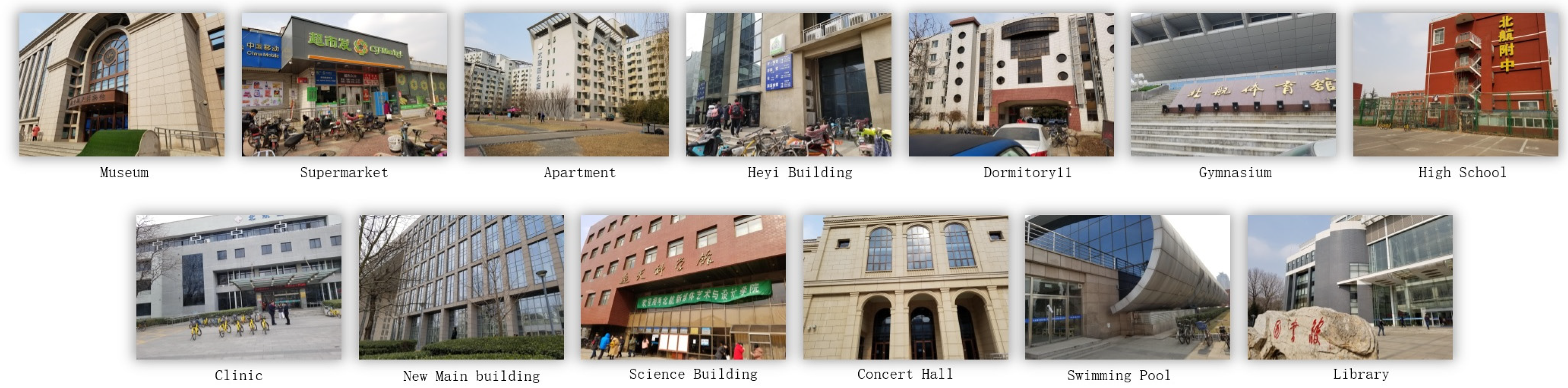
To further validate the proposed FPV pedestrian navigation system, a high-resolution FPV dataset was built, as shown in Figure 12. It has 13 typical scenes (i.e., museum, apartment, clinic, gymnasium, etc.) from BUAA (Beijing University of Aeronautics and Astronautics) with 4032 × 3024 sRGB resolution. Each scene class has 200 images from different shooting angles.
An AlphaMEX-ResNet was trained on the BuaaFPV dataset with the proposed AlphaMEX Global Pool and four ResBlocks, as shown in Figure 1. To estimate the location area more effectively, the AlphaMEX-ResNet was trained for 55 epochs with 224 × 224 crop size. The test result reached 95% in accuracy, while the original ResNet reached 94% with the same training condition.
The sensor used in the experiments was an MI5100, which has 1/2.5 inch (4:3) sensor size, 2.2 pixel size, and 5.7 mm × 4.28 mm image area. The focal length of the camera was 16 mm. The camera is connected with the server by 4 G cellular network. In the server, a single GTX1080Ti GPU was installed with a i7-7700K CPU and 16 GB memory for calculations.
Figure 13 and Figure 14 show parts of the location estimation results in the real-time test. The camera was fixed on the chest of the human body and taking FPV images with 1.5 Hz shooting frequency. Once it received a new sequential FPV image, the AlphaMEX-ResNet estimated the confidence of each scene class within 3.87 ms. Figure 13 shows the location estimation result from “Apartment” to “High School”; each dot in the chart represents the confidence of each frame with different colors representing scene classes as shown in the legend. A total of 145 frames were estimated in this clip, with the horizontal ordinate representing the timeline. In the real-time test, as the wearer walked through each typical scene area, roads became another “scene”, which appeared with high frequency. In this experiment, the large number of unpredictable objects flashing into the scene when the wearer walked by the road (such as cars, people, bicycles, etc.), were treated as a kind of noise when dealing with the special scene “road”. As shown in Figure 13 and Figure 14, when the wearer walked in a typical scene area, the algorithm demonstrated the absolute confidence of its estimation, but reflected this noise when the wearer walked by the road, as we expected.
According to the above analysis, three rules have been made to improve the location estimation accuracy:
- Frames with continuous absolute confidence are accepted as a typical scene.
- If the maximum confidence of a frame or its previous frame is lower than 0.85, it will be identified as “Road”.
- As the wearer walks with constant speed (1.4m/s), the period represents the walking distance.
The absolute confidence threshold, 0.85, is an empirical parameter determined by testing in a large number of experiments. It is used to determine whether the algorithm has absolute confidence with its classification of each frame. To reduce the influence of noise, the system does not test the current frame only, but also the previous frame, as described in the second rule. The reason for this is that a person is not able to change places and come back in a very short time. Thus, this method could filter the peaks caused by noise. This strategy maintains the accuracy of the scene classification.
In the experiment, the proposed SIFT-based movement estimation and tracking algorithm is validated on an FPV clip of “Apartment”, as shown in Figure 15. It can be seen that the test clip has several “moving forward” and “rotation” movements, and the whole trajectory resembles a “U” shape.
The location of the first frame in relation to the scene plane is assumed to be a priori knowledge stored in the database and is set to 10°. The system reaches 0.18 s/frame in the experiments. The final FPV-based pedestrian navigation result is shown in Figure 16; Figure 16a shows the movement estimation and tracking result, and Figure 16b plots the scene recognition result with a route estimation. The navigation algorithm has an average absolute error of 0.57 m in distance estimation at each checkpoint. As shown in the image, both the position and movements can be well estimated by the proposed pedestrian navigation algorithm using a single wearable camera.
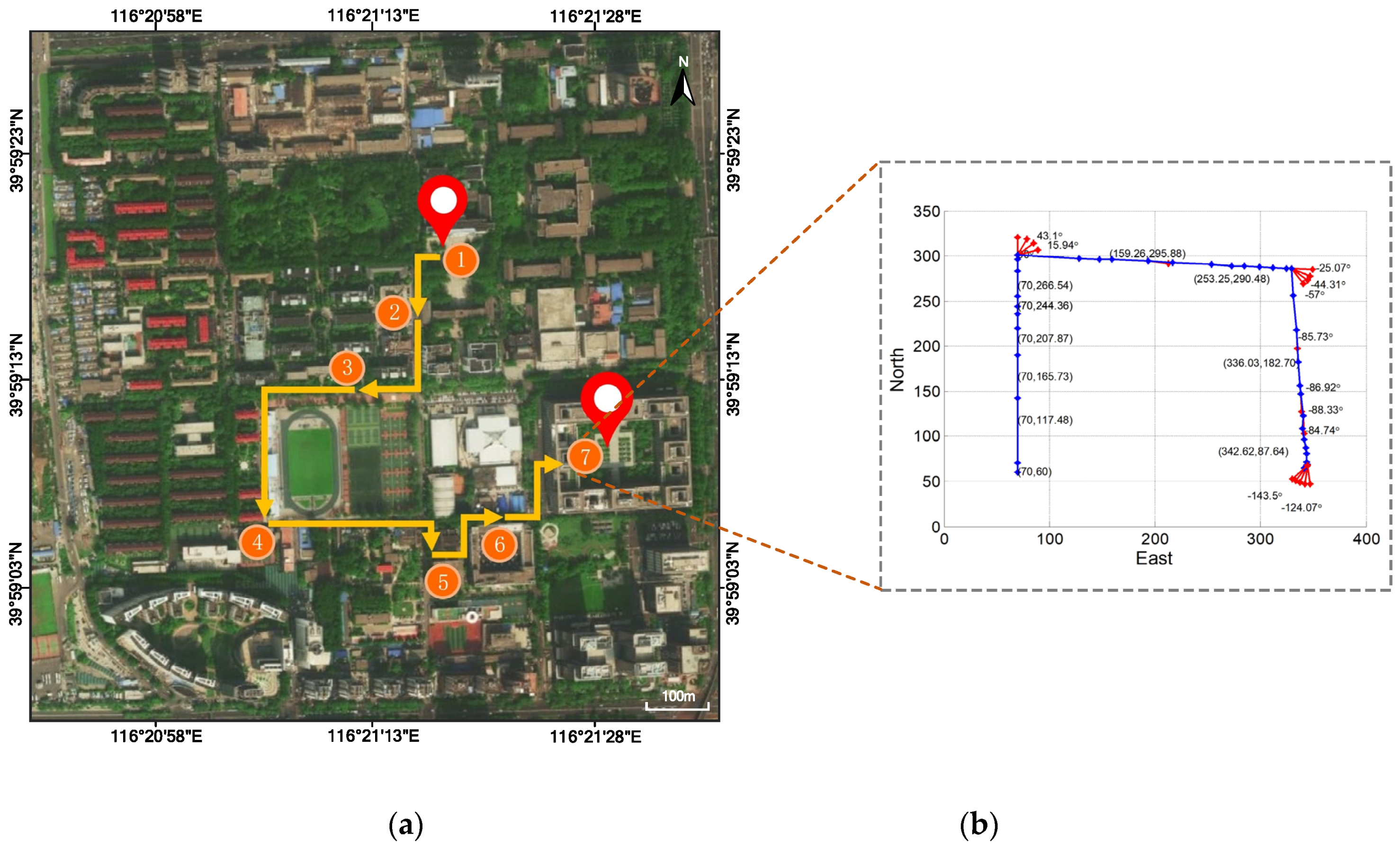
To further validate the expansibility of the proposed method, more typical scenes were added to BuaaFPV dataset, including the Zhixing Building, the Engineering Training Building and the Institute of UAV (Unmanned Aerial Vehicle). Thus the new BuaaFPV dataset was expanded to 16 typical scenes with 4032 × 3024 sRGB resolution. The AlphaMEX CNN model was retrained based on the new dataset. Figure 17 shows the pedestrian navigation result, which demonstrates the expansibility of the hybrid pedestrian navigation method. Figure 17a plots the scene recognition result with a route estimation, and Figure 17b shows the movement estimation and tracking result.
5. Discussion
The proposed FPV-based pedestrian navigation system is generally useful, and necessary in areas where GPS or other radio-wave strength methods are blocked; this is especially true for visually impaired people, who require a localization method that can work in any urban area, ranging from underground to narrow open-sky pavements enclosed by tall buildings. The proposed AlphaMEX based-CNN, which could be well trained end-to-end, outperforms the state-of-the-art CNN structures in scene classification. The top-1 error rate of the proposed AlphaMEX-ResNet outperforms the original ResNet (k = 12) by 1.7% on the ImageNet dataset. To combine the AlphaMEX CNN-based localization and SIFT-based movement estimation, a novel iterative structure was designed. The whole pedestrian navigation system was 0.18 s/frame in the experiments. The average absolute error of the CNN-SIFT hybrid pedestrian navigation system was 0.57 m, which is an adequate accuracy for pedestrian navigation. The routes and movements can be plotted on the map for pedestrian navigation.
However, the proposed algorithm also has some limitations. First, as the absolute measurement was estimated by the essential matrix and the camera parameters, the numerical calculation error limited the accuracy of the system. A trainable distance estimation algorithm based on machine learning could help to further improve the estimation. Second, two typical movements, moving forward and rotation, are analyzed in the algorithm. More types of movements, such as walking up stairs, could be analyzed by similar methods to enhance navigation with out-of-plane motion. Finally, the system is designed for pedestrian navigation under good weather conditions, and more image preprocessing algorithms could help to deal with bad weather and low illumination conditions.
6. Conclusions
In this paper, we introduced a hybrid structure with CNN and local image features SIFT for pedestrian navigation based on FPV. A novel end-to-end trainable global pooling operator, called AlphaMEX, was designed to improve the scene classification accuracy of CNN. In addition, a SIFT-based tracking algorithm was employed to calculate the movement of a person and track their trajectory through each frame of FPV. Experimental results demonstrate the effectiveness of the proposed method. The AlphaMEX Global Pool method achieves competitive accuracy and outperforms original state-of-the-art methods. The top-1 error rate of the proposed AlphaMEX-ResNet outperforms the original ResNet (k = 12) by 1.7% on the ImageNet dataset. The average absolute error of the CNN-SIFT hybrid pedestrian navigation system is 0.57 m, which is an adequate accuracy for pedestrian navigation. Both position and movement can be well estimated by the proposed hybrid pedestrian navigation algorithm with a single wearable camera.
Author Contributions
Conceptualization, Q.Z.; Methodology, Q.Z. and B.Z.; Resources, B.Z., D.S. and W.F.; Software, S.L.; Writing—original draft, H.Z. and G.L.
Funding
Please add: This research was funded by the National Natural Science Foundation of China grant number 61772052.
Acknowledgments
The authors would like to acknowledge the School of Electronics and Information Engineering, Beihang University, and the Image Processing Center of Beihang University for the continuous support in our research activity.
Conflicts of Interest
The authors declare no conflict of interest.
References
- Betancourt, A.; Morerio, P.; Regazzoni, C.S.; Rauterberg, M. The evolution of First-Person Vision methods: A survey. IEEE Trans. Circuits Syst. Video Technol. 2015, 25, 744–760. [Google Scholar] [CrossRef]
- Kanade, T.; Hebert, M. First-person vision. Proc. IEEE 2012, 100, 2442–2453. [Google Scholar] [CrossRef]
- Li, C.; Kitani, K.M. Model recommendation with virtual probes for egocentric hand detection. In Proceedings of the 2013 IEEE International Conference on Computer Vision (ICCV), Sydney, Australia, 1–8 December 2013; pp. 2624–2631. [Google Scholar]
- Li, C.; Kitani, K.M. Pixel-level hand detection in ego-centric videos. In Proceedings of the IEEE Computer Vision and Pattern Recognition (CVPR), Orlando, FL, USA, 23–28 June 2013; pp. 3570–3577. [Google Scholar]
- Wang, H.; Choudhury, R.R.; Nelakuditi, S.; Bao, X. InSight: Recognizing humans without face recognition. In Proceedings of the 14th Workshop on Mobile Computing Systems and Applications, Jekyll Island, GA, USA, 26–27 February 2013; p. 7. [Google Scholar]
- Zariffa, J.; Popovic, M.R. Hand contour detection in wearable camera video using an adaptive histogram region of interest. J. Neuroeng. Rehabilit. 2013, 10, 114. [Google Scholar] [CrossRef] [PubMed] [Green Version]
- Narayan, S.; Kankanhalli, M.S.; Ramakrishnan, K.R. Action and interaction recognition in first-person videos. In Proceedings of the IEEE Conference on Computer Vision and Pattern Recognition Workshops, Columbus, OH, USA, 23–28 June 2014; pp. 526–532. [Google Scholar]
- Matsuo, K.; Yamada, K.; Ueno, S.; Naito, S. An attention-based activity recognition for egocentric video. In Proceedings of the 2014 IEEE Conference on Computer Vision and Pattern Recognition Workshops (CVPRW), Columbus, OH, USA, 23–28 June 2014; pp. 565–570. [Google Scholar]
- Damen, D.; Leelasawassuk, T.; Haines, O.; Calway, A.; Mayol-Cuevas, W. Multi-user egocentric online system for unsupervised assistance on object usage. In Proceedings of the European Conference on Computer Vision, Zurich, Switzerland, 6–7 September 2014; pp. 481–492. [Google Scholar]
- Poleg, Y.; Arora, C.; Peleg, S. Temporal segmentation of egocentric videos. In Proceedings of the IEEE Conference on Computer Vision and Pattern Recognition (CVPR), Columbus, OH, USA, 23–28 June 2014; pp. 2537–2544. [Google Scholar]
- Zheng, K.; Lin, Y.; Zhou, Y.; Salvi, D.; Fan, X.; Guo, D.; Wang, S. Video-based action detection using multiple wearable cameras. In Proceedings of the European Conference on Computer Vision, Zurich, Switzerland, 6–7 September 2014; pp. 727–741. [Google Scholar]
- Castle, R.O.; Gawley, D.J.; Klein, G.; Murray, D.W. Video-rate recognition and localization for wearable cameras. In Proceedings of the British Machine Vision Conference, Coventry, UK, 10–13 September 2007; pp. 1–10. [Google Scholar]
- Castle, R.O.; Gawley, D.J.; Klein, G.; Murray, D.W. Towards simultaneous recognition, localization and mapping for hand-held and wearable cameras. In Proceedings of the 2007 IEEE International Conference on Robotics and Automation, Roma, Italy, 10–14 April 2007; pp. 4102–4107. [Google Scholar]
- Davison, A.J.; Reid, I.D.; Molton, N.D.; Stasse, O. MonoSLAM: Real-time single camera SLAM. IEEE Trans. Pattern Anal. Mach. Intell. 2007, 29, 1052–1067. [Google Scholar] [CrossRef] [PubMed] [Green Version]
- Castle, R.; Klein, G.; Murray, D.W. Video-rate localization in multiple maps for wearable augmented reality. In Proceedings of the 12th IEEE International Symposium on Wearable Computers (ISWC), Pittsburgh, PA, USA, 28 September–1 October 2008; pp. 15–22. [Google Scholar]
- Kameda, Y.; Ohta, Y. Image retrieval of First-Person Vision for pedestrian navigation in urban area. In Proceedings of the 2010 20th International Conference on Pattern Recognition (ICPR), Istanbul, Turkey, 23–26 August 2010; pp. 364–367. [Google Scholar]
- Li, T.; Zhang, H.; Gao, Z.; Chen, Q.; Niu, X. High-Accuracy Positioning in Urban Environments Using Single-Frequency Multi-GNSS RTK/MEMS-IMU Integration. Remote Sens. 2018, 10, 205. [Google Scholar] [CrossRef]
- Krizhevsky, A.; Sutskever, I.; Hinton, G.E. ImageNet classification with deep convolutional neural networks. Adv. Neural Inf. Process. Syst. 2012, 25, 1097–1105. [Google Scholar] [CrossRef]
- Lowe, D.G. Object recognition from local scale-invariant features. In Proceedings of the Seventh IEEE International Conference on Computer Vision, Kerkyra, Greece, 20–27 September 1999; pp. 1150–1157. [Google Scholar]
- Ioffe, S.; Szegedy, C. Batch normalization: Accelerating deep network training by reducing internal covariate shift. In Proceedings of the International Conference on Machine Learning, Lille, France, 6–11 July 2015; pp. 448–456. [Google Scholar]
- Glorot, X.; Bordes, A.; Bengio, Y. Deep sparse rectifier neural networks. In Proceedings of the Fourteenth International Conference on Artificial Intelligence and Statistics, Ft. Lauderdale, FL, USA, 11–13 April 2011; pp. 315–323. [Google Scholar]
- Krizhevsky, A.; Hinton, G. Learning Multiple Layers of Features from Tiny Images. Tech Report. 2009. Available online: http://citeseerx.ist.psu.edu/viewdoc/download?doi=10.1.1.222.9220&rep=rep1&type=pdf (accessed on 8 April 2009).
- Netzer, Y.; Wang, T.; Coates, A.; Bissacco, A.; Wu, B.; Ng, A.Y. Reading digits in natural images with unsupervised feature learning. In Proceedings of the Advances in Neural Information Processing Systems Workshop on Deep Learning and Unsupervised Feature Learning, Granada, Spain, 12–17 December 2011; p. 5. [Google Scholar]
- Deng, J.; Dong, W.; Socher, R.; Li, L.; Li, K.; Fei-Fei, L. Imagenet: A large-scale hierarchical image database. In Proceedings of the IEEE Conference on Computer Visual Pattern Recognition, Miami, FL, USA, 20–25 June 2009; pp. 248–255. [Google Scholar]
- Fathi, A.; Hodgins, J.K.; Rehg, J.M. Social interactions: A first-person perspective. In Proceedings of the 2012 IEEE Conference on Computer Vision and Pattern Recognition, Providence, RI, USA, 16–21 June 2012; pp. 1226–1233. [Google Scholar]
- Yarbus, A.L. Eye movements during perception of complex objects. In Eye Movements and Vision; Springer: Boston, MA, USA, 1967; pp. 171–211. [Google Scholar]
- Bisio, I.; Delfino, A.; Lavagetto, F.; Marchese, M. Opportunistic detection methods for emotion-aware smartphone applications. In Psychology and Mental Health: Concepts, Methodologies, Tools, and Applications; IGI Global: Hershey, PA, USA, 2016; pp. 670–704. [Google Scholar]
- Philipose, M.; Ren, X. Egocentric recognition of handled objects: Benchmark and analysis. In Proceedings of the 2009 IEEE Computer Society Conference on Computer Vision and Pattern Recognition Workshops, Miami, FL, USA, 20–25 June 2009; pp. 1–8. [Google Scholar]
- Betancourt, A.; López, M.M.; Regazzoni, C.S.; Rauterberg, M. A sequential classifier for hand detection in the framework of egocentric vision. In Proceedings of the IEEE Conference on Computer Vision and Pattern Recognition (CVPR) Workshops, Columbus, OH, USA, 23–28 June 2014; pp. 600–605. [Google Scholar]
- Lu, Z.; Grauman, K. Story-driven summarization for egocentric video. In Proceedings of the IEEE Conference on Computer Vision and Pattern Recognition, Portland, OR, USA, 23–28 June 2013; pp. 2714–2721. [Google Scholar]
- Hodges, S.; Williams, L.; Berry, E.; Izadi, S.; Srinivasan, J.; Butler, A.; Wood, K. SenseCam: A retrospective memory aid. In Proceedings of the International Conference on Ubiquitous Computing, Orange County, CA, USA, 17–21 September 2006; pp. 177–193. [Google Scholar]
- Sundaram, S.; Cuevas, W.W.M. High level activity recognition using low resolution wearable vision. In Proceedings of the 2009 IEEE Computer Society Conference on Computer Vision and Pattern Recognition Workshops, Miami, FL, USA, 20–25 June 2009; pp. 25–32. [Google Scholar]
- Ogaki, K.; Kitani, K.M.; Sugano, Y.; Sato, Y. Coupling eye-motion and ego-motion features for first-person activity recognition. In Proceedings of the 2012 IEEE Computer Society Conference on Computer Vision and Pattern Recognition Workshops, Providence, RI, USA, 16–21 June 2012; pp. 1–7. [Google Scholar]
- He, K.; Gkioxari, G.; Dollár, P.; Girshick, R. Mask r-cnn. In Proceedings of the IEEE International Conference on Computer Vision (ICCV), Venice, Italy, 22–29 October 2017; pp. 2980–2988. [Google Scholar]
- Takizawa, H.; Orita, K.; Aoyagi, M.; Ezaki, N.; Mizuno, S. A Spot Navigation System for the Visually Impaired by Use of SIFT-Based Image Matching. In Proceedings of the International Conference on Universal Access in Human-Computer Interaction, Los Angeles, CA, USA, 2–7 August 2015; pp. 160–167. [Google Scholar]
- Hu, M.; Chen, J.; Shi, C. Three-dimensional mapping based on SIFT and RANSAC for mobile robot. In Proceedings of the 2015 IEEE International Conference on Cyber Technology in Automation, Control, and Intelligent Systems (CYBER), Shenyang, China, 8–12 June 2015; pp. 139–144. [Google Scholar]
- Pang, Y.; Sun, M.; Jiang, X.; Li, X. Convolution in convolution for network in network. IEEE Trans. Neural Netw. Learn. Syst. 2017, 29, 1587–1597. [Google Scholar] [CrossRef] [PubMed]
- Zhang, D.; Han, J.; Han, J.; Shao, L. Cosaliency detection based on intrasaliency prior transfer and deep intersaliency mining. IEEE Trans. Neural Netw. Learn. Syst. 2016, 27, 1163–1176. [Google Scholar] [CrossRef] [PubMed]
- Kim, Y. Convolutional neural networks for sentence classification. arXiv, 2014; arXiv:1408.5882. [Google Scholar]
- LeCun, Y.; Bottou, L.; Bengio, Y.; Haffner, P. Gradient-based learning applied to document recognition. Proc. IEEE 1998, 86, 2278–2324. [Google Scholar] [CrossRef] [Green Version]
- Lin, M.; Chen, Q.; Yan, S. Network in network. arXiv, 2013; arXiv:1312.4400. [Google Scholar]
- Srivastava, R.K.; Greff, K.; Schmidhuber, J. Training very deep networks. In Proceedings of the Twenty-ninth Annual Conference on Neural Information Processing Systems, Montreal, QC, Canada, 7–12 December 2015; pp. 2377–2385. [Google Scholar]
- He, K.; Zhang, X.; Ren, S.; Sun, J. Deep residual learning for image recognition. In Proceedings of the IEEE Conference on Computer Visual Pattern Recognition, Las Vegas, NV, USA, 27–30 June 2016; pp. 770–778. [Google Scholar]
- Huang, G.; Liu, Z.; Weinberger, K.Q.; Maaten, L. Densely connected convolutional networks. In Proceedings of the IEEE Conference on Computer Vision and Pattern Recognition, Honolulu, HI, USA, 21–26 July 2017; p. 3. [Google Scholar]
- Khoshkbarforoushha, A.; Khosravian, A.; Ranjan, R. Elasticity management of streaming data analytics flows on clouds. J. Comput. Syst. Sci. 2017, 89, 24–40. [Google Scholar] [CrossRef]
- Khoshkbarforoushha, A.; Ranjan, R.; Gaire, R.; Abbasnejad, E.; Wang, L. Distribution based workload modelling of continuous queries in clouds. IEEE Trans. Emerg. Top. Comput. 2017, 5, 120–133. [Google Scholar] [CrossRef]
- Ma, Y.; Wang, L.; Zomaya, A.Y.; Chen, D.; Ranjan, R. Task-tree based large-scale mosaicking for massive remote sensed imageries with dynamic dag scheduling. IEEE Trans. Parallel Distrib. Syst. 2014, 25, 2126–2137. [Google Scholar] [CrossRef]
- Wang, L.; Ma, Y.; Zomaya, A.Y.; Ranjan, R.; Chen, D. A parallel file system with application-aware data layout policies for massive remote sensing image processing in digital earth. IEEE Trans. Parallel Distrib. Syst. 2015, 26, 1497–1508. [Google Scholar] [CrossRef]
- Menzel, M.; Ranjan, R.; Wang, L.; Khan, S.U.; Chen, J. CloudGenius: A hybrid decision support method for automating the migration of web application clusters to public clouds. IEEE Trans. Comput. 2015, 64, 1336–1348. [Google Scholar] [CrossRef]
- Zeiler, M.D.; Fergus, R. Stochastic pooling for regularization of deep convolutional neural networks. arXiv, 2013; arXiv:1301.3557. [Google Scholar]
- Lee, C.Y.; Gallagher, P.W.; Tu, Z. Generalizing pooling functions in convolutional neural networks: Mixed, gated, and tree. In Proceedings of the 19th International Conference on Artificial Intelligence and Statistics (AISTATS), Cadiz, Spain, 7–11 May 2016; pp. 464–472. [Google Scholar]
- Cohen, N.; Sharir, O.; Shashua, A. Deep simnets. In Proceedings of the IEEE Conference on Computer Vision and Pattern Recognition, Las Vegas, NV, USA, 27–30 June 2016; pp. 4782–4791. [Google Scholar]
- Hartley, R.; Zisserman, A. Multiple View Geometry in Computer Vision; Cambridge University Press: Cambridge, UK, 2003; pp. 237–360. [Google Scholar]
- Torr, P.H.; Zisserman, A. MLESAC: A new robust estimator with application to estimating image geometry. Comput. Vis. Image Underst. 2000, 78, 138–156. [Google Scholar] [CrossRef]
- Sutskever, I.; Martens, J.; Dahl, G.; Hinton, G. On the importance of initialization and momentum in deep learning. In Proceedings of the 30th International Conference on Machine Learning, Atlanta, GA, USA, 16–21 June 2013; pp. 1139–1147. [Google Scholar]
- Springenberg, J.T.; Dosovitskiy, A.; Brox, T.; Riedmiller, M. Striving for simplicity: The all convolutional net. arXiv, 2014; arXiv:1412.6806. [Google Scholar]
- Lee, C.Y.; Xie, S.; Gallagher, P.; Zhang, Z.; Tu, Z. Deeply-supervised nets. In Proceedings of the Eighteenth International Conference on Artificial Intelligence and Statistics, San Diego, CA, USA, 10–12 May 2015; pp. 562–570. [Google Scholar]
- Huang, G.; Sun, Y.; Liu, Z.; Sedra, D.; Weinberger, K.Q. Deep networks with stochastic depth. In Proceedings of the European Conference on Computer Vision, Amsterdam, The Netherlands, 11–14 October 2016; pp. 646–661. [Google Scholar]
- Matsushita, Y.; Ofek, E.; Ge, W.; Tang, X.; Shum, H.Y. Full-frame video stabilization with motion inpainting. IEEE Trans. Pattern Anal. Mach. Intell. 2006, 28, 1150–1163. [Google Scholar] [CrossRef] [PubMed]
Figure 1.
Flow diagram of the proposed FPV (first-person vision) pedestrian navigation algorithm. Solid blue lines represent the flow of sequence frames, whereas solid yellow lines represent the flow of internal functions.
Figure 1.
Flow diagram of the proposed FPV (first-person vision) pedestrian navigation algorithm. Solid blue lines represent the flow of sequence frames, whereas solid yellow lines represent the flow of internal functions.
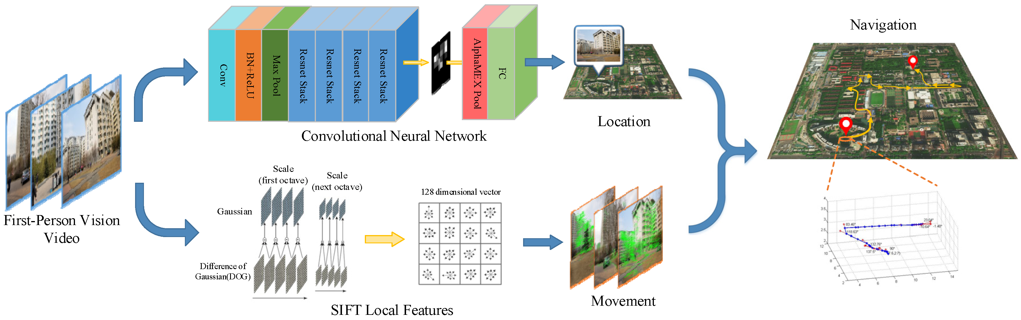
Figure 2.
DenseNet-40 (DenseNet with 40 layers) architecture for CIFAR with three dense blocks and a global average pool layer. The squares in DenseBlocks represent the three dense blocks. The rounded rectangle with the label AVG_POOL in Transition represents the global average pool layer.
Figure 2.
DenseNet-40 (DenseNet with 40 layers) architecture for CIFAR with three dense blocks and a global average pool layer. The squares in DenseBlocks represent the three dense blocks. The rounded rectangle with the label AVG_POOL in Transition represents the global average pool layer.

Figure 3.
Feature-maps fed into the global average pool in DenseNet. Each feature-map has 64 tiny blocks (features); the brighter the block, more activation the feature has. The feature-maps show a kind of sparsity.
Figure 3.
Feature-maps fed into the global average pool in DenseNet. Each feature-map has 64 tiny blocks (features); the brighter the block, more activation the feature has. The feature-maps show a kind of sparsity.

Figure 4.
Sketch map of feature extraction by batch normalization (BN) and rectified linear unit (ReLU). The combined operator will extract the most active features from previous feature-maps, which makes the convolution layer more efficient, but also makes the feature-map sparse.
Figure 4.
Sketch map of feature extraction by batch normalization (BN) and rectified linear unit (ReLU). The combined operator will extract the most active features from previous feature-maps, which makes the convolution layer more efficient, but also makes the feature-map sparse.
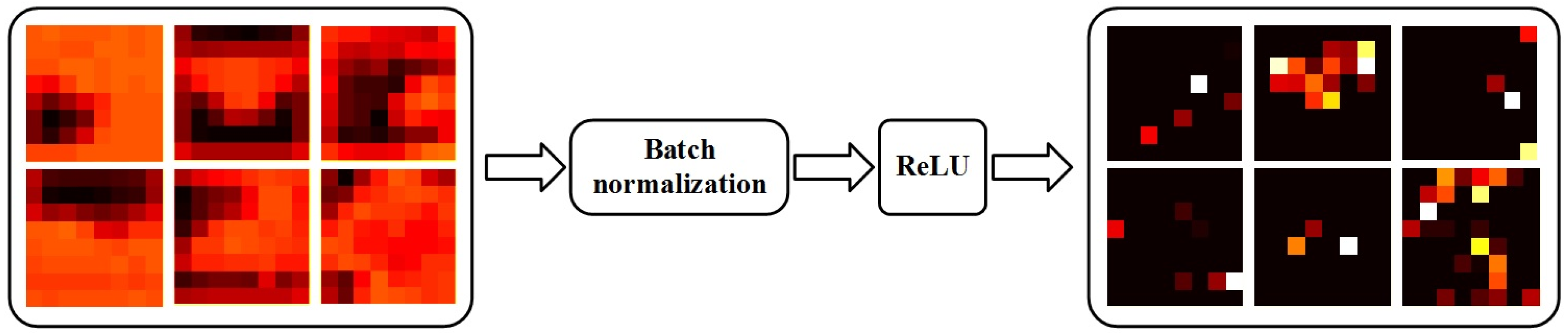
Figure 5.
Distribution graph of function. The extremum of Γ(α) is less than 0.25, while α ranges from 0 to 1. The interval of α is generally set (0.5, 1) in the AlphaMEX Global Pool.
Figure 5.
Distribution graph of function. The extremum of Γ(α) is less than 0.25, while α ranges from 0 to 1. The interval of α is generally set (0.5, 1) in the AlphaMEX Global Pool.
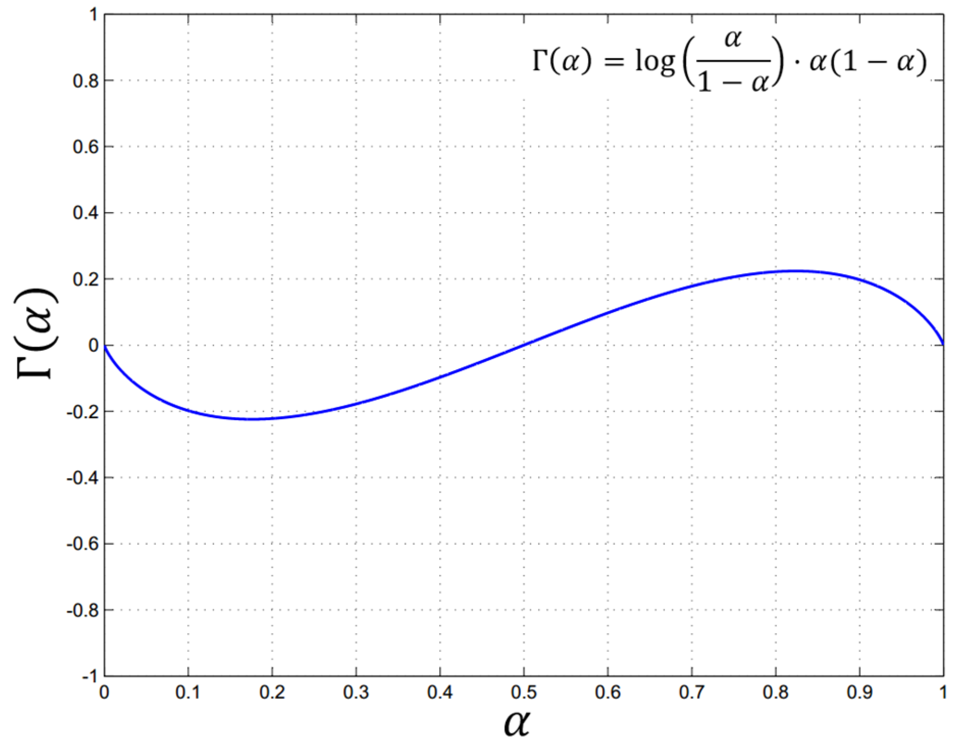
Figure 6.
Matching of scale-invariant feature transform (SIFT) descriptor. (a,b) Two adjacent images with SIFT features corresponding to a rotation of the camera; (c) displacement of the key points from (a) to (b); (d) inliers to compute the essential matrix; (e,f) two adjacent images with SIFT features corresponding to a forward movement of the camera; (g) displacement of the key points from (e) to (f); (h) inliers to compute the essential matrix. By observing the position change of the key points from one frame to the next, key points move in a radial direction when the camera moves forward and move in parallel when the camera rotates.
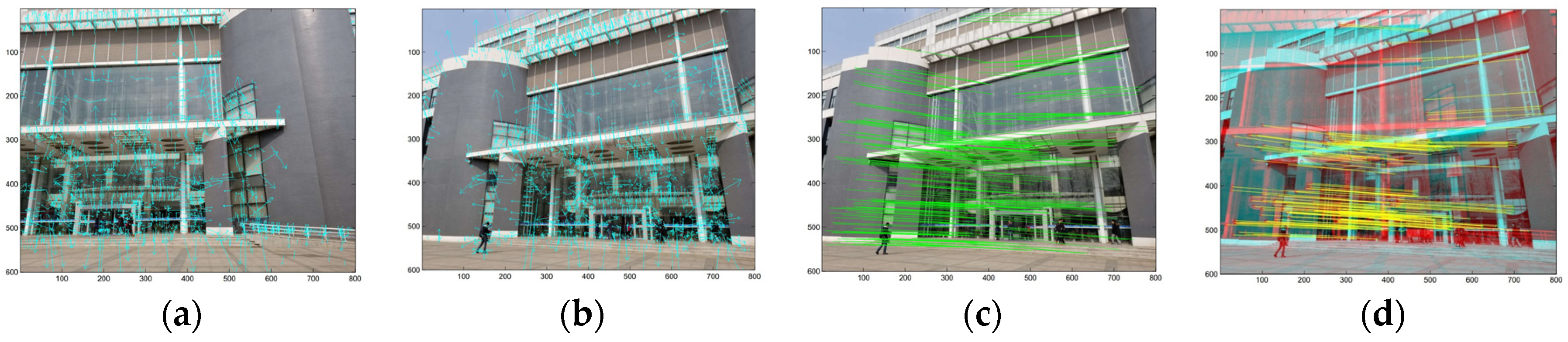

Figure 7.
Flow chart of movement estimation based on SIFT. The essential matrix, E, is estimated by eight-point algorithm based on matched SIFT key points. The rotation matrix, , and translation vector, , are estimated by SVD. The movement type will be derived through the judgement block with the rotation angle, , and angle threshold, .

Figure 8.
Projection models of the camera. is the optical center of the camera. represents a key point on scene plane and is the projected point on the CCD (image) plane. is the focal length. (a) Camera moves forward, is the moving distance; (b) camera rotates, is the rotation angle.
Figure 8.
Projection models of the camera. is the optical center of the camera. represents a key point on scene plane and is the projected point on the CCD (image) plane. is the focal length. (a) Camera moves forward, is the moving distance; (b) camera rotates, is the rotation angle.
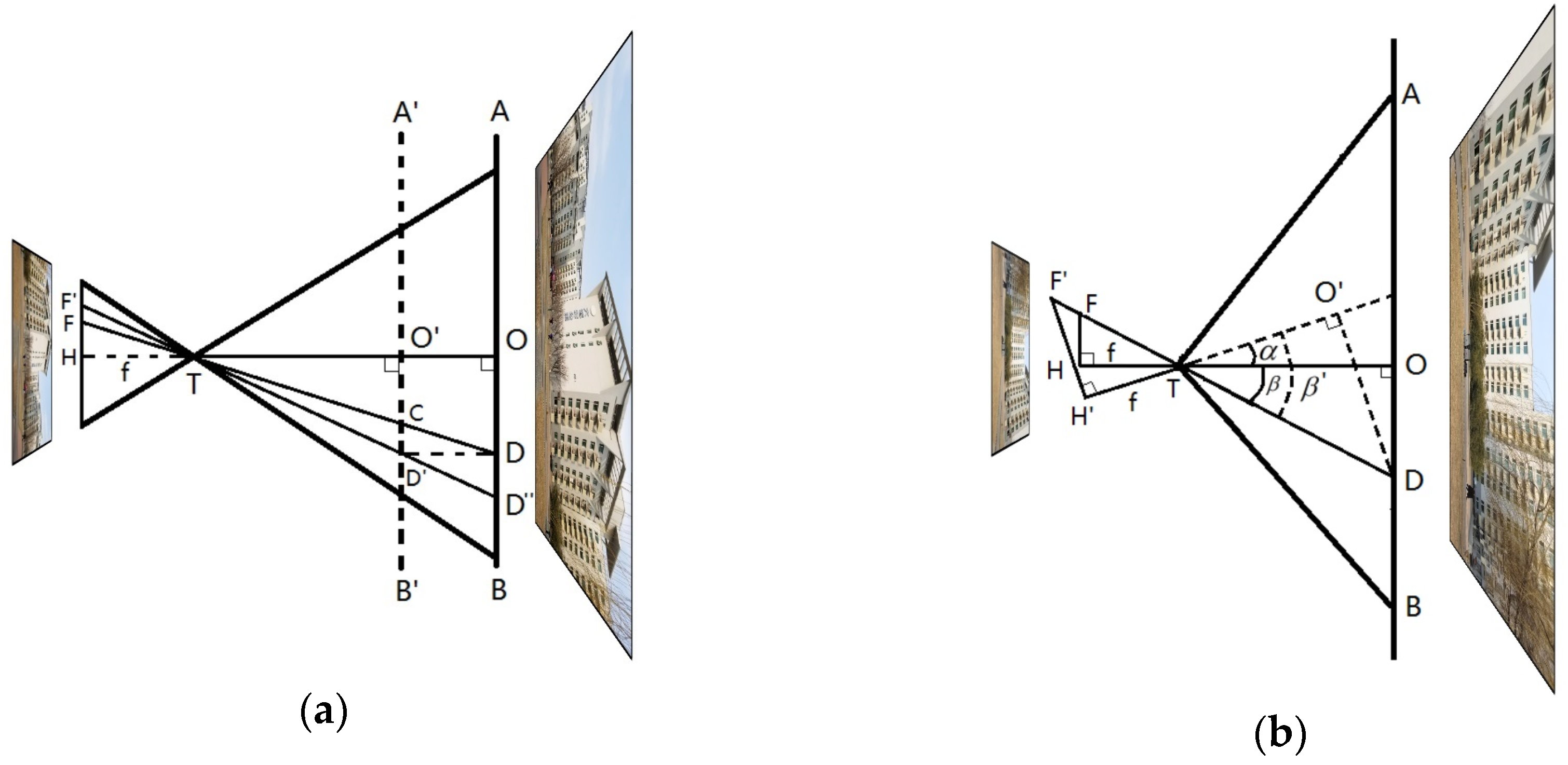
Figure 9.
The iterative structure of the CNN-SIFT hybrid pedestrian navigation. The blocks with a dotted line indicate the global parameter. Each frame will be firstly analyzed by AlphaMEX CNN for the scene classification, then compared with the previous frame to decide whether to run the SIFT-based movement calculation. Routes will be calculated by the global parameter Delay and the walking speed if the scene changed. Movements and routes will be plotted on the map for pedestrian navigation.
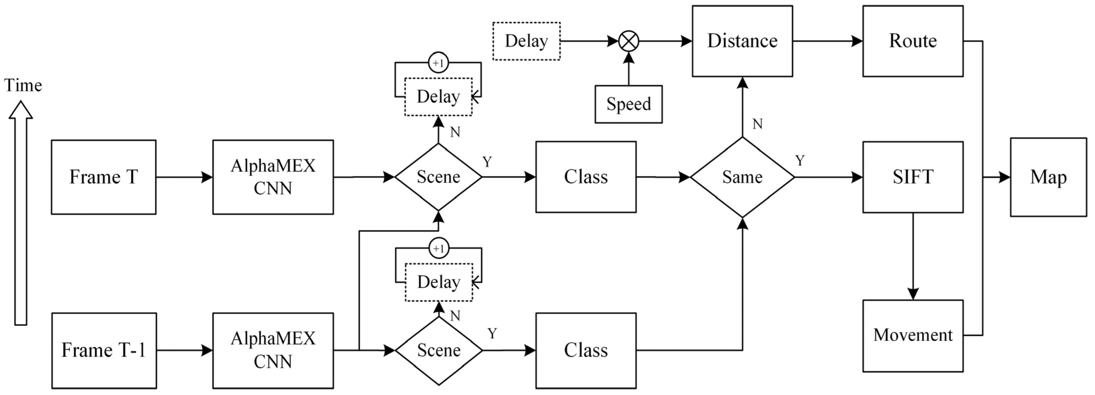
Figure 10.
The AlphaMEX-DenseNet40 architectures for CIFAR. Compared to the original DenseNet40 in Figure 2, the global average pool layer has been replaced by the proposed AlphaMEX Global Pool without changing any other layers.
Figure 10.
The AlphaMEX-DenseNet40 architectures for CIFAR. Compared to the original DenseNet40 in Figure 2, the global average pool layer has been replaced by the proposed AlphaMEX Global Pool without changing any other layers.

Figure 11.
Comparison of the calculated route and the pre-defined route. (a) The pre-defined “Z” shaped route; (b) the calculated route of “Z” shaped test; (c) the pre-defined square route; (d) the calculated route of square shaped test.
Figure 11.
Comparison of the calculated route and the pre-defined route. (a) The pre-defined “Z” shaped route; (b) the calculated route of “Z” shaped test; (c) the pre-defined square route; (d) the calculated route of square shaped test.

Figure 12.
The high resolution BuaaFPV dataset. A total of 13 typical scenes were chosen from BUAA: museum, supermarket, apartment, Heyi building, Dormitory11, gymnasium, high school, clinic, New Main Building, Science Building, concert hall, swimming pool and library. The resolution is 4032 × 3024 in sRGB.

Figure 13.
AlphaMEX CNN-based location estimation result from Apartment to High School. Each dot in the chart represents the confidence of each frame, with different colors representing scene classes (shown in the legend). When the wearer walked in a typical scene area, the algorithm demonstrated the absolute confidence of its estimation (from first frame to 61, 116 to the end), but demonstrated random noise when the wearer walked by the road (62 to 115).

Figure 14.
AlphaMEX CNN-based location estimation result from New Main Building to Concert Hall. Each dot in the chart represents the confidence of each frame with different colors representing scene classes (shown in the legend). The period represents the walking distance, with the wearer walking with constant speed.
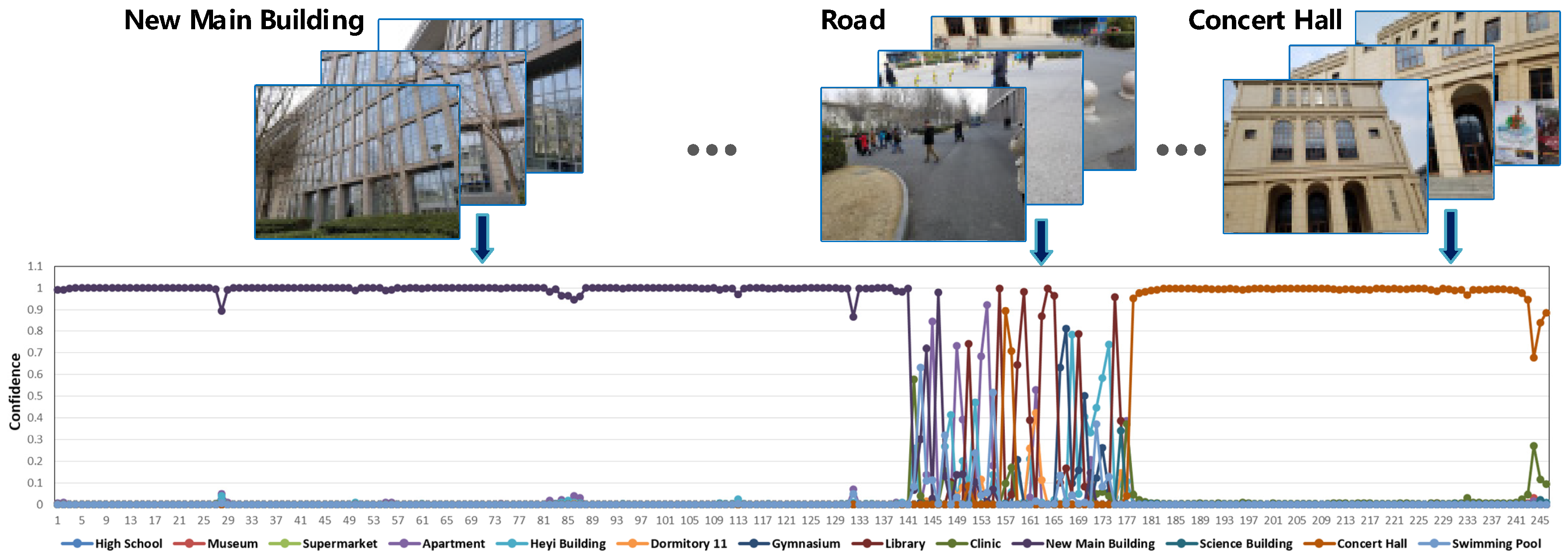
Figure 15.
The FPV clip of “Apartment”. This test clip has several “moving forward” and “rotation” movements, and the whole trajectory resembles a “U” shape. This clip was taken by a wearable camera with 1.5 Hz shooting frequency.
Figure 15.
The FPV clip of “Apartment”. This test clip has several “moving forward” and “rotation” movements, and the whole trajectory resembles a “U” shape. This clip was taken by a wearable camera with 1.5 Hz shooting frequency.
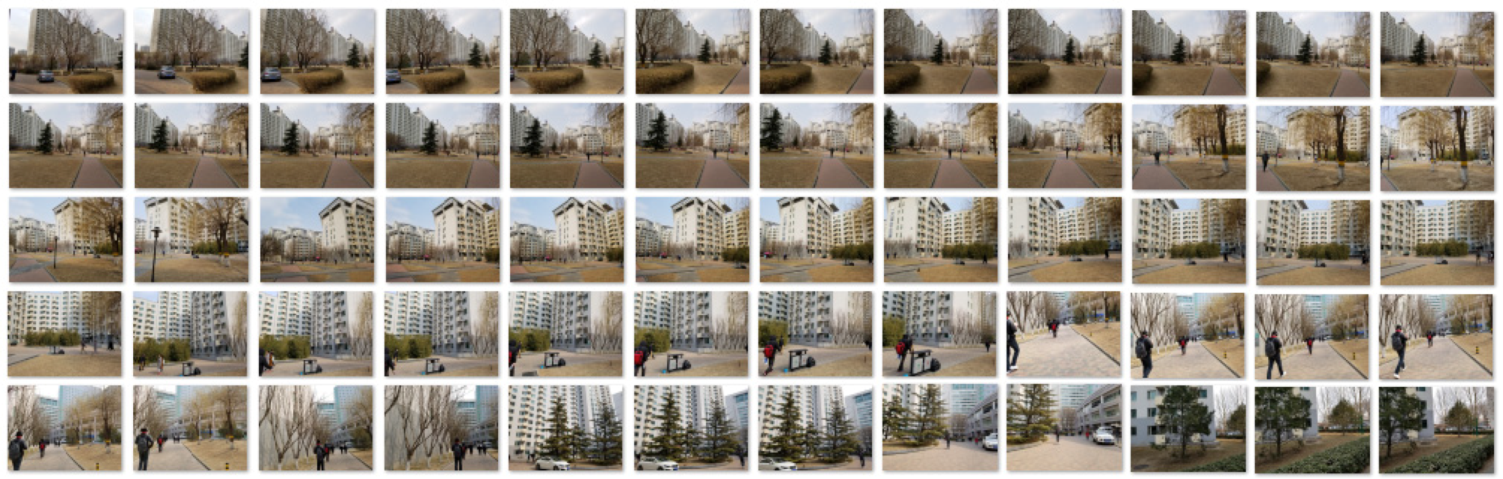
Figure 16.
The FPV based pedestrian navigation result. (a) shows the movement estimation and tracking result; (b) plots the scene recognition result with a route estimation. Orange circles represent the identified scene position and sort by time, while yellow arrows represent estimated routes.
Figure 16.
The FPV based pedestrian navigation result. (a) shows the movement estimation and tracking result; (b) plots the scene recognition result with a route estimation. Orange circles represent the identified scene position and sort by time, while yellow arrows represent estimated routes.
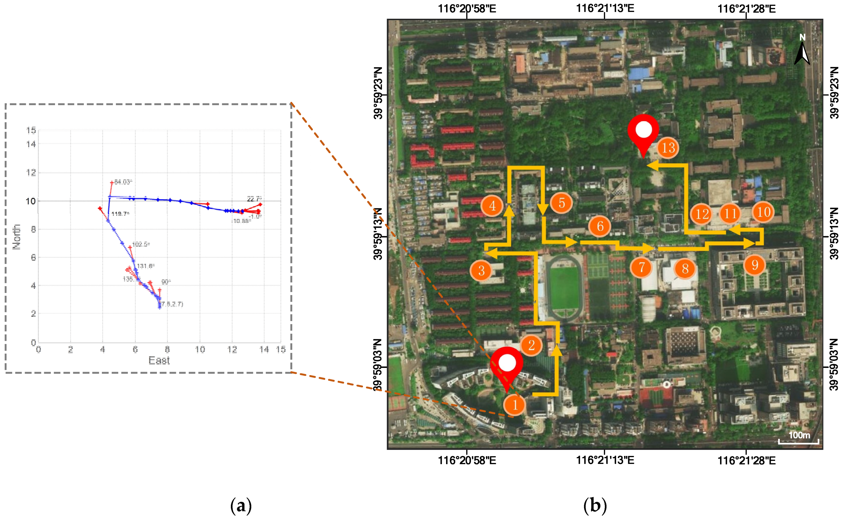
Figure 17.
The FPV-based pedestrian navigation result on the expanded BuaaFPV dataset. (a) plots the scene recognition result with a route estimation; (b) shows the movement estimation and tracking result. Orange circles represent the identified scene position and sort by time, while yellow arrows represent estimated routes.

Table 1.
DenseNet40 and AlphaMEX-DenseNet40 architectures for CIFAR. Error rate is calculated on CIFAR-10 dataset with standard data augmentation.
Table 1.
DenseNet40 and AlphaMEX-DenseNet40 architectures for CIFAR. Error rate is calculated on CIFAR-10 dataset with standard data augmentation.
| Layers | Output Size | Feature-Maps | DenseNet-40 (k = 12) | AlphaMEX-DenseNet-40 (k = 12) |
|---|---|---|---|---|
| Convolution | 24 | conv, stride 1 | ||
| Dense Block (1) | 268 | |||
| Transition Layer (1) | 268 | conv | ||
| 268 | average pool, stride 2 | |||
| Dense Block (2) | 312 | |||
| Transition Layer (2) | 312 | conv | ||
| 312 | average pool, stride 2 | |||
| Dense Block (3) | 456 | |||
| Classification Layer | 456 | global average pool | AlphaMEX global pool | |
| - | - | fully-connected, softmax | ||
| Error rate/F1 score | - | - | 5.24%/95.31% | 5.03%/95.63% |
Table 2.
Error rates (%) on CIFAR-10/CIFAR100 (C10/C100) and SVHN datasets. Standard data augmentation (translation and/or mirroring) is indicated by “+”. The number of model parameters is given in million. AlphaMEX Global Pool-based structures (in bold) achieve lower error rates than each compared state-of-the-art structures without adding redundant layers or parameters.
| Method | Depth | Params (M) | C10 | C10+ | C100 | C100+ | SVHN |
|---|---|---|---|---|---|---|---|
| Network in Network [41] | - | 0.97 | 10.41 | 8.81 | 35.68 | - | 2.35 |
| SimNet [52] | - | - | - | 7.82 | - | - | - |
| Deeply Supervised Net [57] | - | 0.97 | 9.69 | 7.97 | - | 34.57 | 1.92 |
| Highway Network [42] | - | - | - | 7.72 | - | 32.39 | - |
| All-CNN [56] | - | 1.3 | 9.08 | 7.25 | - | 33.71 | - |
| AlphaMEX-All-CNN | - | 1.3 | 8.99 | 7.07 | - | 29.10 | - |
| ResNet [43] | 110 | 1.7 | - | 6.61 | - | - | - |
| ResNet (reported by [58]) | 110 | 1.7 | 13.63 | 6.41 | 44.74 | 27.22 | 2.01 |
| AlphaMEX-ResNet | 110 | 1.7 | 8.41 | 5.84 | 32.87 | 27.71 | 1.97 |
| DenseNet (k = 12) [44] | 40 | 1.0 | 7.00 | 5.24 | 27.55 | 24.42 | 1.79 |
| AlphaMEX-DenseNet (k = 12) | 40 | 1.0 | 6.54 | 5.03 | 27.24 | 23.71 | 1.73 |
Table 3.
Experiments on ImageNet. ResNet architecture is used to compare AlphaMEX Global Pool and global average pool. Top-1 error rate (%) and top-5 error rate (%) are both shown. The difference in error rates is indicated by “Δ”.
Table 3.
Experiments on ImageNet. ResNet architecture is used to compare AlphaMEX Global Pool and global average pool. Top-1 error rate (%) and top-5 error rate (%) are both shown. The difference in error rates is indicated by “Δ”.
| Method | Top-1 | Top-5 |
|---|---|---|
| AlphaMEX Global Pool | 28.1 | 9.1 |
| Global Average Pool | 29.8 | 10.5 |
| Δ | 1.7 | 1.4 |
Table 4.
Calculated Moving Distance and Rotation Angle of “Z” shaped test.
| Moving Forward | Calculated Distance (m) | Actual Distance (m) | Absolute Error (m) | Relative Error (%) |
| part1 | 5.2372 | 5.00 | 0.2372 | 4.74 |
| part3 | 5.5839 | 6.00 | −0.4161 | −6.94 |
| part5 | 2.8602 | 3.00 | −0.1398 | −4.66 |
| Rotation | Calculated Angle (°) | Actual Angle (°) | Absolute Error (°) | Relative Error (%) |
| part2 | 89.2533 | 90.00 | −0.7467 | −0.83 |
| part4 | 92.6742 | 90.00 | 2.6742 | 2.97 |
Table 5.
Calculated Moving Distance and Rotation Angle of square route test.
| Moving Forward | Calculated Distance (m) | Actual Distance (m) | Absolute Error (m) | Relative Error (%) |
| part1 | 18.501 | 19.00 | −0.499 | −2.63 |
| part3 | 28.644 | 30.00 | −1.356 | −4.52 |
| part5 | 12.713 | 13.00 | −0.287 | −2.20 |
| part7 | 20.685 | 20.00 | 0.685 | 3.43 |
| Rotation | Calculated Angle (°) | Actual Angle (°) | Absolute Error (°) | Relative Error (%) |
| 93.2403 | 90.00 | 3.2403 | 3.60 | |
| part4 | 85.8142 | 90.00 | −4.1858 | −4.65 |
| part6 | 87.5610 | 90.00 | −2.4390 | −2.71 |
© 2018 by the authors. Licensee MDPI, Basel, Switzerland. This article is an open access article distributed under the terms and conditions of the Creative Commons Attribution (CC BY) license (http://creativecommons.org/licenses/by/4.0/).
Share and Cite
MDPI and ACS Style
Zhao, Q.; Zhang, B.; Lyu, S.; Zhang, H.; Sun, D.; Li, G.; Feng, W. A CNN-SIFT Hybrid Pedestrian Navigation Method Based on First-Person Vision. Remote Sens. 2018, 10, 1229. https://0-doi-org.brum.beds.ac.uk/10.3390/rs10081229
AMA Style
Zhao Q, Zhang B, Lyu S, Zhang H, Sun D, Li G, Feng W. A CNN-SIFT Hybrid Pedestrian Navigation Method Based on First-Person Vision. Remote Sensing. 2018; 10(8):1229. https://0-doi-org.brum.beds.ac.uk/10.3390/rs10081229
Chicago/Turabian StyleZhao, Qi, Boxue Zhang, Shuchang Lyu, Hong Zhang, Daniel Sun, Guoqiang Li, and Wenquan Feng. 2018. "A CNN-SIFT Hybrid Pedestrian Navigation Method Based on First-Person Vision" Remote Sensing 10, no. 8: 1229. https://0-doi-org.brum.beds.ac.uk/10.3390/rs10081229
Note that from the first issue of 2016, this journal uses article numbers instead of page numbers. See further details here.