Potential Applications of GNSS-R Observations over Agricultural Areas: Results from the GLORI Airborne Campaign

Abstract

The aim of this study is to analyze the sensitivity of airborne Global Navigation Satellite System Reflectometry (GNSS-R) on soil surface and vegetation cover characteristics in agricultural areas. Airborne polarimetric GNSS-R data were acquired in the context of the GLORI’2015 campaign over two study sites in Southwest France in June and July of 2015. Ground measurements of soil surface parameters (moisture content) and vegetation characteristics (leaf area index (LAI), and vegetation height) were recorded for different types of crops (corn, sunflower, wheat, soybean, vegetable) simultaneously with the airborne GNSS-R measurements. Three GNSS-R observables (apparent reflectivity, the reflected signal-to-noise-ratio (SNR), and the polarimetric ratio (PR)) were found to be well correlated with soil moisture and a major vegetation characteristic (LAI). A tau-omega model was used to explain the dependence of the GNSS-R reflectivity on both the soil moisture and vegetation parameters.

1. Introduction

In agricultural areas, soil surface and vegetation cover conditions play an essential role in the understanding of processes related to the soil-vegetation-atmosphere interface, and in different applications related to agricultural management [1,2,3,4]. Although optical remote sensing is highly sensitive to features such as the vegetation cover characteristics, it is strongly affected by the diurnal cycle and weather conditions (cloud cover, etc.) [5]. Active and passive microwave remote-sensing techniques are thus an important source of data, for which numerous studies have proposed various inversion algorithms for soil and vegetation characterization, including operational estimations [6,7,8,9,10,11,12]. The Global Navigation Satellite System-Reflectometry (GNSS-R) is a microwave technique based on bistatic radar observations, which appeared at the beginning of the 1990s. GNSS-R makes opportunistic use of the signals emitted by global satellite navigation constellations, such as the Global Positioning System (GPS) [13]. Although this technique was initially used for oceanographic applications, various experimental in situ and airborne campaigns have led to a considerably improved understanding of the interaction of these signals with the Earth’s surface, and their potential for monitoring land surface conditions, including that of the cryosphere [14]. In recent years, the GNSS-R technique has been increasingly tested and validated over land surfaces [15,16,17,18,19,20,21], using either single antenna reflected signal-to-noise-ratio (SNR) measurements from commercial geodetic instruments, or dedicated multi-antenna configurations combined with the analysis of correlation waveforms and/or delay-Doppler maps (DDMs).

Focusing on the estimation of soil moisture and vegetation parameters, different studies have been conducted over the last ten years [16,17,18,19,20,21,22,23,24]. Observations and analyses conducted during the SMEX02 campaign were, to the best of our knowledge, the first large-scale attempt to investigate the airborne potential of GNSS-R for the remote sensing of soil moisture. Using a single-polarization, left-hand circular polarization (LHCP) antenna for nadir-pointing observations, the aircraft flew at approximately 1100 m above ground level (AGL) with a velocity of ~75 m/s over an area where the ground and vegetation parameters were monitored. The authors have computed the GNSS-R signal’s sensitivity to lie between 10 and 30 dB per m³/m³ of surface soil moisture. They also observed and modeled the attenuation produced by the vegetation cover, but they did not perform an in-depth investigation of the system’s sensitivity to this parameter. In 2009, the LeiMON campaign [16] was performed over a period of more than six months in order to assess the sensitivity of polarimetric GNSS-R observations to soil roughness, soil moisture and vegetation, using a ground-based instrument attached to a mast 25 m above the ground. During the course of the experiment, the soil moisture and roughness conditions varied over a wide range, and the only monitored crop was sunflower. The sensitivity of the cross-polarization (right-left) reflectivity $({\Gamma }_{RL})$ to soil moisture content was confirmed to be 20 to 30 dB/(m³/m³) for low to moderate surface roughness conditions, with a root mean square surface height (Hrms) below 3 cm, and its sensitivity to vegetation water content (VWC) was estimated to be ~0.3 dB/(kg/m²). The use of observations based on the ratio of ${\Gamma }_{RR}$ (co-polarization reflection coefficient) to ${\Gamma }_{RL}$ to retrieve soil moisture was shown to limit the effect of roughness conditions. However, as pointed out by the authors, instrumental improvements to avoid saturation at reflectivities below −17 dB were needed to confirm their results.

In an effort to validate these results over a larger area, including various crops and several forest sites, the instrument described in [16] was upgraded and installed on an aircraft for the GRASS campaign organized in Italy [25,26], during which GNSS-R measurements were recorded from an aircraft at 150 m AGL. These observations confirmed the strong potential of GNSS-R techniques for the estimation of not only soil moisture, but also forest biomass. The instrument’s sensitivity to soil moisture was confirmed to be on the order of 20 dB/(m³/m³), with a determination coefficient between the ground moisture measurements and the GNSS-R reflectivity polarization ratio equal to 0.86. In the case of forest biomass estimations, the observed sensitivity was approximately 0.015 dB/(Mg·ha⁻¹), with a correlation coefficient (R²) of 0.91 between the ground measurements and the cross-polarization reflection coefficient $({\Gamma }_{RL})$. The system’s sensitivity to VWC could not be accurately determined, due to a lack of ground-truth data. Sanchez et al. [18] have confirmed the potential of GNSS-R reflectivity to retrieve soil moisture, using LARGO airborne measurements over an agricultural area in Spain. A multiple regression model was proposed to link soil moisture to the surface temperature, the vegetation index and the LARGO reflectivity. This study is based on one day measurements with soil moisture limited to low values below 0.15 m³/m³.

In the last two years, the use of GNSS-R has gained new momentum with the launch of several spaceborne missions with GNSS-R capabilities, such as TechDemosat in 2014, SMAP in 2015 and CYGNSS in 2016, and various studies have already demonstrated the considerable potential of these instruments for the estimation of land surface parameters [19,27,28,29]. Camps et al. [19] demonstrated the sensitivity of TechDemosat data to soil moisture and vegetation. For nearly bare soils, they retrieved a high sensitivity of GNSS-R scattered power to soil moisture (~38 dB/(m³/m³)). The sensitivity of TechDemosat data to soil moisture has been confirmed by Chew et al. [28] with a 7 dB dynamic due to changes in soil moisture.

The GLORI’2015 campaign [30] analyzing agricultural land in the present paper was designed to confirm the results obtained during the aforementioned studies, to generate a dataset allowing some of the limitations encountered in these studies to be avoided and to deepen the understanding of the GNSS-R physical signal, an essential step to propose operational satellite algorithms for land surface properties mapping.

Accurate polarimetric GNSS reflected signals were measured over agricultural plots and were accompanied by high temporal and spatial resolution of in situ sampling of the soil and vegetation parameters. In the present analysis, the potential use of three different GNSS-R observables (apparent reflectivity $({\Gamma }_{RL})$, reflected signal (SNR), and the reflectivity polarization ratio) for the monitoring of the soil and vegetation is discussed, which was not possible in the context of previous campaigns. A large ground-truth database, including data corresponding to a wide range of soil moisture values and various types of vegetation cover, was collected during the GLORI’2015 campaign to confirm several important results retrieved from smaller databases, such as those reported in [30].

In the second section, we present the study site, the airborne and ground measurements and the GNSS-R data processing. In Section 3, we analyze the correlations observed between in situ data and GNSS-R measurements. Section 4 discusses results obtained for modeling and inversion of GNSS-R reflectivity. Our conclusions are presented in Section 5.

2. Dataset and Methods

2.1. GNSS-R Airborne Data

2.1.1. Instrument

The airborne GNSS-R data presented in this study were recorded with the GLORI instrument during the GLORI’2015 Campaign [30]. The GNSS-R GLORI instrument, developed by the CESBIO, is a polarimetric device with four channels. Two antennas are connected to the receiver: the first of these is pointed towards the zenith, to receive the direct RHCP (right-hand circular polarization) signals transmitted by GNSS satellites; the second ‘nadir’ antenna is pointed vertically downwards, to receive the signals reflected from the ground in two polarizations (RHCP and left-hand circular polarization (LHCP)). A transfer switch is used to perform the relative calibration of these polarimetric measurements. The nadir antenna is qualified in terms of its cross-polarization isolation between the LHCP and RHCP signals. The cross-polarization isolation is better than 15 dB up to 45° from boresight (45° elevation) for both LHCP and RHCP ports. Below 15 dB of cross-polarization, the performance is considered insufficient to perform polarimetric measurements [30].

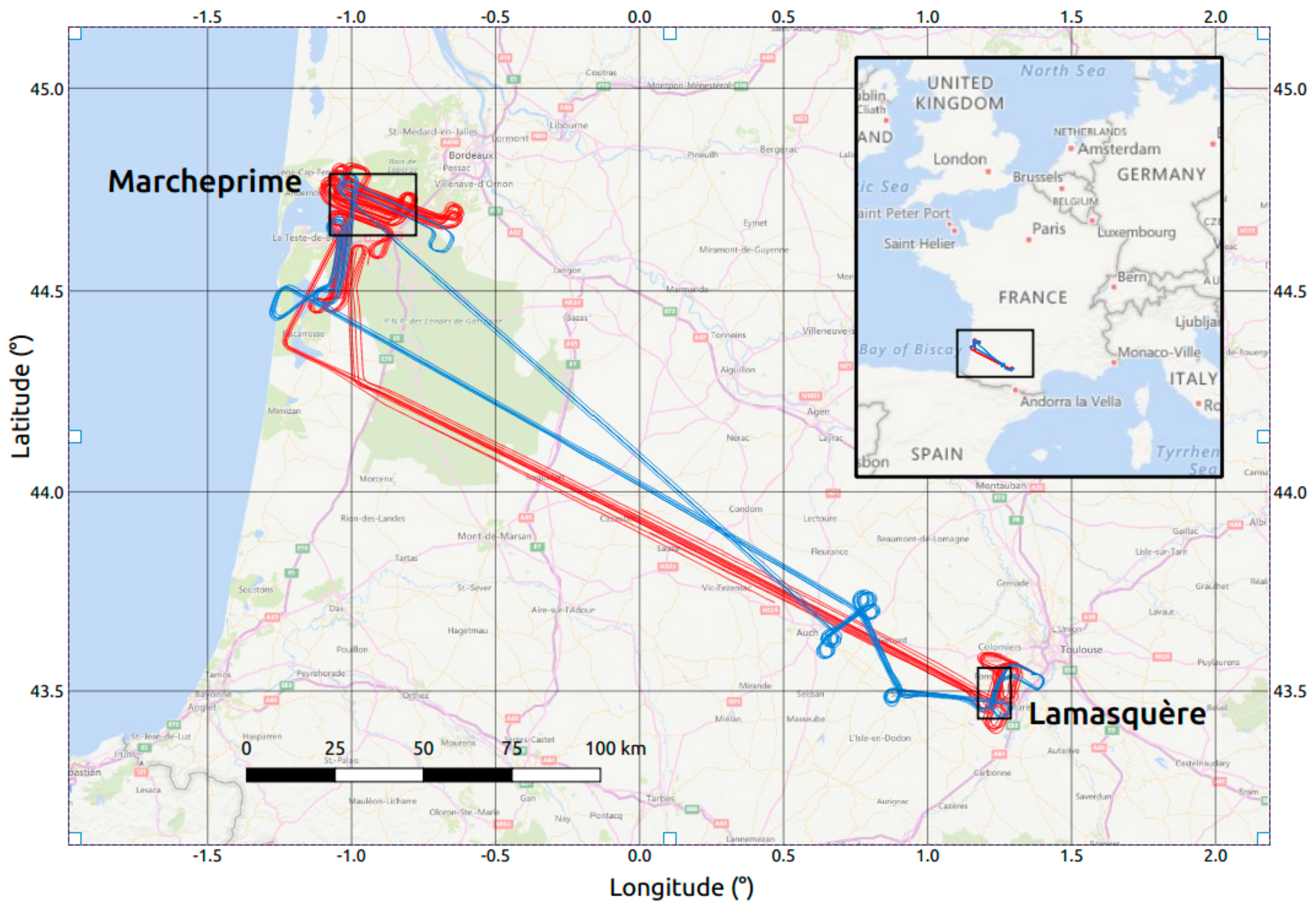
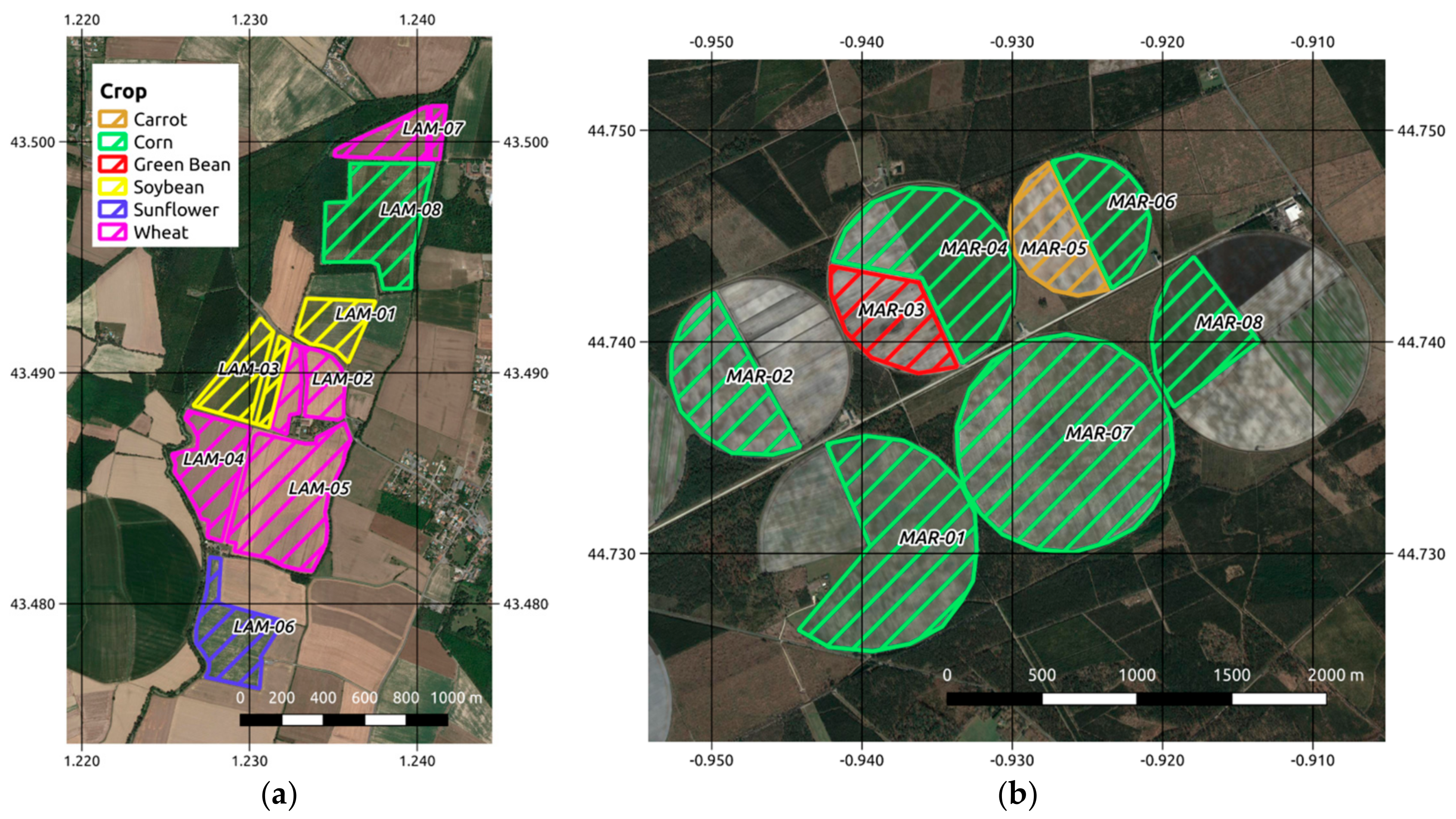
2.1.2. Airborne Campaigns

Five scientific flights were made above the studied site (Figure 1), over a period of two weeks (22 June–6 July 2015). The aircraft flew at a speed of ~100 m/s, and an altitude of ~600 m above the ground. The antenna radiation patterns allowed measurements to be made at all elevations between 30° and 90°. Three synchronized streams of raw data, centered on the GPS L1 frequency (1.57 GHz), were continuously acquired at 10 MSPS: one from the zenith-pointing RHCP antenna and two from the nadir-pointing antenna, in the RHCP and LHCP polarizations. The data were then processed offline to extract the GPS L1 signal waveforms, with a coherent integration time of 20 ms. After correcting for the antenna radiation pattern and receiver noise [30,31], the individual waveform maxima were averaged incoherently for 240 ms, allowing the GNSS-R observables to be computed.

The study sites were located in the southwest of France (Figure 1). This region is characterized by a temperate climate, with annual rainfall ranging from 600 mm to 900 mm and a mean maximum daily air temperature close to 19 °C in summer. Two agricultural sites, Lamasquère and Marcheprime, were considered. The reference fields were sampled among various crops (wheat, sunflower, corn, soybean, carrots, green bean) presenting a wide range of cover characteristics during the two weeks of the airborne campaign.

• The Lamasquère site (43.49°N, 1.23°E, Figure 2a) included eight fields (four wheat, two soybean, one corn and one sunflower)
• The Marcheprime site (44.74°N, 0.93°W, Figure 2b) included nine fields (seven corn, one green bean and one carrot).

2.2. In Situ Data

Intensive, collocated ground-truth measurements were recorded at the same time as the flights were made over the two agricultural sites of interest. The in situ measurements made at the reference fields were designed to determine the soil moisture and vegetation characteristics (leaf area index, vegetation height).

2.2.1. Soil Moisture

Soil moisture measurements were carried out simultaneously with the airborne acquisitions. For each reference field, approximately twenty measurements were made for each airborne acquisition. These were recorded using a handheld Thetaprobe, at depths between 0 and 5 cm. Due to the high evaporation rates present in this area, the soil moisture measurements were made within a time window of two hours prior to or following the airborne measurements. The soil moisture was then computed as the mean value of all soil measurements recorded for the same field. The soil moisture ranged between 0.04 and 0.27 m³/m³ during the ground campaigns (

Table 1. Range of variation in soil moisture, leaf area index (LAI) and vegetation height (VH) during GLORI campaigns.

Date (dd/mm/yy)	Soil Moisture (m3/m3)	LAI (m²/m²)	VH (cm)
22/06/2015	[0.04–0.23]	[0–5.5]	[0–104]
25/06/2015	[0.1–0.22]	-	-
29/06/2015	[0.04–0.24]	[0–6.5]	[0–203]
01/07/2015	[0.08–0.21]	[0–6.18]	-
06/07/2015	[0.09–0.23]	[0–6.8]	[0–257]

). It should be noted that there was no precipitation during the 15 days of the campaign.

2.2.2. Vegetation

To characterize the vegetation cover for all reference fields, two types of measurements were performed during the airborne acquisitions: the leaf area index (LAI), and the vegetation height (VH).

• Leaf area index

The leaf area index (LAI) is defined as the total one-sided area of green leaves per unit horizontal ground area. The LAI was estimated from the analysis of the directional canopy gap fraction measured from hemispherical digital photography. For each field, 12–25 hemispheric digital photographs were acquired at the same time as the flights. Mean LAI values observed for all reference fields ranged between 0 and 6.8 during the GLORI campaigns (Table 1). The value of zero corresponds to the wheat crops, which were senescent.

• Vegetation height

The canopy height was measured over twenty or thirty plants for each reference field, twice at the Lamasquère site, and three times at the Marcheprime site. The mean value of the height was considered for each field, and it ranged between 0 and 257 cm during the GLORI campaigns (Table 1). The value of zero corresponded to the wheat fields.

2.3. GNSS-R Data Processing

The GLORI processing chain comprises eight main steps and makes use of the raw data stream, and the GPS ephemeris and flight ancillary data as inputs [30,31]:

• GNSS processing of the raw data stream
• Acquisition and tracking of the modulated signal to compute correlation waveforms
• Time tagging and extraction of waveform maxima as described in [32]
• Processing of the navigation message to recover the transmission time, and extraction of the correlation power
• Instrument corrections and incoherent averaging
• Correction for antenna gain and instrumental noise, incoherent averaging and reflectivity computation
• Geo-location and merging of individual files
• Computation of the location and surface shape of each footprint, merging of individual measurements into a consolidated file

Three observables were considered in our analysis of the GNSS-R sensitivity to the land surface parameters: the apparent reflectivity, the processing signal-to-noise-ratio (SNR) of the reflected signal and the polarimetric ratio.

The apparent reflectivity is related to the fraction of power reflected by the ground [16]. For a polarization pq (p and q denote the incident and the scattered, respectively), the apparent reflectivity ${\Gamma }_{pq}$ can be expressed as the ratio of the reflected $Y_{ref,q}$ to the direct waveform $Y_{dir,p}$. In the case of GNSS-R, the right-right (RR) and right-left (RL) ratios represent the co- and cross-polarization reflection coefficients, ${\Gamma }_{RR}$ and ${\Gamma }_{RL}$:

$${\Gamma }_{pq}=\frac{{|\langle Y_{ref,q}\rangle |}^2}{{|\langle Y_{dir,p}\rangle |}^2}$$

(1)

The processing signal-to-noise-ratio (SNR) of the reflected signal defined as the signal power (above the noise floor), divided by the noise level:

$$SNR=\left(\left|Y_{r,max}\right|-B_r\right)/B_r$$

(2)

where $B_r$ is the waveform noise floor and $Y_{r,max}$ is the maximum of the reflected waveform.

The polarimetric ratio (PR) is defined as the ratio of both apparent reflectivities ${\Gamma }_{RR}$ and ${\Gamma }_{RL}$:

$$PR={\Gamma }_{RL}/{\Gamma }_{RR}$$

(3)

The scattered signal consists of two components, the coherent and incoherent terms. The first of these is related to the Fresnel zone, whereas the second covers an area much larger than the Fresnel zone, the so-called glistening zone. The latter component is reduced in the calculation of apparent reflectivity. The values of apparent reflectivity ${\Gamma }_{pq}$ are thus associated with the Fresnel zone, which is elliptical and has a semi-major axis defined by:

$$ra=\sqrt{\lambda h\sin \theta }/{\sin }^2 \theta$$

(4)

where λ is the signal’s wavelength, h is the aircraft’s height above the ground, and θ is the elevation angle.

In the present case, the aircraft flew at an altitude of 600 m, such that for an elevation angle equal to 60°, ra was approximately 13 m for the L1 signal. These dimensions show that it should be possible to analyze the behavior of GNSS-R signals scattered by reference fields a few hectares in size. For the purpose of spatial co-location, all of the 240 ms incoherently averaged GNSS-R measurements were mapped onto ellipses, defined according to the size of their first Fresnel zone, and elongated in the flight direction. These footprints were then tested for their enclosure within imaginary polygons (allowing for an additional 20 m buffer, i.e., ~1.5 ra) delimiting the plots. In the present study, to avoid the potential influence of strong noise resulting from cross-polarization isolation degradation for elevation angles lower than 50° [30], as well as multi-scattering effects with the direct and reflected signals (as described in [32]), elevations ranging between 50° and 90° only were considered.

3. Data Analysis

Several theoretical studies have shown that the elevation angle has an influence on the bistatic signal penetration down to the soil and the retrieval of vegetation parameters [33,34]. For this reason, our statistical analysis of the GNSS-R measurements makes use of two elevation intervals (50–70° and 70–90°). Although this dependence on elevation could be reduced through the selection of a narrower range of values, 20° intervals were used in the present study to maintain a sufficiently high number of samples in each interval.

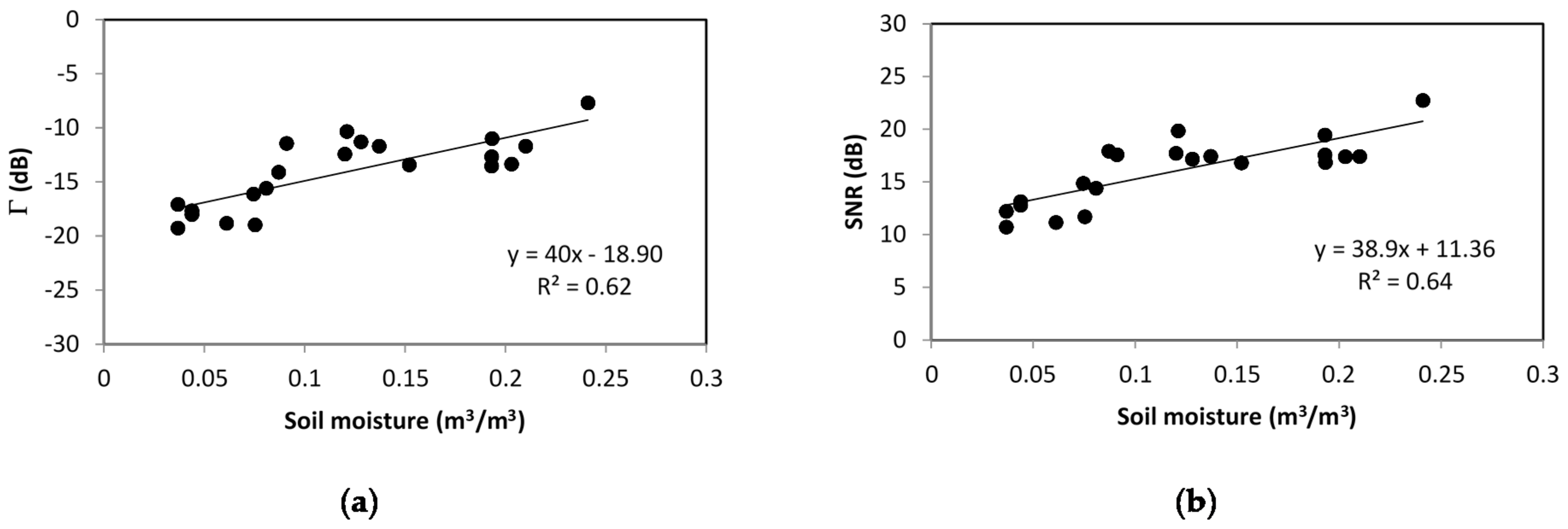
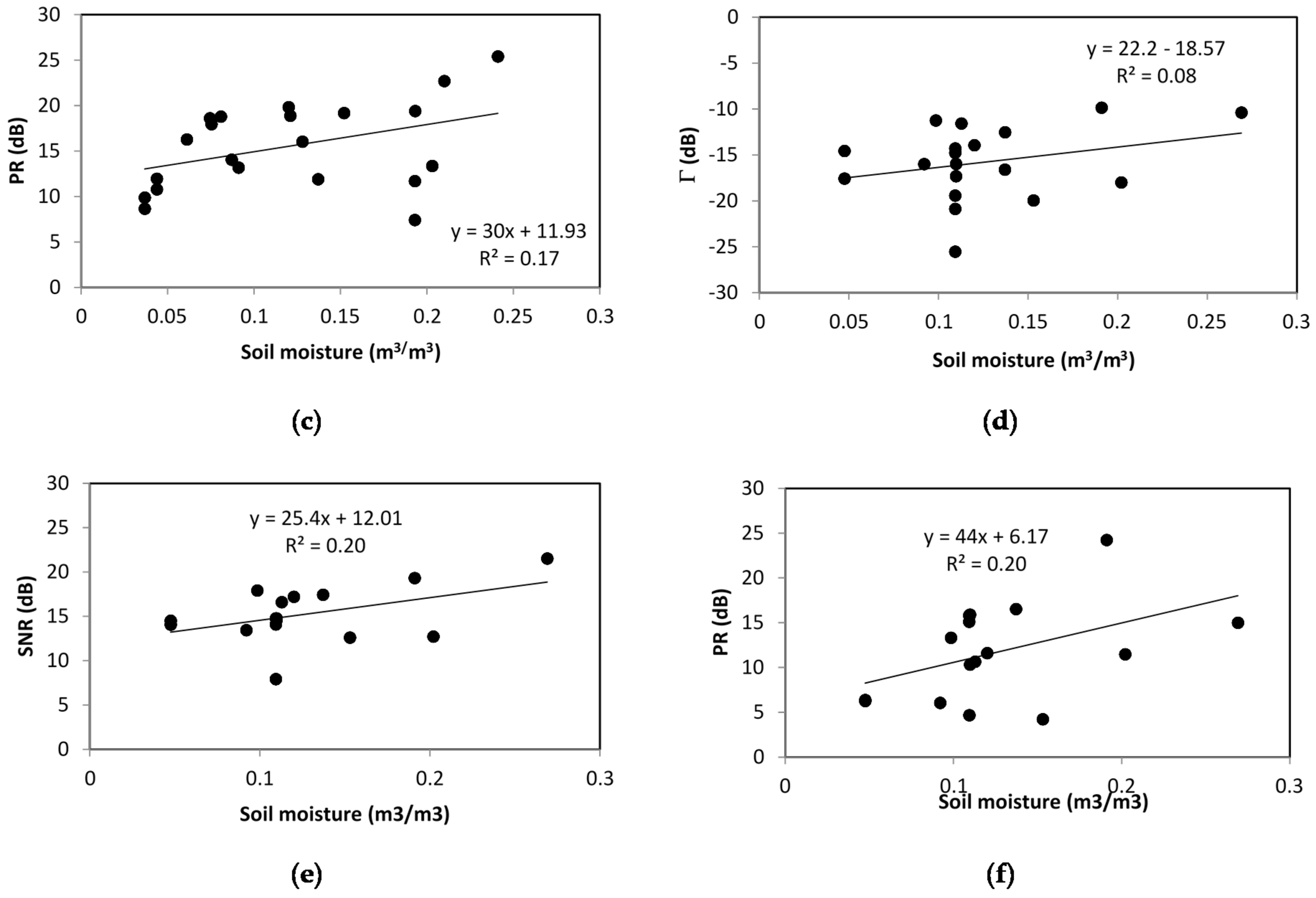
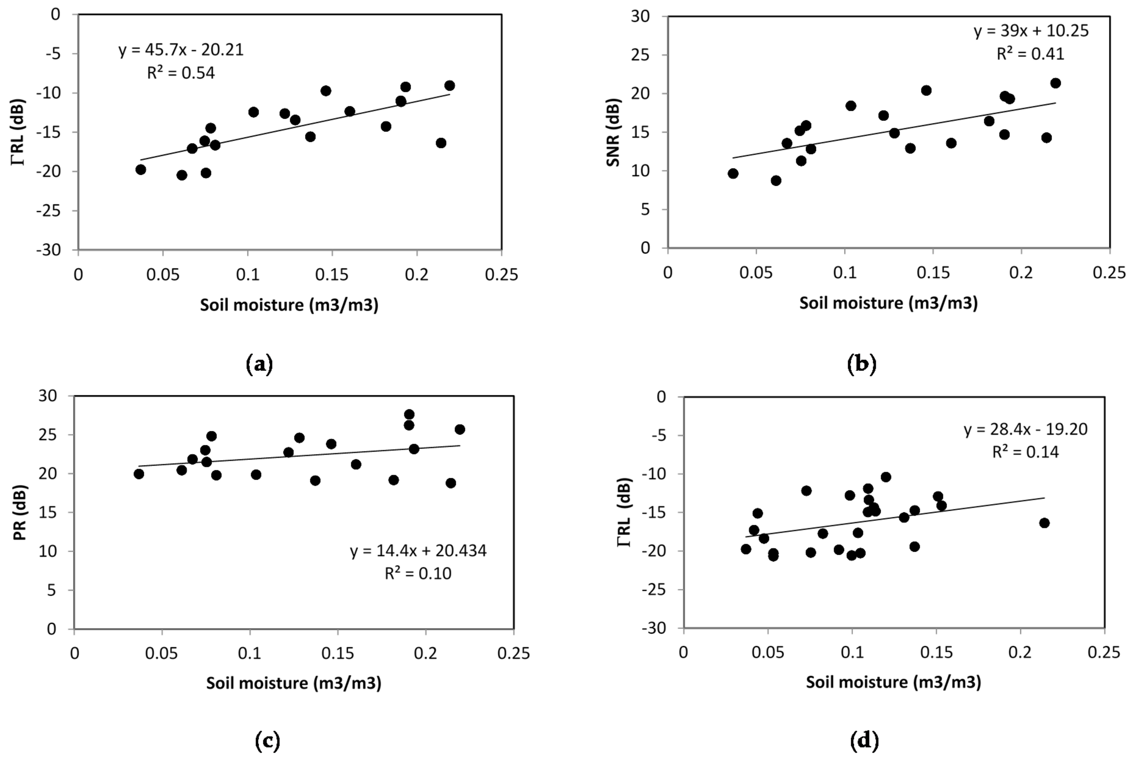
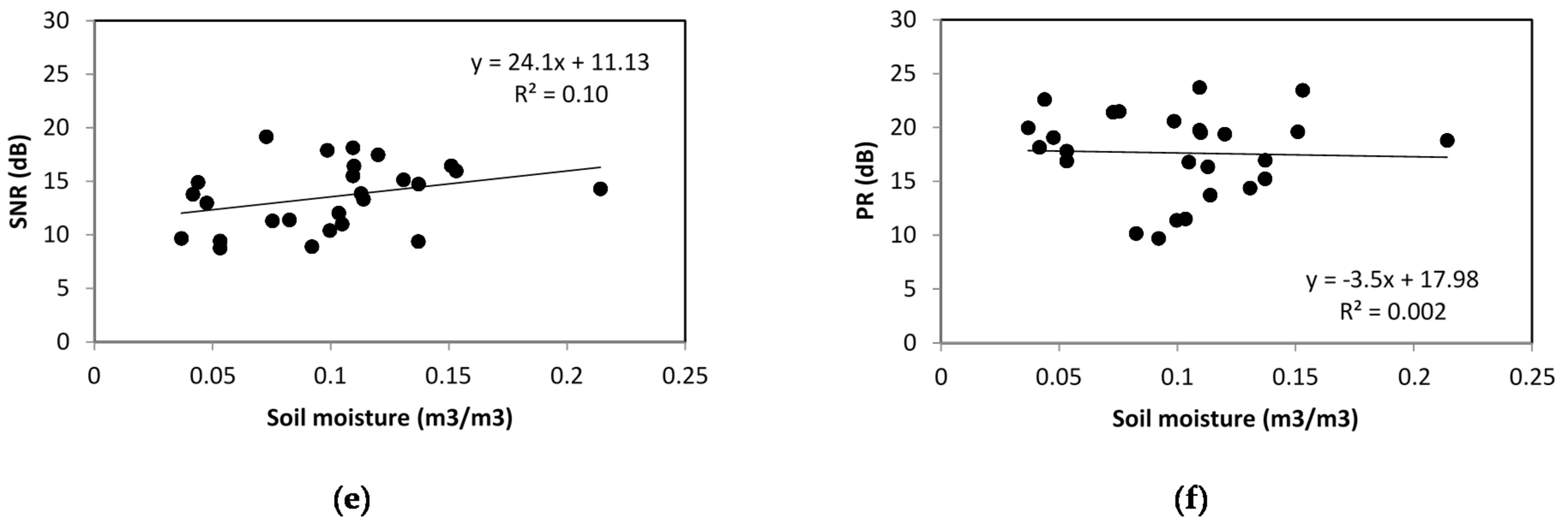
3.1. Relationships between GNSS-R Observables and Soil Moisture

To minimize the influence of heterogeneity in the vegetation characteristics between the reference fields, the sensitivity of the GNSS-R observables to soil moisture were analyzed for two classes of LAI. The first of these was defined by LAI < 1, corresponding to sets of 22 and 19 GNSS-R measurements over the reference fields with bare or poorly vegetation-covered soils for the two elevation angle intervals (50–70°) and (70–90°). The second class is defined for LAI > 1, corresponding to sets of 14 and 25 GNSS-R measurements over the reference fields with medium and high vegetation densities for the two elevation angle intervals (50–70°) and (70–90°), respectively.

Figure 3 and Figure 4 show ${\Gamma }_{RL}$, the reflected SNR and PR as a function of soil moisture, for the two LAI classes. Each plotted point represents a GNSS-R mean measurement on a reference field at a given date. The number of samples is different from that of the reference fields; it varies from one measurement configuration to another. The sensitivity of GNSS-R observables to soil moisture can be seen to generally decrease with increasing LAI. The vegetation component, which attenuates the signal scattered by the soil, thus influenced the GNSS-R signal sensitivity to variations in soil moisture. As an example, for the 70–90° elevation interval, the ${\Gamma }_{RL}$ sensitivity to soil moisture (S) decreased from 45.7 dB/(m³/m³) for the weak LAI values (LAI < 1) to 28.4 dB/(m³/m³) for the highest LAI values (LAI > 1). The same behavior was observed for reflected signal SNR, with the decreasing of sensitivity from 39 to 24.1 dB/(m³/m³), from weak LAI values to high LAI values, for the same elevation angle interval (70–90°). The dynamic range of the GNSS-R signals was greater than 10 dB for reflectivity and SNR. For the case of ${\Gamma }_{RL}$ and reflected signal SNR, the retrieved sensitivity was greater than that in the case of the Leimon and GRASS campaigns, which reported values of ~20 dB/(m³/m³) [25,26]. They were in agreement with values retrieved in [19] using TechDemosat data (38 dB/(m³/m³)).

With the decrease of S with increasing LAI (i.e., vegetation cover development), we also observed a decrease in the correlation coefficient between GNSS-R observables (${\Gamma }_{RL}$ or reflected SNR) and soil moisture. For example, the correlation between ${\Gamma }_{RL}$ and the moisture decreased for the 70–90° elevation angle range from R² = 0.54 for LAI < 1 data to R² = 0.14 for LAI > 1 data. This result clearly illustrates the effect of noise generated by the vegetation contributing to the GNSS-R observables. This relatively low correlation value could also be attributed to differences in the scattering behavior between the various types of vegetation cover observed during the campaign (i.e., different crop species, cultivars, or development stages).

For the case of PR, we observed a low correlation with soil moisture (R² < 0.2, even for low LAI values). This correlation suggests that, in airborne scenarios, the polarimetric ratio has a lower sensitivity to soil moisture, contrary to the findings reported for the example in [26]. This difference could be explained by the fact that the GLORI measurements were corrected for cross-polarization effects, thus removing most of the residual LHCP signal contributions from the RHCP reflected antenna. This limitation could be due to the high noise level in the PR data, coming from low values of ${\Gamma }_{RR}$. For this reason, it seems difficult to consider this observable in the analysis of soil moisture effect.

Concerning the dependence on the elevation angle for the two observables (reflectivity and SNR) we observed a sensitivity slightly higher for high elevation angles in the case of a low LAI class with sensitivity of reflectivity to soil moisture; for example, equal to 45.7 dB/(m³/m³) for 70–90° and 40 dB/(m³/m³) for 50–70°, and approximately the same for SNR (equal to 39 dB/(m³/m³) for 70–90° and to 38.9 dB/(m³/m³) for 50–70°). This sensitivity is attributed to the vegetation’s influence and its high attenuation of GNSS-R signals at lower elevation angles.

Table 2. Statistical parameters of relationships between GNSS-R observables and soil moisture, for two vegetation class conditions (LAI < 1 and LAI > 1), and two elevation angle intervals (50–70° and 70–90°). S = the sensitivity of GNSS-R observables to soil moisture. R² = correlation coefficient.

	50–70°				70–90°
	LAI < 1		LAI > 1		LAI < 1		LAI > 1
	S dB/(m3/m3)	R2	S dB/(m3/m3)	R2	S dB/(m3/m3)	R2	S dB/(m3/m3)	R2
${\Gamma }_{RL}$	40	0.62	22.2	0.08	45.7	0.54	28.4	0.14
SNR	38.9	0.64	25.4	0.20	39	0.41	24.1	0.10
PR	30	0.17	44	0.20	14.4	0.10	−3.5	0.01

summarizes all the results of the GNSS-R observable sensitivities to soil moisture for the different configurations discussed above.

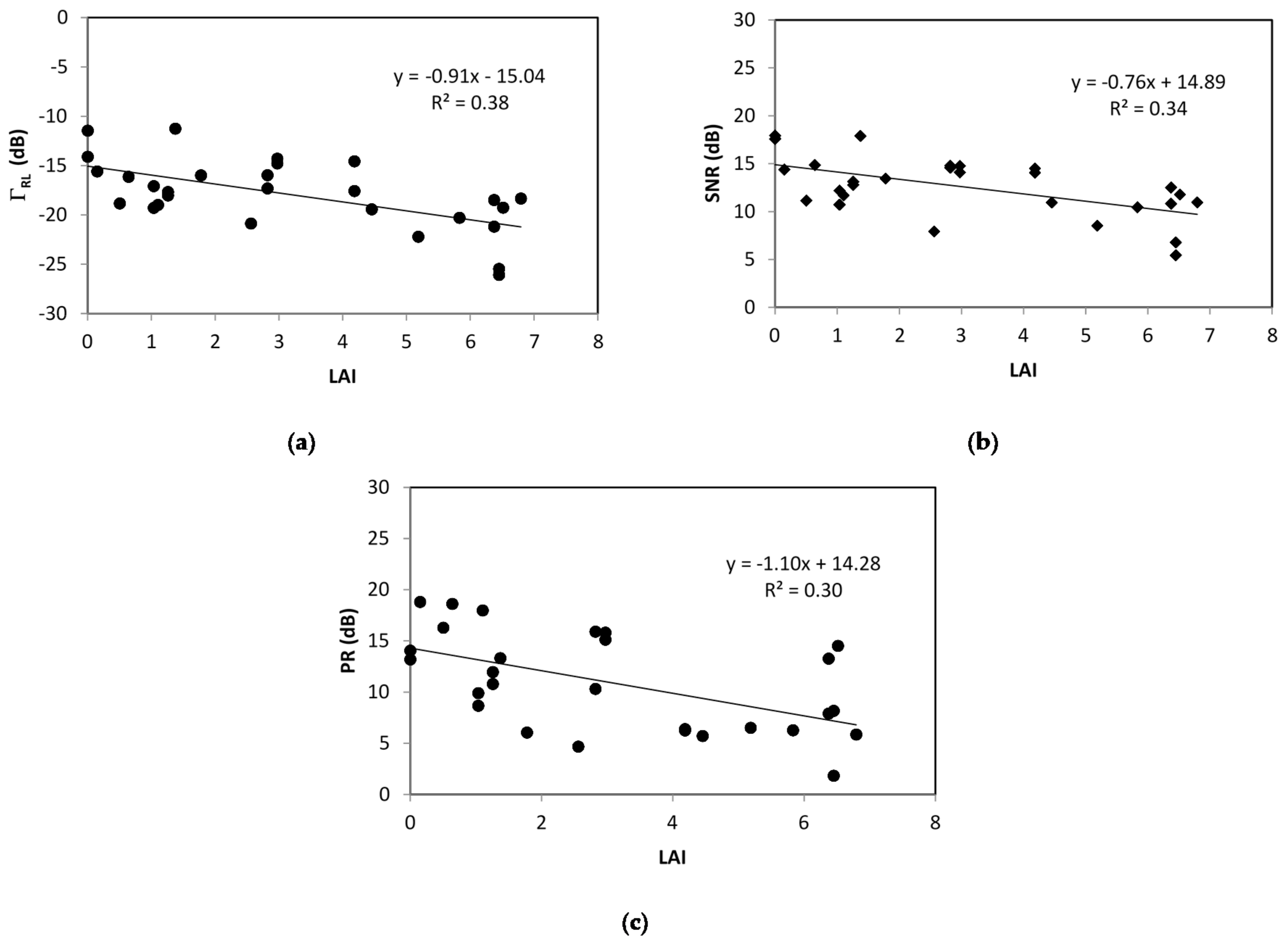
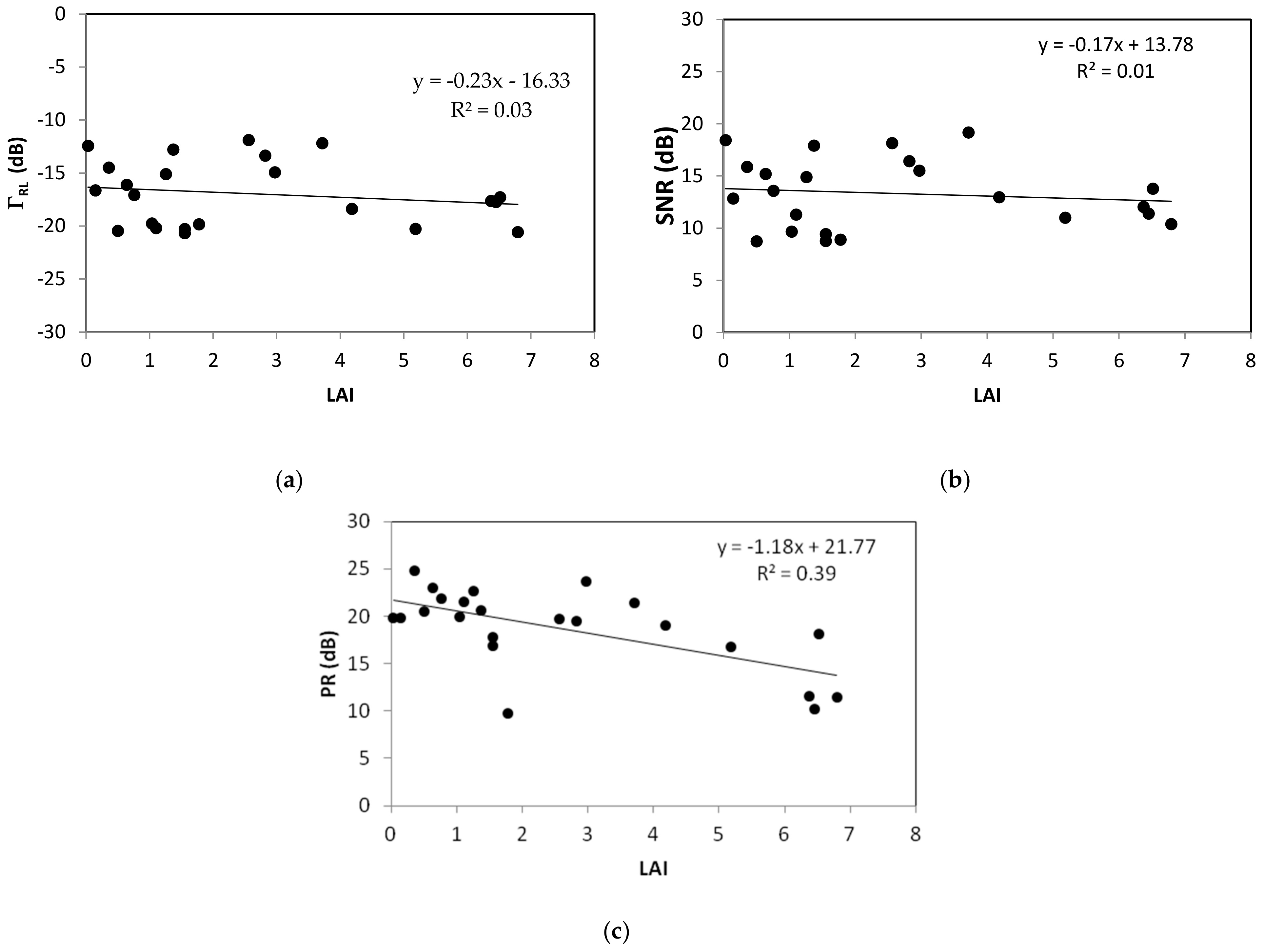
3.2. Relationships between GNSS-R Observables and Vegetation Parameters

In this section, the GNSS-R observables are analyzed as a function of one specific vegetation parameter, namely, the LAI of the plant cover. As in the case of soil moisture, two elevation angle intervals (50–70° cf. Figure 5 and 70–90° cf. Figure 6) and three observables (${\Gamma }_{RL}$, LHCP SNR, and polarimetric ratio) were considered. To avoid effects due to soil moisture, we considered data corresponding to dry conditions, with soil moisture lower than 0.1 m³/m³. In the database used for the present study, since a small number of bare soil measurements were found to correspond to the wet moisture values (Mv), an additional second class, with Mv > 0.2 m³/m³ was not considered.

Figure 5a and Figure 6a show the sensitivity of ${\Gamma }_{RL}$ to the vegetation LAI for the reference fields with dry soil conditions (sets of 28 and 23 samples for the two elevation angle intervals (50–70° and 70–90°), respectively). Each sample represents a GNSS-R mean measurement on a reference field at a given date. There is a clear decrease in this GNSS-R observable intensity with increasing vegetation LAI, due to the influence of signal scattering and attenuation (increasing optical thickness). Dynamic ranges between 5 and 10 dB are observed for the 50–70° and 70–90° elevation angles, respectively. The observed higher sensitivity (Sv) at low elevation angles (Sv equal to −0.91 dB/(m²/m²)) can probably be attributed to a decrease in the influence of the soil component (roughness and moisture) due to an increase in the vegetation optical depth. This sensitivity is accompanied by an increase in the correlation between GNSS-R signals and vegetation LAI, with R² equal to 0.38 at low elevations, and only 0.03 at high elevations for the case of reflectivity. A similar behavior is observed for the reflected signal SNR, as shown in Figure 5b and Figure 6b, which reveals a dynamic range of approximately 5–10 dB, a sensitivity equal to −0.76 dB/(m²/m²) for the elevation angles 50–70° range and reduced to −0.17 dB/(m²/m²) for the elevation angles of 70–90°.

The PR observable is found to be correlated with the vegetation LAI (Figure 5c and Figure 6c), with a high sensitivity to vegetation LAI equal to −1.1 dB/(m²/m²) for low elevation angles and to −1.18 dB/(m²/m²) for high elevation angles. This better performance of PR compared to its sensitivity to soil moisture can be explained by a high effect of vegetation on depolarization of the GNSS signals.

Table 3. Statistical parameters of the relationships between GNSS-R observables and vegetation LAI, for two elevation angle intervals. Sv = the sensitivity of the GNSS-R observables to LAI.

	50–70°		70–90°
	Sv (dB/(m2/m2))	R2	Sv (dB/(m2/m2))	R2
${\Gamma }_{RL}$	−0.91	0.38	−23	0.03
SNR	−0.76	0.34	−0.17	0.01
PR	−1.1	0.30	−1.18	0.36

summarizes all the results of the GNSS-R observable sensitivities to LAI for the different configurations discussed above.

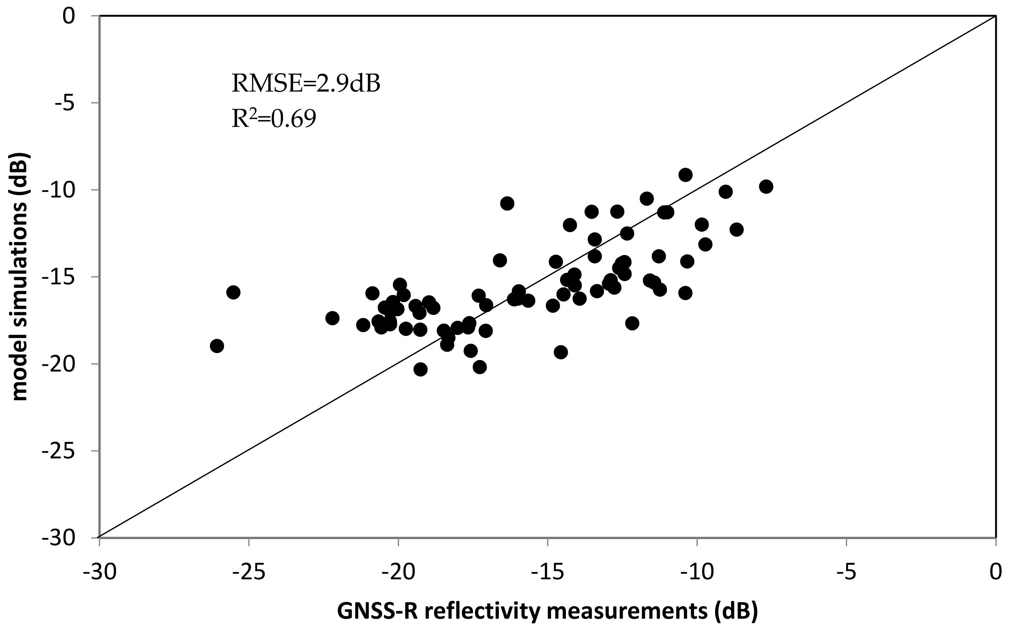
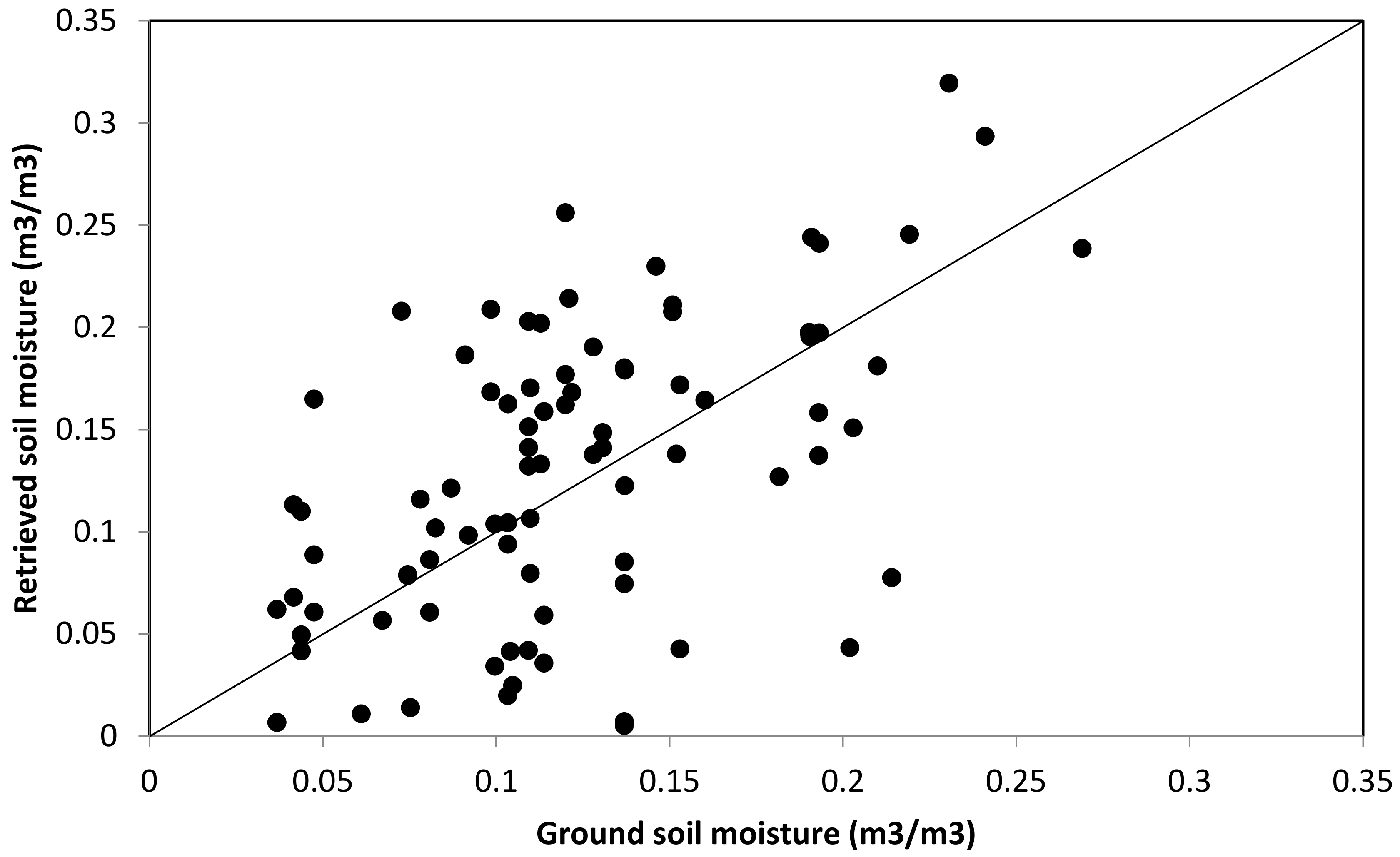
4. Modeling and Inversion of GNSS-R Reflectivity

In this section, the tau-omega model, which is used for microwave applications over continental surfaces [28,29], is applied to model GNSS-R reflectivity in an effort to improve our analysis and understand its behavior. This semi-empirical model is widely used over soil with vegetation cover because it is easily performed in an inversion scheme to estimate soil moisture and vegetation parameters.

4.1. Modeling of GNSS-R Reflectivity

The tau-omega model is used to model the vegetated soil reflectivity as [35,36]:

$${\Gamma }_p^{soil + vegetation}\left(\theta \right)={\Gamma }_p^{soil}\left(\theta \right).e^{-2{\tau }_p^{canopy}/\sin \theta }{\left(1-{\omega }_p^{canopy}\right)}^2$$

(5)

where ${\Gamma }_p$ is the reflection coefficient for circularly polarized (p) radiation, $2{\tau }_p^{canopy}$ is the two-way vegetation opacity, ${\left(1-{\omega }_p^{canopy}\right)}^2$ accounts for the two-way path of the GNSS signal, $\theta$ is the elevation angle and ${\omega }_p^{canopy}$ is the single scattering albedo.

In the case of low-lying vegetation, different studies have proposed linear relationships between the optical thickness and various vegetation parameters (LAI, vegetation water content) [26,27]. In the present study, we use the LAI parameter as a linear proxy for the optical thickness:

$${\tau }_p=a·LAI.$$

(6)

where a is a constant applied to all vegetation cover.

At the L-band, since the single-scattering albedo can be neglected for low vegetation cover development [35], Equation (5) can be simplified to:

$${\Gamma }_p\left(\theta \right)={\Gamma }_p^{soil}\left(\theta \right)·e^{-2a.LAI/\sin \theta }$$

(7)

When a logarithmic scale is applied, several studies have revealed a linear relationship between ${\Gamma }_p^{soil}$ and the soil moisture (Mv). As this behavior is also observed in the present study, we consider the approximation:

$${\Gamma }_{RL}^{soil}{\left(\theta \right)}_{dB}=\alpha Mv+\delta$$

(8)

Therefore, by applying a logarithmic function to Equation (7), we can write:

$${\Gamma }_p{\left(\theta \right)}_{dB}=\alpha Mv+\frac{\beta LAI}{sin\left(\theta \right)}+\delta$$

(9)

where α is the sensitivity of the reflectivity to soil moisture, β is the sensitivity of the reflectivity to the vegetation LAI, and δ is a constant related to the roughness effect. α, β and δ are empirical parameters retrieved from the experimental data. The parameters α, β and δ are estimated by minimizing the sum of the squared differences between the simulated and measured ${\Gamma }_{RL}$ data.

4.2. Application to the GLORI Data

The proposed model was applied to the reflectivity ${\Gamma }_{RL}$, derived from data recorded at all elevations between 50° and 90°. To evaluate the model linking ${\Gamma }_{RL}$ to soil moisture and LAI, we implemented a 5-fold cross-validation approach. Our database set (90 samples, each of which corresponds to a GNSS-R mean measurement on a reference field and a given date) was divided into five disjoint folds of the same size. In these sequential folds, the first was used for validation, and the four remaining folds were used for model parameterization. As in the case of the “repeated holdout” method, the overall accuracy is given by the average of the values obtained from all runs.

The calibrated parameters α, β, and δ can then be introduced into Equation (9), together with the known values of soil moisture, vegetation LAI and elevation angle, to determine the expected GNSS-R reflectivity.

The retrieved equation is written as:

$${\Gamma }_p{\left(\theta \right)}_{dB}=40.73 Mv-\frac{0.421 LAI}{\sin \left(\theta \right)}-19.04$$

(10)

where Mv is the soil moisture in (m³/m³).

Figure 7 illustrates the comparison between the observed and modeled reflectivity over the training dataset. The determinant coefficient R² is 0.69, with an RMSE (root mean square error) equal to 2.9 dB. The points showing the highest discrepancy with the proposed model correspond to the corn reference fields having the highest vegetation height. The use of LAI as a proxy for optical thickness instead of vegetation water content induces some limitations related to the saturation of LAI for dense or high covers.

If we consider the known ${\Gamma }_{RL}$ reflectivity and the LAI, we can estimate the soil moisture values of the validation set by inverting Equation (10), and we obtain:

$$Mv=0.025 {\Gamma }_p{\left(\theta \right)}_{dB}+\frac{0.01 LAI}{\sin \left(\theta \right)}+0.47$$

(11)

Figure 8 illustrates the comparison between the estimated and measured in situ soil moisture. The results illustrate an RMSE equal to 0.06 m³/m³. This accuracy is in agreement with those retrieved by other studies using GNSS-R airborne measurements [20,21,22,23].

The results show that the tau-omega model has a high potential for the retrieval of the GNSS-R ${\Gamma }_{RL}$ reflectivity. The model is based on the combined contributions from only two parameters: soil moisture and vegetation LAI. The highest simulated values of ${\Gamma }_{RL}$ are retrieved for fields with a slight vegetation coverage (low LAI), in agreement with the observed signals. An increase in vegetation LAI leads to an increase in vegetation attenuation, thus decreasing the global simulated signal. When all types of vegetation are considered in the validation process, no large discrepancies are revealed between the different types of cover (Figure 7). It is interesting to note that a single set of parameters (α, β, δ) can be used for all types of vegetation cover (wheat, corn, etc.), from which it is possible to derive satisfactory results, with an RMSE equal to 2.9 dB and R² equal to 0.69 for simulation of GNSS-R reflectivity and only 0.06 m³/m³ as RMSE for the soil moisture inversion from the GNSS-R data. In the case of the present study, the dataset was too small to separately consider the vegetation covers with different parameterizations of the tau-omega model. However, in the context of its potential application to low-resolution satellite observations (with CYGNSS for example), these results could justify the use of just one variable (e.g., the NDVI) to describe the vegetation for all agricultural areas, with only one parameterization for the inversion model.

5. Conclusions

The aim of this study was to confirm the sensitivity of airborne GNSS-R measurements to soil moisture and vegetation parameters over agricultural crops. An extensive campaign was conducted with the GLORI instrument over two agricultural sites in the southwest of France, with collocated measurements of soil moisture and vegetation parameters. The sensitivity of the GNSS-R measurements to soil moisture content was evaluated through the interpretation of data corresponding to low and high LAI levels, ranging from bare soil to dense cover, and for two elevation intervals (50–70° and 70–90°). Three GNSS-R observables (right-left apparent reflectivity (${\Gamma }_{RL}$), the reflected signal noise ratio (SNR), and the polarimetric ratio (PR)) were found to increase with increasing soil moisture. The sensitivities of reflectivity ${\Gamma }_{RL}$ and reflected SNR to soil moisture were also found to increase with an increasing elevation angle, equal to 40 dB/(m³/m³) and 45.7 dB/(m³/m³) for the case of reflectivity and the two elevation intervals (50–70° and 70–90°), respectively. The third observable PR was weakly correlated to the soil moisture.

The role of vegetation on the GNSS-R observables dynamic was analyzed using a class of data with approximately the same soil moisture conditions (dry conditions with soil moisture lower than 0.1 m³/m³), revealing a sensitivity to the vegetation LAI, with a clear decrease in all GNSS-R observables with an increasing vegetation LAI. The correlations between the vegetation LAI and both ${\Gamma }_{RL}$ and the reflected signal SNR were strongest in the case of low elevation angles. The correlation was very weak for high elevation angles. The sensitivities of these observables were quite similar, equal to −0.91 dB/(m²/m²) and −0.76 dB/(m²/m²) for the case of elevation angle between 50° and 70°, respectively. The PR observable illustrates the high potential for vegetation LAI retrieval, probably due to the high effect of vegetation on GNSS data depolarization.

A simplified tau-omega model was proposed for modeling the ${\Gamma }_{RL}$, observed over reference plots as a function of soil moisture, LAI and elevation angle. Although several different types of plants were considered in this study, the proposed model demonstrated good potential for the simulation of ${\Gamma }_{RL}$ data, with RMSE equal to 2.9 dB and R² equal to 0.64 for GNSS-R data with elevation angles ranging between 50° and 90°. The validation step applied using a 5-fold cross-validation approach illustrated an RMSE equal to 0.06 m³/m³ between retrieved and ground soil moistures values. As the model was developed using data acquired during an airborne campaign over two study sites and applied to different vegetation covers, it is considered to be reliable and more broadly applicable to the interpretation of satellite GNSS-R data. Future studies will be designed to confirm these results through the measurement and interpretation of satellite GNSS-R signals observed with the TechDemoSat and CYGNSS satellites, and the proposed development of a retrieval algorithm based on the use of additional vegetation information, which is easily measurable from optical satellite sensors, such as the NDVI.

References

1. Koster, R.D.; Dirmeyer, P.A.; Guo, Z.; Bonan, G.; Chan, E.; Cox, P.; Gordon, C.T.; Kanae, S.; Kowalczyk, E.; Lawrence, D.; et al. Regions of Strong Coupling Between Soil Moisture and Precipitation. Science 2004, 305, 1138–1140. [Google Scholar] [CrossRef] [PubMed]
2. Manfreda, S.; Scanlon, T.M.; Caylor, K.K. On the importance of accurate depiction of infiltration processes on modelled soil moisture and vegetation water stress. Ecohydrology 2009, 3, 155–165. [Google Scholar] [CrossRef]
3. Saux-Picart, S.; Ottlé, C.; Decharme, B.; André, C.; Zribi, M.; Perrier, A.; Coudert, B.; Boulain, N.; Cappelaere, B. Water and Energy budgets simulation over the Niger super site spatially constrained with remote sensing data. J. Hdrol. 2009, 375, 287–295. [Google Scholar] [CrossRef]
4. Zhuo, L.; Han, D. The relevance of soil moisture by remote sensing and hydrological modelling. Procedia Eng. 2016, 154, 1368–1375. [Google Scholar] [CrossRef]
5. Fieuzal, R.; Duchemin, B.; Jarlan, L.; Zribi, M.; Baup, F.; Merlin, O.; Dedieu, G.; Garatuza-Payan, J.; Watt, C.; Chehbouni, A. Combined use of optical and radar satellite data for the monitoring of irrigation and soil moisture of wheat crops. Hydrol. Earth Syst. Sci. 2011, 15, 1117–1129. [Google Scholar] [CrossRef] [Green Version]
6. Paloscia, S.; Macelloni, G.; Santi, E. Soil Moisture Estimates from AMSR-E Brightness Temperatures by Using a Dual-Frequency Algorithm. IEEE Trans. Geosci. Remote Sens. 2006, 44, 3135–3144. [Google Scholar] [CrossRef]
7. Wagner, W.; Lemoine, G.; Rott, H. A Method for Estimating Soil Moisture from ERS Scatterometer and Soil Data. Remote Sens. Environ. 1999, 70, 191–207. [Google Scholar] [CrossRef]
8. Fernandez-Moran, R.; Al-Yaari, A.; Mialon, A.; Mahmoodi, A.; Al Bitar, A.; De Lannoy, G.; Rodriguez-Fernandez, N.; Lopez-Baeza, E.; Kerr, Y.; Wigneron, J.P. SMOS-IC: An alternative SMOS soil moisture and vegetation optical depth product. Remote Sens. 2017, 9, 457. [Google Scholar] [CrossRef]
9. Rodríguez-Fernández, N.J.; Aires, F.; Richaume, F.; Kerr, Y.H.; Prigent, C.; Kolassa, J.; Cabot, F.; Jiménez, C.; Mahmoodi, A.; Drusch, M. Soil moisture retrieval using neural networks: Application to SMOS. IEEE Trans. Geosci. Remote Sens. 2015, 53, 5991–6007. [Google Scholar] [CrossRef]
10. Fratanellli, G.; Paloscia, S.; Zribi, M.; Chahbi, A. Sensitivity analysis of X-band SAR to wheat and barley biomass in the Merguellil Basin. Remote Sens. Lett. 2013, 4, 1107–1116. [Google Scholar] [CrossRef]
11. Zribi, M.; Gorrab, A.; Baghdadi, N. A new soil roughness parameter for the modelling of radar backscattering over bare soil. Remote Sens. Environ. 2014, 152, 62–73. [Google Scholar] [CrossRef] [Green Version]
12. Tomer, S.K.; Al Bitar, A.; Sekhar, M.; Corgne, S.; Bandyopadhyay, S.; Sreelash, K.; Sharma, A.K.; Zribi, M.; Kerr, Y. Retrieval and Multi-scale Validation of Soil Moisture from Multi-temporal SAR Data in a Tropical Region. Remote Sens. 2015, 7, 8128–8153. [Google Scholar] [CrossRef]
13. Martin-Neira, M. A Passive Reflectometry and Interferometry System(PARIS): Application to Ocean Altimetry. ESA J. 1993, 17, 331–355. [Google Scholar]
14. Zavorotny, V.U.; Gleason, S.; Cardellach, E.; Camps, A. Tutorial on Remote Sensing Using GNSS Bistatic Radar of Opportunity. IEEE Geosci. Remote Sens. Mag. 2014, 2, 8–45. [Google Scholar] [CrossRef] [Green Version]
15. Masters, D.; Axelrad, P.; Katzberg, S. Initial results of land-reflected GPS bistatic radar measurements in SMEX02. Remote Sens. Environ. 2004, 92, 507–520. [Google Scholar] [CrossRef]
16. Egido, A.; Caparrini, M.; Ruffini, G.; Paloscia, S.; Santi, E.; Guerriero, L.; Pierdicca, N.; Floury, N. Global navigation satellite systems reflectometry as a remote sensing tool for agriculture. Remote Sens. 2012, 4, 2356–2372. [Google Scholar] [CrossRef]
17. Paloscia, S.; Santi, E.; Fontanelli, G.; Pettinato, S.; Egido, A.; Caparrini, M.; Motte, E.; Guerriero, L.; Pierdicca, N.; Floury, N. Grass: AN experiment on the capability of airborne GNSS-R sensors in sensing soil moisture and vegetation biomass. In Proceedings of the 2013 IEEE International Geoscience and Remote Sensing Symposium-IGARSS, Melbourne, Australia, 21–26 July 2013; pp. 2110–2113. [Google Scholar]
18. Sánchez, N.; Alonso-Arroyo, A.; Martínez-Fernández, J.; Piles, M.; González-Zamora, A.; Camps, A.; Vall-llosera, M. On the Synergy of Airborne GNSS-R and Landsat 8 for Soil Moisture Estimation. Remote Sens. 2015, 7, 9954–9974. [Google Scholar] [CrossRef] [Green Version]
19. Camps, A.; Park, H.; Pablos, M.; Foti, G.; Gommenginger, C.P.; Liu, P.W.; Judge, J. Sensitivity of GNSS-R Spaceborne Observations to Soil Moisture and Vegetation. IEEE J. Sel. Top. Appl. Earth Obs. Remote Sens. 2016, 9, 4730–4742. [Google Scholar] [CrossRef] [Green Version]
20. Pei, Y.; Notarpietro, R.; Savi, P.; Cucca, M.; Dovis, F. A fully software Global Navigation Satellite System reflectometry (GNSS-R) receiver for soil monitoring. Int. J. Remote Sens. 2014, 35, 2378–2391. [Google Scholar]
21. Jia, Y.; Savi, P. Estimation of Surface Characteristics Using GNSS LH Reflected Signals: Land versus Water. IEEE J. Sel. Top. Appl. Earth Obs. Remote Sens. 2016, 9, 4752–4758. [Google Scholar] [CrossRef]
22. Katzberg, S.J.; Torres, O.; Grant, M.S.; Masters, D. Utilizing calibrated GPS reflected signals to estimate soil reflectivity and dielectric constant: Results from SMEX02. Remote Sens. Environ. 2006, 100, 17–28. [Google Scholar] [CrossRef] [Green Version]
23. Rodriguez-Alvarez, N.; Bosch-Lluis, X.; Camps, A.; Vall-llossera, M.; Valencia, E.; Marchan-Hernandez, J.F.; Ramos-Perez, I. Soil moisture retrievals using GNSS-R techniques: Experimental Results over a Bare Soil Field. IEEE Trans. Geosci. Remote Sens. 2009, 47, 3616–3624. [Google Scholar] [CrossRef]
24. Jia, Y.; Savi, P. Sensing soil moisture and vegetation using GNSS-R polarimetric measurement. Adv. Space Res. 2017, 59, 858–869. [Google Scholar] [CrossRef]
25. Egido, A. GNSS Reflectometry for Land Remote Sensing Applications. Ph.D. Thesis, Universitat Politècnica de Catalunya, Barcelona, Spain, July 2013. [Google Scholar]
26. Egido, A.; Paloscia, S.; Motte, E.; Guerriero, L.; Pierdicca, N.; Caparrini, M.; Santi, E.; Fontanelli, G.; Floury, N. Airborne GNSS-R Polarimetric Measurements for Soil Moisture and Above-Ground Biomass Estimation. IEEE J. Sel. Top. Appl. Earth Obs. Remote Sens. 2014, 7, 1522–1532. [Google Scholar] [CrossRef]
27. Unwin, M.; Blunt, P.; de Vos van Steenwijk, R.; Duncan, S.; Martin, G.; Jales, P. GNSS Remote Sensing and Technology Demonstration on TechDemoSat-1. In Proceedings of the 24th International Technical Meeting of The Satellite Division of the Institute of Navigation (ION GNSS 2011), Portland, OR, USA, 20–23 September 2011; pp. 2970–2975. [Google Scholar]
28. Chew, C.; Shah, R.; Zuffada, C.; Hajj, G.; Masters, D.; Mannucci, A.J. Demonstrating soil moisture remote sensing with observations from the UK TechDemoSat-1 satellite mission. Geophys. Res. Lett. 2016, 43, 3317–3324. [Google Scholar] [CrossRef]
29. Carreno-Luengo, H.; Lowe, C.; Zuffada, S.; Esterhuizen, S.; Oveisgharan, S. Spaceborne GNSS-R from the SMAP mission: first assessment of polarimetric scatterometry over land and cryosphere. Remote Sens. 2017, 9, 326. [Google Scholar] [CrossRef]
30. Motte, E.; Zribi, M.; Fanise, P.; Egido, A.; Darrozes, J.; Al-Yaari, A.; Baghdadi, N.; Baup, F.; Dayau, S.; Fieuzal, R.; et al. GLORI: A GNSS-R Dual Polarization Airborne Instrument for Land Surface Monitoring. Sensors 2016, 16, 732. [Google Scholar] [CrossRef] [PubMed] [Green Version]
31. Lestarquit, L.; Peyrezabes, M.; Darrozes, J.; Motte, E.; Roussel, N.; Wautelet, G.; Frappart, F.; Ramillien, G.; Biancale, R.; Zribi, M. Reflectometry with an open-source Software GNSS receiver. Application Case with Carrier Phase Altimetry. IEEE J. Sel. Top. Appl. Earth Obs. Remote Sens. 2016, 9, 4843–4853. [Google Scholar] [CrossRef]
32. Motte, E.; Zribi, M. Optimizing waveform maximum determination for specular point tracking in airborne GNSS-R. Sensors 2017, 17, 1880. [Google Scholar] [CrossRef] [PubMed]
33. Gueeriero, L.; Pierdicca, N.; Pulvirenti, L.; Ferrazzoli, P. Use of satellite radar bistatic measurements for crop monitoring: A simulation study on corn field. Remote Sens. 2013, 5, 864–890. [Google Scholar] [CrossRef]
34. Pierdicca, N.; Guerriero, L.; Giusto, R.; Brogioni, M.; Egido, A. SAVERS: A Simulator of GNSS Reflections from Bare and Vegetated Soils. IEEE Trans. Geosci. Remote Sens. 2014, 52, 6542–6554. [Google Scholar] [CrossRef]
35. Ulaby, F.T.; Moore, R.K.; Fung, A.K. Microwave Remote Sensing: Active and Passive-Volume 1-Microwave Remote Sensing Fundamentals and Radiometry. 1981. Available online: https://fdbktgsmn.updog.co/ZmRia3Rnc21uMDIwMTEwNzU5Nw.pdf (accessed on 6 July 2018).
36. Jackson, T.J.; Schmugge, T.J.; Wang, J.R. Passive microwave moisture sensing of soil under vegetation canopies. Water Resour. Res. 1982, 18, 1137–1142. [Google Scholar] [CrossRef]
Figure 1. GLORI’2015 flight plan and ground truth collection zones.
Remotesensing 10 01245 g001
Figure 2. Reference field locations. (a) Lamasquère site (background: Landsat image on 28 June 2015), (b) Marcheprime site (background: Landsat image on 3 July 2015).
Remotesensing 10 01245 g002
Figure 3. Global Navigation Satellite System reflectometry (GNSS-R) observables at 50–70° elevation angles as a function of soil moisture: (a) cross-polarization (right-left) reflectivity ( Γ R L ) for leaf area index (LAI) < 1; (b) signal-to-noise ratio (SNR) for LAI < 1; (c) polarimetric ratio (PR) for LAI < 1; (d) Γ R L for LAI > 1; (e) SNR for LAI > 1; (f) PR for LAI > 1.
Remotesensing 10 01245 g003aRemotesensing 10 01245 g003b
Figure 4. GNSS-R observables at 70–90° elevation angles as a function of soil moisture: (a) Γ R L for LAI < 1; (b) SNR for LAI < 1; (c) PR for LAI < 1; (d) Γ R L for LAI > 1; (e) SNR for LAI > 1; (f) PR for LAI > 1.
Remotesensing 10 01245 g004aRemotesensing 10 01245 g004b
Figure 5. GNSS-R observables at 50–70° elevation angles as a function of LAI at dry conditions (wet moisture values (Mv) < 0.1 m3/m3): (a) Γ R L ; (b) SNR; (c) PR.
Remotesensing 10 01245 g005
Figure 6. GNSS-R observables at 70–90° elevation angles as a function of LAI at dry conditions (Mv < 0.1 m3/m3): (a) Γ R L ; (b) SNR; (c) PR.
Remotesensing 10 01245 g006
Figure 7. Modeled vs observed Γ R L using the training dataset. RMSE = root mean square error.
Remotesensing 10 01245 g007
Figure 8. Comparison between the retrieved soil moisture from Γ R L and ground soil moisture measurements.
Remotesensing 10 01245 g008