Accelerated RAPID Model Using Heterogeneous Porous Objects

Abstract

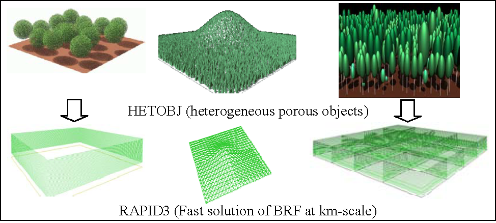
To enhance the capability of three-dimensional (3D) radiative transfer models at the kilometer scale (km-scale), the radiosity applicable to porous individual objects (RAPID) model has been upgraded to RAPID3. The major innovation is that the homogeneous porous object concept (HOMOBJ) used for a tree crown scale is extended to a heterogeneous porous object (HETOBJ) for a forest plot scale. Correspondingly, the radiosity-graphics-combined method has been extended from HOMOBJ to HETOBJ, including the random dynamic projection algorithm, the updated modules of view factors, the single scattering estimation, the multiple scattering solutions, and the bidirectional reflectance factor (BRF) calculations. Five cases of the third radiation transfer model intercomparison (RAMI-3) have been used to verify RAPID3 by the RAMI-3 online checker. Seven scenes with different degrees of topography (valleys and hills) at 500 m size have also been simulated. Using a personal computer (CPU 2.5 GHz, memory 4 GB), the computation time of BRF at 500 m is only approximately 13 min per scene. The mean root mean square error is 0.015. RAPID3 simulated the enhanced contrast of BRF between backward and forward directions due to topography. RAPID3 has been integrated into the free RAPID platform, which should be very useful for the remote sensing community. In addition, the HETOBJ concept may also be useful for the speedup of ray tracing models.

1. Introduction

Modeling radiative transfer (RT) of vegetation is a fundamental problem of land surface remote sensing. The bidirectional reflectance distribution function (BRDF) is one of the most important outputs for RT models, which can help normalize directional reflectance to more consistent nadir BRDF-adjusted surface reflectances (NBAR) products [1,2] or extract vegetation information [3]. However, natural vegetation generally has significant spatial heterogeneity in both horizontal and vertical dimensions [4], resulting in a great challenge to retrieve an accurate vegetation leaf area index (LAI) and cover fraction [5,6]. In mountainous areas, it is much more complex due to the three-dimensional (3D) structure of forest vegetation and terrain background [7]. To our knowledge, there are only two widely used operational BRDF products, MCD43 of the moderate resolution imaging spectroradiometer (MODIS) [2,8] and the multiangle imaging spectroradiometer (MISR). Both have a spatial resolution of 500 m or 1 km. Within a domain with a size larger than 0.5 km (hereafter named the km-scale), the land surface is more likely to be heterogeneous with changing elevations or mixed land covers. Especially in mountainous areas, forest BRDF and albedo are significantly affected by the heterogeneous terrain and complex vegetation composition [9,10]. To simulate the combined effects of heterogeneous terrain and complex vegetation composition on MODIS or MISR BRDF products, RT models are expected to contend with a domain (or scene) size greater than 0.5 km. Although many 3D models may simulate such a large scene, there are very few that are specifically optimized to cope with the km-scale. Thus, a suitable RT model at the km-scale considering heterogeneous terrain is strongly required to deeply understand the RT process and improve the inversion accuracy of LAI and the vegetation cover fraction.

Considering the 3D nature of forest heterogeneities, there are three potential groups of RT models to be used at the km-scale: (a) the modified geometric optical reflectance models (GO) [7,11]; (b) classical 3D radiative transfer (3DRT) solutions [12,13]; (c) computer simulation models using ray tracing [14,15] or radiosity techniques [16]. GO models, usually used for a flat background [11,17], have been improved recently on an inclined slope [7]. However, it is still difficult to extend GO models to larger scales containing more than one slope. The 3DRT models have good mathematics and physical background, but they also have a weakness in describing the topography effect (nonflat terrain), as well as the multiple scattering processes that occur within the minimum 3D element (cells or voxels). Another limitation of 3DRT is its time-consuming feature arising from the equally defined discrete directions. The GO models have a key role in describing generalized BRDF features, and can simulate canopy reflectance reasonably well in many cases. However, they are also heavily reliant on the validity of various sets of assumptions and simplifications, and thus, are limited to relatively simple heterogeneous scenes on flat or constant slope terrains. The 3DRT models are attractive in their use of a Cartesian grid of volume cells (voxels) that reduce scene complexity but maintain a certain degree of spatial fidelity. However, there will be an inherent loss of the structural heterogeneity within the voxel resulting from averaging canopy structural properties. By contrast, computer simulation models have fewer assumptions on topography and tree structure, and have more suitability for scientific research, and are thus widely used to support sensor design [18], model validation [19], and assumption evaluation [20,21].

However, complaints of computer simulation models (both ray tracing and radiosity) have also been discussed because of their low computation efficiency from considering too much of the 3D details in the explicit descriptions of location, orientation, size, and shape of each scatterer. This limitation may hamper their expansion at the km-scale. To reduce the computation cost, a few efforts have been made recently to develop faster computer simulation models. For example, the discrete anisotropic radiative transfer (DART) model used balanced voxel size and improved its direction discretization and oversampling algorithms [22]. The Rayspread model [23] used the message passing interface (MPI) to construct a distributed and parallel simulation architecture and accelerate the Raytran code [15]. To simulate realistic 3D scenes at the km-scale, the large-scale emulation system for realistic three-dimensional forest simulation (LESS) model also used parallel computation to accelerate the ray tracing code [24]. Based on the radiosity-graphics-combined model (RGM) [25], a subdivision method was adopted to simulate directional reflectance over a 500 m forest scene containing topography [26]. By defining the concept of “porous object”, the radiosity applicable to a porous individual objects (RAPID) model significantly reduced the 3D scene complexity and improved the computation efficiency on directional reflectance [16,27].

However, most computer simulation models still focused on domain sizes less than 500 m [19]. The km-scale RT models are very limited. These km-scale RT models, such as the LESS model [24], are usually running on supercomputers in the laboratory to save time, which is not a convenient approach for widespread use. Desktop computers are generally inexpensive and are easier to access than supercomputers. It will be beneficial for scientists to use desktop computers if any 3D model can be identified that runs fast at the km-scale on a desktop platform with comparable accuracy to models run on supercomputers. As a result, more remote sensing users can conduct their desired simulations easily, such as assessing topographic correction accuracy [28,29], testing scale effects [30] or validating large-scale BRDF models over complex terrains [31]. Furthermore, from the completeness aspect of the RT family, km-scale models are also important to fill the missing part of the landscape scale.

With these considerations in mind, the porous object concept is upgraded from RAPID at the tree crown scale to the heterogeneous porous object at the plot scale to accelerate RAPID for km-scale scenes, hereafter called RAPID3 version. Section 2 introduces the history and background of radiosity and RAPID. Then, the extension method of RAPID3 on km-scale simulation is presented in Section 3. The next section evaluates RAPID3 using the third radiation transfer model intercomparison (RAMI-3) test cases. Finally, the conclusion and future remarks comprise Section 5.

2. Theoretical Background of RAPID

RAPID is a radiosity-based model using computer graphics methods to compute RT within and above 3D vegetated scenes from visible/near infrared (VNIR, 0.47–2.5 μm) [16] to thermal infrared (TIR, 8–14 μm) [32], and microwave (MV, 2.5–30 cm) parts [33] of the electromagnetic spectrum [16,33].

The traditional radiosity methods [32] use planar surfaces to create the 3D scene and solve the RT in VNIR and TIR as follows:

$$B_i=E_i+{\chi }_i{\displaystyle \sum F_{ij}{B}_j}i,j=1,2,\dots 2N,$$

(1)

where

$${\chi }_i=\left\{\begin{array}{l}{\rho }_i,\mathbf{if}\left({\stackrel{\rightharpoonup }{n}}_i\cdot {\stackrel{\rightharpoonup }{n}}_j\right)<0\\ {\tau }_i,\mathbf{if}\left({\stackrel{\rightharpoonup }{n}}_i\cdot {\stackrel{\rightharpoonup }{n}}_j\right)>0\end{array}\right\}.$$

(2)

B_i or B_j is the radiosity on surface element i or j, defined as the total radiation flux density leaving that surface (the unit is Wm⁻²). E_i is the surface thermal emission in TIR or the light source emission in VNIR, and χ_i is the surface reflection or transmission coefficient which depends on the relative orientation (normal vector $\stackrel{\rightharpoonup }{n}$) of surface i and j to each other. The F_ij is the form factor or “view factor” which specifies the fraction of radiant flux leaving another surface j that reaches the surface i, and N is the number of discrete two-sided surface elements to be considered.

Equation (1) works well at small scales (e.g., crop canopies at a small domain size) with a few planar surfaces. However, a 3D scene at large scales (e.g., forest canopies at a large domain size) could have millions of surfaces, resulting in a huge memory burden and high computation time cost on computers. For example, the radiosity-graphics-based model (RGM) [25] may crash if the surface polygon number is larger than 500,000 on a 32 bit operation system (OS). To reduce the limitation, RGM was extended to large-scale forest canopies using a subscene division method [26]. This version has been verified in the context of the fourth RAMI (RAMI-IV) (marked as RGM2). To save time, parallel computation of subscenes was implemented using a few personal computers (PC). However, one subscene failure due to unexpected bugs would lead to the failure to merge the whole scene, which is still not ideal for users.

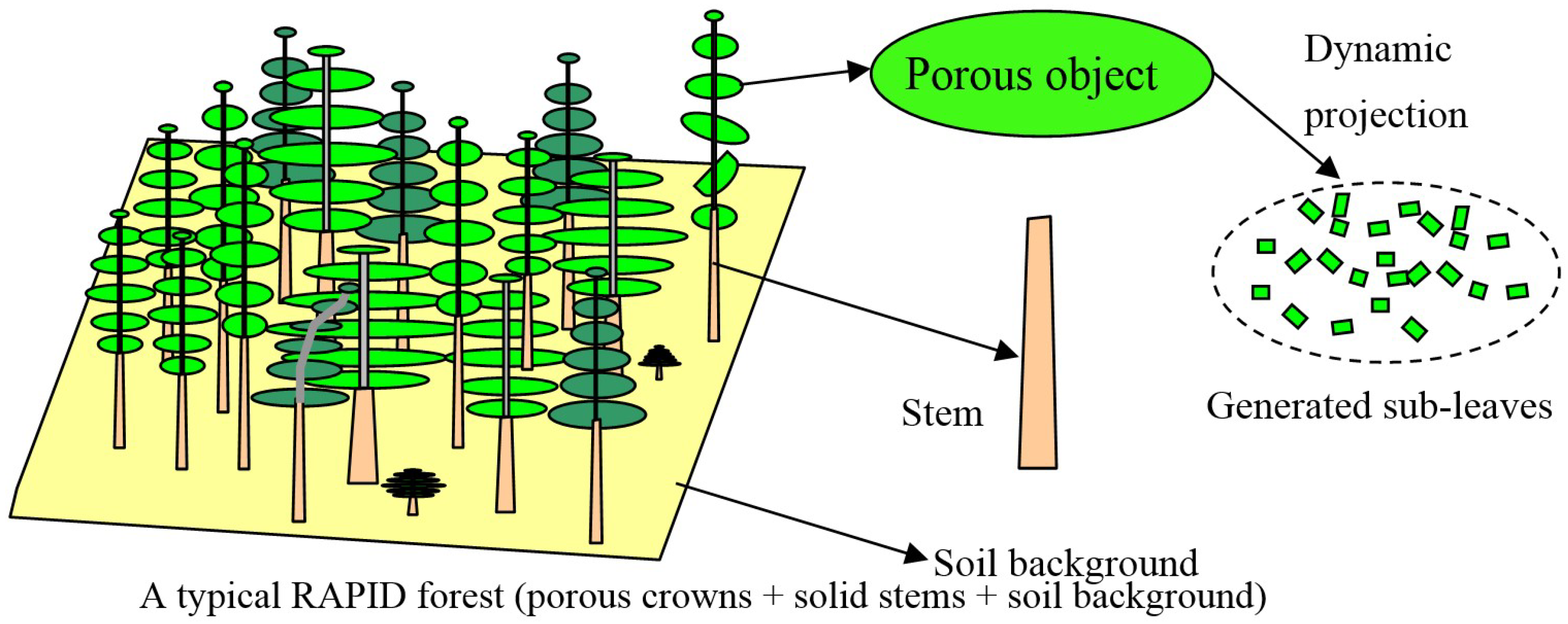
Thus, RAPID was developed based on RGM for large-scale forest scenes, which is considerably easier to use and faster than RGM2. RAPID is capable of simulating the bidirectional reflectance factor (BRF) over various kinds of vegetated scenes (homogeneous or heterogeneous). Unlike the thousands of polygons used in RGM2, RAPID uses dozens of porous objects to represent a group of grass or crop plants or tree crowns (see Figure 1). Each porous object has several properties, including shape, size, thickness, LAI, leaf angle distribution (LAD), and leaf clumping conditions. These properties are used during dynamical generation of the subleaves within porous objects at run-time; hence, only view factors between porous objects (not between hundreds of small leaves) need to be calculated and stored. As a result, the model significantly reduces the huge memory requirement and long computation time of view factors for a large and realistic vegetation scene.

Seven major steps are required for RAPID to simulate the BRF:

(1) Generating a user-defined 3D scene containing porous objects using the graphical user interface (GUI) developed via C++ language, and an open graphic library (OpenGL) based on the digital elevation model (DEM), and a reference background picture and forest inventory data as inputs. Users can freely define 3D objects (tree species, crop types, buildings, and water bodies) and place them on the target regions. A parameter editor is integrated in the GUI to modify the key parameters, such as height, width, orientation, radius, and so on.

(2) Calculating sunlit fractions and irradiances from direct light of all objects using the painter algorithm, and a dynamic projection method in the solar incident direction is performed. The painter algorithm sorts all the objects in a scene by their depths to the painter and then paints them in this order. The dynamic projection generates randomly oriented and located leaves within a porous object according to its properties, including LAI, LAD, and leaf size.

(3) Calculating view fractions of sky and irradiances from diffuse light of all objects by averaging those from a few solid angles (at least 40) of the above sky (hemisphere) is performed. In each solid angle, the dynamic projection similar to (2) is used. During the dynamic projections, the overlapping fractions between any pairs of objects are recorded.

(4) Estimating view factors between all pairs of objects using their mean overlapping fractions in all solid angles, as described in step (3), is performed.

(5) Determining single scattering values of all objects using the direct irradiance results from step (2) and diffuse irradiance from step (3) is performed. The equivalent reflectance and transmittance of porous objects are also estimated from leaf reflectance and transmittance using LAD.

(6) Solving multiple scattering and finding the best radiosity values using results of (4) and (5) is performed.

(7) Calculating BRFs and rendering images in all view directions is performed. At this step, the dynamic projection repeats for each view direction. However, to decide whether a pixel is sunlit or not, the projected image in (2) is required.

The results from all steps, including the generated 3D scene, direct light fractions and output radiosity values, can be rendered as gray or color images in arbitrary view directions in the GUI.

In 2016, RAPID2 [33] was released, including new functions of atmospheric RT by linking the vector linearized discrete ordinate radiative transfer (V-LIDORT) model [34], DBT simulation in TIR by updating TRGM code [35] and backscattering simulation in MV [36], as well as LiDAR point cloud and waveform simulations [37]. RAPID2 has been used to support comparing LAI inversion algorithms [38], validating a new kernel-based BRDF model [39], validating an analytic vegetation-soil-road-mixed DBT model [40], and simulating continuous remote sensing images [27]. Although RAPID2 is able to simulate km-scale images, it requires a few hours to run on a server (12 CPU cores), which may restrict RAPID2 to limited user groups having access to super computation power. Thus, the faster version RAPID3 is developed in this paper to specifically accelerate the simulation for km-scale scenes.

3. Model Description

RAPID3 is a downward compatible model of RGM, RAPID, and RAPID2. That means the RAPID model series can run at small scales with a few meters to large scales with kilometers. For clarity, the most suitable model at three scales was suggested to run efficiently:

• Small scenes of approximately a few meters: it is better to choose RGM using realistic leaves and branches as the basic elements;
• Middle scenes of approximately tens of meters: it is better to choose RAPID or RAPID2 using porous objects as the basic elements;
• Large scenes with hundreds of meters to kilometers (km-scale): it is better to choose a new version specified for this scale, e.g., the RAPID3 which is fully illustrated in this paper.

The focus of this paper is to develop RAPID3 for the km-scale.

3.1. Definition of the Heterogeneous Porous Object (HETOBJ)

In RAPID, a porous object is used to represent a thin layer of leaves with a low LAI (from 0.30 to 0.40 m²m⁻²) and a predefined LAD. The leaves are randomly distributed in the layer without significant clumping. Therefore, this porous object can be seen as a homogeneous porous object (HOMOBJ). HOMOBJ is good to describe a tree crown layer but not sufficient to define a layer of a forest plot. If users group several HOMOBJs into one porous object, the total object number in the 3D scene will be further reduced. As a result, the computation costs will also be reduced. This grouping of HOMOBJ is the key idea for RAPID3 to simulate km-scale scene rapidly, which is named as “heterogeneous porous objects” (HETOBJ). To be precise, a HETOBJ is an object representing a thin layer of leaves or trunks with significant horizontal clumping. A HETOBJ can be seen as a collection of HOMOBJs.

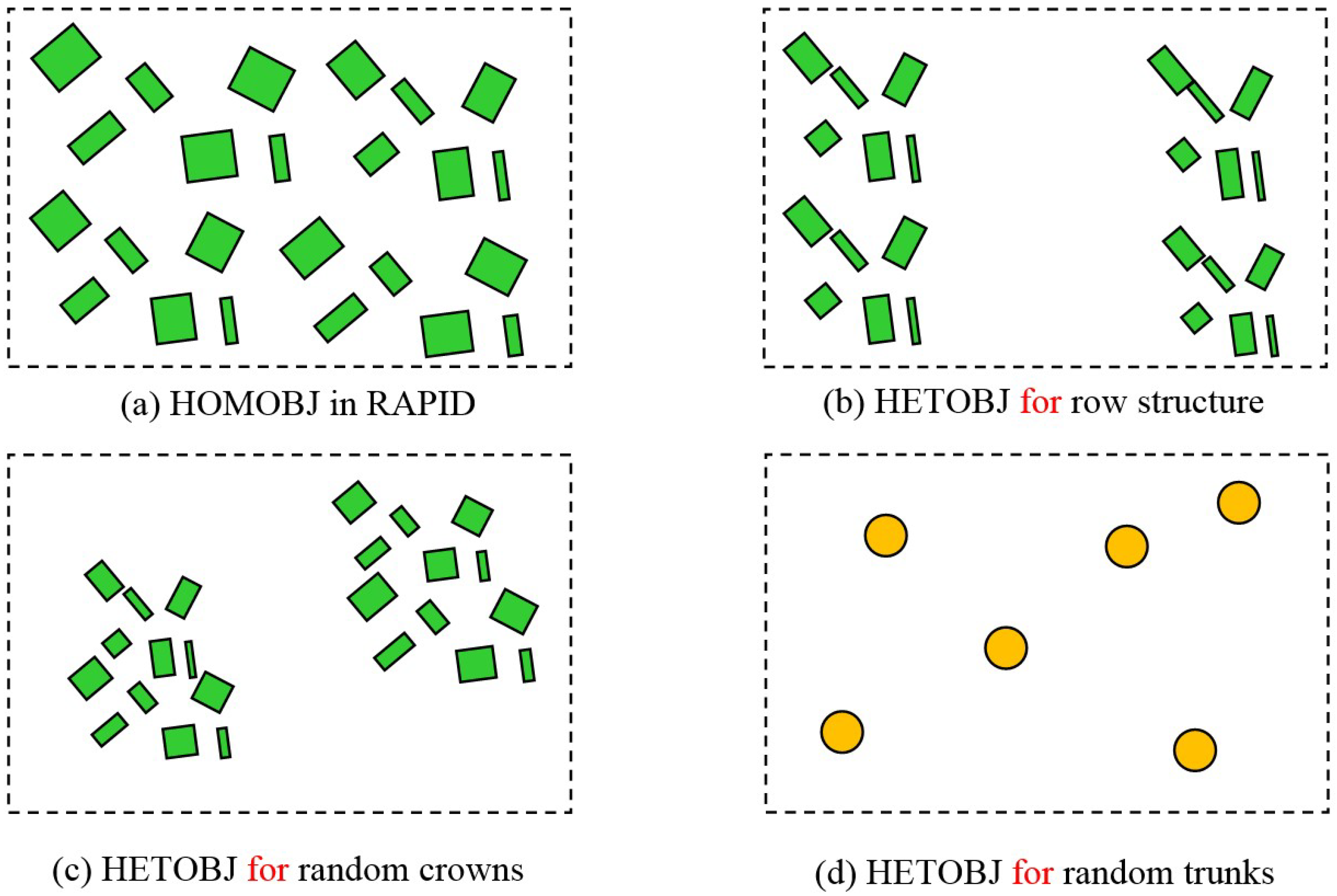
Figure 2 demonstrates the concepts of HOMOBJ and HETOBJ. The major feature of HOMOBJ is the simple random distribution of leaves in it. After extension, the leaves can be heterogeneously clumped in HETOBJ, such as the row structure (Figure 2b), clustering crowns (Figure 2c), and random trunk layers (Figure 2d). To describe the clumping effect in each HETOBJ, the number of clusters and the relative XY coordinates to the lower-left corner, as well as the shape and size of each cluster (e.g., the radius of a circular cluster for trees) should be given as input. Other major input parameters include LAI, LAD, crown thickness (h_crown) or trunk length (h_trunk), and leaf length (l).

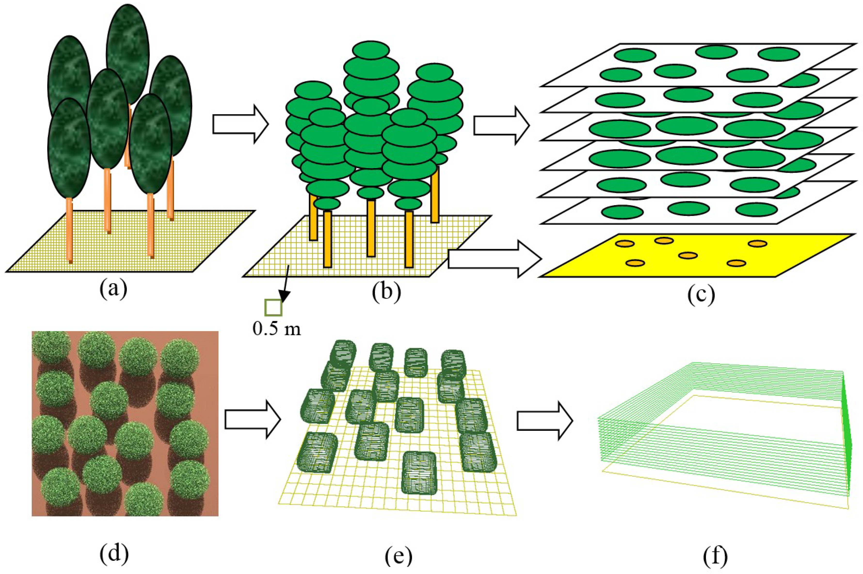
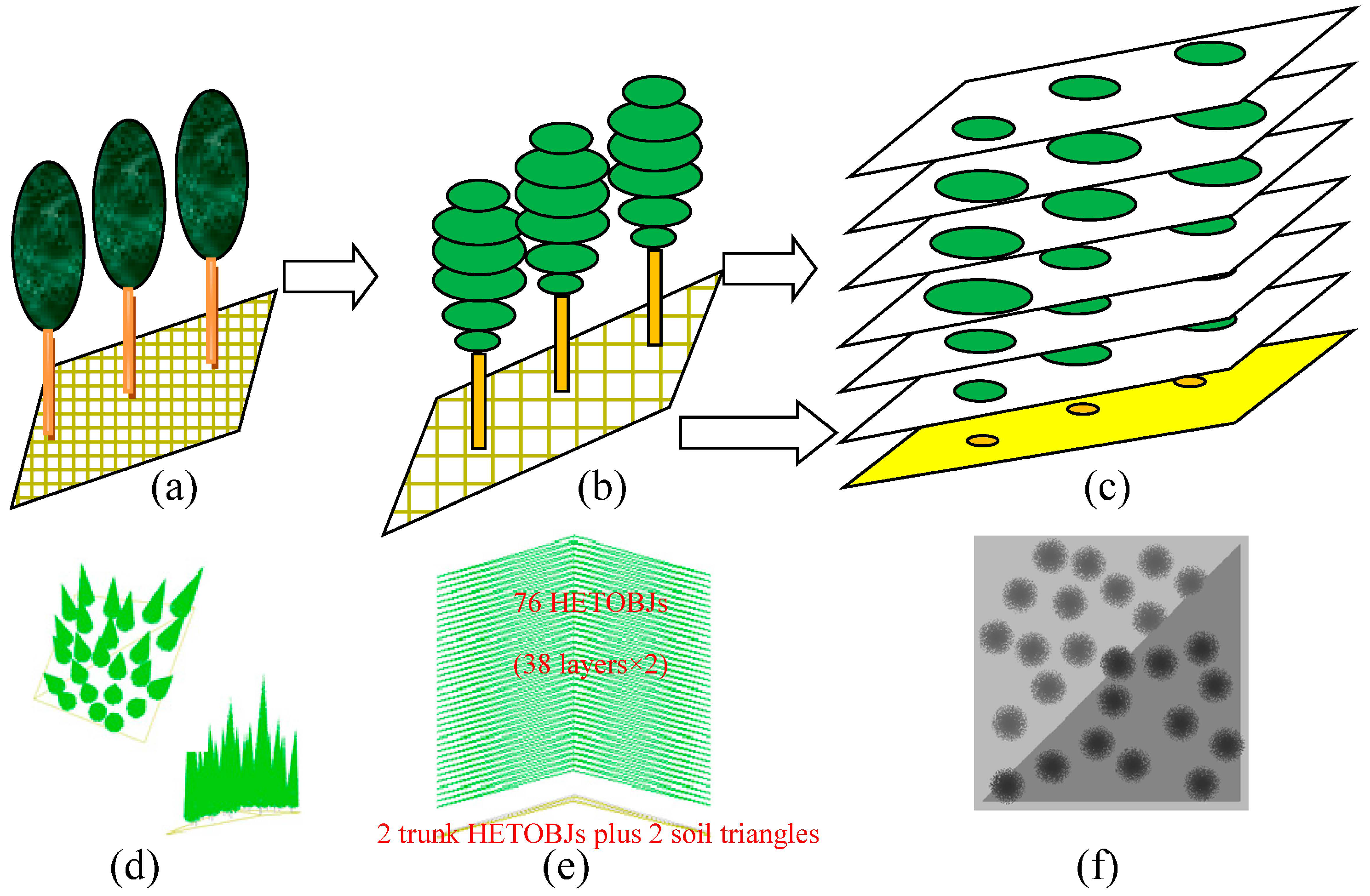
Figure 3 shows the examples of simplifying real-world forests (a and d) into the HOMOBJ in RAPID (b and e), and then into HETOBJ in RAPID3 (c and f). In Figure 3b, RAPID uses six HOMOBJs and one trunk to represent one tree, resulting in 36 HOMOBJs and six trunks. In Figure 3c, the scene is further simplified as the collection of six crowns and one trunk HETOBJ. The soil polygons are kept solid in both RAPID and RAPID3. In RAPID, the soil polygon size should not be too large (the default 0.5 m, Figure 3b) to achieve a good accuracy. However, in Figure 3c, one soil polygon is sufficiently the same size as the HETOBJ. Finally, there are only 7 HETOBJs in Figure 3c. Similarly, the forest stand containing 15 trees in Figure 3d was represented by 300 HOMOBJs in Figure 3e, which was then further simplified as only 20 HETOBJs in Figure 3f.

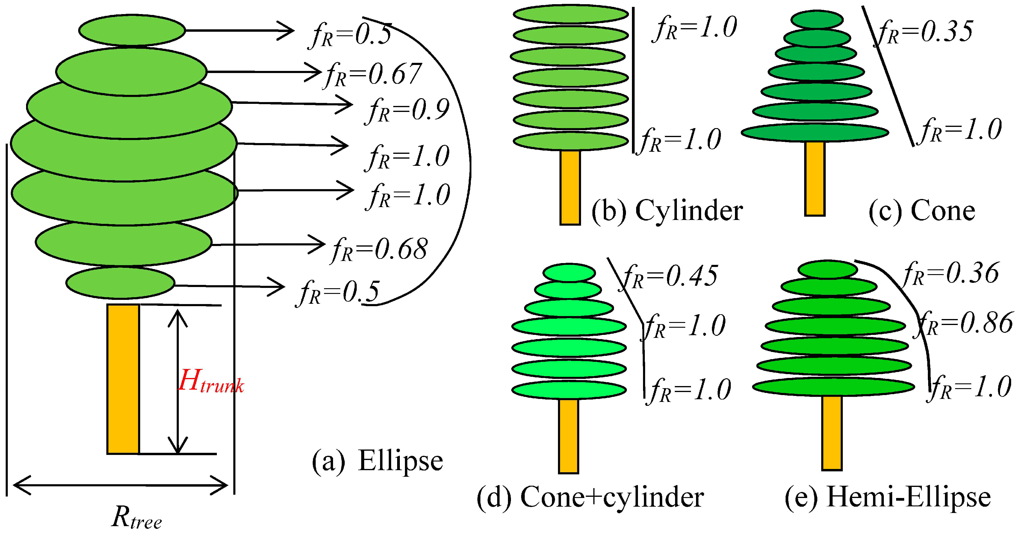
To accurately parameterize each HETOBJ, two new input files, TEXTURE.IN and OBJ_CLUMP.IN, were introduced to define tree locations, radii, and radius adjustment coefficients. The TEXTURE.IN file stores the number of crown HOMOBJs within a HETOBJ, relative coordinates (X_tree, Y_tree) of each HOMOBJ center to the lower-left corner of the HETOBJ, and the maximum radius of each HOMOBJ (R_tree). It is assumed that all HOMOBJs within the HETOBJ have the same circular shape, thickness, LAI, LAD, trunk diameter (D_trunk), and optical parameters. The number of crown HOMOBJs controls the stem density. Changing the (X_tree, Y_tree) of each tree can adjust the spatial distribution of crowns within a HETOBJ. The OBJ_CLUMP.IN file defines the tree radius adjustment coefficients (f_R) that are compared to R_tree for a crown HOMOBJ within a HETOBJ (see Figure 4). Therefore, the R_tree and f_R at different heights can control the tree crown vertical shape to be a sphere, cone, or any other user-defined profiles.

Generally, to model the forests over complex terrains, the digital elevation model (DEM) with triangles should be used. The DEM triangles are first generated as solid soil polygons. To generate trees on DEM, the forest inventory data for all trees in the DEM region should be provided, including their species, heights, positions, crown radii, crown lengths (H_crown), trunk lengths (H_trunk), and LAIs. However, for each soil triangle (may be irregular), the inside trees must be separated from the outside trees. Only the contained trees are used to summarize the important structure parameters for HETOBJ, including the tree number, local positions, tree height ranges, LAI, crown radius ranges, H_crown, and H_trunk. Based on these tree parameters, the soil polygon is simply replicated a few times to generate one trunk and a few crown HETOBJs by shifting the z values from zero to the top tree height contained in the HETOBJ. When z is zero, one trunk HETOBJ is created first with vertical thickness of H_trunk. When z is larger than H_trunk, the z shifting step is estimated as

$$\Delta Z=\frac{f_{shape}{H}_{crown}}{LAI},$$

(3)

where f_shape is 0.24 or 0.12 for ellipsoid or cone shaped crowns according to leaf volume density. Figure 5 shows the generated 3D scenes on a single slope (a–c) and a ridge (d–f). Figure 5a–c are similar to Figure 3a–c, except the slope and tree numbers. Figure 5d–e shows a forest stand with 25 cone-shape trees on a ridge (d), and its abstraction using 78 HETOBJs (e), as well as the dynamically projected object sequence ID image of (e) using the method in Section 3.2. The two large triangles in (Figure 5f) are the two soil polygons to compose the ridge.

3.2. Dynamic Projection of HETOBJ

In RAPID, the leaves in a HOMOBJ are dynamically generated and projected into a 2D pixel array (Figure 6a). First, according to the basal area, LAI and leaf size parameters of a porous object, the number of leaves within the porous object, is estimated. Then, the center points, zenith angles, and azimuth angles for all leaves are randomly generated, where the center points and azimuth angles use a uniform random function; and leaf zenith angles follow the LAD function. Once randomly generated, each leaf has spatially explicit coordinates and is projected into the 2D pixel array. To observe a leaf envelope in the array, the mean leaf pixel size should be at least 9. Otherwise, the leaf will be neglected, and will not be drawn. Then, the 2D array size should be at least 3000 by 3000 for a 100 m by 100 m scene if the leaf length is 10 cm. If the scene is 1 km by 1 km, the array size will be larger than 30,000 by 30,000 (30,000 width × 30,000 height × 4 bytes = 3.6 × 10⁹ bytes = 3.4 GB). Considering that at least two projection arrays (sun and viewer directions) should be used simultaneously, the memory costs of two arrays will be approximately 7 GB. Another important memory cost concerns the view factors, which exponentially increases with the scene size. As a result, the scene has to be limited to a certain size based on the random-access memory (RAM) available. Thus, the subdivision method should be used to run the km-scale scene on the PC. However, subdivision does not significantly reduce computation cost, and introduces additional complexity.

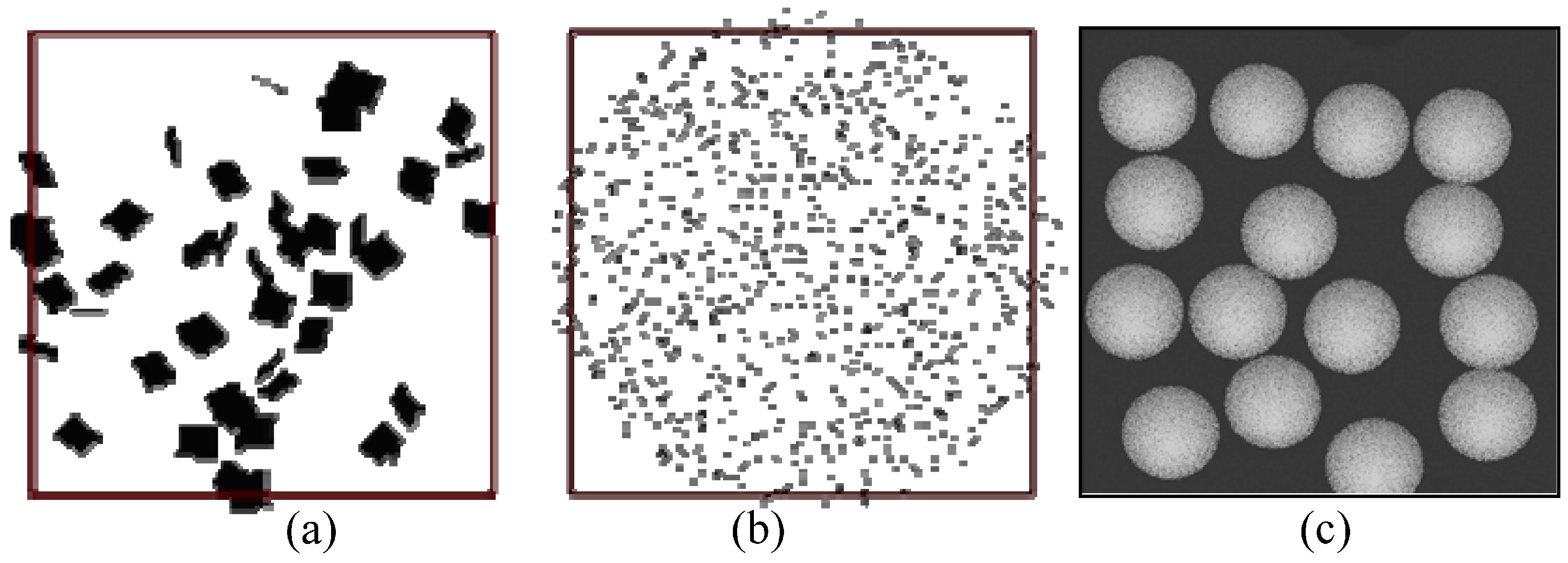
In RAPID3, instead of projecting many finite-size leaves (Figure 6a), points (pixels) are used to render a HOMOBJ or HETOBJ (Figure 6a–c). The point number N is proportional to LA × G(Ω_in), where LA is the total leaf area of a HETOBJ; G is the G-function [41], defined as the averaged projection area of all possible leaf angles along the projection direction Ω_in:

$$G\left({\mathsf{\Omega }}_{in}\right)={\displaystyle \sum _{\phi =0}^{2\pi }{\displaystyle \sum _{\theta =0}^{\pi /2}f\left(\theta \right)}\left|\mathsf{\Omega }\left(\theta ,\phi \right)\cdot {\mathsf{\Omega }}_{in}\right|}\times \sin \left(\theta \right)\times \Delta \theta \times \Delta \phi ,$$

(4)

where Ω(θ, φ) is the leaf orientation direction with zenith angle θ and azimuth angle φ; f(θ) is the LAD function varying with θ, but independent of φ. As a result, the total pixel number in Figure 6a,b should be equal if the same size target 2D arrays are used. In other words, the gap fractions in Figure 6a,b are the same. However, the same 2D array size can be used to project more HOMOBJs in RAPID3 as long as their gap fractions are kept constant. For example, Figure 6c shows the projected random pixels of the scene defined in Figure 3f.

The following paragraphs explain the projection process using a 2D array P(NX, NY) for a 3D scene with a center of (x_center, y_center, z_center) and a radius (R_sphere) of a circumsphere in a direction Ω(θ, φ). The NX and NY are the size of the array P in the x and y directions.

First, the rotation transformation of the Cartesian coordinate system for any point (x₀, y₀, z₀) in the 3D scene must be performed along the direction Ω:

$$\left[\begin{array}{l}{x}_{view}\\ y_{view}\\ z_{view}\end{array}\right]=\left[\begin{array}{lll}-\sin \phi & \cos \phi & 0\\ -\cos \theta \cos \phi & -\cos \theta \sin \phi & \sin \theta \\ \hspace{1em}\sin \theta \cos \phi & \sin \theta \sin \phi & \cos \theta \end{array}\right]\left[\begin{array}{l}{x}_0-x_{center}\\ y_0-y_{center}\\ z_0-y_{center}\end{array}\right]$$

(5)

Second, a scaling transformation is applied to fit the rotated 3D scene to the 2D pixel array:

$$\begin{array}{l}{x}_{pix}=a\times x_{view}+0.5NX\\ y_{pix}=b\times y_{view}+0.5NY\end{array},$$

(6)

where a and b are the scaling coefficients:

$$\begin{array}{l}a=\frac{2R_{sphere}}{NX}\\ b=\frac{2R_{sphere}}{NY}\end{array}$$

(7)

At the pixel position (x_pix, y_pix), the projected polygon code (PID) will be written into the pixel value [P(x_pix, y_pix) = PID]. To address mutual shadowing, a 2D depth array D(NX, NY) is used to record the relative depth value [D(x_pix, y_pix) = z_view] (distance to the sensor). If another polygon pixel has the same pixel position to the current polygon pixel, the depth value comparison will determine whether or not to overwrite the P and D arrays. This is similar to the commonly used z-buffer method in computer graphics [42]. The z-buffer approach is one solution to the visibility problem, which tests the z-depth of each surface to determine the closest (visible) surface to the sensor.

Based on the above method, together with the number of trees N_tree, the list of tree center coordinates (X_tree, Y_tree) and their radii (R_tree × f_R) of a HETOBJ, N points are randomly generated within the range of tree crowns and projected into the array P and D. Four uniform random numbers using PID as the seed are required to generate a point, including the random tree ID (f₁), random radius (f₂), random azimuth (f₃), and random height (f₄). The PID seed initializes a pseudorandom number generator and produces the same series of random numbers for any view angle. The tree ID (TID) is the floor of N_tree × f₁. Finally, the 3D coordinate (x₀, y₀, z₀) of a leaf point will be

$$\begin{array}{l}{x}_0=X_{tree}\left(TID\right)+R_{tree}\left(TID\right)\times f_R\left(TID\right)\times \sqrt{f_2}\times \cos \left(2\pi f_3\right)\\ y_0=Y_{tree}\left(TID\right)+R_{tree}\left(TID\right)\times f_R\left(TID\right)\times \sqrt{f_2}\times \sin \left(2\pi f_3\right)\\ z_0=z\left(x_0,y_0\right)+h\times f_4\end{array},$$

(8)

where z(x, y) is the plane equation of the HETOBJ bottom plane, and h is the thickness of the HETOBJ.

3.3. Estimation of View Factors and Single Scattering

In an arbitrary incident direction Ω, all objects in a 3D scene are sorted by the z-buffer values along the direction. Then, the objects are drawn in sequence using the z-buffer algorithm. For example, if object i is under another object j, i will be first rendered into the projection array P. The total number of i pixels in the direction Ω is N_i(Ω). Then, object j will be projected into the array P. Since j may overlap i, resulting in replacement of i with the j value, the number of i pixels will decrease (noted as T_i(Ω)), and the number of overlapped pixels are recorded as N_ij(Ω). After repeating the projection for all discretized directions of the 2π hemispheric sky (discretization is the same as RAPID), the view factor between i and j will be

$$F_{ij}=\frac{{\displaystyle \sum _{\mathsf{\Omega }}^{2\pi }{N}_{ij}\left(\mathsf{\Omega }\right)}}{{\displaystyle \sum _{\mathsf{\Omega }}^{2\pi }{N}_i\left(\mathsf{\Omega }\right)}}.$$

(9)

Note that each object has two sides: facing (+) or back to (−) the incident direction. Since j⁺ and i⁻ will not see each other, their view factors will be zero. The F_ij is in fact the view factor of j⁻ over i⁺.

Since the porous object i has a visible thickness, and the leaf points within i have a uniform vertical distribution, some projected pixels of i may overlap existing i pixels, resulting in self-overlapping. Compared to HOMOBJ, the HETOBJ contains a few HOMOBJs, which increases the self-overlapping possibility. Thus, the inner multiple scattering of a HETOBJ should be considered. By recording the number of self-overlapped pixels of i as N_ii(Ω), the inner multiple scattering is included by new inner view factors (F_ii).

$$F_{ii}=\frac{2{\displaystyle \sum _{\mathsf{\Omega }}^{2\pi }{N}_{ii}\left(\mathsf{\Omega }\right)}}{{\displaystyle \sum _{\mathsf{\Omega }}^{2\pi }{N}_i\left(\mathsf{\Omega }\right)}}$$

(10)

Assume that the total incident light is defined as 1.0 with a diffuse fraction (k_d). The single scattering of i⁺ and i⁻ from diffuse light will be

$$E_{i^{+},\mathrm{dif}}=\frac{{\rho }_i\times {\displaystyle \sum _{\mathsf{\Omega }}^{2\pi }{T}_{i^{+}}\left(\mathsf{\Omega }\right)+{\tau }_i\times {\displaystyle \sum _{\mathsf{\Omega }}^{2\pi }{T}_{i^{-}}\left(\mathsf{\Omega }\right)}}}{{\displaystyle \sum _{\mathsf{\Omega }}^{2\pi }{N}_i\left(\mathsf{\Omega }\right)}}\times k_d,$$

(11)

$$E_{i^{-},\mathrm{dif}}=\frac{{\rho }_i\times {\displaystyle \sum _{\mathsf{\Omega }}^{2\pi }{T}_{i^{-}}\left(\mathsf{\Omega }\right)+{\tau }_i\times {\displaystyle \sum _{\mathsf{\Omega }}^{2\pi }{T}_{i^{+}}\left(\mathsf{\Omega }\right)}}}{{\displaystyle \sum _{\mathsf{\Omega }}^{2\pi }{N}_i\left(\mathsf{\Omega }\right)}}\times k_d,$$

(12)

where ρ_i and τ_i are the equivalent reflectance and transmittance of the object i defined in RAPID. The sunlit fraction of i in the solar incident direction Ω_sun is

$$f_{i,lit}=\frac{T_i\left({\mathsf{\Omega }}_{\mathrm{sun}}\right)}{N_i\left({\mathsf{\Omega }}_{\mathrm{sun}}\right)}.$$

(13)

Then, the direct single scatterings of i⁺ and i⁻ in the solar incident direction Ω_sun are estimated as follows:

$$E_{i^{+},\mathrm{sun}}={\rho }_i\times f_{i,lit}\times f_{LAD,i^{+}}\times \frac{\left(1-k_d\right)}{\cos {\theta }_{sun}},$$

(14)

$$E_{i^{-},\mathrm{sun}}={\tau }_i\times f_{i,lit}\times f_{LAD,i^{-}}\times \frac{\left(1-k_d\right)}{\cos {\theta }_{sun}},$$

(15)

where θ_sun is the zenith angle of the solar direction; the two f_LAD are the upside (+) and downside (−) coefficients to correct the LAD effect (f(θ)) of the horizontal HETOBJs are

$$f_{LAD,i^{+}}={\displaystyle \sum _{\phi =0}^{2\pi }{\displaystyle \sum _{\theta =0}^{\pi /2}f\left(\theta \right)}\left|\mathsf{\Omega }\left(\theta ,\phi \right)\cdot {\mathsf{\Omega }}_{sun}\right|}\times \frac{1+\cos \left(\theta \right)}{2}\times \Delta \theta \times \Delta \phi ,$$

(16)

$$f_{LAD,i^{-}}={\displaystyle \sum _{\phi =0}^{2\pi }{\displaystyle \sum _{\theta =0}^{\pi /2}f\left(\theta \right)}\left|\mathsf{\Omega }\left(\theta ,\phi \right)\cdot {\mathsf{\Omega }}_{sun}\right|}\times \frac{1-\cos \left(\theta \right)}{2}\times \Delta \theta \times \Delta \phi ,$$

(17)

where θ and φ are the zenith and azimuth angle, respectively; the dot products between leaf normal Ω(θ, φ) and sun direction Ω_sun estimate the correction coefficient of sunlit irradiance; (1 + cos(θ))/2 and (1 − cos(θ))/2 represent the upward and downward view fractions for the leaf normal Ω(θ, φ). Combining the diffuse and direct light, the total single scattering of i (+ or −) is expressed as

$$E_i=E_{i,\mathrm{sun}}+E_{i,dif}.$$

(18)

For an inclined HETOBJ, its upper hemisphere differs from that of a horizontal HETOBJ. Thus, the two f_LAD are dependent not only on the LAD, but also on the normal of the HETOBJ (Ω_i):

$$f_{LAD,i^{+}}={\displaystyle \sum _{\phi =0}^{2\pi }{\displaystyle \sum _{\theta =0}^{\pi /2}f\left(\theta \right)}\left|\mathsf{\Omega }\left(\theta ,\phi \right)\cdot {\mathsf{\Omega }}_s\right|}\times \frac{1+\left|\mathsf{\Omega }\left(\theta ,\phi \right)\cdot {\mathsf{\Omega }}_i\right|}{2}\times \Delta \theta \times \Delta \phi$$

(19)

$$f_{LAD,i^{-}}={\displaystyle \sum _{\phi =0}^{2\pi }{\displaystyle \sum _{\theta =0}^{\pi /2}f\left(\theta \right)}\left|\mathsf{\Omega }\left(\theta ,\phi \right)\cdot {\mathsf{\Omega }}_s\right|}\times \frac{1-\left|\mathsf{\Omega }\left(\theta ,\phi \right)\cdot {\mathsf{\Omega }}_i\right|}{2}\times \Delta \theta \times \Delta \phi$$

(20)

Based on the input leaf reflectance and transmittance (ρ_sub-object and τ_sub-object), the equivalent values (ρ_i and τ_i) of the inclined HETOBJ are modified as

$${\rho }_i={\rho }_{sub-object}{\displaystyle \sum _{\phi =0}^{2\pi }{\displaystyle \sum _{\theta =0}^{\pi /2}f\left(\theta \right)}}\times \frac{1+\left|\mathsf{\Omega }\left(\theta ,\phi \right)\cdot {\mathsf{\Omega }}_i\right|}{2}\times \Delta \theta \times \Delta \phi +{\tau }_{sub-object}{\displaystyle \sum _{\phi =0}^{2\pi }{\displaystyle \sum _{\theta =0}^{\pi /2}f\left(\theta \right)}}\times \frac{1-\left|\mathsf{\Omega }\left(\theta ,\phi \right)\cdot {\mathsf{\Omega }}_i\right|}{2}\times \Delta \theta \times \Delta \phi ,$$

(21)

$${\tau }_i={\rho }_{sub-object}{\displaystyle \sum _{\phi =0}^{2\pi }{\displaystyle \sum _{\theta =0}^{\pi /2}f\left(\theta \right)}}\times \frac{1-\left|\mathsf{\Omega }\left(\theta ,\phi \right)\cdot {\mathsf{\Omega }}_i\right|}{2}\times \Delta \theta \times \Delta \phi +{\tau }_{sub-object}{\displaystyle \sum _{\phi =0}^{2\pi }{\displaystyle \sum _{\theta =0}^{\pi /2}f\left(\theta \right)}}\times \frac{1+\left|\mathsf{\Omega }\left(\theta ,\phi \right)\cdot {\mathsf{\Omega }}_i\right|}{2}\times \Delta \theta \times \Delta \phi ,$$

(22)

3.4. Solution of Multiple Scattering

Using the single scattering values and view factors (see Section 3.3) as inputs, Equation (1) is used to solve the average radiosity of each object (B_i) through the Gauss–Seidel iteration method, which was well described in RAPID. Note that the inner view factor (F_ii) has been included, although without explicit indication. After iteration, the final radiosity is

$$B_i=E_{i,sun}+E_{i,dif}+{\chi }_i{\displaystyle \sum F_{ij}{B}_j}i,j=1,2,\dots 2N.$$

(23)

It is obvious that HETOBJ is a non-Lambertian object. The anisotropy of reflectance is assumed to be mainly determined by the directionality of single scattering caused by the significant radiance difference between sunlit and shaded leaves or branches. Since the sunlit fractions of all objects are already known from dynamic projections, the sunlit and shaded radiosity of i are estimated as follows:

$$\begin{array}{l}{B}_{i,dif}=E_{i,dif}+{\chi }_i{\displaystyle \sum F_{ij}{B}_j}\\ B_{i,sun}=\frac{E_{i,sun}}{f_{i,lit}}+B_{i,dif}\end{array}$$

(24)

In fact, the sunlit and shaded radiosity for each HETOBJ should also be angularly dependent. The isotropic average assumption in Equation (24) may cause potential errors on the BRF.

3.5. Solution of BRF of a 3D Scene

Since the total incidence is 1.0, the BRFs of a 3D scene are weighted averages of radiosity from all objects in each view direction v (Equation (25)).

$$BRF(v)=\frac{{\displaystyle \sum _{i=1}^N\left[B_{i,lit}{A}_{i,lit}(v)+B_{i,dif}{A}_{i,dif}(v)\right]}}{{\displaystyle \sum _{i=1}^N\left[A_{i,lit}(v)+A_{i,dif}(v)\right]}},$$

(25)

where N is the number of all objects, including both solid facets and HETOBJs; $A_{i,lit}$ or $A_{i,dif}$ is the viewed area of a sunlit or shaded object i that is visible to the viewer.

The weights are the fractions of viewed object areas (A_i,lit and A_i,shd) with respect to the sum of the viewed areas of all objects (the denominator in Equation (25)). In traditional radiosity models, automatic subdivision of planar facets into smaller subfacets is used to make each subfacet either sunlit or shaded. Similarly, porous objects are divided into two parts: the sunlit and shaded part. Without separating the sunlit from the shaded part, the BRF contrast (e.g., between forward and backward view directions) and hotspot effect decrease significantly. That is why the radiosity has been decomposed into sunlit and shaded parts (Equation (24)). Thus, determining whether a pixel is sunlit is the key problem for BRF synthesis.

In RAPID, affine transform equations were used to determine if a pixel with an object ID i in the view pixel array is visible in the sun projection array or not. If visible, the pixel is sunlit; otherwise, shaded. In this way, the $A_{i,lit}$ or $A_{i,dif}$ is accurately estimated. However, by using randomly scattered pixels (Figure 6b–c) instead of collections of subleaf pixels (Figure 6a), the error from an affine transform for a HETOBJ increases, resulting in overestimating shaded fractions at the large view zenith angle (VZA). Only in the hot spot direction, the error is zero. In addition, affine transform equations should be built for each subleaf; thus, the computation costs with an affine transform solution and the RAM costs for coefficients storage are unacceptable for large scenes.

In RAPID3, to reduce the error, the computation and the RAM costs from the affine transform, Equation (26) is developed to directly transform the pixel coordinates (x_pix, y_pix) from the viewer direction to the sun direction (x_{pix_sun}, y_{pix_sun}). The idea is to combine the z-buffer values (z_view) and pixel positions (x_pix, y_pix) in viewer projection arrays P_view to inverse 3D coordinates of leaf points, and then project them back into the solar projection array P_sun at location (x_{pix_sun}, y_{pix_sun}). If the polygon ID of P_view (x_pix, y_pix) matches P_sun (x_{pix_sun}, y_{pix_sun}), this pixel is sunlit; otherwise, shaded. However, due to the round-off errors from floating point values to integer values, the pixel positions may be shifted one to two-pixel widths, thus leading to underestimated sunlit fractions.

$$\begin{array}{l}\left[\begin{array}{c}{x}_{pix\_sun}\\ y_{pix\_sun}\\ z_{pix\_sun}\end{array}\right]=\left[\begin{array}{ccc}a& 0& 0\\ 0& b& 0\\ 0& 0& 1\end{array}\right]\times \left[\begin{array}{lll}-\sin {\phi }_{sun}& \hspace{1em}\cos {\phi }_{sun}& 0\\ -\cos {\theta }_{sun}\cos {\phi }_{sun}& -\cos {\theta }_{sun}\sin {\phi }_{sun}& \sin {\theta }_{sun}\\ \hspace{1em}\sin {\theta }_{sun}\cos {\phi }_{sun}& \sin {\theta }_{sun}\sin {\phi }_{sun}& \cos {\theta }_{sun}\end{array}\right]\\ \hspace{1em}\hspace{1em}\hspace{1em}\times \left[\begin{array}{ccc}-\sin \phi & -\cos \theta \cos \phi & \sin \theta \cos \phi \\ \cos \phi & -\cos \theta \sin \phi & \sin \theta \sin \phi \\ 0& \sin \theta & \cos \theta \end{array}\right]\times \left[\begin{array}{l}(x_{pix}-0.5NX)/a\hfill \\ (y_{pix}-0.5NY)/b\hfill \\ z_{view}\hfill \end{array}\right]+\left[\begin{array}{l}0.5NX\hfill \\ 0.5NY\hfill \\ 0\hfill \end{array}\right]\end{array}$$

(26)

Unlike planar facets, leaf points do not have an explicit normal vector (similar to the voxel concept in 3DRT), whose scattering is isotropic. In RT theory, a scattering phase function is required to describe the anisotropy. In this paper, RAPID was used to presimulate the sunlit fractions (f_i,∆lit) of a virtual HOMOBJ using the LAI, LAD, and thickness values of a HETOBJ i to represent the scattering anisotropy of this HETOBJ in all directions. These sunlit fractions are used to correct the $A_{i,lit}$ or $A_{i,dif}$ in Equation (25):

$$\begin{array}{l}{\widehat{A}}_{i,lit}\left(\nu \right)=A_{i,lit}\left(\nu \right)\times f_{i,\Delta lit}\left(\nu \right)\\ {\widehat{A}}_{i,dif}\left(\nu \right)=A_{i,lit}\left(\nu \right)\times \left(1-f_{i,\Delta lit}\left(\nu \right)\right)+A_{i,dif}\left(\nu \right)\end{array}$$

(27)

4. Model Evaluations

4.1. RAMI-3 Scenes and Main Inputs

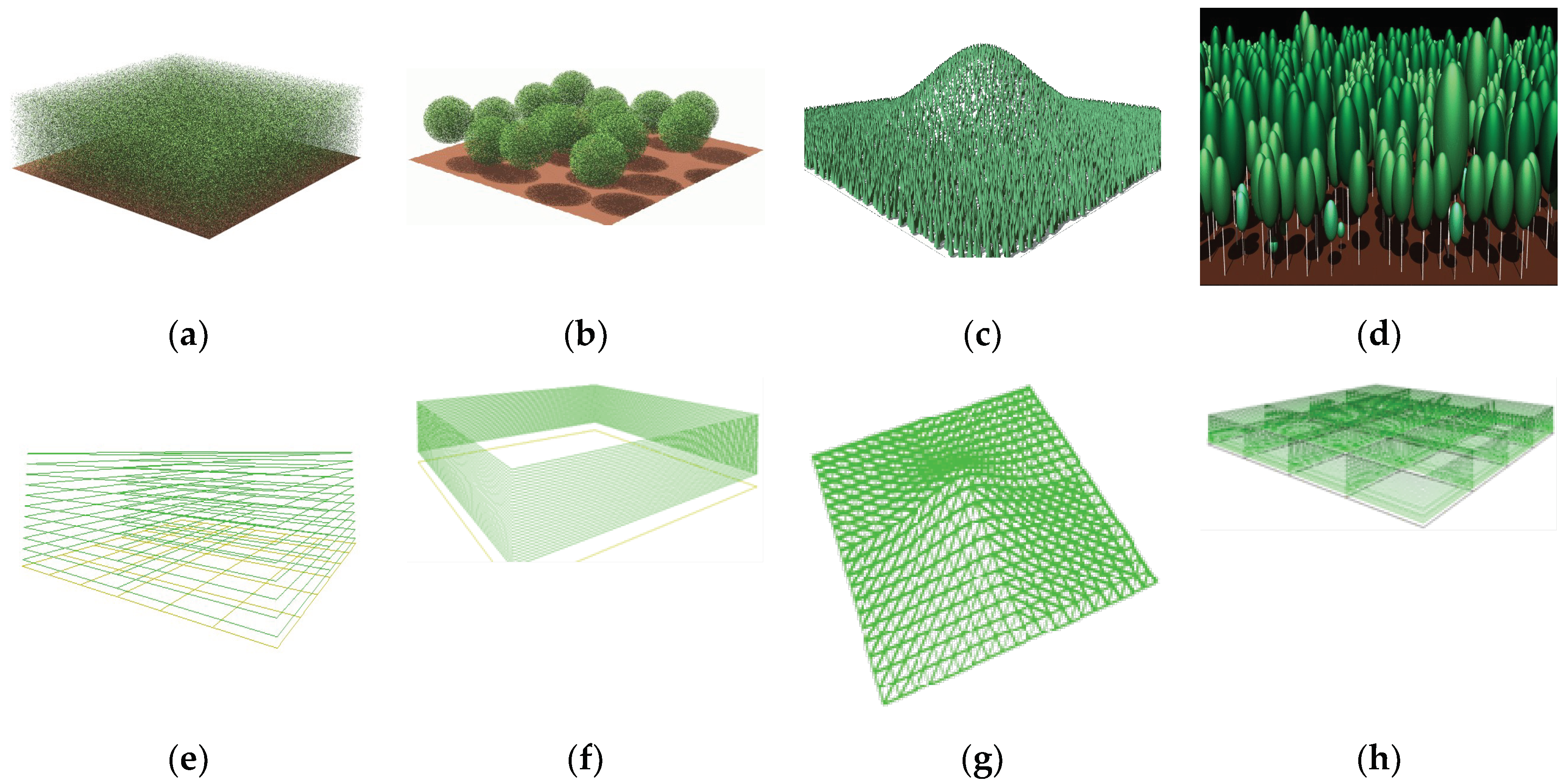
Five RAMI-3 cases (Figure 7), including the homogeneous canopies (HOM03 and HOM13), the discrete forest (HET01), the pine forest with topography (HET03), and the birch forest with a complex vertical structure (HET05), have been chosen to test the BRF produced by RAPID3. The main input parameters are shown in

Table 1. Main inputs for five RAMI-3 test cases.

	HOM03	HOM13	HET01	HET03	HET05
LAI of scene (m2m−2)	3.0	3.0	2.35	2.0358	0.388
Fraction cover	1.0	1.0	0.471	0.4072	0.289
Stems	--	--	15	10,000	1800
Maximum slope [deg]	0	0	0	68	0
True leaf count	238,732	59,683	2.4 million	64.8 million	0.5 million
HETOBJ count	79	79	27	31,200	320
SZA [deg]	20 or 50	20 or 50	20 or 50	40	20 or 50
Soil reflectance [red/NIR]	0.127/0.159	0.127/0.159	0.127/0.159	0.86/0.64	0.127/0.159
Leaf reflectance [red/NIR]	0.0546/0.4957	0.0546/0.4957	0.0546/0.4957	0.08/0.45	0.08/0.47
Leaf transmittance [red/NIR]	0.0149/0.4409	0.0149/0.4409	0.0149/0.4409	0.03/0.30	0.04/0.48
Trunk reflectance [red/NIR]	--	--	--	0.14/0.24	0.30/0.38

, including structural parameters, solar zenith angle (SZA), and the optical reflectance or transmittance in red and near infrared (NIR) bands. Compared to the scenes using “true” leaf triangles, the HETOBJ scenes have a significantly reduced number of polygons (e.g., only 0.2% in HET03). Even when compared to RAPID scenes using HOMOBJs, the number of polygons of HETOBJ scenes are significantly reduced (only 6–8%).

4.2. Model Comparisons

To evaluate the RAPID3 performance, the RAMI online model checker (ROMC, http://romc.jrc.ec.europa.eu) was used, which is a web-based tool allowing model developers to check their canopy RT model performance using assembled reference data (ROMCREF) [43]. ROMC has two modes: the debug and validate mode. Since the debug mode is better to guide model improvement, the debug mode was used in this study. The BRF in the solar principal plane (brfpp) is selected for comparisons. Generally, ROMCREF has three gray-colored envelopes (similar to error bars) corresponding to 1, 2.5, and 5% variations from the “surrogate truth” BRF. The root mean squared error (RMSE) provided by the ROMC is used to assess the accuracy.

4.2.1. HOM03 and HOM13

HOM03 and HOM13 refer to the same vegetation canopy but with different LAD and leaf size.

HOM13 has a planophile LAD (PLA) and a leaf radius of 0.1 m, while HOM03 has an erectophile LAD (ERE) and a leaf radius of 0.05 m.

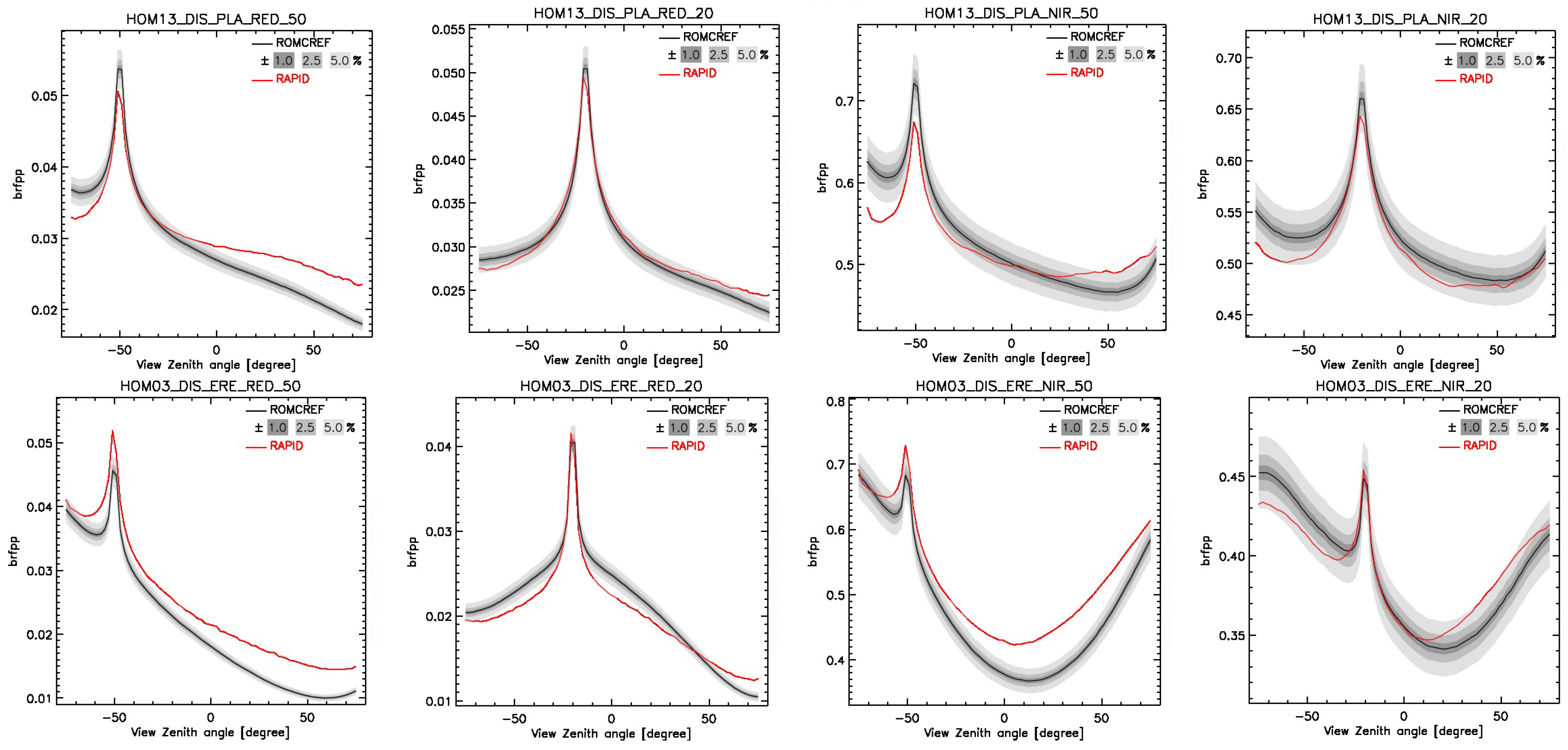
Figure 8 shows eight groups of BRF results from both HOM13 and HOM03. In the subtitles, “HOM13_DIS_PLA” and “HOM03_DIS_ERE” refer to HOM13 and HOM03, respectively; the RED and NIR mean the red and NIR band; the 20 and 50 refer to SZA. The RAPID BRF curves are generally consistent in shape with the reference data provided by ROMC (ROMCREF in Figure 8) except a few biases (mean RMSE = 0.014, see

Table 2. Bidirectional reflectance factor (BRF) RMSE at the red and NIR band, two SZA (20° and 50°) on HOM13 and HOM03.

RMSE	RED, 20	NIR, 20	RED, 50	NIR, 50	Mean
HOM13 (PLA)	0.0009	0.0124	0.0032	0.0267	0.0108
HOM03 (ERE)	0.0016	0.0146	0.0038	0.0486	0.0172
Mean	0.0013	0.0135	0.0035	0.0377	0.0140

). The RMSE at SZA 20° is lower than that at SZA 50°, especially in the NIR band (0.0146 vs 0.0486). There are two types of errors at SZA 50°: (a) lower BRF contrast between backward and forward direction; and (b) overestimation for ERE canopy. The accuracy of the PLA canopy is higher than that of the ERE canopy (0.0108 vs 0.0172).

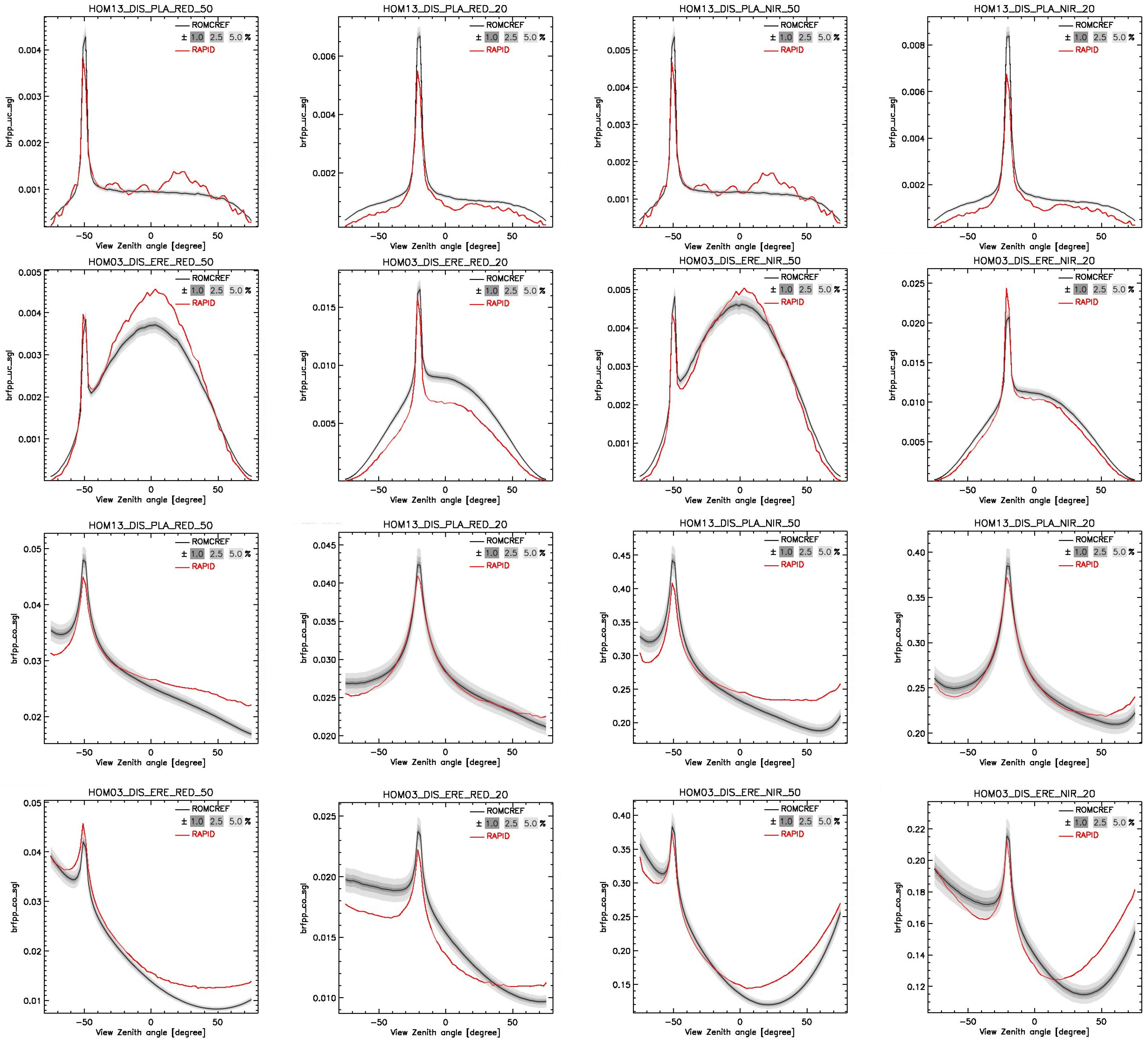
To further determine the error sources, the single scattering results from soil (brfpp_uc_sgl) and leaf (brfpp_co_sgl) components are shown in Figure 9. Despite some small variations, the simulated soil single scattering BRF curves match well with ROMCREF. The largest errors (0.002) for soil occurred in the HOM03 canopy at the red band and SZA of 20°, which is too small to affect the whole BRF. Therefore, the major error source should be from leaf components, which are confirmed in the HOM03 ERE canopy (the last row in Figure 9). The maximum RSMEs of brfpp_co_sgl appear at SZA 50°, which are 0.0239 for NIR and 0.0028 for the red band.

The reason for the higher errors on leaf components is mainly due to the use of single sunlit radiance of porous objects for all view directions. In fact, when viewing a porous object from different view angles, an observer would see different leaves, which would lead to different view fractions of sunlit and shaded leaves. This view fraction effect has been corrected by RAPID. In addition to that effect, the mean sunlit radiance for the object, assumed constant in RAPID, may also vary with the view angle. Especially for vertical leaves, an observer will see the more positive side (facing the sun) of sunlit leaves in the backward directions than in the forward directions, while the more negative side of sunlit leaves in backward directions will be seen than that in the forward directions. The positive and negative sides of leaves may have significantly different radiances. Without considering the directional variation of sunlit leaf radiance, the simulated RAPID BRF values exhibit a high possibility of having lower contrast in the backward and forward directions.

As a result, RAPID3 does not have perfect simulation accuracy on homogeneous canopies with vertical LAD. However, similar to the previous study on improving the performance of the scattering by arbitrarily inclined leaves (SAIL) model [44], the constant assumption of mean sunlit radiance for porous objects can be removed in a future study. Additionally, RAPID3 has more advantages for heterogeneous (HET) canopies than HOM canopies. In the following sections, three HET canopies are further used to test RAPID3.

4.2.2. HET01

The HET01 scene was created by only 27 HETOBJs and one soil polygon, which is approximately 0.01% of the “true” polygon number described in RAMI-3. All the tree locations are specified using the values on the RAMI website. However, the tree height is assumed the same (25 m) for simplicity. The tree radius ratio (f_R) defined in OBJ_CLUMP.IN is from zero (top crown) to 1.0 (the height with maximum radius), then to zero (bottom crown) to maintain the ellipsoid crown.

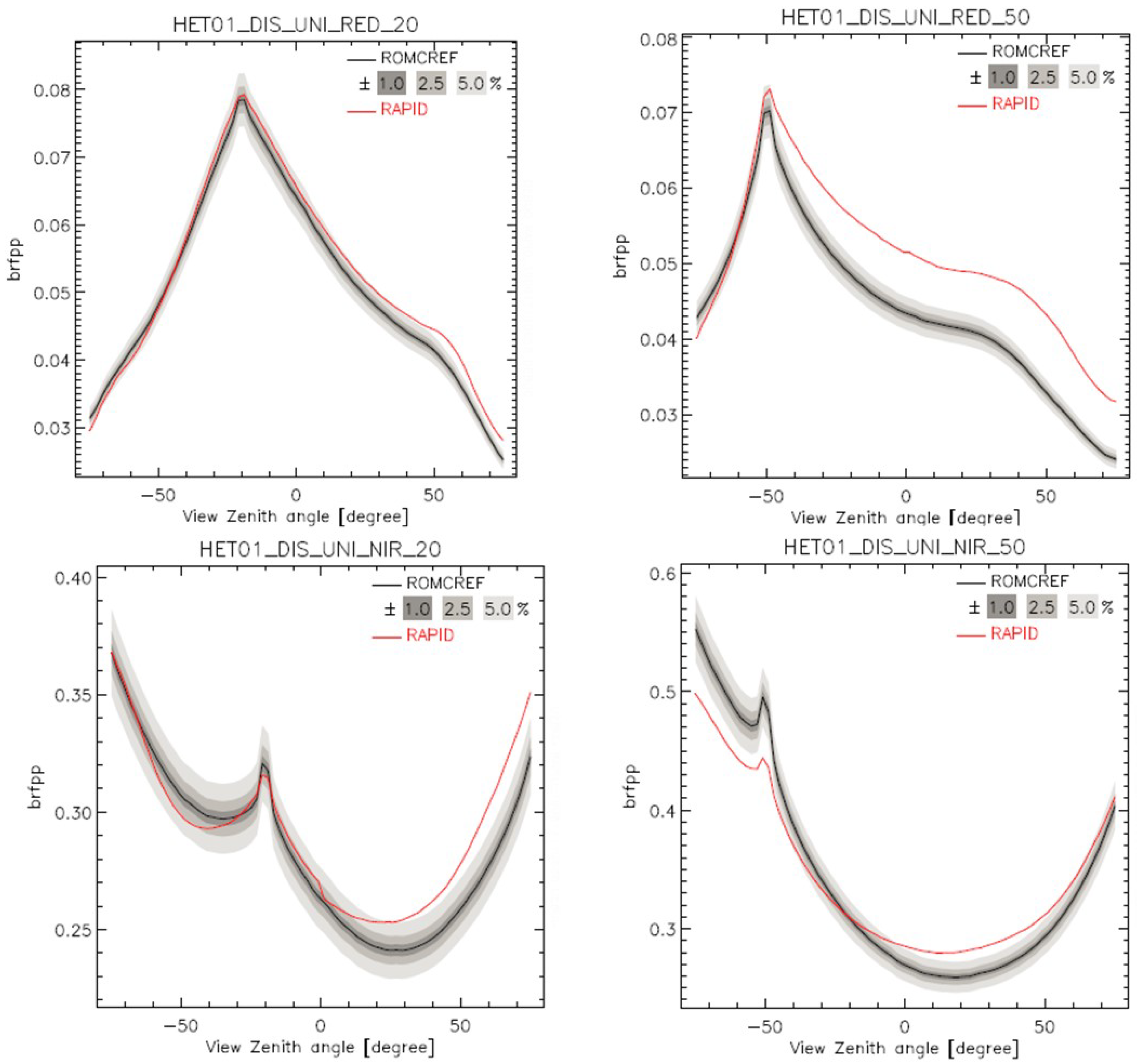
Figure 10 shows the BRF results of HET01. When SZA is 20°, the simulated BRF values and shape match well with ROMCREF data except for small errors in NIR, including the underestimation (at approximately −0.01) in backward directions, and an overestimation in forward directions (<0.025). However, for SZA 50°, the relative error increases in the forward direction for red band (at approximately +25%) and the backward direction for the NIR band (−9%). This kind of error is due to the assumption of constant sunlit radiance for all view directions, which has been explained in Section 4.2.1. Since the vegetation fraction cover of HET01 is only 0.471, the error from the leaf component will affect the BRF values less than those in the HOM canopies with 100% coverage. Therefore, the four simulated cases are still acceptable (RMSE = 0.0143), and the trend is consistent.

4.2.3. HET03

The HET03 case evaluates the BRF simulations for spatially heterogeneous coniferous forests containing some degree of soil topography (Gaussian shaped surface). This case is closest to our research objective. There are a total of 10,000 nonoverlapping trees randomly distributed over the Gaussian surface. The finite sized foliage is a disc with a radius of 5 cm. Since the LAI of a single tree is 5.0, there will be 64.8 million discs, which is excessive for achieving a fast calculation.

There are 31,200 HETOBJs and 800 soil triangles used to create the 500 m by 500 m 3D scene. Each HETOBJ has a vertical projection area of 312.5 m² containing approximately 13 trees. The tree locations are the exact ones from the RAMI website. The tree radius ratio (f_R) is linear from zero (top crown) to 1.0 (bottom crown) to form a cone shaped tree crown.

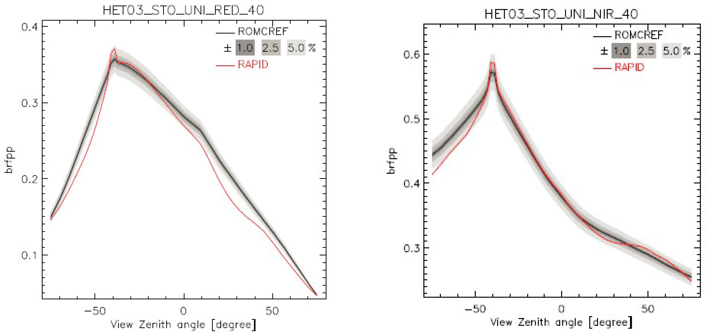
Since the RAMI ROMC only provides one SZA case (40°), Figure 11 shows the comparison results with a SZA of 40°. The error is comparable to HET01 and HOM scenes with RMSE of 0.0137 for the red band and 0.0214 for the NIR band. As the soil reflectance is very high (similar to a snow background), and its view fraction varies from 0.65 (nadir) to 0.16 (off-nadir 75 deg), the BRF is largely affected by soil view fractions and radiances. Furthermore, in the red band, the leaf radiance is significantly lower than that of the soil (approximately 5% and 40% for the sunlit and shaded part, respectively). The contribution of the soil radiance to the total BRF is very large in both the red (58% to 94%) and NIR band (9% to 58%). Thus, the error is mainly from the view fractions of the soil background (Section 3.5). In the NIR band, the leaf radiance is larger and becoming comparable to that of the soil (approximately 60% and 230% of the sunlit and shaded soil radiance, respectively). The slight drop of the simulated BRF in the backward direction refers to the underestimation of the sunlit crown fractions.

4.2.4. HET05

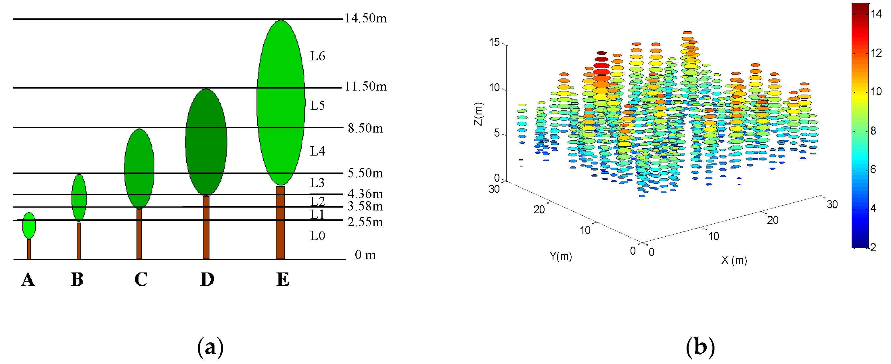
The HET05 case evaluates the BRF simulations for a vertically complex forest containing five classes of trees (A to E in Figure 12a). These birch trees have five heights varying from 2.5 m to 14.5 m. The scene LAI is low (0.388), but the tree density is high (1800 plants/ha). Each class of tree has its own leaf and trunk reflectance and transmittance. Therefore, this scene is the most complicated one to parameterize RAPID3.

There are 320 HETOBJs and 16 soil polygons used to create the 120 m by 120 m 3D scene (Figure 7h). Each HETOBJ or soil polygon has a size of 30 m by 30 m. The number of crowns within the HETOBJ varies with height. For simplicity, the vertical profile is divided into seven regions (L0 to L6 in Figure 12a). In L0, there is only one class A. In L6, there is only one class E. From L1 to L5, there are 2~4 tree classes, which means that these classes must be averaged to assign a mean LAI and mean reflectance and transmittance for the HETOBJ. The averaging process used the crown leaf areas as weights. Finally, the scene was divided into 20 layers within seven regions. Since the tree radius in these layers is not constant, it should be calculated for each crown in each HETOBJ and listed in the file TEXTURE.IN. Figure 12b shows the crown HOMOBJs (circles) contained in the 20 HETOBJs, where the color represents the height.

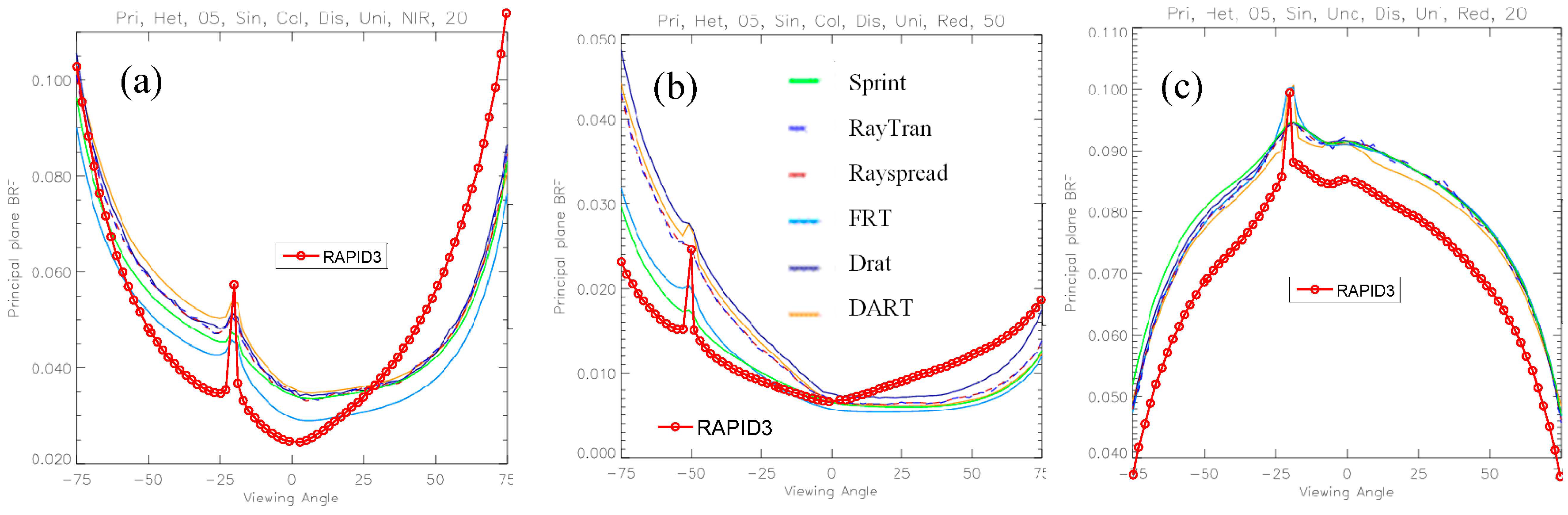
Figure 13 shows the BRF comparison results with SZA of 20° and 50°. The mean RMSE is 0.0133, which is also comparable to previous cases. The best simulation (RMSE = 0.0037) is in the red band at SZA of 20°. At SZA of 50°, there is a drop in the red band in the backward directions, causing a higher RMSE (0.0068). The sunlit fraction in the hotspot direction is correctly simulated as 100%. The BRFs in the hotspot direction also match well with ROMCREF data. These observations mean that the multiple scattering solutions (Section 3.4) and sunlit radiances of HETOBJs should have good accuracy. The major errors in the other directions should not be from radiance estimation but from the sunlit fraction estimation method.

Figure 14 shows the singly scattered BRF of a leaf (a and b) and soil (c). The hotspot BRFs are comparable to other models. However, in the red band for a leaf (Figure 14b), there are significant underestimations in backward directions and overestimations in forward directions. This phenomenon can also be found in previous cases, which is mainly due to the constant sunlit radiance assumption and the effect of round-off errors explained in Section 3.5. In the red band for the soil (Figure 14c), except in the hotspot direction, the BRFs are all underestimated, which is due to the extremely low tree LAI (<0.4), causing many scattered soil pixels within the crown shadow envelope. Theoretically, most soil pixels should be determined as sunlit. However, the neighbors may be crown pixels. One pixel shifting error due to round-off may fail to find the sunlit soil pixel, resulting in a lower sunlit soil fraction, causing the lower soil single scattering in Figure 14c.

Both the single scattering (Figure 14) and total scattering (Figure 13) show that there are two major error sources: the sunlit fraction error caused by the round-off problem, and the constant sunlit radiance assumption. The round-off problem can be partially corrected by increasing the pixel array size or adopting some refining processes. A possible refining method would be to borrow the anti-aliasing technique used in computer graphics [45]. The constant sunlit radiance assumption will be removed in future versions of RAPID3.

4.3. Computation Time Cost Analysis

Table 3. Computation time costs of RAPID3 using RAMI-3 test cases.

Time Cost (Seconds)	HOM03	HOM13	HET01	HET03	HET05
View factor stage	12	12	80	186	34
BRF stage	11	11	90	511	7
Multiple scattering	2	2	56	60	4
total	25	25	226	757	55

shows the computation time of the five test cases using a PC with central processing unit (CPU) at 2.5 GHz, with 4 GB RAM on 64-bit Windows 7 OS. The maximum time cost is approximately 13 min for the HET03 scene (500 m by 500 m). If RAPID had been used to run HET03, it would have used 25 times the polygon number. As a result, the computation time could be 25log(25) times of that using RAPID3. By using the subdivision method with multiple PCs, the computation time could be reduced to the same level; however, it is not convenient for users. Except for HET03, the 3D scene used flat ground, which means the infinite replication method can be used. Thus, RAPID can simulate BRF with a comparable computation time to RAPID3 for HOM03, HOM13, HET01, and HET05. By contrast, the advantage of RAPID3 is in simulating a complex landscape scene with topography, such as HET03.

The HET03 scene was then tested on a faster computer (a CPU at 3.2 GHz, with 4 cores and 8 GB RAM on 64-bit Windows 7 OS). The resultant time cost was not significantly reduced (606 s) because the multiple cores were not exploited in this study. Generally, the computation time cost of a model is mainly affected by three factors: scene size, algorithm complexity, and CPU or graphics processing unit (GPU) resources. This paper only focused on the reduction of scene size with the corresponding RT solution method. In the future, RAPID3 will be further accelerated by exploring the capacity of multiple CPU cores or GPU resources.

4.4. Topography Effect Analysis

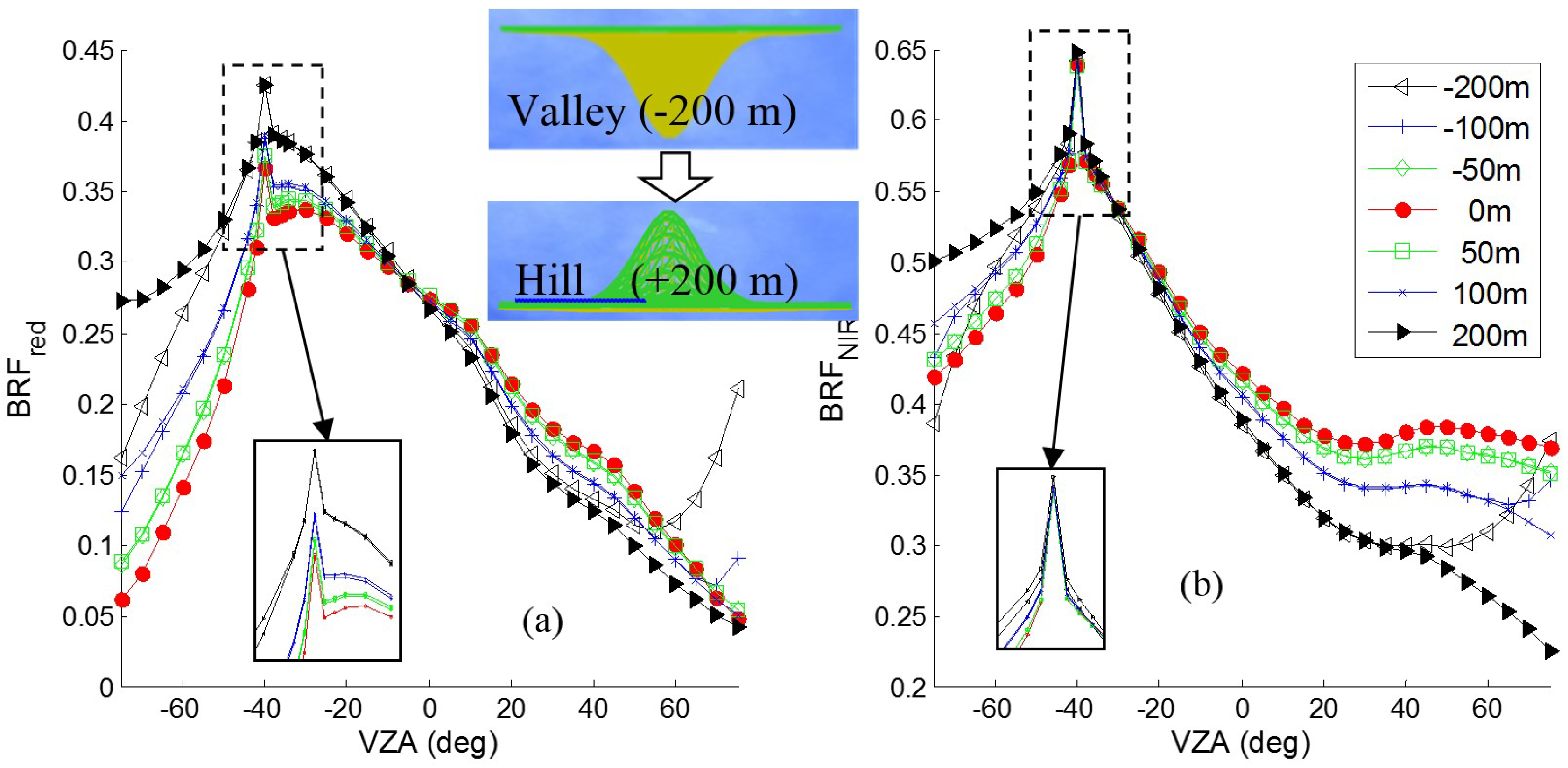
By scaling the z values of HET03 with a coefficient from −2.0 to 2.0, the topographic effect on BRF (from deep valley, flat ground to steep hill) was simulated. Figure 15 shows the BRF curves varying with the z(0, 0) at the scene center (named ZC), representing the steepness and topography type. Major findings include:

• The backward BRFs of nonflat ground (ZC ≠ 0) are generally larger than those over flat ground (ZC = 0) and increase with $\left|ZC\right|$. In forward directions, the BRFs of nonflat ground (ZC ≠ 0) are generally smaller than those over flat ground (ZC = 0), and decrease with $\left|ZC\right|$.
• It is interesting that the BRFs over the valley and hill are almost the same if their $\left|ZC\right|$ are equal (e.g., ZC = ±50 m or ±100 m). However, for ZC = ±200 m, the BRF difference increases (0.02~0.15) when VZA > 50°.
• At the nadir direction, the BRF varies less with ZC in the red band (up to 0.01) but more in the NIR band (up to 0.06, see Figure 15b).
• At the hotspot direction, the BRF varies less in the NIR band (<0.01) but more in the red band (up to 0.06, see Figure 15a).
• The maximum BRF variation occurs in backward directions at the red band and in forward directions at the NIR band.

This topography simulation is the first case study on simulating BRF over both valleys and hills. It demonstrates the suitability of the RAPID model to understand how the topography affects the BRF.

5. Conclusions

By extending the porous object concept in the RAPID model from homogeneous to heterogeneous conditions, the RAPID3 model has been proposed specifically for km-scale RT simulation. It is the first 3D model focusing on a fast RT solution of vegetation canopies in mountainous areas. The major advance in the development of RAPID is the significantly lower computation time of BRF at the km-scale (approximately 13 min). The heterogeneous porous object (HETOBJ) concept is the key innovation that reduces the complexity of 3D forest scenes significantly. The corresponding radiosity method has been adapted from HOMOBJ to HETOBJ. Five RAMI-3 scenes, from homogenous canopies (HOM03/13) to discrete forest canopies (HET01, HET03, and HET05), have been used to evaluate RAPID3. Based on HET03, RAPID3 also simulated the enhanced contrast of BRF between the backward and forward directions due to topography based on the HET03 scene. This analysis demonstrated the suitability of the RAPID model to understand how the topography affects the BRF.

The major improvements on the RAPID model are as follows:

• Better visibility determination: The painter algorithm has been updated as the z-buffer algorithm, which is more accurate regarding the visibility determination between large objects.
• New inner view factors: The inner multiple scattering of a HETOBJ are considered using the new inner view factors (F_ii), which compensated for the underestimation of multiple scattering.
• Less memory costs: Random points (pixels) instead of many finite-size leaves are projected to render a HOMOBJ or HETOBJ, which reduced the memory requirement of large pixel array size for the km-scale in RAPID. Due to the z-buffer values, the affine transform used in RAPID has been replaced by a simple matrix transform equation to decide whether a pixel is sunlit or not, which reduced the memory costs related to storing the affine transform coefficients of all subleaves.

There are also two main limitations to the current version of RAPID3:

1.

Large errors in some cases (e.g., HET05): The mean RMSE of the simulated BRF is 0.015; however, the maximum BRF bias from ROMCREF can be up to 0.02 and 0.05 in the red and NIR band, respectively. These errors mainly originate from the sunlit fraction estimation error and the isotropic sunlit radiance assumption on HETOBJ.

2.

Considerable effort to generate RAPID3 scenes: The RAPID GUI has not been extended to automatically transform RAPID scenes to RAPID3 scenes. The 3D scene file (POLY.IN) and two new files (TEXTURE.IN and OBJ_CLUMP.IN) were generated in MATLAB R2012a (The Math Works, Inc.) coding for each scene.

Nevertheless, RAPID3 has great potential to contribute to the remote sensing community. In the radiosity-graphics-combined model family, the RGM, RAPID, RAPID2, and RAPID3 models are becoming a model series, being capable of simulating multiscale 3D scenes from very detailed crops and forest plots to landscapes at the km-scale. These multiscale simulation capacities have been integrated into the unique free software platform (RAPID), which should be very useful for the remote sensing community. The heterogeneous porous object (HETOBJ) concept is not only applicable to radiosity models, but also possibly to the speedup of ray tracing codes. In the future, more work will be performed to improve RAPID3, including error reduction, CPU- and GPU-based acceleration, more validation and application case studies, and GUI enhancement.

References

- Roy, D.P.; Zhang, H.K.; Ju, J.; Gomez-Dans, J.L.; Lewis, P.E.; Schaaf, C.B.; Sun, Q.; Li, J.; Huang, H.; Kovalskyy, V. A general method to normalize landsat reflectance data to nadir brdf adjusted reflectance. Remote Sens. Environ. 2016, 176, 255–271. [Google Scholar] [CrossRef]
- Schaaf, C.B.; Gao, F.; Strahler, A.H.; Lucht, W.; Li, X.; Tsang, T.; Strugnell, N.C.; Zhang, X.; Jin, Y.; Muller, J.P. First operational brdf, albedo nadir reflectance products from modis. Remote Sens. Environ. 2002, 83, 135–148. [Google Scholar] [CrossRef]
- Okin, G.S.; Clarke, K.D.; Lewis, M.M. Comparison of methods for estimation of absolute vegetation and soil fractional cover using modis normalized brdf-adjusted reflectance data. Remote Sens. Environ. 2013, 130, 266–279. [Google Scholar] [CrossRef]
- Simioni, G.; Gignoux, J.; Le Roux, X. Tree layer spatial structure can affect savanna production and water budget: Results of a 3-d model. Ecology 2003, 84, 1879–1894. [Google Scholar] [CrossRef]
- Knyazikhin, Y.; Marshak, A.; Myneni, R.B. 3D radiative transfer in vegetation canopies and cloud-vegetation interaction. In 3D Radiative Transfer in Cloudy Atmospheres; Marshak, A., Davis, A., Eds.; Springer: Berlin/Heidelberg, Germany, 2005; pp. 617–651. [Google Scholar]
- Kimes, D.; Gastellu-Etchegorry, J.; Estève, P. Recovery of forest canopy characteristics through inversion of a complex 3D model. Remote Sens. Environ. 2002, 79, 320–328. [Google Scholar] [CrossRef]
- Fan, W.; Chen, J.M.; Ju, W.; Zhu, G. Gost: A geometric-optical model for sloping terrains. IEEE Trans. Geosci. Remote Sens. 2014, 52, 5469–5482. [Google Scholar]
- Wang, Z.; Schaaf, C.B.; Sun, Q.; Shuai, Y.; Román, M.O. Capturing rapid land surface dynamics with collection V006 modis BRDF/NBAR/Albedo (MCD43) products. Remote Sens. Environ. 2018, 207, 50–64. [Google Scholar] [CrossRef]
- Wen, J.; Liu, Q.; Tang, Y.; Dou, B.; You, D.; Xiao, Q.; Liu, Q.; Li, X. Modeling land surface reflectance coupled BRDF for HJ-1/CCD data of rugged terrain in Heihe river basin, China. IEEE J. Sel. Top. Appl. Earth Obs. Remote Sens. 2015, 8, 1506–1518. [Google Scholar] [CrossRef]
- Hao, D.; Wen, J.; Xiao, Q.; Wu, S.; Lin, X.; Dou, B.; You, D.; Tang, Y. Simulation and analysis of the topographic effects on snow-free albedo over rugged terrain. Remote Sens. 2018, 10, 278. [Google Scholar] [CrossRef]
- Chen, J.M.; Leblanc, S.G. Multiple-scattering scheme useful for geometric optical modeling. IEEE Trans. Geosci. Remote Sens. 2001, 39, 1061–1071. [Google Scholar] [CrossRef]
- Myneni, R.B. Modeling radiative transfer and photosynthesis in three-dimensional vegetation canopies. Agric. For. Meteorol. 1991, 55, 323–344. [Google Scholar] [CrossRef]
- Kimes, D.S.; Kirchner, J.A. Radiative transfer model for heterogeneous 3-D scenes. Appl. Opt. 1982, 21, 4119–4129. [Google Scholar] [CrossRef] [PubMed]
- Gastellu-Etchegorry, J.-P.; Lauret, N.; Yin, T.; Landier, L.; Kallel, A.; Malenovsky, Z.; Al Bitar, A.; Aval, J.; Benhmida, S.; Qi, J.; et al. Dart: Recent advances in remote sensing data modeling with atmosphere, polarization, and chlorophyll fluorescence. IEEE J. Sel. Top. Appl. Earth Obs. Remote Sens. 2017, 10, 2640–2649. [Google Scholar] [CrossRef]
- Govaerts, Y.M.; Verstraete, M.M. Raytran: A monte carlo ray-tracing model to compute light scattering in three-dimensional heterogeneous media. IEEE Trans. Geosci. Remote Sens. 1998, 36, 493–505. [Google Scholar] [CrossRef]
- Huang, H.; Qin, W.; Liu, Q. Rapid: A radiosity applicable to porous individual objects for directional reflectance over complex vegetated scenes. Remote Sens. Environ. 2013, 132, 221–237. [Google Scholar] [CrossRef]
- Li, X.; Strahler, A.H. Geometric-optical modeling of a conifer forest canopy. IEEE Trans. Geosci. Remote Sens. 2007, GE-23, 705–721. [Google Scholar] [CrossRef]
- Gastellu-Etchegorry, J.-P.; Yin, T.; Lauret, N.; Cajgfinger, T.; Gregoire, T.; Grau, E.; Feret, J.-B.; Lopes, M.; Guilleux, J.; Dedieu, G.; et al. Discrete anisotropic radiative transfer (DART 5) for modeling airborne and satellite spectroradiometer and LIDAR acquisitions of natural and urban landscapes. Remote Sens. 2015, 7, 1667–1701. [Google Scholar] [CrossRef] [Green Version]
- Widlowski, J.-L.; Mio, C.; Disney, M.; Adams, J.; Andredakis, I.; Atzberger, C.; Brennan, J.; Busetto, L.; Chelle, M.; Ceccherini, G.; et al. The fourth phase of the radiative transfer model intercomparison (RAMI) exercise: Actual canopy scenarios and conformity testing. Remote Sens. Environ. 2015, 169, 418–437. [Google Scholar] [CrossRef] [Green Version]
- Malenovsky, Z.; Martin, E.; Homolova, L.; Gastellu-Etchegorry, J.-P.; Zurita-Milla, R.; Schaepman, M.E.; Pokorny, R.; Clevers, J.G.P.W.; Cudlin, P. Influence of woody elements of a norway spruce canopy on nadir reflectance simulated by the dart model at very high spatial resolution. Remote Sens. Environ. 2008, 112, 1–18. [Google Scholar] [CrossRef] [Green Version]
- Cote, J.-F.; Widlowski, J.-L.; Fournier, R.A.; Verstraete, M.M. The structural and radiative consistency of three-dimensional tree reconstructions from terrestrial lidar. Remote Sens. Environ. 2009, 113, 1067–1081. [Google Scholar] [CrossRef] [Green Version]
- Yin, T.; Gastellu-Etchegorry, J.P.; Lauret, N.; Grau, E.; Rubio, J. A new approach of direction discretization and oversampling for 3D anisotropic radiative transfer modeling. Remote Sens. Environ. 2013, 135, 213–223. [Google Scholar] [CrossRef]
- Widlowski, J.-L.; Lavergne, T.; Pinty, B.; Verstraete, M.; Gobron, N. Rayspread: A virtual laboratory for rapid BRF simulations over 3-D plant canopies. In Computational Methods in Transport: Granlibakken 2004; Graziani, F., Ed.; Springer: Berlin/Heidelberg, Germany, 2006; pp. 211–231. [Google Scholar]
- Qi, J.; Xie, D.; Guo, D.; Yan, G. A large-scale emulation system for realistic three-dimensional (3-D) forest simulation. IEEE J. Sel. Top. Appl. Earth Obs. Remote Sens. 2017, 10, 4834–4843. [Google Scholar] [CrossRef]
- Qin, W.; Gerstl, S.A.W. 3-D scene modeling of semidesert vegetation cover and its radiation regime. Remote Sens. Environ. 2000, 74, 145–162. [Google Scholar] [CrossRef]
- Huang, H.; Chen, M.; Liu, Q.; Liu, Q.; Zhang, Y.; Zhao, L.; Qin, W. A realistic structure model for large-scale surface leaving radiance simulation of forest canopy and accuracy assessment. Int. J. Remote Sens. 2009, 30, 5421–5439. [Google Scholar] [CrossRef]
- Huang, H.G.; Lian, J. A 3D approach to reconstruct continuous optical images using Lidar and MODIS. For. Ecosyst. 2015, 2, 20. [Google Scholar] [CrossRef]
- Soenen, S.A.; Peddle, D.R.; Coburn, C.A.; Hall, R.J.; Hall, F.G. Improved topographic correction of forest image data using a 3-D canopy reflectance model in multiple forward mode. Int. J. Remote Sens. 2008, 29, 1007–1027. [Google Scholar] [CrossRef]
- Soenen, S.A.; Peddle, D.R.; Coburn, C.A. SCS+C: A modified sun-canopy-sensor topographic correction in forested terrain. IEEE Trans. Geosci. Remote Sens. 2005, 43, 2148–2159. [Google Scholar] [CrossRef]
- Wen, J.; Liu, Q.; Liu, Q.; Xiao, Q.; Li, X. Scale effect and scale correction of land-surface albedo in rugged terrain. Int. J. Remote Sens. 2009, 30, 5397–5420. [Google Scholar] [CrossRef]
- Gao, B.; Jia, L.; Menenti, M. An improved bidirectional reflectance distribution function (BRDF) over rugged terrain based on moderate spatial resolution remote sensing data. In Proceedings of the Geoscience and Remote Sensing Symposium, Melbourne, Australia, 21–26 July 2013; pp. 2766–2769. [Google Scholar]
- Liu, Q.; Huang, H.; Qin, W.; Fu, K.; Li, X. An extended 3-D radiosity–graphics combined model for studying thermal-emission directionality of crop canopy. IEEE Trans. Geosci. Remote Sens. 2007, 45, 2900–2918. [Google Scholar] [CrossRef]
- Huang, H. Rapid2: A 3D simulator supporting virtual remote sensing experiments. In Proceedings of the IEEE Geoscience and Remote Sensing Symposium, Beijing, China, 10–15 July 2016; pp. 3636–3639. [Google Scholar]
- Huang, H.; Qin, W.; Spurr, R.J.D.; Liu, Q. Evaluation of atmospheric effects on land-surface directional reflectance with the coupled rapid and vlidort models. IEEE Geosci. Remote Sens. Lett. 2017, 14, 916–920. [Google Scholar] [CrossRef]
- Huang, H.; Xie, W.; Sun, H. Simulating 3D urban surface temperature distribution using ENVI-MET model: Case study on a forest park. In Proceedings of the IEEE Geoscience and Remote Sensing Symposium, Milan, Italy, 26–31 July 2015; Volume 1, pp. 372–377. [Google Scholar]
- Huang, H. A unified radiosity model for optical and microwave regions. In Proceedings of the Juhan Ross Legacy Symposium, Tartu, Estonia, 24–25 August 2017. [Google Scholar]
- Huang, H.; Wynne, R.H. Simulation of lidar waveforms with a time-dependent radiosity algorithm. Can. J. Remote Sens. 2013, 39, S126–S138. [Google Scholar] [CrossRef]
- Cao, B.; Du, Y.; Li, J.; Li, H.; Li, L.; Zhang, Y.; Zou, J.; Liu, Q. Comparison of five slope correction methods for leaf area index estimation from hemispherical photography. IEEE Geosci. Remote Sens. Lett. 2015, 12, 1958–1962. [Google Scholar] [CrossRef]
- Dong, Y.; Jiao, Z.; Ding, A.; Zhang, H.; Zhang, X.; Li, Y.; He, D.; Yin, S.; Cui, L. A modified version of the kernel-driven model for correcting the diffuse light of ground multi-angular measurements. Remote Sens. Environ. 2018, 210, 325–344. [Google Scholar] [CrossRef]
- Cao, B.; Liu, Q.; Du, Y.; Li, H.; Wang, H.; Xiao, Q. Modeling directional brightness temperature over mixed scenes of continuous crop and road: A case study of the heihe river basin. IEEE Geosci. Remote Sens. Lett. 2014, 12, 234–238. [Google Scholar] [CrossRef]
- Pisek, J.; Ryu, Y.; Alikas, K. Estimating leaf inclination and G-function from leveled digital camera photography in broadleaf canopies. Trees-Struct. Funct. 2011, 25, 919–924. [Google Scholar] [CrossRef]
- Shirley, P.; Sung, K.; Brunvand, E.; Davis, A.; Parker, S.; Boulos, S. Fast ray tracing and the potential effects on graphics and gaming courses. Comput. Graph. 2008, 32, 260–267. [Google Scholar] [CrossRef]
- Widlowski, J.L.; Robustelli, M.; Disney, M.; Gastellu-Etchegorry, J.P.; Lavergne, T.; Lewis, P.; North, P.R.J.; Pinty, B.; Thompson, R.; Verstraete, M.M. The rami on-line model checker (ROMC): A web-based benchmarking facility for canopy reflectance models. Remote Sens. Environ. 2008, 112, 1144–1150. [Google Scholar] [CrossRef] [Green Version]
- Kallel, A.; Verhoef, W.; Le Hégarat-Mascle, S.; Ottlé, C.; Hubert-Moy, L. Canopy bidirectional reflectance calculation based on adding method and sail formalism: Addings/addingsd. Remote Sens. Environ. 2008, 112, 3639–3655. [Google Scholar] [CrossRef]
- Braquelaire, J.P.; Vialard, A. A new antialiasing approach for image compositing. Vis. Comput. 1997, 13, 218–227. [Google Scholar] [CrossRef] [Green Version]
Figure 1.
A typical 3D forest scene defined in RAPID [16]; each tree is represented by porous crowns, solid stems and soil polygons; each crown is composed of a few porous objects, which look similar to planar objects but will be dynamically projected into sub-leaves during runtime.
Figure 2.
The illustration of concept extension on porous objects containing leaves (rectangles) or stems (circles): (a) homogeneous porous object (HOMOBJ) used in RAPID; (b) heterogeneous porous object (HETOBJ) used in RAPID3 for row-structured crops containing two rows; (c) HETOBJ used in RAPID3 for a forest layer containing two trees; (d) HETOBJ used in RAPID3 for a trunk layer containing six stems.
Figure 3.
The illustration of 3D scenes using HETOBJs: (a) a forest stand with six trees; (b) abstraction of the forest in (a) using 36 HOMOBJs; (c) abstraction of the forest in (a) using only 7 HETOBJs; (d) a forest stand with 15 trees; (e) abstraction of the forest in (d) using 300 HOMOBJs; (f) abstraction of the forest in (d) using only 20 HETOBJs.
Figure 4.
The parameter definition of tree crown, including the trunk height Htrunk, the maximum radius Rtree, and fR at different heights to control the crown shape.
Figure 5.
The illustration of sloped scenes using HETOBJs: (a) a forest stand with three trees on a slope; (b) abstraction of the forest in (a) using 18 HOMOBJs; (c) abstraction of the forest in (a) using only 7 HETOBJs; (d) a cone-shape forest stand with 25 trees on a ridge; (e) abstraction of the forest in (d) using 78 HETOBJs and 2 soil triangles; (f) dynamically projected object sequence ID image of the forest in (e) using the method in Section 3.2.
Figure 6.
Projection of HOMOBJ and HETOBJ: (a) projecting a HOMOBJ into spatially explicit individual leaves (dark objects); (b) projecting a HOMOBJ into random pixels; (c) projecting the forest scene in Figure 3f into random pixels.
Figure 7.
Test scenes from RAMI-3: (a) homogeneous canopy (HOM03/13); (b) discrete trees (HET01); (c) pine forest on a Gaussian surface (HET03); (d) birch forest (HET05); (e) HOM03/13 using HETOBJ; (f) HET01 using HETOBJ; (g) HET03 using HETOBJ; (h) HET05 using HETOBJ.
Figure 8.
Comparisons of HOM13 (first row) and HOM03 (second row) BRF results in the principal plane (brfpp) with the reference data from the RAMI online checker (ROMCREF). In the subtitles, 20 and 50 are the solar zenith angles.
Figure 9.
Comparisons of HOM13 and HOM03 single scattering BRF results in the principal plane with the reference data from the RAMI online checker (ROMCREF). In the subtitles, 20 and 50 are the solar zenith angles; the first two rows are brfpp_uc_sgl for soil components, and the last two rows are brfpp_co_sgl for leaf components.
Figure 10.
Comparisons of HET01 BRF results in the principal plane (brfpp) with the reference data from the RAMI online checker (ROMCREF).
Figure 11.
Comparisons of HET03 BRF results in the principal plane (brfpp) with the reference data from the RAMI online checker (ROMCREF).
Figure 12.
HET05 scene: (a) five tree classes divided into seven regions (L0 to L6); (b) 20 HETOBJs containing many HOMOBJs (circles); colors from blue to red represent heights from 2.5 m to 14.5 m.
Figure 13.
Comparisons of HET05 BRF results in the principal plane (brfpp) with the reference data from the RAMI online checker (ROMCREF).
Figure 14.
Comparisons of HET05 single scattering BRF results in the principal plane (brfpp) with other 3D models from the RAMI online: (a) leaf scattering in the NIR band at SZA 20°; (b) leaf scattering in the red band at SZA 50°; (c) soil scattering in the red band at SZA 20°.
Figure 15.
Topography effect on BRF in the red band (a) and the NIR band (b); the small schemes show the two 3D scenes (deep valley and steep hill), where the arrow indicates the scaling series of the z values.