Evaluation of Five Satellite-Based Precipitation Products in Two Gauge-Scarce Basins on the Tibetan Plateau


Key Laboratory of Water Cycle and Related Land Surface Processes, Institute of Geographic Sciences and Natural Resources Research, Chinese Academy of Sciences, Beijing 100101, China
*
Authors to whom correspondence should be addressed.
Remote Sens. 2018, 10(8), 1316; https://0-doi-org.brum.beds.ac.uk/10.3390/rs10081316
Submission received: 13 July 2018
/
Revised: 10 August 2018
/
Accepted: 16 August 2018
/
Published: 20 August 2018
(This article belongs to the Section Remote Sensing in Geology, Geomorphology and Hydrology)
Abstract
:The sparse rain gauge networks over the Tibetan Plateau (TP) cause challenges for hydrological studies and applications. Satellite-based precipitation datasets have the potential to overcome the issues of data scarcity caused by sparse rain gauges. However, large uncertainties usually exist in these precipitation datasets, particularly in complex orographic areas, such as the TP. The accuracy of these precipitation products needs to be evaluated before being practically applied. In this study, five (quasi-)global satellite precipitation products were evaluated in two gauge-sparse river basins on the TP during the period 1998–2012; the evaluated products are CHIRPS, CMORPH, PERSIANN-CDR, TMPA 3B42, and MSWEP. The five precipitation products were first intercompared with each other to identify their consistency in depicting the spatial–temporal distribution of precipitation. Then, the accuracy of these products was validated against precipitation observations from 21 rain gauges using a point-to-pixel method. We also investigated the streamflow simulation capacity of these products via a distributed hydrological model. The results indicated that these precipitation products have similar spatial patterns but significantly different precipitation estimates. A point-to-pixel validation indicated that all products cannot efficiently reproduce the daily precipitation observations, with the median Kling–Gupta efficiency (KGE) in the range of 0.10–0.26. Among the five products, MSWEP has the best consistency with the gauge observations (with a median KGE = 0.26), which is thus recommended as the preferred choice for applications among the five satellite precipitation products. However, as model forcing data, all the precipitation products showed a comparable capacity of streamflow simulations and were all able to accurately reproduce the observed streamflow records. The values of the KGE obtained from these precipitation products exceed 0.83 in the upper Yangtze River (UYA) basin and 0.84 in the upper Yellow River (UYE) basin. Thus, evaluation of precipitation products only focusing on the accuracy of streamflow simulations is less meaningful, which will mask the differences between these products. A further attribution analysis indicated that the influences of the different precipitation inputs on the streamflow simulations were largely offset by the parameter calibration, leading to significantly different evaporation and water storage estimates. Therefore, an efficient hydrological evaluation for precipitation products should focus on both streamflow simulations and the simulations of other hydrological variables, such as evaporation and soil moisture.
1. Introduction
Precipitation is one of the most important water balance components of the global water cycle and its spatial–temporal variability directly affects the available water resources in a region [1,2]. Accurate estimates of precipitation are crucial not only for scientific research but also for water resources management, drought and flood forecasting, and debris-flow and landslide hazard forecasting [3,4,5,6,7,8]. However, accurate and reliable precipitation estimates remain a challenging task due to the strong spatial–temporal variability of precipitation. Precipitation is generally measured in three ways: gauge observations, weather radar observations, and remotely sensed observations [9,10]. The gauge observations provide relatively direct ground precipitation estimates. However, in many cases, gauge observations are subject to several limitations, such as sparse gauge networks, data gaps, reporting time delays, and limited accessibility to available data [11]. A weather radar can provide reasonable spatial coverage of precipitation for large areas (up to ~9000 km2) from a single radar site [12,13]. However, radar precipitation observations also suffer from several limitations, such as ground clutter, beam height variation, and beam blockage by mountains and high buildings [13,14]. These limitations cause the radar precipitation observations to usually need to be calibrated with the traditional rain gauge observations in the initial operating period of the radar [14,15]. Satellite remote sensing and reanalysis techniques have gained increasing attention in precipitation estimates recently, since they are not limited by topography and can provide continuous and high-resolution precipitation estimates at a quasi-global scale [16,17,18]. Over the past two decades, numerous satellite precipitation products have been developed and extensively used for large-scale hydrological studies and applications [19,20,21]. Some commonly used satellite precipitation products by the hydrological community include Tropical Rainfall Measuring Mission (TRMM) Multisatellite Precipitation Analysis (TMPA; Huffman, et al. [22]), Climate Prediction Center morphing technique (CMORPH; Joyce, et al. [23]), Precipitation Estimation from Remotely Sensed Information Using Artificial Neural Networks (PERSIANN; Sorooshian, et al. [24]), and Integrated Multisatellite Retrievals for Global Precipitation Measurements (IMERG; Huffman, et al. [25]). Although the accuracy of satellite precipitation products has improved continuously over the past several decades, they always suffer from significant error sources associated with indirect measurements of ground precipitation [26]. The satellite precipitation products mainly utilize three data sources to estimate precipitation: visible/infrared (VIS/IR) sensors, microwave (MW) sensors, and precipitation radar (PR). The corresponding methods used to derive precipitation can be largely classified into the VIS/IR-based methods, the MW-based methods, and the merged methods using VIS/IR, MW, and PR [27]. However, all these methods cannot observe ground precipitation directly, but rely on monitoring or modeling the precipitation-related variables to estimate precipitation indirectly. Indirect precipitation estimates may introduce non-negligible errors into the precipitation products [28]. For example, the VIS/IR methods assume that the surface precipitation is related to cloud-top temperature, thereby obtaining the precipitation estimates by monitoring the cloud-top temperature [29]. However, in many cases, the relationship between cloud-top temperature and precipitation is weak and not all clouds form precipitation [27,28]. Similarity, MW and PR directly measure the content of hydrometeor within the cloud column and then convert the measurements to ground precipitation estimates by empirically or physically based models.
The evaluation of precipitation products is generally performed by two methods: (1) direct comparison of the precipitation products against gauge observations, and (2) interactive evaluation based on their capacity of streamflow simulations in a framework of hydrological modeling [30]. The rationale for the interactive evaluation method is based on the assumption that the error of precipitation products can be propagated into simulated streamflow time series [26,31]. Some global and regional evaluations have been carried out for different precipitation products (e.g., Su, et al. [32];Yong, et al. [33]; Deus, et al. [34]; Miao, et al. [35]; Yong, et al. [36];Tang, et al. [37]; Poméon, et al. [38]; and Beck, et al. [39]). These studies revealed that: (1) different products are not completely consistent [27] and some products exhibited better performance than others whether compared with gauge observations or used as the inputs of hydrological models; (2) the gauge-adjusted products tend to perform better than the unadjusted products [39]; and (3) the uncertainties in precipitation products vary with respect to different factors, such as precipitation properties, climatic conditions, elevation, and topography [40]. For example, Mei, et al. [41] evaluated four satellite precipitation products in mountainous basins and found that the two TRMM products showed better consistencies with gauge observations than the CMORPH and PERSIANN products. Beck, et al. [39] performed a global-scale evaluation of 22 precipitation products using gauge observations and streamflow simulations; the results indicated that the MSWEP product outperformed the others in depicting precipitation temporal variations and in simulating streamflow observations. In addition, previous research on hydrological evaluations of satellite-based precipitation generally focus only on the accuracy of runoff simulations, with less scrutiny on the simulations of hydrological state variables and fluxes, e.g., evaporation and soil moisture.
Compared to the gauge-dense regions, it is more significant to evaluate the precipitation products on gauge-sparse regions, e.g., the Tibetan Plateau (TP). The TP, known as the “third pole”, has an average elevation of over 4000 m above sea level (a.s.l) [42]. The TP is also the source of many Asian rivers, such as the Yellow River, the Yangtze River, and the Mekong River, supporting hundreds of millions of people living downstream [43]. Owing to the sparse population, the existing rain gauge networks over the TP are extremely sparse (see Figure 1 in Section 2.1), which is challenging for hydrological research and practices. The satellite-based precipitation products provide a potential way to solve the gauge-scarcity issue on the TP due to their global or quasi-global coverage. However, these precipitation products generally suffer from large uncertainties on the TP due to indirect measurements, insufficient gauge adjustment, and complex terrain [30,36,44]. For example, in many parts of the TP, solid precipitation accounts for a large proportion of the total annual precipitation. However, IR-based methods generally fail to capture the shallow snow over snow-covered surfaces, whereas MW-based methods also face challenges detecting solid precipitation since solid precipitation limits possible MW retrievals to use the scattering signal at higher frequencies [45]. Although some evaluations of satellite precipitation products have been conducted over the TP (e.g., Gao and Liu [46]; Tong, et al. [30]; Wang, et al. [47]; and Liu, et al. [10]), many studies have focused only on a single precipitation product (e.g., [10] and [48]), and few studies have combined the two methods (mentioned above) to evaluate the precipitation products. In addition, some promising recently released precipitation products, such as CHRIPS version 2.0, have not been evaluated yet on the TP.
In this paper, a comprehensive evaluation of precipitation products was undertaken in two sparsely gauged river basins on the TP. The purposes of this study are to determine how well each of the products represents precipitation and which products are suitable for hydrological research and applications on the TP. To fulfill this goal, we evaluated five popular satellite precipitation products (see Section 2.2) with gauge-based observations and a physical-based distributed hydrological model (Section 3.1). These precipitation products were first intercompared with each other (Section 4.1) and then validated in 21 grid boxes with the gauge observations over the period 1998–2012 (Section 4.2). After that, we compared the simulated hydrological fluxes and states driven by the five precipitation products and gauge-based observations based on a distributed hydrological model (Section 4.3). We also discussed the uncertainties in the evaluation results and the advantages and challenges for hydrological applications of the satellite precipitation products (Section 5). This study can help extend the applications of remote sensing technologies in hydrological practices in sparsely gauged regions.
2. Study Area and the Precipitation Products
2.1. Study Area
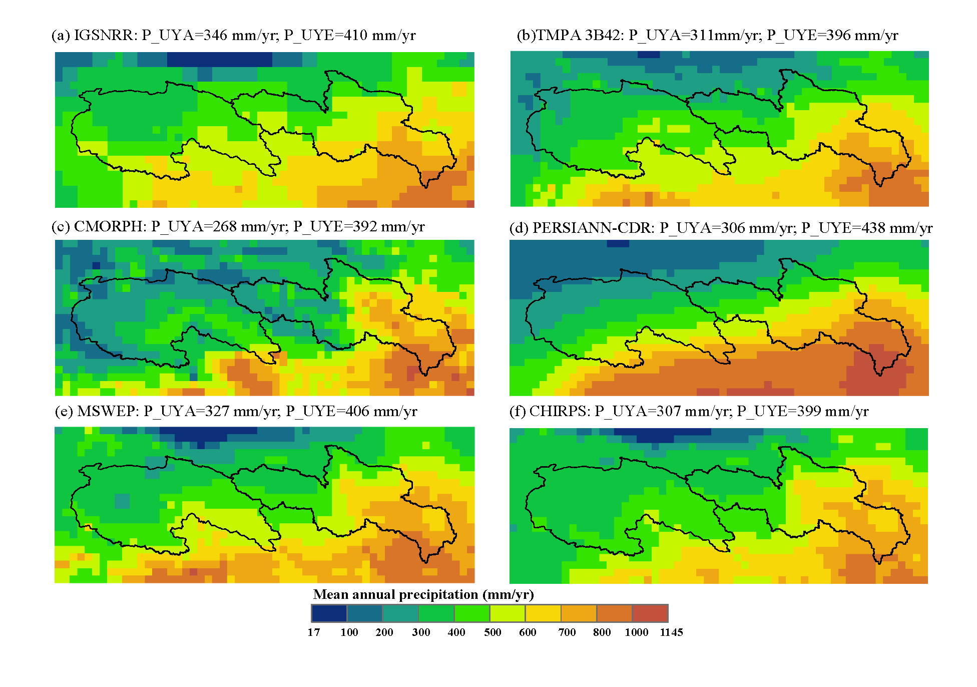
This study focuses on two gauge-scarce river basins on the TP: the source regions of the Yellow River (UYE) and Yangtze River (UYA) basins (Figure 1). The two basins are located on the northern TP and have large spatial heterogeneities in the terrain and climate within each basin. The UYE and UYA cover areas of 121,972 km2 and 137,704 km2, respectively. The total area of the two basins accounts for ~10.4% of the TP. The elevations of the two basins range from 2776 to 6313 m a.s.l. The climate conditions of the two basins are mainly dominated by the Asian monsoon [49]. The annual mean precipitation decreases as the latitude increases, and more than 70% of the precipitation occurs during the wet season (from May to September). The two basins have long-term daily streamflow records, allowing us to evaluate the capacity of hydrological modeling for different satellite precipitation products. The distribution of the meteorological stations in the two basins is very sparse and uneven. There are only four and nine stations located in the UYA and the UYE basins, respectively (Figure 1). Thus, it is difficult to characterize the realistic spatial–temporal variability in precipitation by using the interpolated precipitation data from gauge observations.
The daily streamflow records were obtained from the Hydrological Bureau of the Ministry of Water Resources of China. The daily meteorological data come from 21 national meteorological stations, which have been subject to strict quality control by the China Meteorological Administration (CMA) (http://data.cma.cn/).
2.2. Satellite Precipitation Products
In this study, five satellite precipitation products were employed, which are version 2.0 of the Climate Hazards group Infrared Precipitation with Stations (CHIRPS v2.0), CMORPH v1.0, PERSIANN-CDR, TMPA 3B42 v7, and version 2.0 of the Multi-Source Weighted-Ensemble Precipitation (MSWEP v2.0) (see Table 1). All the products incorporate satellite precipitation information with (a) gauge-based dataset(s) and have the same spatial resolution (i.e., 0.25° × 0.25°), of which the CHIRPS v2.0 and MSWEP v2.0 products also include the reanalysis data during the process of product generation [39,50]. It is worth noting that the selected five precipitation products are not completely independent: different satellite products may employ the same sensor as a data source and one product may be merged into another product. More information on the data sources of different products are given in Sun et al. (2018). The intercomparison and evaluation of these precipitation products were performed over the period 1998–2012.
CHIRPS v2.0 is a quasi-global (−50° to 50°) precipitation product that combines a pentadal precipitation climatology, geostationary thermal infrared (TIR) observations, atmospheric reanalysis, and rainfall fields and precipitation measurements from more than 20,000 gauges globally [50,51]. This product has been evaluated at a regional (e.g., Poméon, et al. [38]) and a global (e.g., Beck, et al. [39]) scale and showed reliable performance. CMORPH combines the advantages of the passive MW sensors and IR sensors and utilizes the IR-derived motion vectors to propagate the spatial–temporal resolution of the passive MW-derived precipitation estimates [23]. It has been shown to be superior to other satellite precipitation products in many regions of the world, including China [52,53]. PERSIANN-CDR uses the archive of Gridded Satellite (GridSat-B1) infrared radiation data as the input to the PERSIANN model. The model outputs are then corrected by the monthly Global Precipitation Climatology Project (GPCP) precipitation product to reduce the biases in the estimated precipitation [35,54]. PERSIANN-CDR was reported to be consistent with the ground-based precipitation product in China [35]. TRMM aims to provide the “best” estimate of quasi-global precipitation, which is equipped with multiple rainfall sensors, including a precipitation radar, a TRMM microwave imager, and a visible and infrared radiometer [22,27]. It was developed originally for rainfall retrievals in the tropics and has been extended to a quasi-global scale [38]. TRMM provides two forms of precipitation products: a near real-time product with a delay of several hours from the observation time and a gauge-adjusted product with a delay of 2–3 months from the observation time. In general, the near real-time product is more useful than the gauge-adjusted product in hydrological and meteorological operations, while the gauge-adjusted product is more accurate than the near real-time product in precipitation estimates and is mainly used for scientific research. TMPA 3B42 v7 is one of the precipitation products obtained from TRMM merged with other satellite estimates, which has wide applications at middle and low latitudes [37,55,56]. MSWEP is a newly developed global merging precipitation product that takes advantage of the strengths of gauge-, satellite-, and reanalysis-based data. This product merges five satellite-based, three reanalysis-based, and two gauge-based precipitation products during the data generation process [57]. A notable feature of the MSWEP is that it considers the gauge under-catch and orographic effects on precipitation estimates using a Budyko-based framework and global-coverage runoff observations. MSWEP has been evaluated on a global scale with 21 other precipitation products and exhibited the best performance overall [39]. For comparison purposes, a China-wide gauge-based precipitation dataset (namely, IGSNRR) was also used, aiming to test whether the satellite precipitation products outperform gauge-based precipitation in hydrological modeling of gauge-scarce regions. The IGSNRR dataset was interpolated using ~800 national meteorological stations (including the 21 stations showed in Figure 1) from the CMA [58].
3. Methodology
3.1. Hydrological Model
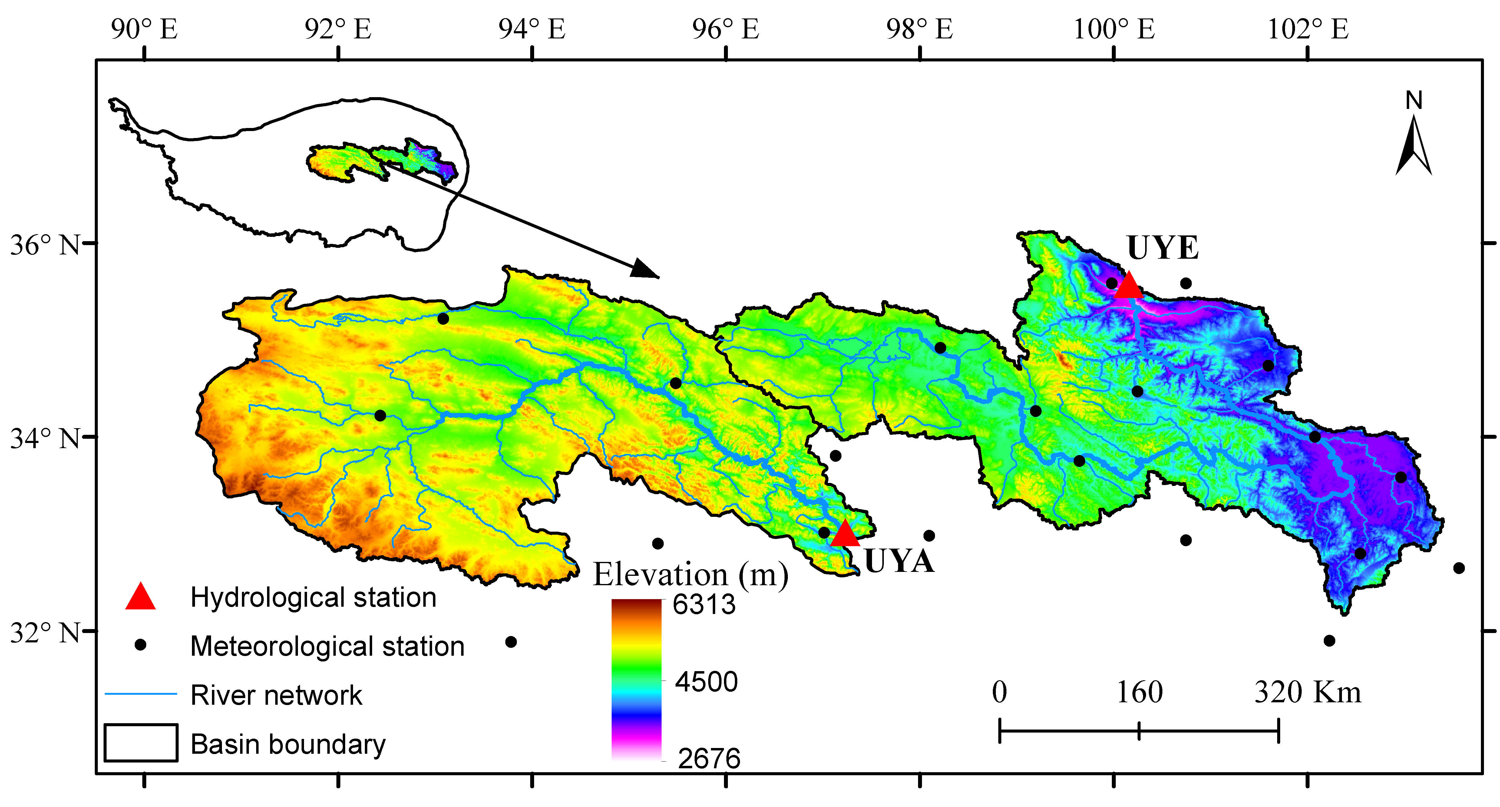
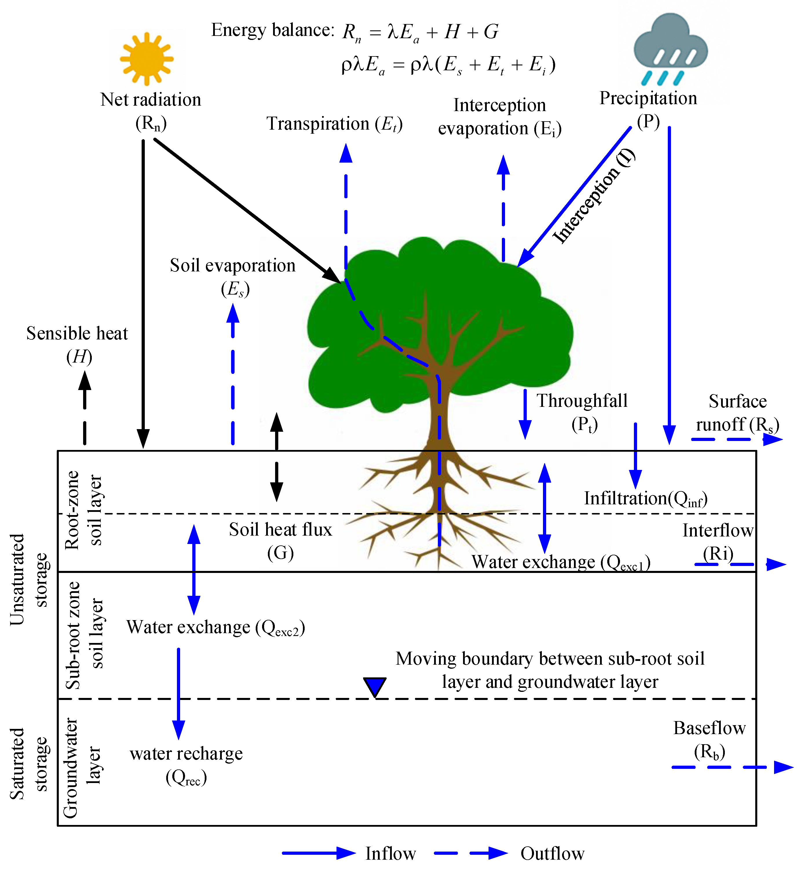
Model choices may influence the results of a hydrological evaluation. Compared with a lumped model, a distributed hydrological model can reflect the influences of spatial variability in precipitation on hydrological simulations and thus is more sensitive to the errors in precipitation inputs than a lumped model [59]. Here, the hydrological evaluation was performed via a grid-based distributed hydrological model, namely, the Hydro-Informatic Modeling System (HIMS) [10,60,61]. The HIMS model is a conceptual, process-based hydrological model that includes key hydrological processes in both the vertical and horizontal directions, including snow accumulation melt, evaporation from soil and plants, infiltration, water exchange between soil layers, and groundwater recharge and baseflow (Figure 2). The model runs on a daily scale and has a variable spatial resolution. The current version of the HIMS incorporates a temperature-based snow-accounting model, namely, CemaNeige [62], to calculate the snow accumulation and melt. The CemaNeige model has been compared with six other snow-accounting models on a large set of catchments and exhibited the best performance [62]. The HIMS model uses a physical-based Peman–Monteith (PM) equation to calculate the evaporation from soil and plants. Multiple forms of the PM equation have been developed, and the difference between them lies mainly in how to parameterize the surface conductance (i.e., the inverse of the surface resistance). In the HIMS model, the surface conductance formula developed by Leuning, et al. [63] was used, which has been reported to be superior to the empirical evaporation equation for hydrological modeling [64,65]. The model includes three runoff components: surface runoff, interflow, and baseflow. The surface runoff is calculated using a power-function infiltration equation. This equation contains both infiltration excess and saturation excess runoff mechanisms and has wide applicability [66]. The interflow and baseflow are computed via the linear reservoir method. The model has two interconnected storage units that contribute to the vertical water transfer balance: an unsaturated layer and a saturated layer. The interactions between the unsaturated and saturated layers are represented by a moving boundary in response to the groundwater storage dynamics. The horizontal water transfer is calculated based on a unit-based routing equation. The HIMS model includes 12 free parameters, which are calibrated using the observed streamflow data based on a Monte-Carlo-based calibration method [67]. The model was calibrated for each precipitation product using 10,000 parameter sets from the Monte Carlo random sampling. The observed streamflow data from 1998 to 2005 were used for the calibration, and the data from 2006 to 2012 were used for validation. The forcing data of the HIMS model mainly include the conventional meteorological variables (precipitation, temperature, relative humidity, wind speed, and sunshine duration) and land surface information (digital elevation model (DEM), land use data, leaf area index (LAI)).
3.2. Evaluation Method and Criteria
The precipitation in mountainous regions usually presents strong spatial variability [2,31]. It is difficult for an interpolated precipitation dataset from a sparse gauge network to represent the realistic spatial pattern of precipitation at the basin scale. Thus, the validations of the precipitation products were not performed at the basin scale due to a lack of reliable references. In this study, the evaluations of the precipitation products were conducted in two steps. First, a point-to-pixel validation was conducted by comparing precipitation estimates and gauge observations on a daily scale. Then, the gauge-based dataset and the five precipitation products were separately used as the precipitation forcing of the hydrological model to further assess their capacity in hydrological modeling. Four statistical metrics were selected, namely, the Pearson correlation coefficient (CC, −1 ≤ CC ≤1), percent bias (PBIAS, -∞< PBIAS < +∞), root-mean-square error (RMSE, 0 ≤ RMSE < ∞), and Kling–Gupta efficiency (KGE, −∞ < KGE ≤ 1) [68]. The CC is a measure of the strength and direction of the linear relationship between simulations and observations. The PBIAS and RMSE were used to demonstrate the error and bias between the precipitation (streamflow) estimates and gauge observations. The KGE measures the overall goodness of fit between the observations and simulations. The expressions of these performance statistics are given as:
where and are the simulations and observations, respectively, and N is the sample size. μs and σs are the mean and standard deviation of the simulations, respectively; μo and σo are the mean and standard deviation of the observations, respectively; and r is the correlation coefficient between the observations and simulations. The optimal values for the four statistical metrics are CC = 1, RMSE = 0, PBIAS = 0%, and KGE = 1. Note that a negative value of PBIAS indicates the observations being overestimated by the simulations, and vice versa [69].
4. Results
4.1. Inter-Comparison of Precipitation Products
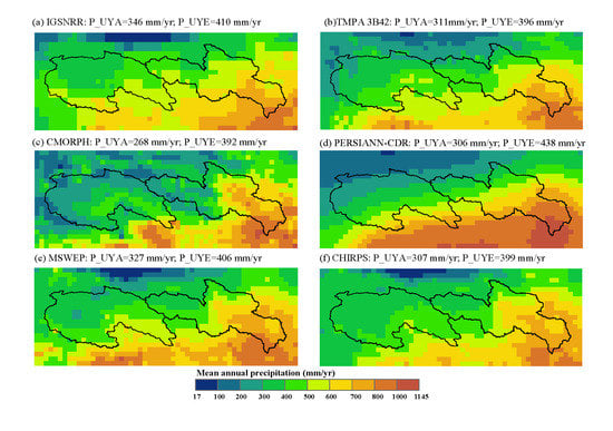
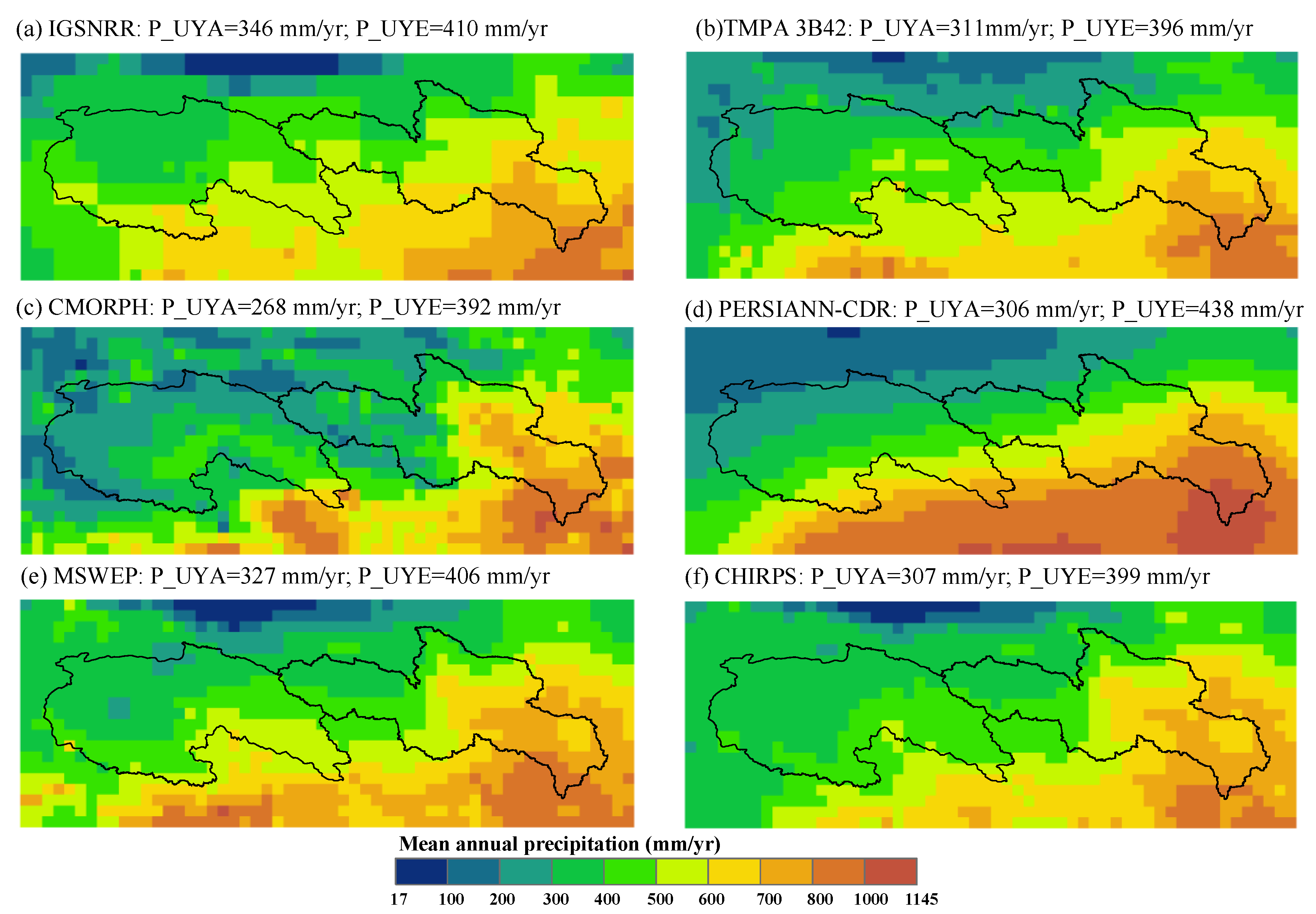
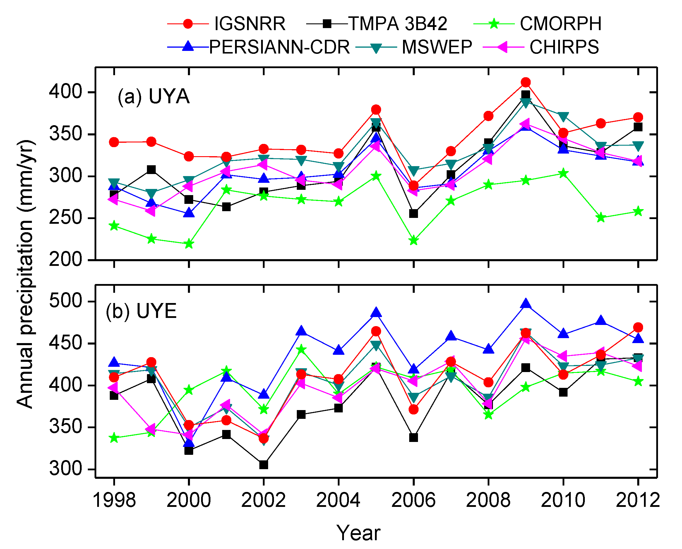
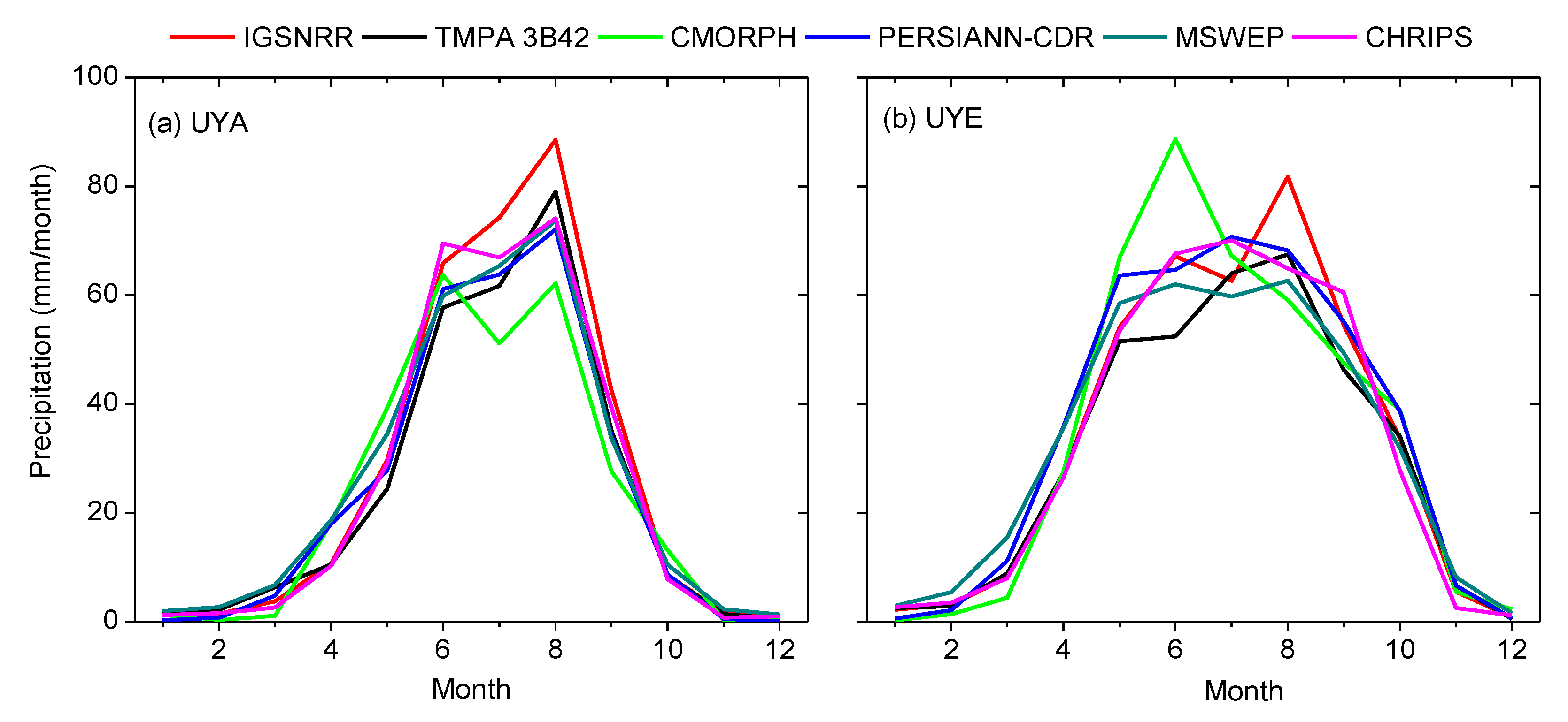
The inter-comparison of satellite precipitation products with each other can help to identify the consistency and discrepancy in precipitation estimates among the satellite products. Figure 3 shows the spatial–temporal distributions of the five precipitation products. Overall, the spatial patterns of the mean annual precipitation from these products are similar to each other, showing a decreasing trend with increasing latitude and an increasing trend with increasing longitude (Figure 3). However, the mean annual precipitation from the five precipitation products demonstrates large differences over the study area. In the UYA basin, the mean annual precipitation from the TMPA 3B42, CMORPH, PERSIANN-CDR, MSWEP, and CHIRPS is 311, 268, 306, 327, and 307 mm/yr, respectively; the values for the UYE basin are 396, 392, 438, 406, and 399 mm/yr, respectively. In addition, the time series of the basin-average annual precipitation derived from these products are also significantly different from each other (Figure 4). At a given year, in the UYA basin, the gauge-based precipitation generally has the largest values, followed by MSWEP, and CMORPH has the lowest values, while in the UYE basin, the PERSIANN precipitation generally has the largest values, and TMPA 3B42 has the lowest values in most years. In many years, the maximum difference in annual precipitation between two products is larger than 100 mm/yr. The seasonal variations in the precipitation from the five products are overall consistent with each other, except for the CMORPH product in the wet season (Figure 5). The CMORPH values are lower than the values of the other products in July and August in the UYA basin, while they are higher than the values of the other products in June in the UYE basin.
4.2. Point-to-Pixel Validation
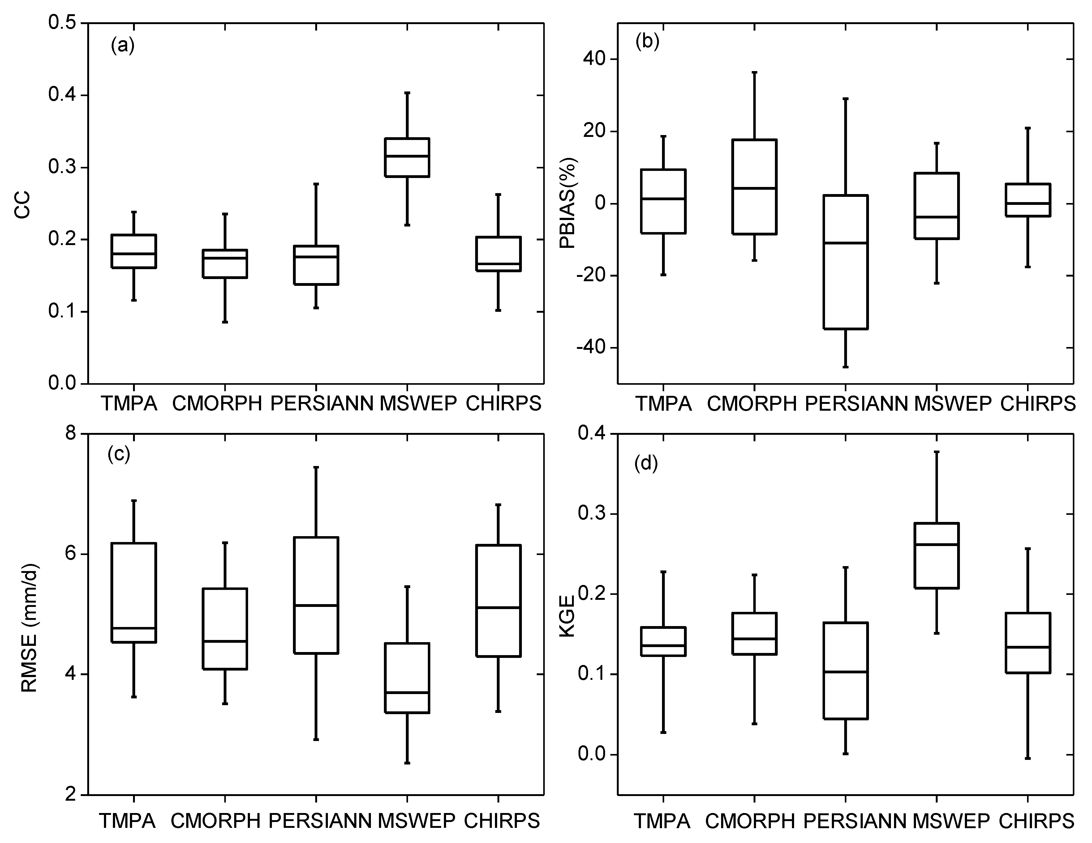
A point-to-pixel validation was performed for the five precipitation products using the daily precipitation observations from 21 meteorological stations (see Figure 1). The results are shown in Figure 6 with boxplots and Table 2. The precipitation products and gauge observations show poor linear correlations: the CC values for all products are below 0.50 at the 21 station sites. Overall, MSWEP performs better than the other products, with a median CC = 0.32, while the median CC values for the other products are similar to each other, ranging from 0.17 to 0.18. In terms of the PBIAS, CHIRPS performs the best, followed by TMPA 3B42 and MSWEP. PERSIANN-CDR tends to overestimate precipitation compared to the gauge observations, with a median PBIAS = −11.3%, whereas the CMORPH precipitation shows systematic underestimations, with a median PBIAS = 4.5%. These products show the same performance rankings in RMSE and KGE metrics: MSWEP has the highest rank, followed by CMORPH, TMPA 3B42, CHIRPS, and PERSIANN-CDR. Overall, all products cannot efficiently reproduce the temporal variability in the gauge precipitation at the daily scale. Among the five products, MSWEP has the best consistency with the gauge observations, achieving the best performance in three out of the four metrics.
4.3. Hydrological Evaluation
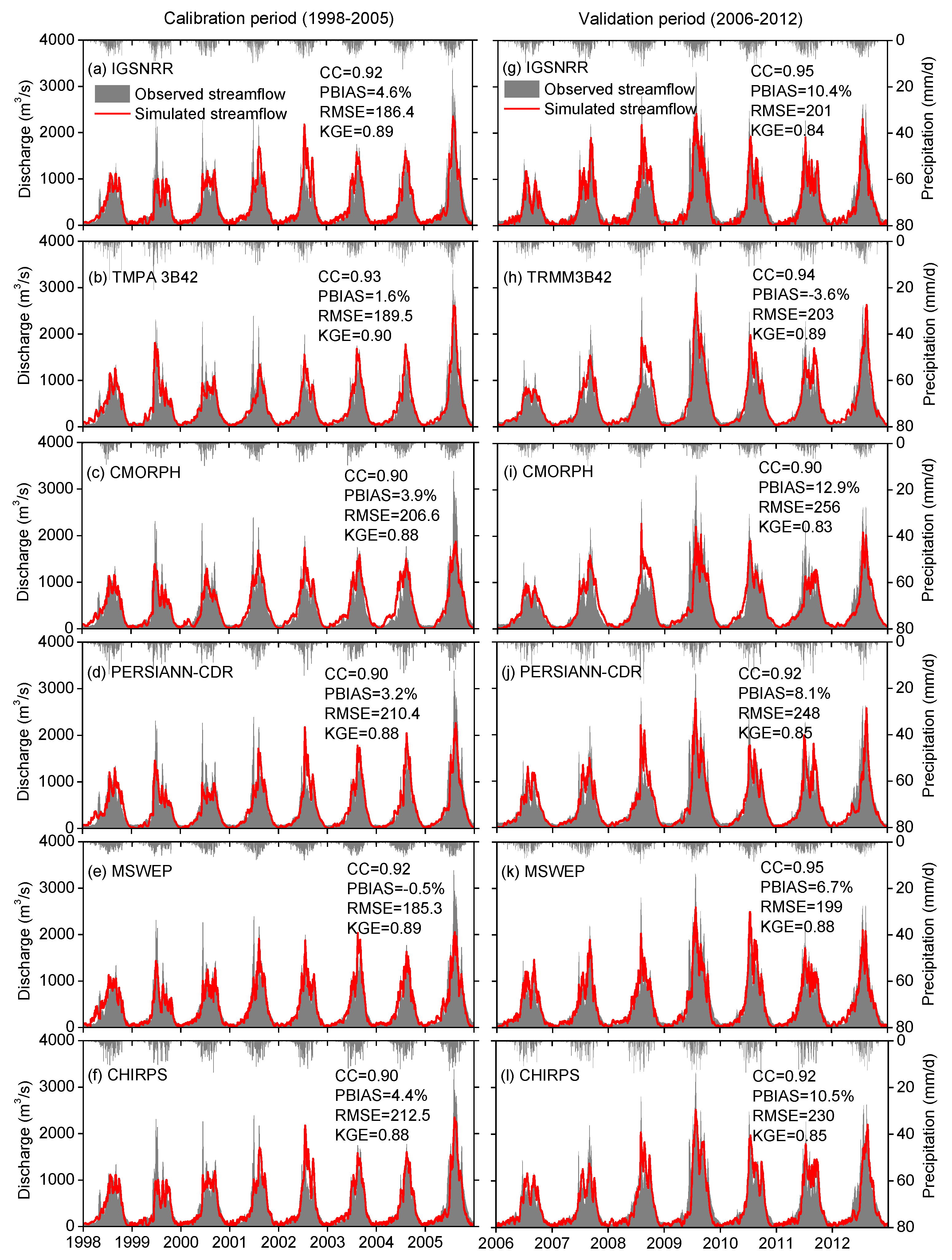
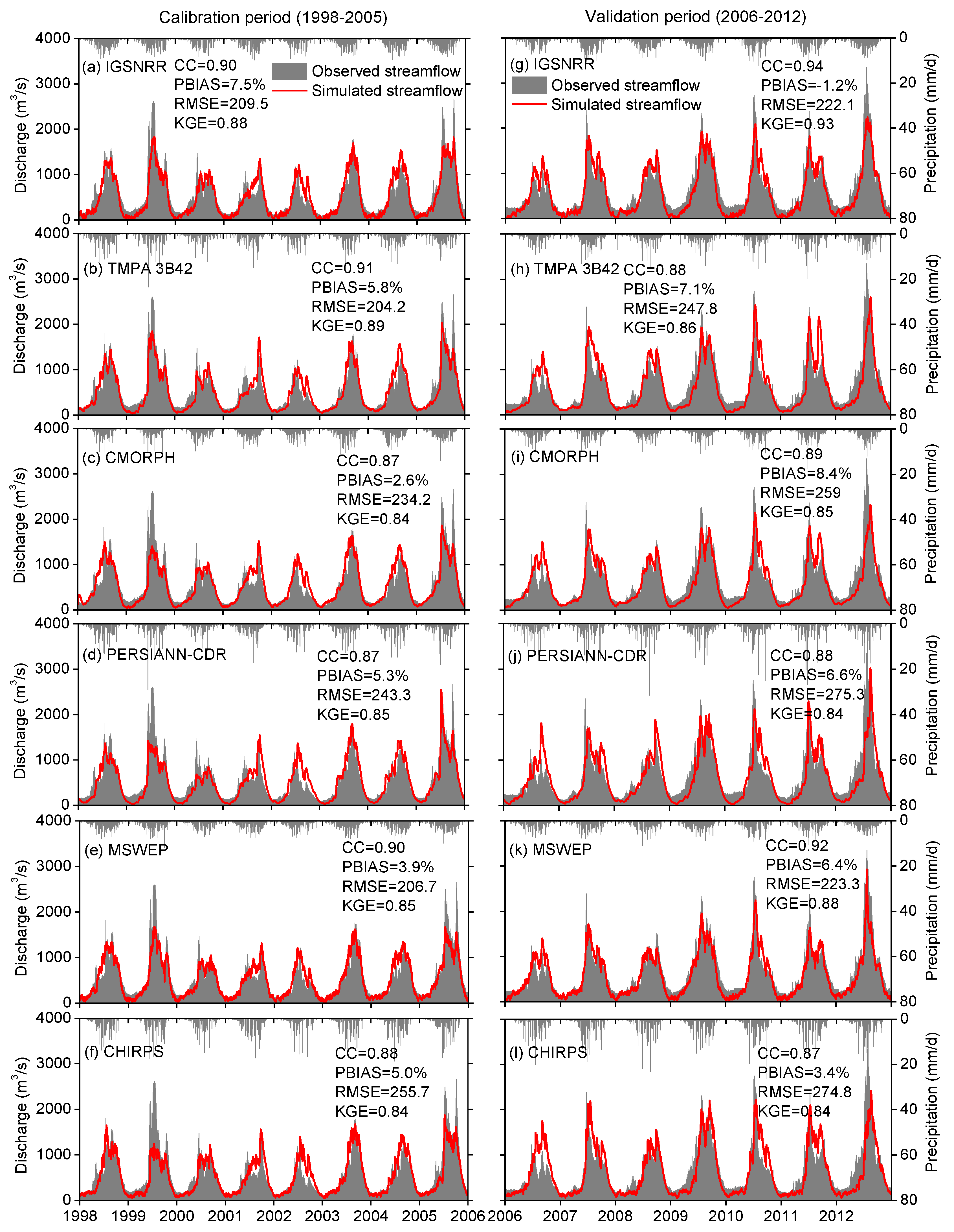
To evaluate the capacity of the streamflow simulations of the precipitation products, the HIMS model was separately calibrated using gauge-interpolated precipitation and satellite precipitation products by maximizing the KGE between the observed and simulated streamflows. Figure 7 and Figure 8 demonstrate the simulated and observed daily streamflows in the two basins during the calibration period (1998–2005) and validation period (2006–2012). Given that the model performance during the validation period better reflects the actual predictive ability of the hydrological model, hereafter, we only present the model performance during the validation period. Overall, all products used as the precipitation forcing of the HIMS model can well-reproduce the streamflow observations in the two basins. The KGE values obtained by the precipitation products are larger than 0.83 in the UYA basin and 0.84 in the UYE basin. Although significant differences in precipitation estimates exist in these products, the model performance statistics driven by the precipitation products are similar to each other. For example, in the UYA basin, the CC values obtained from TMPA 3B42, CMORPH, PERSIANN-CDR, MSWEP, and CHIRPS are 0.94, 0.90, 0.92, 0.95, and 0.92, respectively; the KGE values from these products are 0.89, 0.83, 0.85, 0.88, and 0.85, respectively. In general, no single product consistently produces the best performance among the five products. Comparatively, TMPA 3B42 and MSWEP perform better than the other products in the UYA basin. Both of them achieve the best performance in two out of the four statistical metrics. MSWEP outperforms the other products in the UYE basin, which produces the best performance in three out of the four statistical metrics.
In the UYA basin, the streamflow prediction capacity using the precipitation products was similar to or even better than that using the gauge-based precipitation dataset (i.e., IGSNRR). The KGE values obtained from the five products except for the CMORPH are larger than those obtained from IGSNRR. However, in the UYE basin, gauge-based precipitation performs better in streamflow simulations than the precipitation products, which obtains the best performance in all statistical metrics. A possible reason for the inconsistent results between the two basins is that the number of stations within the UYE basin is larger than that within the UYA basin (nine versus four); another possible reason is that the topography in the UYA basin is more complex than that in the UYE basin (Figure 1). The two reasons may result in the interpolated precipitation data in the UYE basin being more reliable than those in the UYA basin.
5. Discussion
5.1. Validation of the Satellite Precipitation Products
In this study, a point-to-pixel validation was performed by comparing the precipitation products and gauge observations directly at 21 grid boxes. The results showed that no single product agrees well with the daily gauge observations, indicating that the precipitation products are subject to larger uncertainties in daily precipitation estimates. This result is consistent with the results of previous studies by Gao and Liu [46], Tong, et al. [30], Wang, et al. [47], and Miao, et al. [35]. Several studies also found that the satellite precipitation products have larger uncertainties on the TP than in other places [36,39,53]. This is partly because few stations on the TP were involved in the calibration process of satellite precipitation products [27,36]. In addition, both IR-based and MW-based methods are tricky over high elevations and cold surfaces and suffer from the error associated with virga, i.e., precipitation evaporating before reaching the ground, which is common over arid mountainous areas. These limitations cause precipitation retrievals on the TP to be generally less accurate in capturing orographic precipitation and solid precipitation [27,36]. This may also be a reason for the poor agreement between precipitation products and gauge observations on the TP. Among these products, MSWEP generally provides the best validation results. This is probably because the MSWEP directly incorporates global-scale daily gauge data and accounts for gauge under-catch and orographic influences using larger numbers of runoff observations during the process of data generation [39]. The results also indicated that PERSIANN-CDR tends to overestimate precipitation compared with the gauge observations in the UYE basin, while systematic underestimations were found in CMORPH in the UYA basin. Similar results were also achieved by Tong, et al. [30], Gao and Liu [46], and Miao, et al. [35] for PERSIANN-CDR and CMORPH.
Note that although the validation method of the point-to-pixels has commonly been used for precipitation products [9,33,39,42,70,71], it has an inevitable deficiency due to the scale mismatch and wind-induced precipitation under-catch between the precipitation products and gauge observations. It is difficult for a single station to represent grid-wide (0.25° × 0.25°, ~625 km2) average precipitation, particularly in gauge-sparse regions, since the precipitation over complex mountainous terrain is highly variable in space. Moreover, the conventional gauge observations are also subject to the under-catch of solid precipitation under windy conditions. Under-catch errors in precipitation gauge observations can be as large as 20–90%, as reported by Yang, et al. [72], in Greenland. These deficiencies in the validation method might result in some degree of uncertainty in the validation results.
5.2. Hydrological Evaluations of the Satellite Precipitation Products
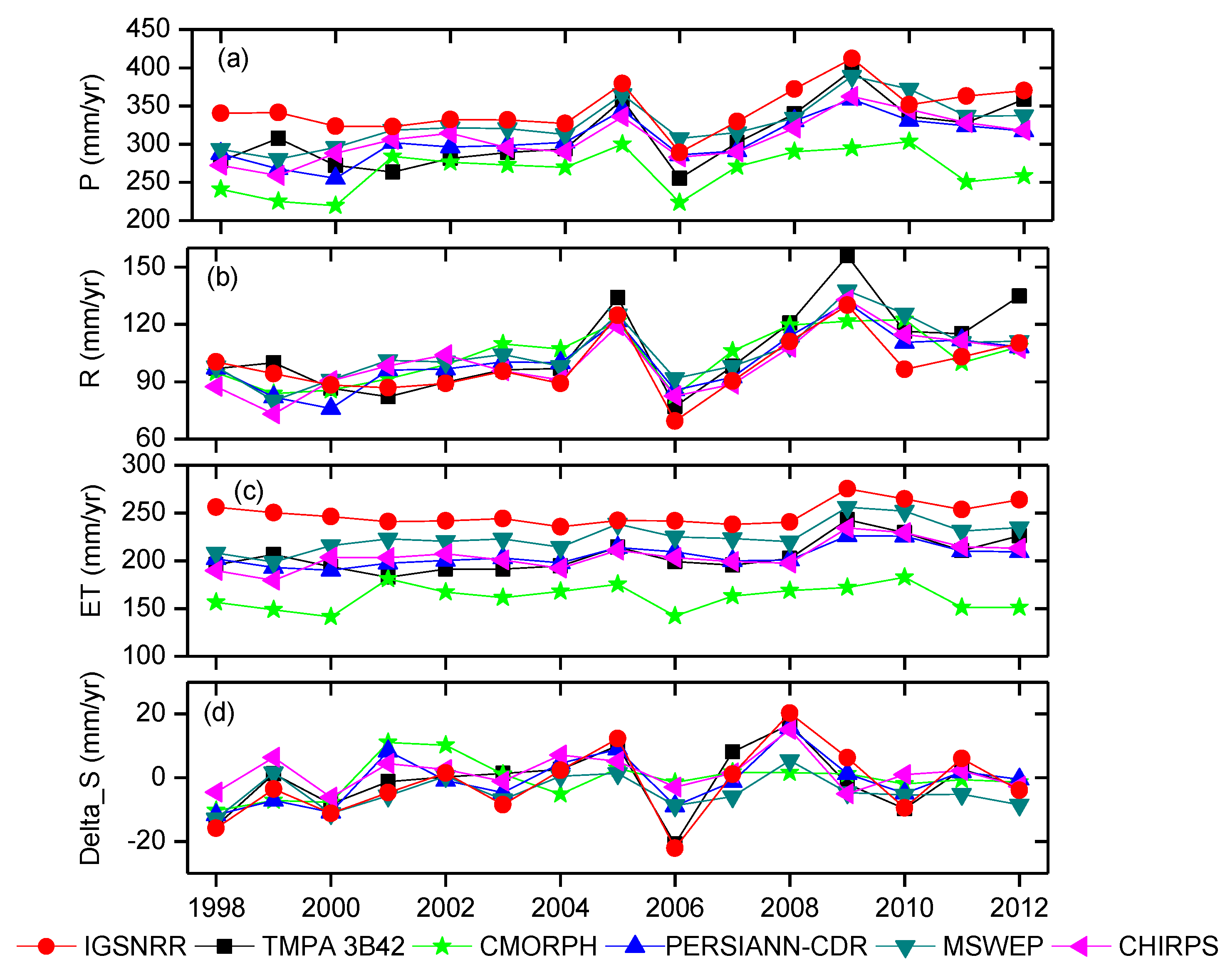
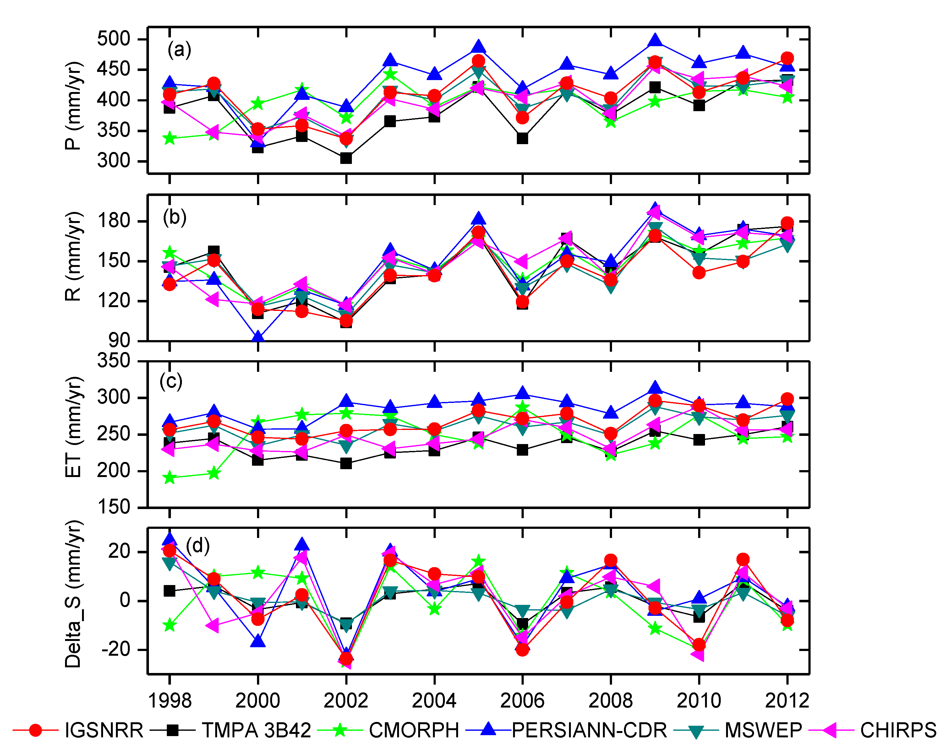
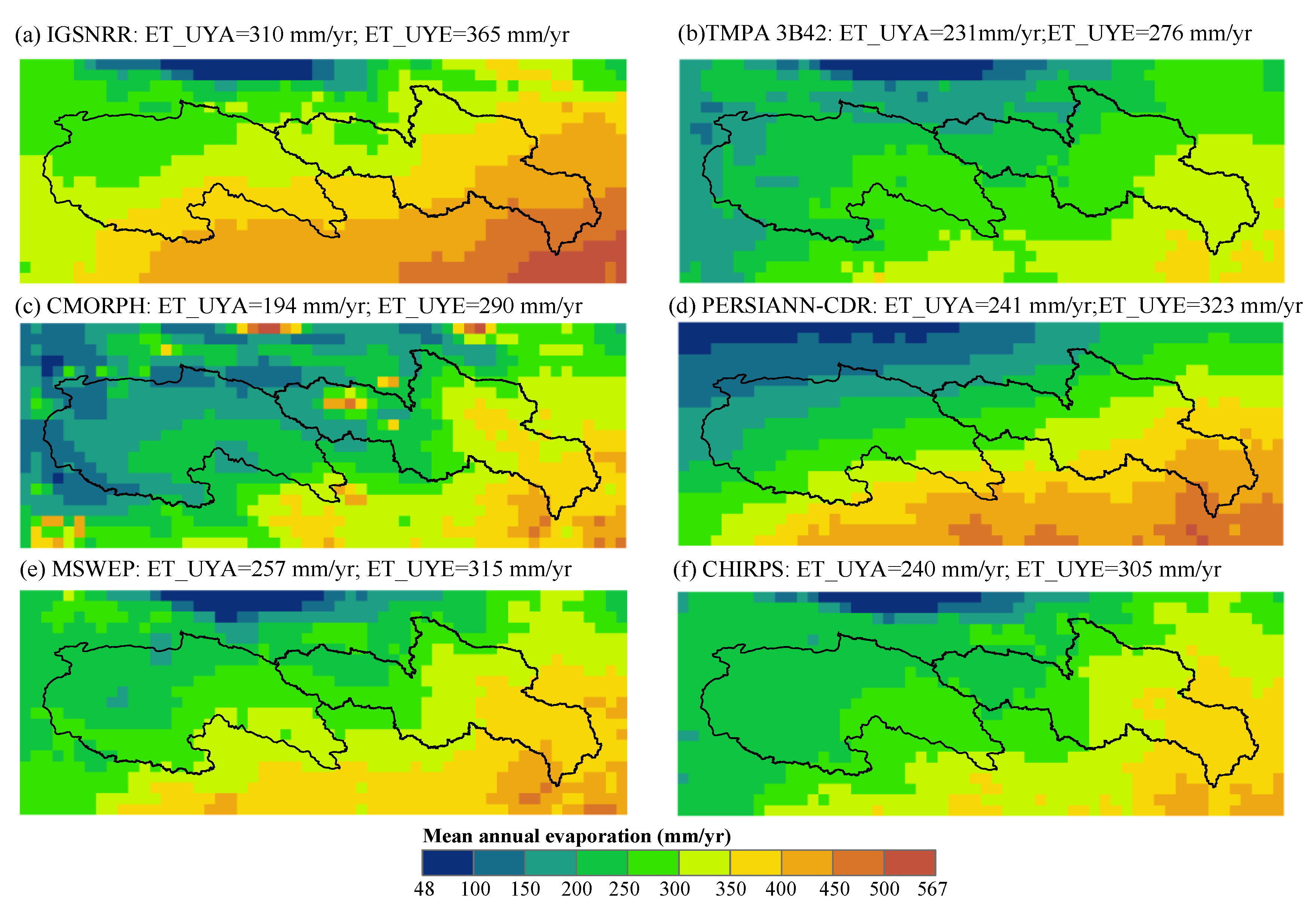
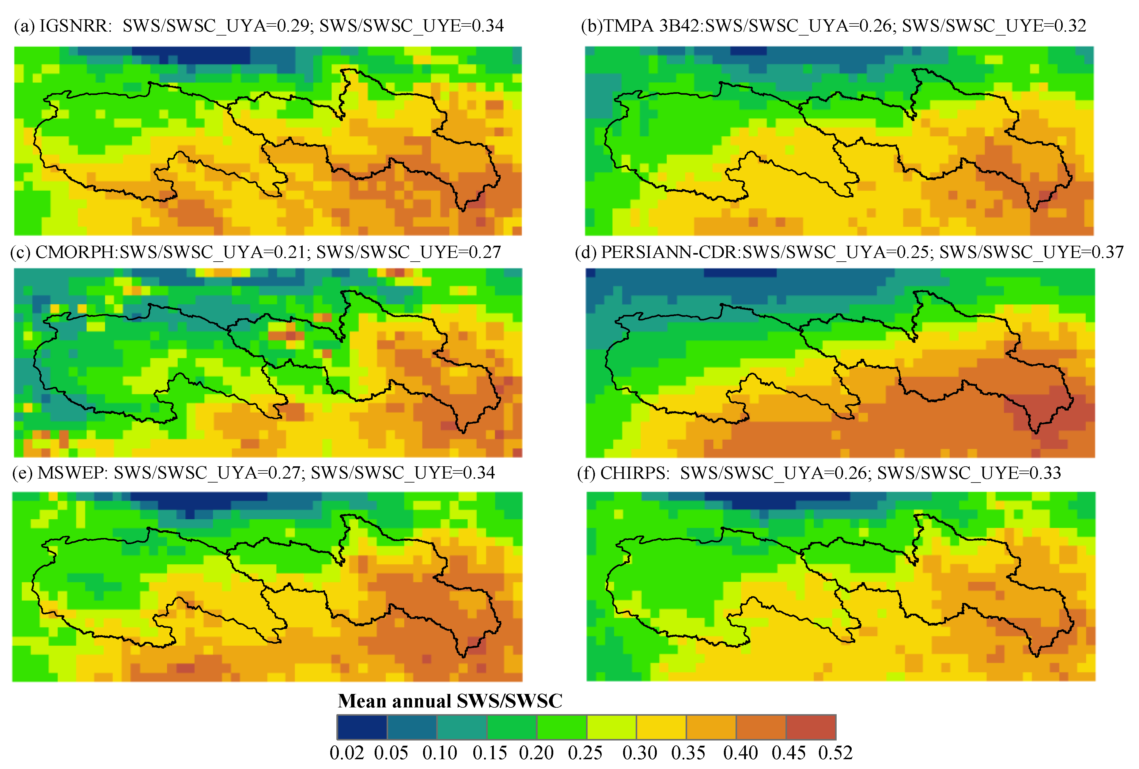
For hydrology models, errors in precipitation inputs can lead to large uncertainties in streamflow simulations and predictions [73,74,75]. The hydrological evaluations of the precipitation products are just based on the hypothesis that errors in the precipitation inputs can propagate into the hydrological simulations [26,59]. Compared with the point-to-pixel validation, evaluating precipitation products based on their predictability of streamflow is attractive, as it is performed at the basin scale and avoids the scale discrepancy problem using gauge observations for validation [38]. In this study, we compared the model performances for streamflow simulations driven by a gauge-based dataset and five precipitation products. Although there are considerable differences among these products (see Section 4.1 and Section 4.2), all products are able to accurately reproduce the observed streamflow in the study basins. A possible explanation is that the large differences in the precipitation inputs were buffered inside the hydrological model via parameter calibration. The parameter calibration based on only streamflow simulations leads to model parameters that are ‘‘falsely adjusted” to maximize the streamflow simulation performances [76], thereby compensating for the efficiency loss in the runoff simulations caused by different precipitation inputs. It should be noted that this compensation may be only valid within a certain threshold of precipitation error. Beyond this threshold, model calibration may be limitedly resistant to error propagation of precipitation products to runoff simulations. Moreover, larger basins tend to be more tolerant of the effect of precipitation error on runoff simulations than the smaller basins [16]. Nevertheless, according to the principle of water balance, the large differences in the precipitation inputs should be reflected by the simulated water balance components, except for runoff. To confirm this deduction, we compared the simulated evapotranspiration (ET), runoff (R), and water storage change (Delta_S) driven by the different precipitation (P) inputs at an annual scale (Figure 9 and Figure 10). As shown in Figure 9 and Figure 10, the changes in R, ET, and Delta_S are dominated by the changes in P; a larger P generally produces a larger ET and Delta_S. For example, the mean annual ET of IGSNRR is approximately 1.5-fold higher than that of CMORPH in the UYA basin; the maximum difference in the annual ET between PERSIANN-CDR and TMPA 3B42 reaches 83.6 mm in the UYE basin. The Delta_S values demonstrate smaller differences than the ET values between these products, and the magnitude of change varies from −30 to 30 mm in the two basins. The spatial patterns of ET and relative soil water storage (SWS/SWSC, see the caption of Figure 11) are also similar to those of precipitation (Figure 11 and Figure 12). The above results confirm that the parameter calibration greatly offsets the influences of different precipitation inputs on streamflow simulations by adjusting the ET and Delta_S. Thus, hydrological evaluations of the precipitation products regarding only the streamflow simulations are less meaningful. In contrast, an efficient hydrological evaluation for precipitation products should focus on both streamflow simulations and the simulations of other hydrological variables, such as evaporation and soil moisture. Similarly, the calibration of hydrological models should also include additional constrains in addition to runoff to improve the physical realism of hydrological models [76].
6. Conclusions
The ground-based precipitation observation networks are extremely sparse over the TP, which is challenging for hydrological studies and applications in this region. In this study, five satellite precipitation products were evaluated through gauge observations and the accuracy of streamflow simulations. The main conclusions are summarized as follows:
- The used precipitation products showed similar spatial patterns but considerable differences in the precipitation amount estimates, and suffer from large uncertainties in the daily precipitation estimates compared to the rain gauge observations. Among the five products, MSWEP shows the best consistency with the gauge observations. We thus recommend this product as the preferred choice for applications among the five products.
- All used precipitation products are able to accurately reproduce the observed streamflow hydrographs by parameter calibration of the hydrological model. However, the differences in precipitation inputs inevitably reflect on the simulations of other hydrological variables other than runoff, e.g., evaporation and water storage, leading to significantly different estimates for these variables.
- Evaluation of precipitation products regarding only the accuracy of streamflow simulations will mask the differences between these products, since the hydrological models have the ability to buffer the influences of different precipitation inputs on streamflow simulations by parameter calibration.
Similarly, the calibration of hydrological models using streamflow data alone is likely insufficient to well-simulate the hydrological variables in addition to runoff. This calibration strategy is like a “double-edged sword”, which may cause other hydrological variables other than runoff to be incorrectly simulated while improving the accuracy of runoff simulations. In addition, although the satellite precipitation products have limitations in the accuracy of precipitation estimates, they demonstrated good potential for hydrological studies and applications in our case study on the TP. The future development of satellite precipitation products should combine the advantages of the satellite and ground-based observations and reanalysis data.
Author Contributions
P.B. performed the research design, analyzed the data and wrote the draft; X.L. edited the draft and provided constructive suggestions to improve the paper.
Funding
This research was supported by the National Key Research and Development Program of China (No. 2016YFC0401402) and the Natural Science Foundation of China (No. 41601034, 41330529, and 41571024).
Acknowledgments
The authors appreciate all the providers of precipitation products to allow us download the precipitation datasets for free; we would also like to thank the reviewers and editors who provided valuable comments and suggestions for this paper.
Conflicts of Interest
The authors declare no conflict of interest.
References
- Vergara, H.; Hong, Y.; Gourley, J.J.; Anagnostou, E.N.; Maggioni, V.; Stampoulis, D.; Kirstetter, P.-E. Effects of Resolution of Satellite-Based Rainfall Estimates on Hydrologic Modeling Skill at Different Scales. J. Hydrometeorol. 2014, 15, 593–613. [Google Scholar] [CrossRef]
- Ward, E.; Buytaert, W.; Peaver, L.; Wheater, H. Evaluation of precipitation products over complex mountainous terrain: A water resources perspective. Adv. Water Resour. 2011, 34, 1222–1231. [Google Scholar] [CrossRef]
- Borga, M.; Stoffel, M.; Marchi, L.; Marra, F.; Jakob, M. Hydrogeomorphic response to extreme rainfall in headwater systems: Flash floods and debris flows. J. Hydrol. 2014, 518, 194–205. [Google Scholar] [CrossRef]
- Norbiato, D.; Borga, M.; Degli Esposti, S.; Gaume, E.; Anquetin, S. Flash flood warning based on rainfall thresholds and soil moisture conditions: An assessment for gauged and ungauged basins. J. Hydrol. 2008, 362, 274–290. [Google Scholar] [CrossRef]
- Marra, F.; Nikolopoulos, E.I.; Creutin, J.D.; Borga, M. Radar rainfall estimation for the identification of debris-flow occurrence thresholds. J. Hydrol. 2014, 519, 1607–1619. [Google Scholar] [CrossRef]
- Miao, C.; Kong, D.; Wu, J.; Duan, Q. Functional degradation of the water–sediment regulation scheme in the lower Yellow River: Spatial and temporal analyses. Sci. Total Environ. 2016, 551, 16–22. [Google Scholar] [CrossRef] [PubMed]
- Zhang, D.; Zhang, Q.; Qiu, J.; Bai, P.; Liang, K.; Li, X. Intensification of hydrological drought due to human activity in the middle reaches of the Yangtze River, China. Sci. Total Environ. 2018, 637–638, 1432–1442. [Google Scholar] [CrossRef] [PubMed]
- Liu, X.; Liu, C.; Brutsaert, W. Investigation of a Generalized Nonlinear Form of the Complementary Principle for Evaporation Estimation. J. Geophys. Res. Atmos. 2018, 123, 3933–3942. [Google Scholar] [CrossRef]
- Ashouri, H.; Nguyen, P.; Thorstensen, A.; Hsu, K.-L.; Sorooshian, S.; Braithwaite, D. Assessing the Efficacy of High-Resolution Satellite-Based PERSIANN-CDR Precipitation Product in Simulating Streamflow. J. Hydrometeorol. 2016, 17, 2061–2076. [Google Scholar] [CrossRef]
- Liu, X.; Yang, T.; Hsu, K.; Liu, C.; Sorooshian, S. Evaluating the streamflow simulation capability of PERSIANN-CDR daily rainfall products in two river basins on the Tibetan Plateau. Hydrol. Earth Syst. Sci. 2017, 21, 169–181. [Google Scholar] [CrossRef] [Green Version]
- Thiemig, V.; Rojas, R.; Zambrano-Bigiarini, M.; Levizzani, V.; De Roo, A. Validation of Satellite-Based Precipitation Products over Sparsely Gauged African River Basins. J. Hydrometeorol. 2012, 13, 1760–1783. [Google Scholar] [CrossRef] [Green Version]
- Li, H.; Hong, Y.; Xie, P.; Gao, J.; Niu, Z.; Kirstetter, P.; Yong, B. Variational merged of hourly gauge-satellite precipitation in China: Preliminary results. J. Geophys. Res. Atmos. 2015, 120, 9897–9915. [Google Scholar] [CrossRef] [Green Version]
- Germann, U.; Joss, J. Mesobeta Profiles to Extrapolate Radar Precipitation Measurements above the Alps to the Ground Level. J. Appl. Meteorol. 2002, 41, 542–557. [Google Scholar] [CrossRef]
- Wilson, J.W.; Brandes, E.A. Radar Measurement of Rainfall—A Summary. Bull. Am. Meteorol. Soc. 1979, 60, 1048–1060. [Google Scholar] [CrossRef]
- Price, K.; Purucker, S.T.; Kraemer, S.R.; Babendreier, J.E.; Knightes, C.D. Comparison of radar and gauge precipitation data in watershed models across varying spatial and temporal scales. Hydrol. Process. 2014, 28, 3505–3520. [Google Scholar] [CrossRef]
- Mei, Y.; Nikolopoulos, E.; Anagnostou, E.; Zoccatelli, D.; Borga, M. Error Analysis of Satellite Precipitation-Driven Modeling of Flood Events in Complex Alpine Terrain. Remote Sens. 2016, 8, 293. [Google Scholar] [CrossRef]
- Gottardi, F.; Obled, C.; Gailhard, J.; Paquet, E. Statistical reanalysis of precipitation fields based on ground network data and weather patterns: Application over French mountains. J. Hydrol. 2012, 432–433, 154–167. [Google Scholar] [CrossRef]
- Marra, F.; Morin, E.; Peleg, N.; Mei, Y.; Anagnostou, E.N. Intensity–duration–frequency curves from remote sensing rainfall estimates: Comparing satellite and weather radar over the eastern Mediterranean. Hydrol. Earth Syst. Sci. 2017, 21, 2389–2404. [Google Scholar] [CrossRef]
- Cohen Liechti, T.; Matos, J.P.; Boillat, J.L.; Schleiss, A.J. Comparison and evaluation of satellite derived precipitation products for hydrological modeling of the Zambezi River Basin. Hydrol. Earth Syst. Sci. 2012, 16, 489–500. [Google Scholar] [CrossRef] [Green Version]
- Lauri, H.; Räsänen, T.A.; Kummu, M. Using Reanalysis and Remotely Sensed Temperature and Precipitation Data for Hydrological Modeling in Monsoon Climate: Mekong River Case Study. J. Hydrometeorol. 2014, 15, 1532–1545. [Google Scholar] [CrossRef]
- Tobin, K.J.; Bennett, M.E. Adjusting Satellite Precipitation Data to Facilitate Hydrologic Modeling. J. Hydrometeorol. 2010, 11, 966–978. [Google Scholar] [CrossRef]
- Huffman, G.J.; Bolvin, D.T.; Nelkin, E.J.; Wolff, D.B.; Adler, R.F.; Gu, G.; Hong, Y.; Bowman, K.P.; Stocker, E.F. The TRMM Multisatellite Precipitation Analysis (TMPA): Quasi-Global, Multiyear, Combined-Sensor Precipitation Estimates at Fine Scales. J. Hydrometeorol. 2007, 8, 38–55. [Google Scholar] [CrossRef]
- Joyce, R.J.; Janowiak, J.E.; Arkin, P.A.; Xie, P. CMORPH: A Method that Produces Global Precipitation Estimates from Passive Microwave and Infrared Data at High Spatial and Temporal Resolution. J. Hydrometeorol. 2004, 5, 487–503. [Google Scholar] [CrossRef]
- Sorooshian, S.; Hsu, K.-L.; Gao, X.; Gupta, H.V.; Imam, B.; Braithwaite, D. Evaluation of PERSIANN System Satellite-Based Estimates of Tropical Rainfall. Bull. Am. Meteorol. Soc. 2000, 81, 2035–2046. [Google Scholar] [CrossRef]
- Huffman, G.J.; Bolvin, D.T.; Braithwaite, D.; Hsu, K.L.; Joyce, R.; Xie, P. NASA Global Precipitation Measurement (GPM) Integrated Multi-Satellite Retrievals for GPM (IMERG); Algorithm Theor. Basis Doc. (ATBD) Version 5.1; NASA GSFC: Greenbelt, MD, USA, 2014. Available online: https://pmm.nasa.gov/sites/default/files/document_files/IMERG_ATBD_V5.1b.pdf (accessed on 12 February 2018).
- Li, Z.; Yang, D.; Gao, B.; Jiao, Y.; Hong, Y.; Xu, T. Multiscale Hydrologic Applications of the Latest Satellite Precipitation Products in the Yangtze River Basin using a Distributed Hydrologic Model. J. Hydrometeorol. 2015, 16, 407–426. [Google Scholar] [CrossRef]
- Sun, Q.; Miao, C.; Duan, Q.; Ashouri, H.; Sorooshian, S.; Hsu, K.-L. A Review of Global Precipitation Data Sets: Data Sources, Estimation, and Intercomparisons. Rev. Geophys. 2018, 56, 79–107. [Google Scholar] [CrossRef] [Green Version]
- Scofield, R.A.; Kuligowski, R.J. Status and Outlook of Operational Satellite Precipitation Algorithms for Extreme-Precipitation Events. Weather Forecast. 2003, 18, 1037–1051. [Google Scholar] [CrossRef] [Green Version]
- Brown, J.E.M. An analysis of the performance of hybrid infrared and microwave satellite precipitation algorithms over India and adjacent regions. Remote Sens. Environ. 2006, 101, 63–81. [Google Scholar] [CrossRef]
- Tong, K.; Su, F.; Yang, D.; Hao, Z. Evaluation of satellite precipitation retrievals and their potential utilities in hydrologic modeling over the Tibetan Plateau. J. Hydrol. 2014, 519, 423–437. [Google Scholar] [CrossRef]
- Mei, Y.; Nikolopoulos, E.I.; Anagnostou, E.N.; Borga, M. Evaluating Satellite Precipitation Error Propagation in Runoff Simulations of Mountainous Basins. J. Hydrometeorol. 2016, 17, 1407–1423. [Google Scholar] [CrossRef]
- Su, F.; Hong, Y.; Lettenmaier, D.P. Evaluation of TRMM Multisatellite Precipitation Analysis (TMPA) and Its Utility in Hydrologic Prediction in the La Plata Basin. J. Hydrometeorol. 2008, 9, 622–640. [Google Scholar] [CrossRef]
- Yong, B.; Hong, Y.; Ren, L.-L.; Gourley, J.J.; Huffman, G.J.; Chen, X.; Wang, W.; Khan, S.I. Assessment of evolving TRMM-based multisatellite real-time precipitation estimation methods and their impacts on hydrologic prediction in a high latitude basin. J. Geophys. Res. Atmos. 2012, 117. [Google Scholar] [CrossRef] [Green Version]
- Deus, D.; Gloaguen, R.; Krause, P. Water Balance Modeling in a Semi-Arid Environment with Limited in situ Data Using Remote Sensing in Lake Manyara, East African Rift, Tanzania. Remote Sens. 2013, 5, 1651–1680. [Google Scholar] [CrossRef] [Green Version]
- Miao, C.; Ashouri, H.; Hsu, K.-L.; Sorooshian, S.; Duan, Q. Evaluation of the PERSIANN-CDR Daily Rainfall Estimates in Capturing the Behavior of Extreme Precipitation Events over China. J. Hydrometeorol. 2015, 16, 1387–1396. [Google Scholar] [CrossRef]
- Yong, B.; Liu, D.; Gourley, J.J.; Tian, Y.; Huffman, G.J.; Ren, L.; Hong, Y. Global View Of Real-Time Trmm Multisatellite Precipitation Analysis: Implications for Its Successor Global Precipitation Measurement Mission. Bull. Am. Meteorol. Soc. 2015, 96, 283–296. [Google Scholar] [CrossRef]
- Tang, G.; Zeng, Z.; Long, D.; Guo, X.; Yong, B.; Zhang, W.; Hong, Y. Statistical and Hydrological Comparisons between TRMM and GPM Level-3 Products over a Midlatitude Basin: Is Day-1 IMERG a Good Successor for TMPA 3B42V7? J. Hydrometeorol. 2016, 17, 121–137. [Google Scholar] [CrossRef]
- Poméon, T.; Jackisch, D.; Diekkrüger, B. Evaluating the performance of remotely sensed and reanalysed precipitation data over West Africa using HBV light. J. Hydrol. 2017, 547, 222–235. [Google Scholar] [CrossRef]
- Beck, H.E.; Vergopolan, N.; Pan, M.; Levizzani, V.; van Dijk, A.I.J.M.; Weedon, G.P.; Brocca, L.; Pappenberger, F.; Huffman, G.J.; Wood, E.F. Global-scale evaluation of 22 precipitation datasets using gauge observations and hydrological modeling. Hydrol. Earth Syst. Sci. 2017, 21, 6201–6217. [Google Scholar] [CrossRef] [Green Version]
- Mei, Y.; Anagnostou, E.N.; Shen, X.; Nikolopoulos, E.I. Decomposing the satellite precipitation error propagation through the rainfall-runoff processes. Adv. Water Resour. 2017, 109, 253–266. [Google Scholar] [CrossRef]
- Mei, Y.; Anagnostou, E.N.; Nikolopoulos, E.I.; Borga, M. Error Analysis of Satellite Precipitation Products in Mountainous Basins. J. Hydrometeorol. 2014, 15, 1778–1793. [Google Scholar] [CrossRef]
- Tong, K.; Su, F.; Yang, D.; Zhang, L.; Hao, Z. Tibetan Plateau precipitation as depicted by gauge observations, reanalyses and satellite retrievals. Int. J. Clim. 2014, 34, 265–285. [Google Scholar] [CrossRef]
- Bai, P.; Liu, X.; Yang, T.; Liang, K.; Liu, C. Evaluation of streamflow simulation results of land surface models in GLDAS on the Tibetan plateau. J. Geophys. Res. Atmos. 2016, 121, 12180–12197. [Google Scholar] [CrossRef]
- Xu, R.; Tian, F.; Yang, L.; Hu, H.; Lu, H.; Hou, A. Ground validation of GPM IMERG and TRMM 3B42V7 rainfall products over southern Tibetan Plateau based on a high-density rain gauge network. J. Geophys. Res. Atmos. 2017, 122, 910–924. [Google Scholar] [CrossRef]
- Bennartz, R.; Michelson, D.B. Correlation of precipitation estimates from spaceborne passive microwave sensors and weather radar imagery for BALTEX PIDCAP. Int. J. Remote Sens. 2003, 24, 723–739. [Google Scholar] [CrossRef]
- Gao, Y.C.; Liu, M.F. Evaluation of high-resolution satellite precipitation products using rain gauge observations over the Tibetan Plateau. Hydrol. Earth Syst. Sci. 2013, 17, 837–849. [Google Scholar] [CrossRef] [Green Version]
- Wang, S.; Liu, S.; Mo, X.; Peng, B.; Qiu, J.; Li, M.; Liu, C.; Wang, Z.; Bauer-Gottwein, P. Evaluation of Remotely Sensed Precipitation and Its Performance for Streamflow Simulations in Basins of the Southeast Tibetan Plateau. J. Hydrometeorol. 2015, 16, 2577–2594. [Google Scholar] [CrossRef]
- Yan, D.; Liu, S.; Qin, T.; Weng, B.; Li, C.; Lu, Y.; Liu, J. Evaluation of TRMM precipitation and its application to distributed hydrological model in Naqu River Basin of the Tibetan Plateau. Hydrol. Res. 2017, 48, 822–839. [Google Scholar] [CrossRef]
- Yao, T.; Thompson, L.; Yang, W.; Yu, W.; Gao, Y.; Guo, X.; Yang, X.; Duan, K.; Zhao, H.; Xu, B.; et al. Different glacier status with atmospheric circulations in Tibetan Plateau and surroundings. Nat. Clim. Chang. 2012, 2, 663. [Google Scholar] [CrossRef]
- Funk, C.; Peterson, P.; Landsfeld, M.; Pedreros, D.; Verdin, J.; Shukla, S.; Husak, G.; Rowland, J.; Harrison, L.; Hoell, A.; et al. The climate hazards infrared precipitation with stations—A new environmental record for monitoring extremes. Sci. Data 2015, 2, 150066. [Google Scholar] [CrossRef] [PubMed]
- Toté, C.; Patricio, D.; Boogaard, H.; van der Wijngaart, R.; Tarnavsky, E.; Funk, C. Evaluation of Satellite Rainfall Estimates for Drought and Flood Monitoring in Mozambique. Remote Sens. 2015, 7, 1758. [Google Scholar] [CrossRef]
- Xie, P.; Xiong, A.-Y. A conceptual model for constructing high-resolution gauge-satellite merged precipitation analyses. J. Geophys. Res. Atmos. 2011, 116. [Google Scholar] [CrossRef] [Green Version]
- Shen, Y.; Xiong, A.; Wang, Y.; Xie, P. Performance of high-resolution satellite precipitation products over China. J. Geophys. Res. 2010, 115. [Google Scholar] [CrossRef] [Green Version]
- Ashouri, H.; Hsu, K.-L.; Sorooshian, S.; Braithwaite, D.K.; Knapp, K.R.; Cecil, L.D.; Nelson, B.R.; Prat, O.P. PERSIANN-CDR: Daily Precipitation Climate Data Record from Multisatellite Observations for Hydrological and Climate Studies. Bull. Am. Meteorol. Soc. 2014, 96, 69–83. [Google Scholar] [CrossRef]
- Li, X.-H.; Zhang, Q.; Xu, C.-Y. Suitability of the TRMM satellite rainfalls in driving a distributed hydrological model for water balance computations in Xinjiang catchment, Poyang lake basin. J. Hydrol. 2012, 426–427, 28–38. [Google Scholar] [CrossRef]
- Ochoa, A.; Pineda, L.; Crespo, P.; Willems, P. Evaluation of TRMM 3B42 precipitation estimates and WRF retrospective precipitation simulation over the Pacific—Andean region of Ecuador and Peru. Hydrol. Earth Syst. Sci. 2014, 18, 3179–3193. [Google Scholar] [CrossRef]
- Beck, H.E.; van Dijk, A.I.J.M.; Levizzani, V.; Schellekens, J.; Miralles, D.G.; Martens, B.; de Roo, A. MSWEP: 3-hourly 0.25° global gridded precipitation (1979–2015) by merging gauge, satellite, and reanalysis data. Hydrol. Earth Syst. Sci. 2017, 21, 589–615. [Google Scholar] [CrossRef] [Green Version]
- Zhang, X.-J.; Tang, Q.; Pan, M.; Tang, Y. A Long-Term Land Surface Hydrologic Fluxes and States Dataset for China. J. Hydrometeorol. 2014, 15, 2067–2084. [Google Scholar] [CrossRef]
- Knoche, M.; Fischer, C.; Pohl, E.; Krause, P.; Merz, R. Combined uncertainty of hydrological model complexity and satellite-based forcing data evaluated in two data-scarce semi-arid catchments in Ethiopia. J. Hydrol. 2014, 519, 2049–2066. [Google Scholar] [CrossRef]
- Liu, C.; Wang, Z.; Zheng, H.; Zhang, L.; Wu, X. Development of Hydro-Informatic Modelling System and its application. Sci. China Ser. E Technol. Sci. 2008, 51, 456–466. [Google Scholar] [CrossRef]
- Bai, P.; Liu, X.; Zhang, Y.; Liu, C. Incorporating vegetation dynamics noticeably improved performance of hydrological model under vegetation greening. Sci. Total Environ. 2018, 643, 610–622. [Google Scholar] [CrossRef] [PubMed]
- Valéry, A.; Andréassian, V.; Perrin, C. ‘As simple as possible but not simpler’: What is useful in a temperature-based snow-accounting routine? Part 2—Sensitivity analysis of the Cemaneige snow accounting routine on 380 catchments. J. Hydrol. 2014, 517, 1176–1187. [Google Scholar] [CrossRef]
- Leuning, R.; Zhang, Y.Q.; Rajaud, A.; Cleugh, H.; Tu, K. A simple surface conductance model to estimate regional evaporation using MODIS leaf area index and the Penman-Monteith equation. Water Resour. Res. 2008, 44. [Google Scholar] [CrossRef] [Green Version]
- Li, H.; Zhang, Y.; Chiew, F.H.S.; Xu, S. Predicting runoff in ungauged catchments by using Xinanjiang model with MODIS leaf area index. J. Hydrol. 2009, 370, 155–162. [Google Scholar] [CrossRef]
- Zhou, Y.; Zhang, Y.; Vaze, J.; Lane, P.; Xu, S. Improving runoff estimates using remote sensing vegetation data for bushfire impacted catchments. Agric. For. Meteorol. 2013, 182–183, 332–341. [Google Scholar] [CrossRef]
- Jiang, Y.; Liu, C.; Li, X.; Liu, L.; Wang, H. Rainfall-runoff modeling, parameter estimation and sensitivity analysis in a semiarid catchment. Environ. Model. Softw. 2015, 67, 72–88. [Google Scholar] [CrossRef] [Green Version]
- Vrugt Jasper, A.; ter Braak Cajo, J.F.; Clark Martyn, P.; Hyman James, M.; Robinson Bruce, A. Treatment of input uncertainty in hydrologic modeling: Doing hydrology backward with Markov chain Monte Carlo simulation. Water Resour. Res. 2008, 44. [Google Scholar] [CrossRef] [Green Version]
- Gupta, H.V.; Kling, H.; Yilmaz, K.K.; Martinez, G.F. Decomposition of the mean squared error and NSE performance criteria: Implications for improving hydrological modelling. J. Hydrol. 2009, 377, 80–91. [Google Scholar] [CrossRef] [Green Version]
- Moriasi, D.N.; Arnold, J.G.; Van Liew, M.W.; Bingner, R.L.; Harmel, R.D.; Veith, T.L. Model Evaluation Guidelines for Systematic Quantification of Accuracy in Watershed Simulations. Trans. ASABE 2007, 50, 885. [Google Scholar] [CrossRef]
- Derin, Y.; Yilmaz, K.K. Evaluation of Multiple Satellite-Based Precipitation Products over Complex Topography. J. Hydrometeorol. 2014, 15, 1498–1516. [Google Scholar] [CrossRef] [Green Version]
- Manz, B.; Buytaert, W.; Zulkafli, Z.; Lavado, W.; Willems, B.; Robles, L.A.; Rodríguez-Sánchez, J.-P. High-resolution satellite-gauge merged precipitation climatologies of the Tropical Andes. J. Geophys. Res. Atmos. 2016, 121, 1190–1207. [Google Scholar] [CrossRef] [Green Version]
- Yang, D.; Ishida, S.; Goodison, B.; Gunther, T. Bias correction of daily precipitation measurements for Greenland. J. Geophys. Res. Atmos. 1999, 104, 6171–6181. [Google Scholar] [CrossRef] [Green Version]
- Hong, Y.; Hsu, K.L.; Moradkhani, H.; Sorooshian, S. Uncertainty quantification of satellite precipitation estimation and Monte Carlo assessment of the error propagation into hydrologic response. Water Resour. Res. 2006, 42. [Google Scholar] [CrossRef] [Green Version]
- Nijssen, B.; Lettenmaier Dennis, P. Effect of precipitation sampling error on simulated hydrological fluxes and states: Anticipating the Global Precipitation Measurement satellites. J. Geophys. Res. Atmos. 2004, 109. [Google Scholar] [CrossRef] [Green Version]
- Moulin, L.; Gaume, E.; Obled, C. Uncertainties on mean areal precipitation: Assessment and impact on streamflow simulations. Hydrol. Earth Syst. Sci. Discuss. 2009, 13, 99–114. [Google Scholar] [CrossRef] [Green Version]
- Bai, P.; Liu, X.; Liu, C. Improving hydrological simulations by incorporating GRACE data for model calibration. J. Hydrol. 2018, 557, 291–304. [Google Scholar] [CrossRef]
Figure 1.
Locations of the two studied river basins on the Tibetan Plateau. The abbreviations UYA and UYE represent the upstream basins of the Yangtze River and Yellow River, respectively. The black dots denote meteorological stations and the red triangles denote hydrological stations.
Figure 1.
Locations of the two studied river basins on the Tibetan Plateau. The abbreviations UYA and UYE represent the upstream basins of the Yangtze River and Yellow River, respectively. The black dots denote meteorological stations and the red triangles denote hydrological stations.

Figure 2.
Schematic diagram of the single cell water balance in the Hydro-Informatic Modeling System (HIMS) model.
Figure 2.
Schematic diagram of the single cell water balance in the Hydro-Informatic Modeling System (HIMS) model.

Figure 3.
Spatial pattern of the mean annual precipitation over the study area from a gauge-based precipitation dataset ((a) IGSNRR) and five satellite precipitation products (b–f) during the period 1998–2012. In each panel, P_UYA and P_UYE indicate the mean annual precipitation in the UYA and UYE basins, respectively.

Figure 4.
Comparison of the basin-average annual precipitation time series for a gauge-based dataset and five satellite precipitation products during the period 1998–2012 in the UYA (a) and the UYE (b) basins.
Figure 4.
Comparison of the basin-average annual precipitation time series for a gauge-based dataset and five satellite precipitation products during the period 1998–2012 in the UYA (a) and the UYE (b) basins.

Figure 5.
Seasonal variability in precipitation from a gauge-based dataset (IGSNRR) and five satellite precipitation products.
Figure 5.
Seasonal variability in precipitation from a gauge-based dataset (IGSNRR) and five satellite precipitation products.

Figure 6.
Evaluation of precipitation products at a daily time step using 21 gauge observations from the period 1998–2012. In the boxplots, the whiskers represent the minimum and maximum values of the model performance statistics. The outer edges of the boxes and the horizontal lines within the boxes represent the 25th, 75th, and 50th percentiles of the model performance statistics. (a) CC, Pearson correlation coefficient; (b) PBIAS, percent bias; (c) RMSE, root-mean-square error; (d) KGE, Kling–Gupta efficiency.

Figure 7.
Observed and simulated streamflow hydrographs at the outlet of the UYA basin during the calibration (1998–2005) and the validation (2006–2012) periods using gauge observations (IGSNRR) and five satellite precipitation products as the forcing. In each panel, precipitation values (right Y axis) are shown from top to bottom.

Figure 8.
Same as Figure 7 but for the UYE basin.
Figure 8.
Same as Figure 7 but for the UYE basin.

Figure 9.
Annual water balance modeling by the HIMS model driven by a gauge-based precipitation dataset (IGSNRR) and five satellite precipitation products in the UYA basin. The abbreviations P, R, ET, and Delta_S on the Y-axis label represent precipitation, runoff, evapotranspiration, and water storage change, respectively. Note that the sums of R, ET, and Delta_S are equal to P at the annual scale.

Figure 10.
Same as Figure 9 but for the UYE basin.
Figure 10.
Same as Figure 9 but for the UYE basin.

Figure 11.
Spatial pattern of the mean annual evaporation (ET) simulated by the HIMS model during the period 1998–2012 using a gauge-based precipitation dataset ((a) IGSNRR) and five satellite precipitation products (b–f) as the forcing. In each panel, the ET_UYA and ET_UYE indicate the mean annual evaporation in the UYA and UYE basins, respectively.

Figure 12.
Same as Figure 11 but for relative soil water storage (SWS/SWSC). The SWS/SWSC describes the dryness of the soil and equals the actual soil water storage (SWS) divided by the soil water storage capacity (SWSC).
Figure 12.
Same as Figure 11 but for relative soil water storage (SWS/SWSC). The SWS/SWSC describes the dryness of the soil and equals the actual soil water storage (SWS) divided by the soil water storage capacity (SWSC).


Table 1.
The information of one gauge-based and five satellite precipitation products. Note that all these products have a spatial resolution of 0.25° × 0.25°; the IGSNRR dataset is a gauge-based precipitation dataset across China; the abbreviation NRT in the temporal coverage column means near real time.
| Short Name | Spatial Coverage | Temporal Coverage | Data Sources |
|---|---|---|---|
| IGSNRR | China | 1952–2012 | http://hydro.igsnrr.ac.cn/public/vic_forcings_4vars.html |
| CHIRPS v2.0 | [−50°–50°] | 1981–NRT | ftp://ftp.chg.ucsb.edu/pub/org/chg/products/CHIRPS-2.0 |
| CMORPH v1.0 | [−60°–60°] | 1998–NRT | ftp://ftp.cpc.ncep.noaa.gov/precip/global_CMORPH/daily_025deg |
| PERSIANN–CDR | [−60°–60°] | 1983–NRT | http://chrsdata.eng.uci.edu/ |
| TMPA 3B42 v7 | [−50°–50°] | 1998–NRT | https://pmm.nasa.gov/data-access/downloads/trmm |
| MSWEP v2.0 | Global | 1979–NRT | http://gloh2o.org/ |
Table 2.
The median performance statistics for each satellite precipitation product against the daily precipitation observations from 21 rain gauges. The values in bold indicate the best performance statistic among the five precipitation products.
Table 2.
The median performance statistics for each satellite precipitation product against the daily precipitation observations from 21 rain gauges. The values in bold indicate the best performance statistic among the five precipitation products.
| Products | CC | PBIAS (%) | RMSE (mm/d) | KGE |
|---|---|---|---|---|
| TMPA | 0.18 | 1.3 | 4.8 | 0.14 |
| CMORPH | 0.17 | 4.5 | 4.5 | 0.15 |
| PERSIN-CDR | 0.18 | −11.3 | 5.4 | 0.10 |
| MSWEP | 0.32 | −3.9 | 3.6 | 0.26 |
| CHIRPS | 0.17 | 0.3 | 5.1 | 0.11 |
© 2018 by the authors. Licensee MDPI, Basel, Switzerland. This article is an open access article distributed under the terms and conditions of the Creative Commons Attribution (CC BY) license (http://creativecommons.org/licenses/by/4.0/).
Share and Cite
MDPI and ACS Style
Bai, P.; Liu, X. Evaluation of Five Satellite-Based Precipitation Products in Two Gauge-Scarce Basins on the Tibetan Plateau. Remote Sens. 2018, 10, 1316. https://0-doi-org.brum.beds.ac.uk/10.3390/rs10081316
AMA Style
Bai P, Liu X. Evaluation of Five Satellite-Based Precipitation Products in Two Gauge-Scarce Basins on the Tibetan Plateau. Remote Sensing. 2018; 10(8):1316. https://0-doi-org.brum.beds.ac.uk/10.3390/rs10081316
Chicago/Turabian StyleBai, Peng, and Xiaomang Liu. 2018. "Evaluation of Five Satellite-Based Precipitation Products in Two Gauge-Scarce Basins on the Tibetan Plateau" Remote Sensing 10, no. 8: 1316. https://0-doi-org.brum.beds.ac.uk/10.3390/rs10081316
Note that from the first issue of 2016, this journal uses article numbers instead of page numbers. See further details here.