Article

Evaluating a Static Multibeam Sonar Scanner for 3D Surveys in Confined Underwater Environments †

by
Emmanuel Moisan
1,2,
Pierre Charbonnier
1,*,
Philippe Foucher
1,
Pierre Grussenmeyer
2 and
Samuel Guillemin
2
1
Cerema, Project-team ENDSUM Strasbourg, 11 rue Jean Mentelin, B.P. 9, 67035 Strasbourg, France
2
ICube Laboratory UMR 7357, Photogrammetry and Geomatics Group, INSA Strasbourg, 24 Boulevard de la Victoire, 67084 Strasbourg, France
*
Author to whom correspondence should be addressed.
This paper is an extended version of our paper published in Moisan, E.; Charbonnier, P.; Foucher, P.; Grussenmeyer, P.; Guillemin, S.; Samat, O.; and Pagès, C.: Assessment of a static multibeam sonar scanner for 3D surveying in confined subaquatic environments, Int. Arch. Photogramm. Remote Sens. Spatial Inf. Sci., XLI-B5, 541-548, doi:10.5194/isprs-archives-XLI-B5-541-2016, 2016.
Submission received: 6 July 2018 / Revised: 23 August 2018 / Accepted: 29 August 2018 / Published: 1 September 2018
(This article belongs to the Special Issue 3D Modelling from Point Clouds: Algorithms and Methods)

Abstract

:
Mechanical Sonar Scanning (MSS) is a recent technology that allows sonar to be used for static measurements in the same way as Terrestrial Laser Scanners (TLS), which makes it an attractive tool for underwater infrastructure surveys. Nevertheless, the metrological capabilities of this type of device have been little explored in the literature, particularly in narrow and shallow environments. In this paper, we report on the experimental assessment of a recent MSS, the BlueView BV5000, in a lock. The 3D sonar scans performed with the system suspended from the surface are registered using an innovative algorithm that exploits external measurements from a total station and the symmetry of the structure. We review the different errors that impair sonar data, and compare the resulting point cloud to a TLS model that was acquired the day before, while the lock was completely emptied for maintenance. After correcting a tilt angle calibration error, the maximum difference is less than 10 cm, and the standard deviation is about 3 cm. Visual inspection shows that coarse defects of the masonry, such as stone lacks or cavities, can be detected in the MSS point cloud, while details smaller than 4 cm, e.g., damaged joints, are harder to notice.

1. Introduction

Mechanical Sonar Scanning (MSS) is an emerging technology that produces 3D point clouds in a similar manner to a Terrestrial Laser Scanner (TLS). Such sensors are composed of an underwater measuring device (a MultiBeam EchoSounder, MBES) and a tiltable mechanical rotation system that enables sweeping the scene around. The system may be placed on a tripod and operated from the floor of the canal, or hung upside down for scanning from the surface. Only a few papers address the problem of evaluating the metrological capacities of such a system in operating conditions. We may cite [1,2] for MBES in dynamic applications and [3] for a point-wise evaluation. In [4], we outlined a qualitative analysis of the difficulties relative to the use of an MSS in a canal.
With a view to eventually carry out underwater inspections of narrow waterways using MSS, this paper aims at evaluating the capacities of a Mechanical Sonar Scanner for underwater surveying in a confined environment, by comparing the 3D model of a structure, provided by the sonar device, to a reference model obtained with a TLS. More specifically, we consider in this work the Blueview ® (www.blueview.com) BV5000 MSS. We took the opportunity provided by the complete emptying of a canal lock (see Figure 1) for maintenance to make its comprehensive survey using a TLS (namely, the Focus 3D X330, Faro ® , Lake Mary, FL, USA). Since the model accuracy is better than the centimeter, it can be chosen as a reference. After that, the lock was filled again and the MSS survey was performed. As for its terrestrial counterpart, surveying with the underwater scanner requires several acquisitions in order to build a complete model. Scans were taken at rather short distance intervals, in order to limit the effect of adverse incidence angles produced by the narrowness of the site. When surveying from the surface, the scanning positions were accurately measured using a total station, which makes the registration tasks easier. However, aligning the different sonar scans still requires an appropriate algorithm. We propose an algorithm that exploits the symmetry of the lock sidewalls with respect to the canal axis. Moreover, an error in the tilt angle of the BV5000 was observed in the recorded data. We present an original post-processing method for re-calibrating this angle. Our last contribution is the comparison between the MSS and TLS models, thus allowing a quantitative and qualitative assessment of the measurement abilities of the MSS.
Compared to the previously published conference paper on this topic [5], it may be noticed that the sonar model registering method has been improved. Moreover, we introduce a solution for correcting the tilt angle of the device. Thanks to its modifications, we were able to improve the quality and accuracy of the sonar model.
This article is structured as follows. Section 2 reviews related works. Section 3 describes the equipment used and the implementation of our experimental campaign. Section 4 introduces the algorithms we propose for constructing the 3D MSS model. Section 5 provides qualitative and quantitative comparisons between MSS and TLS models and, finally, in Section 6, conclusions are drawn.

2. Related Works

Until recently, the most common method to map an underwater region in 3D was to use an MBES dynamically, i.e., from a boat [1,2], a Remotely Operated Vehicle (ROV) or an Autonomous Underwater Vehicle (AUV) in motion [6]. To build the 3D model from the sonar data, sonar profiles must be consolidated by using the accurate location of the device at each acquisition moment. Several methods, synthetized in [7], can be used to determine the system positions. In bathymetric surveys from a boat, the sonar system is usually located using Global Positioning System (GPS) tracking combined with an Inertial Navigation System (INS). However, in underwater and/or confined environments, GPS signals are often unavailable and INS, used alone, may drift rather quickly. Other localization techniques, such as Short BaseLine (SBL) and Long BaseLine (LBL) positioning systems, are based on acoustic transponders with known positions. By measuring the distance between transponders and the recording system, one may determine the location of the sensor [6]. However, the operational setup is constraining.
An alternative approach consists in recording data in a static way, or at least in a stop-and-go manner, using a rotating mechanism placed on a tripod. In this way, the image or 3D model reconstruction no longer requires location data, since the rotation of the system is controlled. The measurements are therefore placed in the coordinate system of the device. This methodology is widely used in terrestrial 3D mapping, especially when high accuracy is desired. Its emblematic application is terrestrial laser scanning, which has recently been transposed into underwater environments. However, like all optical techniques (the reader is referred to [8] for a general overview of their application to 3D underwater reconstruction), the laser is hampered by the turbidity of water. In canals, visibility is in general reduced to a few decimeters, at best. Sonar technologies represent an interesting alternative in this context. The application of pan-tilt rotary systems to sonar sensors has resulted in a new generation of devices, called Mechanical Scanning Sonar (MSS), whose manufacturers emphasize the similarity of use with TLS. Several fabricants propose single-beam systems (Kongsberg, Tritech, Sonavision). These produce acoustic images of the surrounding environment and are sometimes called Mechanically Scanned Imaging Sonar (MSIS). MSIS might also be used in a dynamic fashion for ROV or AUV guidance, provided that the image distortions due to vehicle motion are filtered out [9]. The images generated can then be used to map an area, as shown in [10], but they do not provide real 3D information.
In contrast, the BV5000 MSS is based on a multi-beam echosounder placed on a pan-tilt system and produces 3D point clouds, as described and illustrated in [11,12]. The BV5000 was one of the first devices of this type to appear on the commercial market, at the beginning of the decade. Thanks to the high frequency of its MBES, it is well suited for short-range 3D surveying. Applications of the BV5000 to underwater inspections are shown in [13,14,15]. It can be noticed that, in these works, there has been no systematic evaluation of BV5000 metrological capabilities. In a Blueview technical report [3], a specific case study, i.e., the estimated distance and orientation between two pipes, allowed a first evaluation of the system. The results showed that the distances between the sonar survey and the reference vary from 3 to 10 cm depending on the distance between the pipes (from about 5 to 10 m). However, this application did not consider the complete reconstruction of a 3D environment. Furthermore, this type of device has not been evaluated in a narrow infrastructure. In this paper, we propose a systematic assessment of the 3D model of a lock, as well as a qualitative study of the details that can be observed using the BV5000. In [3], a series of practical recommendations is given for setting up a survey with BV5000. In this paper, we go further by proposing a review of common artifacts observed when scanning in narrow environments (which complements the one we outlined in [4]) and describe how we treated them. In addition, we propose an original method that allows for recalibrating the tilt angle of the MSS, which avoids having to repeat the measurements, in case a calibration error is detected.
Several acquisition positions are most often necessary to fully scan an environment. Thus, all point clouds must be combined to produce a global 3D model that can then be geo-referenced in a given coordinate system. This operation is more complicated with an MSS than with a TLS because the position of the acquisition is not known, since the tripod cannot be located from the surface when it is immersed in water. Usual registration methods consist of computing the relative positions and orientations of each scan from details or primitives measured on the scan of the scene. The most widely used algorithm is Iterative Closest Point (ICP) [16,17]. This approach is implemented in [11], for registering BV500 acquisitions. However, this technique cannot be applied in the absence of salient details, as is the case for a lock, whose walls are generally slick. An alternative would be to use targets adapted to the sonar signal, as proposed in [3]. In [4], we introduced a registration method that used targets, geometrical primitives and the shape of the waterline. In this contribution, we adopt a different approach that exploits the practical possibilities offered by the site. It consists of operating the sensor upside down, from the surface of the water, which allows each scan to be located in a local coordinate system and partially oriented. An original algorithm then estimates the last missing angle and finalizes the model alignment.

3. Experimental Set-Up
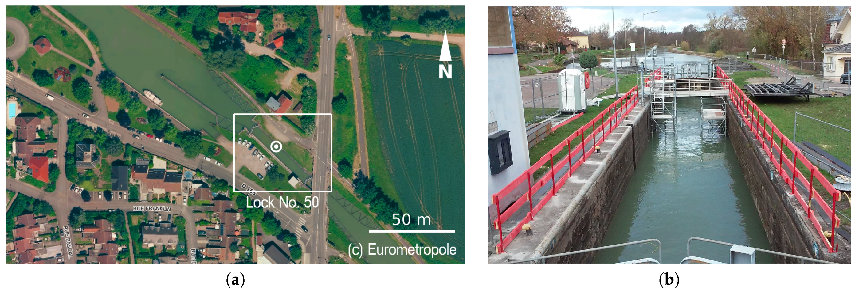
In this section, we describe the site where we performed our experiments, the sonar and laser sensors used, as well as the acquisition configurations implemented.

3.1. Test Site

The experimental site is a lock on the Marne-Rhine Canal, operated by Voies Navigables de France (VNF). Located in the northeast of France, this 313 km long canal was opened in 1853. It connects the Marne river, in Vitry-le-François, with the Rhine, in Strasbourg. The dimensions of its 154 locks are governed by the Freycinet gauge: a minimum 38.5 m long, 5.05 m width and 2.5 m draught. Our test structure, lock No. 50, is located in Souffelweyersheim, in the vicinity of Strasbourg (Figure 1). It has a rise of about 1.6 m and its chamber is indeed a little wider than the gauge: 43.2 m long, 5.2 m wide and more than 2.6 m draught (which corresponds to a sidewall height of 5.1 m). In December 2015, the lock was closed with cofferdams and completely emptied for maintenance operations and a 3D survey whose purpose was to precisely measure its gauge.

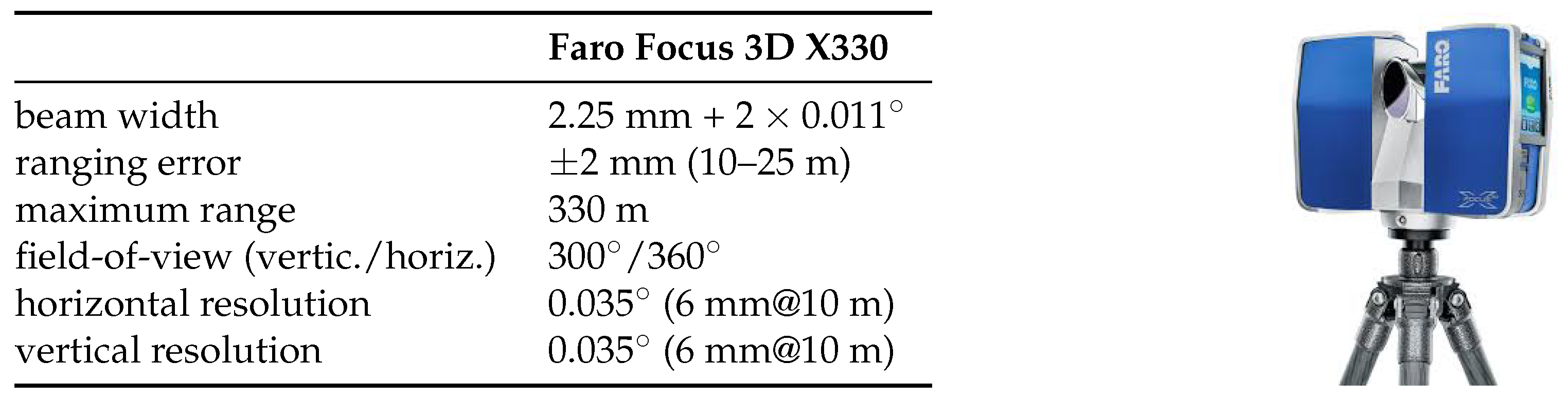
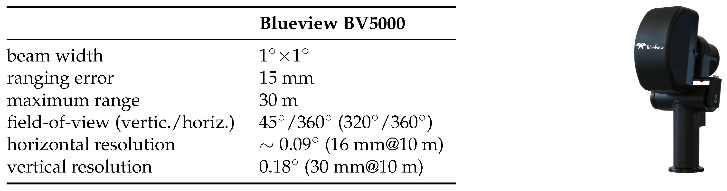
3.2. Description of the Sensors

The empty lock was surveyed using the TLS FARO focus 3D X330 [18]. This device uses phase difference technology to measure the distance between the sensor and the object. As shown in Figure 2, it may be noticed that the field-of-view is an almost complete sphere (360° horizontally and 300° vertically) and the environment may be scanned over a range from 0.6 m to 330 m. Note also that the beam divergence (0.011°) is quite low. All these specifications make it very suitable to build a reference model, of centimetric accuracy.
The mechanical scanning sonar Blueview BV5000 has been used for scanning the water-filled lock. This device consists of a MB1350 multibeam echosounder, mounted on a rotating system that enables scanning the environment through 360°. The specifications of the sonar are provided in Figure 3. The high acquisition frequency of the device (1.35 Mhz, and thus an associated wavelength of 1 mm) allows for estimating the distances with a very high resolution. However, the sonar range is reduced to a maximum of 30 m.
The MBES is mounted on its pan-tilt mechanism so that its swath is vertical. Since the field-of-view of MB1350 is limited to 45°, it is necessary to tilt the sensor at different angles to scan the entire height of the walls. The mechanical scanning system thus allows the sonar to be used in a manner similar to a TLS, providing the user with 3D “laser-like” measurement capabilities underwater, as argued by the manufacturer. However, compared to TLS specifications, it may be observed significant differences in terms of beam divergence (1° for MSS vs. 0.011° for TLS). As noticed in [4], this results in a lower spatial resolution for the MSS, in particular for points of the surface that are located at a high distance from the scanning location.
This is illustrated by Table 1, where the footprint sizes of laser and sonar signals on a vertical surface (such as lock chamber walls) are given. The configuration taken into account for the calculation of these sizes is typical of surveying applications in confined environments, where the sensor is located at a short distance from the imaged surfaces, which causes grazing incidence angles. More specifically, the 2.6 m distance corresponds to the center of the lock chamber. The laser footprint on the surface is an ellipse, while the sonar print is almost rectangular. As can be seen, the sonar footprint size varies much faster than that of the laser.

3.3. Data Acquisition

The TLS survey was carried out by the Photogrammetry and Geomatics Group (INSA Strasbourg) on 1 December (some complementary scans were taken on the next day, after scaffolding disassembly). A total of six scans were taken from the bottom of the empty lock, and eight from the top, using the Faro Focus 3D X330. Both configurations are illustrated in Figure 4. We used spherical targets (as the one that is visible in Figure 5), distributed around the structure, to facilitate the registration of the point clouds. The coordinates of the sphere centres were established using traditional survey methods based on a set of reference points implemented on the site in a local coordinate system. A sample model of the top structure of the lock is shown in Figure 5b. It can be noticed that, since there was a little bit of water left at the bottom of the lock chamber, the latter could not be modelled.
The MSS survey was carried out by a subcontractor, the sub-C Marine company, on 4 December, immediately after the lock was refilled. The lock chamber was therefore in almost the same condition as for the TLS survey: the only notable difference is that the bottom door was open for the TLS survey and closed for the MSS survey. The water in the canal is rather turbid, as the images in Figure 4 and Figure 5 show. The speed of sound in this medium, which is a necessary parameter for any sonar measurement, was about 1434 m . s 1 (measured with SonTek’s CastAway-CTD sensor, SonTek, San Diego, CA, USA).
The MSS was deployed in two different ways. In the first configuration, it was placed on a tripod and deposited at the bottom of the lock using ropes (see Figure 4c). We have made three acquisitions in this configuration, which is similar to that of the TLS, as we have already pointed out. The problem of localizing the scans is, however, more difficult than in the case of TLS because the MSS is not visible from the surface. Although there exist spherical targets to consolidate MSS data, in the same spirit as for the TLS (with the difference that they are open to better adapting to the sonar signal, see [3]), we have not used any here. Instead, we implemented a second configuration, illustrated in Figure 4d and Figure 5c, in which the MSS is immersed in water upside down. To do this, a ladder is placed through the lock. In the middle of it, a metal mast, at the end of which the MSS has been fixed, plunges into the water. In this way, the MSS is located approximately 80 cm below the surface. A topographic prism is attached to the fixation of the pole on the ladder. The prism and a couple of target points on the axis of the pole were carefully surveyed with a total station. Using this information, it is possible to roughly register each scan. More specifically, the three translations and two angles out of three may be estimated straightforwardly. Details on the calculation are given in Section 4.3, where we also propose a method for recovering the remaining third (horizontal) rotation angle.
With this “head down” implementation, acquisitions were made every 5 m along the lock, thus providing nine point clouds in total. At each scanning position, the sonar head made three 360° rotations around its vertical axis, with a 15°, −15° and −45° tilt. In this configuration, the maximum angle of incidence is 75° and the maximum sight distance is five meters. Figure 6 illustrates the variations in acquisition distances and incidence angles on the right sidewall of the lock chamber. One can notice that, by plunging the sonar more deeply, both quantities would decrease, leading to more favorable scanning geometries. Figure 5d shows a crude model of the top structure of the lock, obtained after a manual registration of several raw MSS scans (taken in different MSS configurations).

4. Construction of the 3D Models

In this section, we describe how the 3D models used for the evaluation are constructed. While laser data registration is easy, sonar data processing requires more steps. Their noisy nature and the artefacts observed require a special pre-processing. In addition, we had to correct the tilt angle, initially miscalibrated on the device used. Finally, the alignment and registration of the data required the development of a specially adapted method.

4.1. Laser Data Processing

The registration of laser data in a local reference frame was carried out using classical techniques [18], using spheres of known position. This was done within the Faro ® Scene framework. We observed a sub-centimeter accuracy between the positions of sphere centers measured by conventional tacheometric methods and those measured in the laser scans. As already noticed, the bottom of the lock chamber is not modelled since it could not be accurately surveyed due to the residual water film. The resulting model, shown in Figure 7, will be considered as a reference for the rest of the study. Note that this model was also used by VNF to establish the precise gauge of the lock.

4.2. Sonar Data Pre-Processing

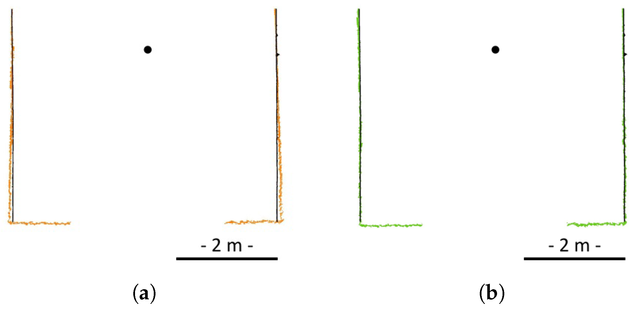
4.2.1. Review of the Observed Artefacts

As can be observed in Figure 5, the information provided by the TLS and the MSS are noticeably different. The most notable visual difference is the granular appearance of the sonar model. This is also visible in Figure 8, which presents the raw data produced by the MSS without any post-processing. Beyond the noisy aspect of the scan, five types of artifacts can be noticed in that figure. In the following, we propose to interpret them, in light of considerations about the employed technology, the experimental setup and the characteristics of the surveyed object.
First, several artifacts are due to signal reflections on the water surface. These points are colored in salmon in Figure 8, detail No. 1. They can easily be removed if the water level is known. The latter is difficult to estimate accurately using the point cloud alone, especially in our case, since sidewalls are flat and smooth. This is why it is preferable to use external measurements. For example, in [4], we used ladders to recover this information. In the present study, the water level was measured with a tacheometer. The reflection phenomenon is also observed for other surfaces (typically the walls). The corresponding points are removed manually, as the shape of the lock is approximately known, making these aberrations easily detectable. Other artifacts are attributed to acoustic phenomena occurring in water. This results in “ghost” objects (see No. 2 in Figure 8) or in systematic patterns occurring when the signal is backscattered by a surface (No. 3 in Figure 8). In our study, all these outliers were manually removed from each point cloud before registration.
Next, the granular aspect of the data becomes more and more visible as the distance from the acquisition position increases. This is also noticeable in the horizontal cross section shown in Figure 9. These increasing inaccuracies may be explained by the noise inherent in sonar measurement. They are also related to the increase in signal footprint size with distance, since the narrowness of the canal yields more and more unfavorable incident angles (Section 3.2). To reduce noise, specific filtering algorithms must be used. In [4], we proposed a method that combines denoising and meshing. It enables a visual control on the result and is well suited to simple environments, such as walls. In the present paper, this technique was used for visualizing details (Section 5.2). However, the sonar model evaluated in section Section 5.1 was not denoised.
Some artifacts seem to be related to the mechanical scanning system. For example, it can be seen that some profiles, which correspond to successive acquisition angles, are very similar (see No. 4, Figure 8). A possible explanation is that the rotative mechanism temporarily blocks while the system carries on incrementing the value of the acquisition angle. This error impairs the geometry of the point clouds. For example, the sidewall point cloud in Figure 9 shows anomalous curvatures. This provides an a posteriori justification of our choice of implementing scanning positions every 5 m, which allows for truncating the model before the geometric effects become preeminent.
In addition, the geometry of the point cloud can also be distorted if the tilt angle of the sonar assigned to the data is incorrect [3]. This error is observed when comparing the vertical cross sections of the TLS and MSS data (see Figure 10a): the sidewalls appear to be inclined towards the inside of the lock in the sonar point cloud, whereas they appear vertical in the TLS model. We propose in Section 4.2.2 a method to recalibrate the tilt angle and correct this problem of geometry.
Finally, we noticed on almost all point clouds that some areas are not surveyed (see No. 5 in Figure 8). This lack of data, which is not yet explained, has variable angular size, but it generally occurs at the same horizontal acquisition angle. We note that similar gaps can be observed in many published results, e.g., in Figure 4.9, p. 74 in [19].

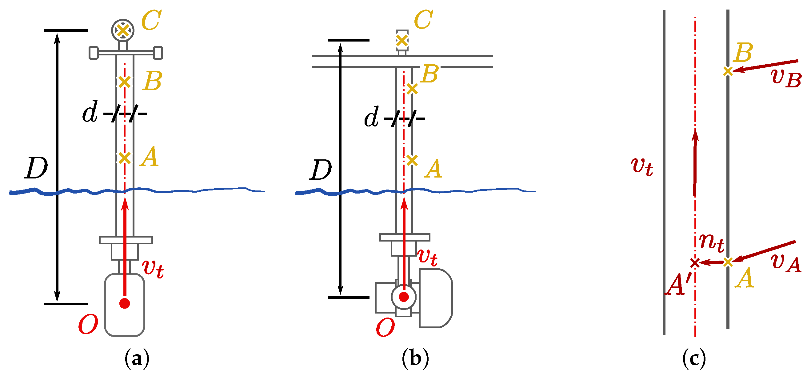
4.2.2. Tilt Angle Correction

The tilt angle is the configurable angle between the sight direction and the 360° rotational axis of the device. The system must accurately achieve the angular setpoint specified by the operator, which requires prior calibration of potential offsets [3]. The geometrical deformations noticed in Figure 10a were related to a defect in the tilt angle calibration of the apparatus we used in our experiments, as we have demonstrated with the help of numerical simulations in [5]. In this section, we propose a method to make an a posteriori correction of the sonar data. This correction in itself is rather simple: it consists of transforming the raw Cartesian coordinates of the sonar point clouds into polar coordinates, applying a previously estimated tilt angle correction (angular offset), and in transforming the coordinates back into Cartesian ones. The origin of the coordinate system is taken at the intersection of the two rotation axes of the pan and tilt unit of the MSS. The main issue is therefore the estimation of the tilt offset. For this, we can take advantage of the existence of laser data describing precisely the surveyed structure.
In the first method tested, we started from the sonar model obtained as is described in Section 4.3. We then sought the correction angle that minimizes the average difference in the distance between the corrected sonar model and the laser reference model (according to a point-to-cloud distance as proposed in Section 5.1). A simulation on TLS data [5] having shown that a value slightly higher than the degree should explain the artefacts observed, we implemented a dichotomic search technique. More specifically, we first tested three angles (−1.318°, −1.375° and −1.432°) and refined the search until the average distance was less than 10 5 m. The resulting offset was −1.324°.
The second method tested is based on the analysis of the inclination of flat areas digitized both by sonar and by the terrestrial laser scanner. Here, a scan taken from the canal bottom (configuration in Figure 4c) is used. Two areas on both sides of the lock were segmented manually in the sonar and laser point clouds. A plane was fitted on each of these point sets thanks to a robust Principal Component Analysis (PCA), as described in [4]. The difference in orientation (in a vertical plane) between the vector normal to the plane of the sonar data and that of the laser data, on each side of the channel, is averaged to obtain the desired angular offset. Note that, while the laser model is level, this is not necessarily the case with the sonar. Potential imperfections (in a vertical plane) have symmetric effects on opposite walls and, thus, they compensate each other when computing the average of the orientation differences. The offset obtained is −1.346°, which corroborates the results of the first method. However, the advantage of the second method is that it does not involve the sonar model that will be used later for quantitative analysis, and that it uses laser data in a rather minimalist way. Figure 10b shows a cross section of the sonar cloud after orientation correction, which illustrates the effectiveness of the technique.

4.3. Alignement and Registration of Sonar Scans

In order to build the entire 3D model of the lock from underwater acquisitions, an original method was deployed. Its aim is to align the scans obtained with the MSS suspended from the surface. The proposed consolidation process consists of two steps: each point cloud is first translated and levelled using topographic measurements; the point clouds are then oriented horizontally.

4.3.1. Leveling and Translation

The purpose of this first step is to determine, for each scan, the translation and rotations to be applied so that the sonar rotation axis is oriented in the local coordinate system, which is what we call leveling. To do this, the two parameters needed are the sonar acquisition center, O, and the rotation around the horizontal axis of the MSS, which corresponds to the direction of the pole that connects the MSS to the ladder, v T . In order to determine these quantities, three positions were measured on the system using traditional topography techniques (total station). These target elements are two points (A and B) on the axis of the tube and a prism placed above it, C. These three points are illustrated in Figure 11.
Points A and B give the orientation of the tube, from which we deduce the unit normal vector n T that points towards the tube axis:
n T = v T ( v A v B ) ,
where v A and v B are the unit vectors defining the viewing direction of points A and B from the total station. Then, the projection A of A on the tube axis is straightforwardly obtained:
A = A + d 2 n T ,
provided the tube diameter, d, is known. From points A and C and distance D = O C measured beforehand, the coordinates of point O are defined as follows:
O = A + ( D v A C · v T ) v T .
Once the coordinates of the sonar acquisition center O and its vertical orientation ( v t ) have been calculated, determining the translations and rotations associated with each scan is simple: all that remains is then to translate and level the acquisitions.

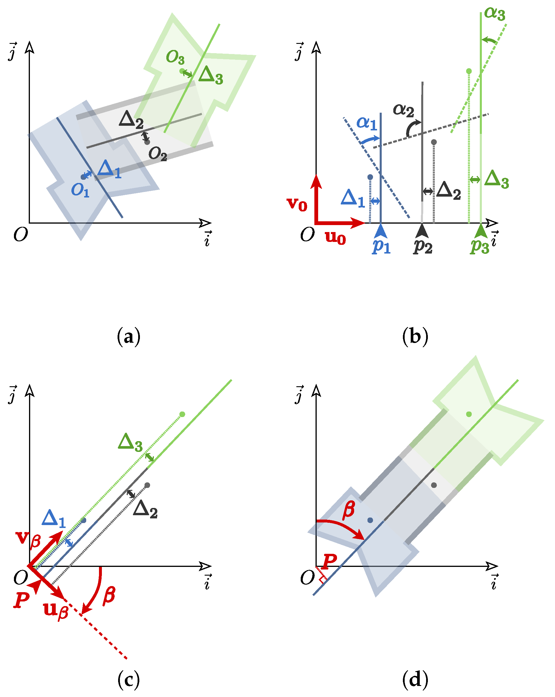
4.3.2. Horizontal Orientation

The second step is to determine (and compensate) the horizontal rotation of the scans. In practice, this means estimating, for each sonar digitization, the rotation around the vertical axis passing through the associated acquisition center O i . The process we propose consists of three steps that are illustrated in Figure 12.
The first operation consists of determining the axis of the canal in each point cloud (see Figure 12a). In our approach, we assume that the lock chamber is symmetrical in a vertical plane, which defines the longitudinal axis of the lock. It is estimated for each MSS cloud using a Principal Component Analysis and selecting the eigenvector corresponding to the maximum eigenvalue. In the rest of the process, we try to align these symmetry axes by applying to each of them a rotation along the vertical axis passing through its sonar acquisition center, O i . In this manner, these locally determined lock axes will be aligned with the global lock axis, which is oriented along an azimuth β and which is at a distance P from the origin of the coordinate system, as shown in Figure 12d. When solving this problem, the sonar acquisition centers O i as well as their distances to their associated symmetry axes ( Δ i ) must remain fixed.
In reality, the rotation sought can be broken down into two rotations. First, each axis is rotated an angle α i , so that its direction is oriented along the ordinate axis (see Figure 12b). At this point, the distances between the origin and each of the axes are obtained as follows:
p i ( 0 ) = u 0 O i + Δ i where u 0 = i .
Moreover, from this configuration, applying an arbitrary β angle rotation to all axes’ amounts to orienting them along an azimuth β . One can calculate the original distances p i as a function of β using the following expression:
p i ( β ) = u β O i + Δ i where u β = R β u 0 with R β = cos β sin β sin β cos β .
If all the axes are aligned, then they are identical with the overall axis of the lock, as Figure 12c shows. In this case, β = β and all p i values are equal to P. In practice, there are always imperfections, so we estimate β and P in the least squares sense by minimizing:
J ( P , β ) = i p i ( β ) P 2 .
By developing this expression, one obtains the following formula:
J ( P , β ) = i x O i cos β y O i sin β + Δ i P 2 with O i = x O i y O i .
Since the objective function is not linear with respect to β , we use the Gauss–Newton optimization method. The approximate solution necessary for its initialization is obtained by aligning the axes of the digitizations carried out at the extremities of the lock chamber.
In this way, we were able to align the axes and thus consolidate the 3D model. Figure 13 presents the resulting global 3D MSS model of the lock, which can be compared to the 3D model generated with the acquisitions of the TLS (Figure 7). The proposed method produces visually satisfactory results. However, improvements may be envisioned. Indeed, the solution found might be refined by using global techniques, such as ICP [16]. In this way, no assumption about the lock geometry would be necessary. However, this method requires overlap between scans, so one would have to consider longer chunks, which is exposed to noise and loss of resolution. Therefore, the estimate should be weighted according to the distance and angle of incidence to lessen their effect.

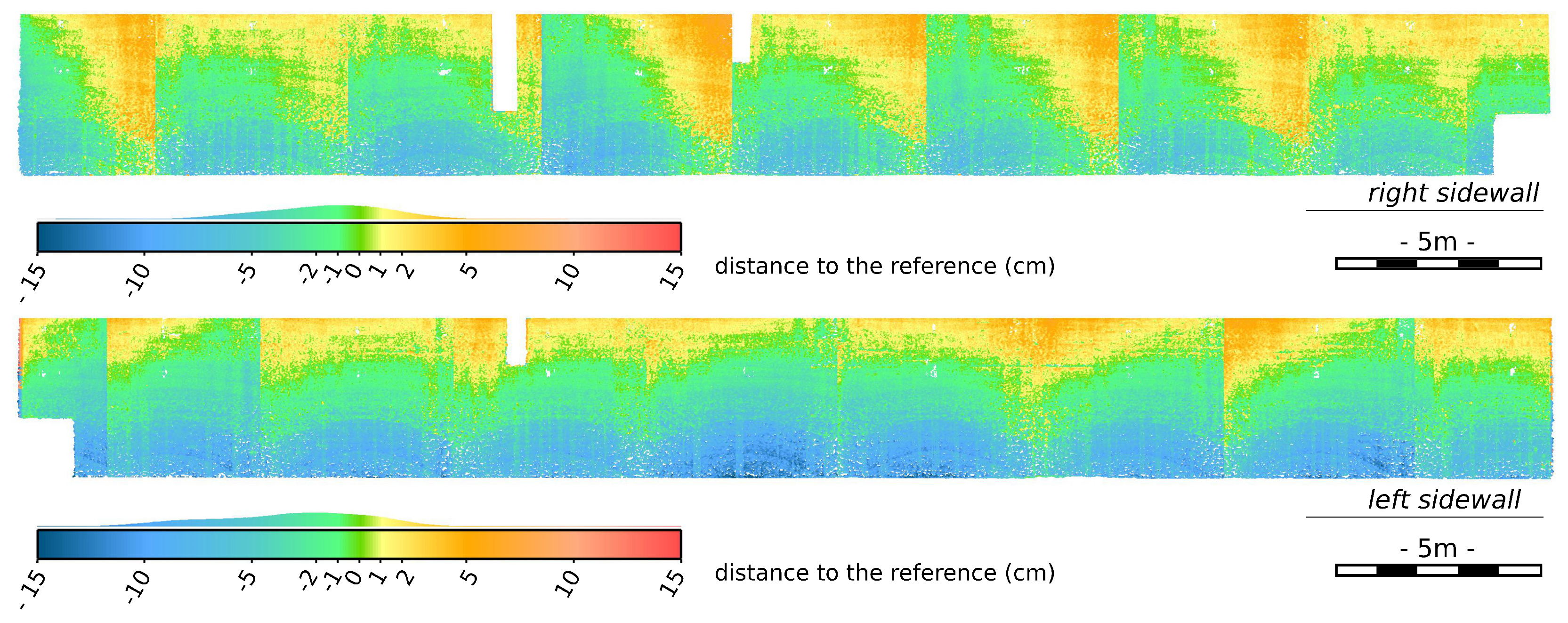
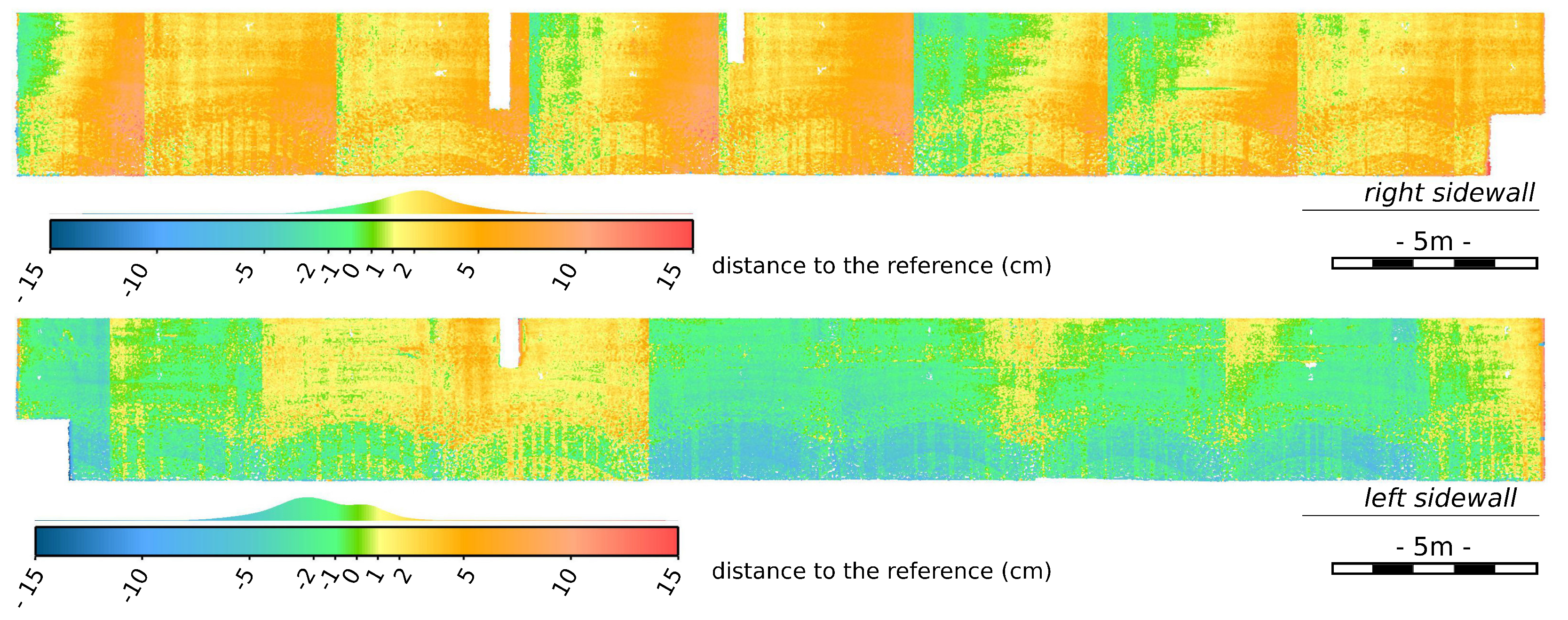
5. Comparison of Sonar and Laser Models

In this section, we study the quality of the 3D sonar model (Figure 13) with respect to the reference laser one (Figure 7), from both a quantitative and a qualitative point of view.

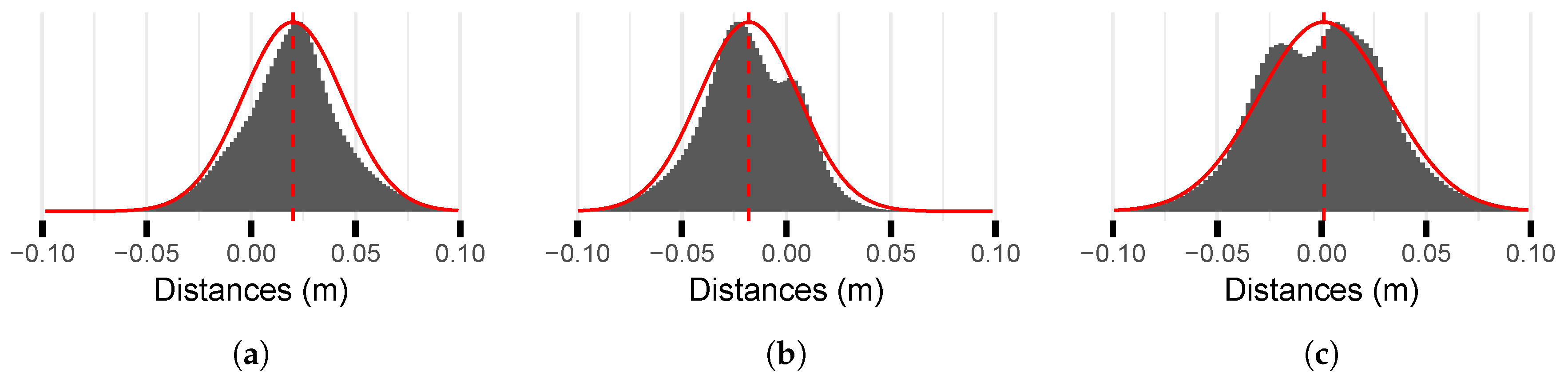
5.1. Quantitative Evaluation

In the first place, we propose a quantitative evaluation of the 3D sonar model of the lock chamber, compared to the laser model, considered as a reference model. The sonar data alignment method presented in Section 4.3 provides a full 3D model, in the same coordinate system as the TLS model. As a result, the assessment can be done directly, without further adjustment. The disadvantage is that the result depends both on the quality of the MSS data and on the efficiency and robustness of the registering method.
In order to facilitate comparisons, the topologies of the compared surfaces must be simple, i.e., they must be relatively smooth and almost without occultation. This is why the models have been segmented to retain only the walls (see Figure 14). Moreover, the result of a cloud-to-cloud comparison depends strongly on the density of the point clouds. To alleviate this problem, one solution is to mesh the reference cloud, which we do with Technodigit’s 3DReshaper ® software (Neyron, France, www.3dreshaper.com). Finally, the cloud-to-mesh comparison is performed with CloudCompare (www.cloudcompare.org), which uses an algorithm inspired from Metro [20]. In practice, since no reference is available for the floor of the lock, the comparison is carried out for each wall separately.
This study was performed before and after correction of the sonar tilt angle. First, a spatial visualization of the distance distributions between the sonar point cloud and the meshed TLS model is proposed in Figure 15 before tilt angle correction, and in Figure 16 after it. While a systematism is apparent in the distance distributions before correction in the form of repetitive patterns, it is attenuated afterwards: the results are more uniform. However, it seems that, in certain scans, after tilt correction, the distances increase at one end. In this case, the error due to a blockage of the rotating system is probably the cause.
The quantitative results of the distance calculation are summarized in Table 2. As can be seen, the tilt angle correction operation reduces the differences between the sonar and laser modeling. The histograms in Figure 17 show that the distance distributions, calculated for the global cloud and for the individual wall clouds, are close to the Gaussian.
The differences between the sonar and laser models are between –9.8 and 10.7 cm. The average (considering both walls simultaneously) of the distances is 0.1 cm and the standard deviation is 3.1 cm. However, when one observes the averages of the deviations for each wall in the table and on the histograms, one notes a bias of approximately 2 cm. This bias represents a slight translation between the TLS and MSS model transversely to the lock axis. This explanation seems to be confirmed when we look at Figure 16. These results might be enhanced by improving the registration method.

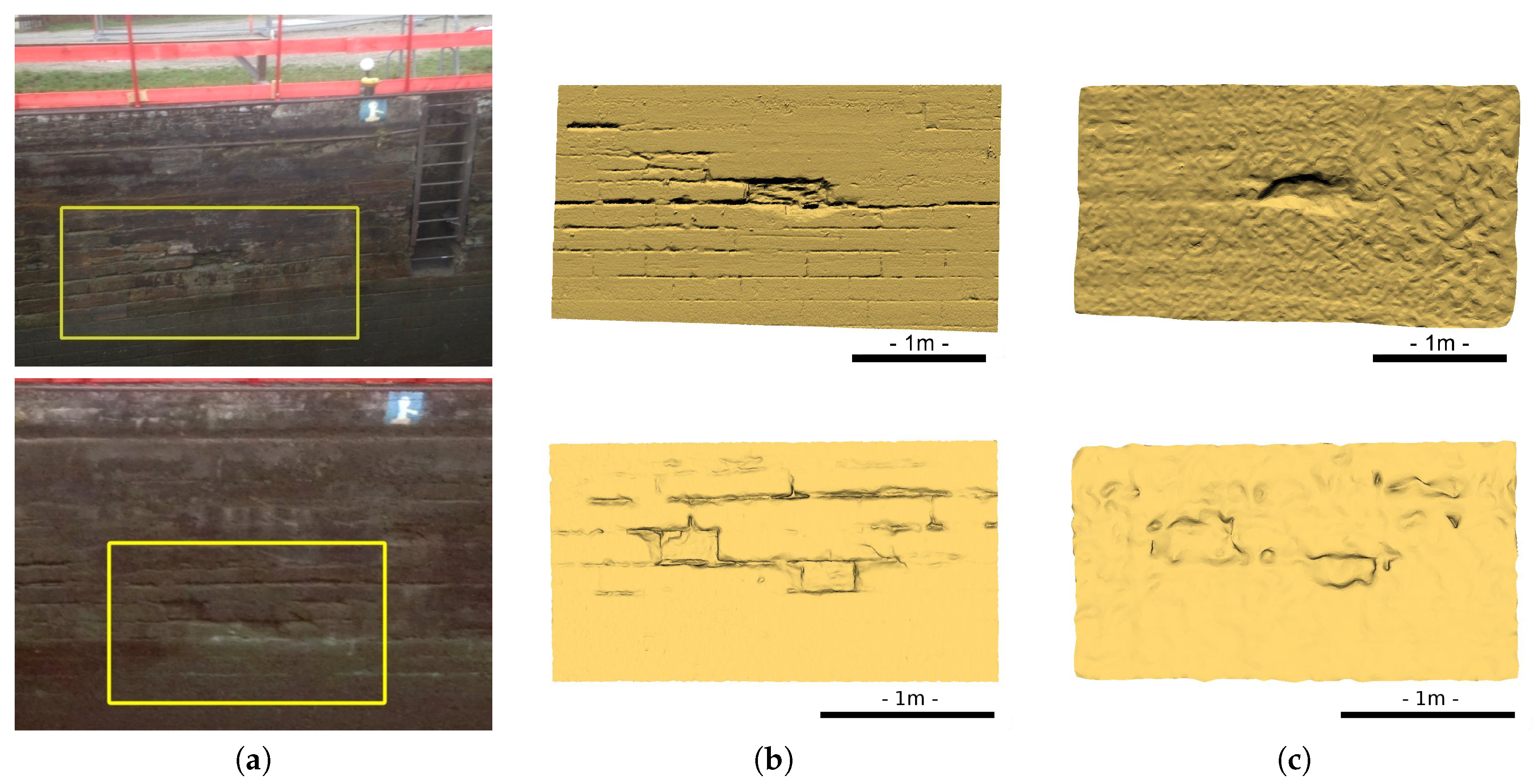
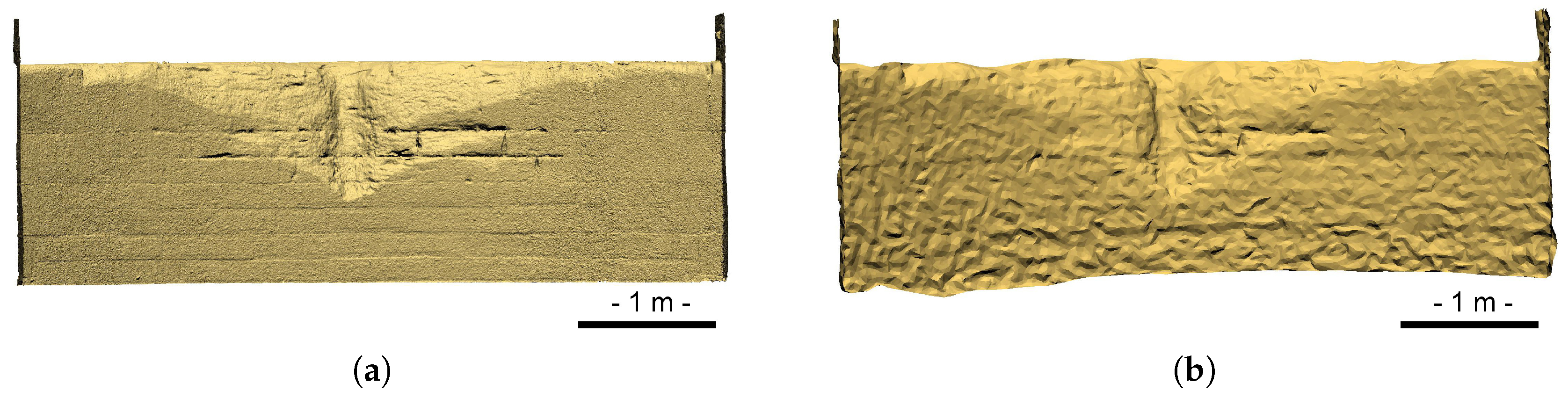
5.2. Qualitative Examination of Details

In this second experimental study, we focus on the ability of the MSS to model distinguishable details of the lock structure. To this aim, we consider three areas of the lock chamber. The first two ones are located on the left wall. In the first area (top line in Figure 18), a rubber stone (approximate dimensions: 60 × 20 × 10 cm) is missing and masonry joints are damaged (these crevices are about 4 cm wide and 4 cm deep). To make visualization easier, the sonar model is a meshed extract from an acquisition made with the suspended MSS. The defects are easily visible in the laser model, Figure 18b, while only the missing block may be detected in the sonar model, Figure 18c. The appearance of the sonar model, rougher on its right part than on its left part, is related to the variation of the dimensions of the sonar beam footprint with respect to the angle of incidence and the distance, and thus with respect to the resulting change in spatial resolution. The sonar model is of a better quality in the second example (bottom line in Figure 18), but the visual results are of the same kind as for the first example.
The third area is the lock threshold wall, which was acquired with the MSS placed on a tripod on the chamber floor, about 5 m from the target. The sonar placement was similar to that of the TLS when surveying the empty lock. A spall in the threshold wall creates a cavity whose dimensions are about 50 × 100 × 15 cm. Damaged joints are also visible in this area. A meshing of this particular MSS model is also performed (see Figure 19).
These examples visually demonstrate that defects of a significant size in the masonry, such as missing rubble or cavities, are detected in the point cloud acquired by the MSS. However, details below 4 cm, such as damaged masonry joints, are more difficult to detect. This evaluation validates the relevance of using an MBES for this type of measurement, and allows a better understanding of the smallest size of accessible defects. Finally, we note that the quality of detail restitution of the MSS varies according to the distance and the angle of incidence of the acquisitions. This militates for the use of close acquisition positions, even if it means using the MBES with an orthogonal incidence to the studied surface (which is the case when it is employed for dynamic acquisitions).

6. Conclusions

In this paper, we have reported on the experimental assessment of a Mechanical Scanning Sonar, the BV5000, for 3D surveying in a canal lock. The proposed scanning methodology is based on several acquisitions from the surface, which allows a rough positioning of the scans. We introduced a geometric method for estimating the last missing angle and then registering the scans to obtain a 3D model of the lock chamber. We proposed a qualitative and quantitative assessment of the resulting 3D underwater point cloud, using a meshed model derived from TLS scans as a reference. This study allowed us to quantify the overall precision and level of detail that are accessible with this kind of technique. In particular, while the measuring performance of MSS is rather coarse, they can be appropriate for detecting defects of a decimetric size.
Our study also shed light on the fact that specific external information, such as the water level, the MSS positions or the symmetry of the structure, which could be considered as restrictive factors, can be valuable to remove artefacts, register scans or correct calibration errors.
Furthermore, several optimizations could lead to improved performance. Firstly, to access a better level of detail, noise should be suppressed and precision should be enhanced. To this aim, modifications of the setup may be envisioned. For example, reducing the inter-scan distances and immersing the MSS a little deeper would lead to more favorable sight distances and incidence angles. This would result in smaller footprint sizes and hence a better resolution. In addition, the noise level could be lowered by applying suitable sonar data denoising methods when processing the MSS raw outputs. Secondly, the quality of the global 3D model could be improved. For example, a more precise calibration of the MSS-mast-prism system should improve the measurement accuracy. Moreover, the estimation of registration parameters of the scans might be refined using an iterative procedure. To this aim, a constrained version of the ICP algorithm is envisioned. Finally, a better precision and accuracy can be expected with new generations of Mechanical Scanning Sonars.

Author Contributions

All authors conceived and designed the experiments and performed the acquisitions; the first three authors contributed analysis tools; the first four authors analyzed the data and wrote the paper.

Funding

This work was funded by the Cerema under PhD Grant No. 2014/0002CD.

Acknowledgments

The MSS acquisitions were subcontracted to the Sub-C Marine company (Feyzin, France: www.subcmarine.com). The authors thank them for their availability and their cooperation. Many thanks also to VNF colleagues for their support.

Conflicts of Interest

The authors declare no conflict of interest.

References

  1. Rondeau, M.; Leblanc, E.; Garant, L. Dam infrastructure first inspection supported by an integrated multibeam echosounder (MBES)/LiDAR system. In Proceedings of the CDA Annual Conference, Saskatoon, SK, Canada, 16 October 2012. [Google Scholar]
  2. Rondeau, M.; Stoeffler, C.; Brodie, D.; Holland, M. Deformation analysis of harbour and dam infrastructure using marine GIS. In U.S. Hydro 2015; The Hydrographic Society of America: National Harbor, MD, USA, 2015. [Google Scholar]
  3. Lesnikowski, N.; Rush, B. Spool Piece Metrology Applications Utilizing BV5000 3D Scanning Sonar: High Resolution Acoustic Technology for Underwater Measurement; Technical Report; BlueView Technologies: Seattle, AC, USA, 2012. [Google Scholar]
  4. Moisan, E.; Charbonnier, P.; Foucher, P.; Grussenmeyer, P.; Guillemin, S.; Koehl, M. Adjustment of Sonar and Laser Acquisition Data for Building the 3D Reference Model of a Canal Tunnel. Special Issue Sensors and Techniques for 3D Object Modeling in Underwater Environments. Sensors 2015, 15, 31180–31204. [Google Scholar] [CrossRef] [PubMed]
  5. Moisan, E.; Charbonnier, P.; Foucher, P.; Grussenmeyer, P.; Guillemin, S.; Samat, O.; Pagès, C. Assessment of a static multibeam sonar scanner for 3D surveying in confined subaquatic environments. Int. Arch. Photogramm. Remote Sens. Spat. Inf. Sci. 2016, 41, 541–548. [Google Scholar] [CrossRef]
  6. Ridao, P.; Carreras, M.; Ribas, D.; Garcia, R. Visual inspection of hydroelectric dams using an autonomous underwater vehicle. J. Field Robot. 2010, 27, 759–778. [Google Scholar] [CrossRef] [Green Version]
  7. Paull, L.; Saeedi, S.; Seto, M.; Li, H. AUV Navigation and Localization: A Review. IEEE J. Ocean. Eng. 2014, 39, 131–149. [Google Scholar] [CrossRef]
  8. Massot-Campos, M.; Oliver-Codina, G. Optical Sensors and Methods for Underwater 3D Reconstruction. Sensors 2015, 15, 31525–31557. [Google Scholar] [CrossRef] [PubMed] [Green Version]
  9. Mallios, A.; Ridao, P.; Ribas, D.; Hernández, E. Scan matching SLAM in underwater environments. Auton. Robots 2014, 36, 181–198. [Google Scholar] [CrossRef]
  10. Henderson, J.C.; Abbott, B. Using Sector-Scan Sonar for the Survey and Management of Submerged Archaeological Sites. Int. J. Naut.l Archaeol. 2016, 46, 330–345. [Google Scholar] [CrossRef]
  11. Drap, P.; Merad, D.; Boï, J.M.; Boubguira, W.; Mahiddine, A.; Chemisky, B.; Seguin, E.; Alcala, F.; Bianchimani, O. ROV-3D: 3D Underwater Survey Combining Optical and Acoustic Sensor. In Proceedings of the 12th International Conference on Virtual Reality, Archaeology and Cultural Heritage, Aire-la-Ville, Switzerland, 18–21 October 2011; pp. 177–184. [Google Scholar]
  12. Drap, P.; Merad, D.; Boï, J.M.; Mahiddine, A.; Peloso, D.; Chemisky, B.; Seguin, E.; Alcala, F.; Bianchimani, O. Underwater Multimodal Survey: Merging Optical and Acoustic Data. In Underwater Seascapes: From Geographical to Ecological Perspectives; Musard, O., Le Dû-Blayo, L., Francour, P., Beurier, J.P., Feunteun, E., Talassinos, L., Eds.; Springer International Publishing: Cham, Switzerland, 2014; pp. 221–238. [Google Scholar] [Green Version]
  13. Sohnlein, G.; Rush, S.; Thompson, L. Using manned submersibles to create 3D sonar scans of shipwrecks. In Proceedings of the IEEE OCEANS Conference, Waikoloa, HI, USA, 19–22 September 2011; pp. 1–10. [Google Scholar]
  14. Kaufmann, K.E. Using Divers and 3D Sonar Technology to Study Historic Shipwrecks in Lake Michigan. In Diving For Science 2015: Proceedings of the AAUS 34th Scientific Symposium, Key West, FL, USA, 28 September–3 October 2015; Lobel, L., Ed.; AAUS: Dauphin Island, AL, USA, 2015; pp. 40–47. [Google Scholar]
  15. Thompson, R.L. New 3D Acoustic Scanning Tools and Techniques for Underwater Metrology and Inspection. OTC-21940-MS. In Proceedings of the Offshore Technology Conference, Houston, TX, USA, 2–5 May 2011. [Google Scholar]
  16. Besl, P.; McKay, N. A method for registration of 3-D shapes. IEEE Trans. Pattern Anal. Mach. Intell. 1992, 14, 239–256. [Google Scholar] [CrossRef]
  17. Chen, Y.; Medioni, G. Object modeling by registration of multiple range images. Image Vis. Comput. 1992, 10, 145–155. [Google Scholar] [CrossRef]
  18. Grussenmeyer, P.; Landes, T.; Doneus, M.; Lerma, J.L. Basics of range-based modelling techniques in Cultural Heritage 3D recording, chapter 6. In 3D Recording, Documentation and Management in Cultural Heritage; Remondino, F., Stylianidis, S., Eds.; Whittles Publishing: Dunbeath, UK, 2016; pp. 305–368. [Google Scholar]
  19. Thomas, L. The A.J. Goddard: Reconstruction and Material Culture of a Klondike Gold Rush Sternwheeler. Master’s Thesis, Texas A&M University, College Station, TX, USA, 2011. [Google Scholar]
  20. Cignoni, P.; Rocchini, C.; Scopigno, R. Metro: Measuring Error on Simplified Surfaces. Comput. Graph. Forum 1998, 17, 167–174. [Google Scholar] [CrossRef]
Figure 1. Presentation of Lock No. 50 on the Marne-Rhine canal. (a) aerial view (WGS84 coordinates of the white circled dot: 48.6338° N, 7.7537° E); (b) view of the lock during emptying operations.
Remotesensing 10 01395 g001
Figure 2. Characteristics and photograph of the Faro ® Focus 3D X330 TLS.
Remotesensing 10 01395 g002
Figure 3. Characteristics and photograph of the Blueview ® BV5000 MSS.
Remotesensing 10 01395 g003
Figure 4. Schematic view (top line) and photograph (bottom line) of the configurations used for the survey: TLS from (a) the top and (b) the bottom of the lock chamber; MSS operated (c) using an immersed tripod or (d) upside down from the water surface. TLS acquisition items appear in red, MSS items in blue, and tacheometric ones in yellow.
Remotesensing 10 01395 g004
Figure 5. Sample 3D models of the top structure of the lock: (a) extremity of the empty lock (near the top gate); (b) corresponding TLS model; (c) view of the ladder supporting the fixation of the MSS (pole) and a tacheometric prism (the tacheometer is visible in the background); (d) MSS model (manually processed).
Remotesensing 10 01395 g005
Figure 6. (top) TLS mesh of the right sidewall of the lock chamber (reference): the two indentations correspond to a ladder and to a groove used for the lock paddle commands, the threshold is visible on the right; (middle) incidence angles; (bottom) sight distances.
Remotesensing 10 01395 g006
Figure 7. 3D laser model of the lock.
Remotesensing 10 01395 g007
Figure 8. Rendering of a raw sonar output (from a single scanning position on the lock chamber floor). 1: artifacts due to surface reflections (coloured in salmon). 2: acoustic anomalies in the water column. 3: acoustic phenomena due to signal backscattering. 4: acquisition anomaly probably due to a temporary blocking of the horizontal rotation system. 5: lack of measurement.
Remotesensing 10 01395 g008
Figure 9. Horizontal cross section of the MSS (blue) and TLS (green) point clouds, where the sonar head position is marked by a black dot. The alignment of the models is done by the method described in Section 4.3.
Remotesensing 10 01395 g009
Figure 10. Vertical cross section of the MSS (in color) and TLS (in black) point clouds: (a) before and (b) after tilt angle correction.
Remotesensing 10 01395 g010
Figure 11. View of the acquisition system with the MSS suspended, (a) in the viewing direction of the total station and (b) perpendicular to that direction; (c) enlarged view of the tube.
Remotesensing 10 01395 g011
Figure 12. Illustration of the horizontal alignment procedure for sonar scans. (a) determination of the longitudinal axis for each digitization using PCA; (b) alignment of the axis of each digitization along the ordinate axis; (c) estimation of the second rotation to be applied to align the axes; (d) application of both rotations to each scan.
Remotesensing 10 01395 g012
Figure 13. Complete 3D sonar model of the lock. The nine scans are represented with different colors.
Remotesensing 10 01395 g013
Figure 14. (top) Evaluated sonar point cloud and (bottom) laser reference mesh.
Remotesensing 10 01395 g014
Figure 15. Distribution of distances between the sonar point cloud and the mesh constructed from TLS data, before tilt angle correction (top) for the right wall and (bottom) for the left wall.
Remotesensing 10 01395 g015
Figure 16. Distribution of distances between MSS and TLS after tilt angle correction, (top) for the right wall and (bottom) for the left wall.
Remotesensing 10 01395 g016
Figure 17. Statistical distributions of the distance between the laser mesh and the sonar point cloud for (a) the right and (b) left lock walls, as well as (c) for the total of the two walls. The Gaussian models fitted to these distributions are represented by the red curves.
Remotesensing 10 01395 g017
Figure 18. Details on two areas of the left lock wall: (a) localization; (b) laser model; (c) sonar model.
Remotesensing 10 01395 g018
Figure 19. Front view of the (a) laser and (b) sonar models of the threshold wall. Both TLS and MSS scans were taken from the bottom of the lock.
Remotesensing 10 01395 g019
Table 1. Horizontal size of the sonar/laser footprint on a vertical wall located 2.6 m in front of the sensor vs. the horizontal position of the measured point on the wall, i.e., its distance to the orthogonal projection of the sensor on the wall.
Position on Wall (m)012345678910
Sonar footprint (cm)4.545.217.2210.5815.2821.3328.7237.4547.5458.9771.75
Laser footprint (cm)0.320.360.440.580.750.961.201.471.772.112.47
Table 2. Analysis of the distributions of distances between the laser mesh and the sonar point cloud before and after tilt correction of the MSS. By convention, the distances are positive when the sonar points are inside the lock in the laser model (i.e., the points from the MSS are closer to the center of the lock than their counterparts from the TLS). Distances are given in centimeters.
Right WallLeft WallOverall
OriginalRectifiedOriginalRectifiedOriginalRectified
Mean−1,62,0−3,3−1,8−2,40,1
Standard dev.3,02,43,72,43,53,1
Max6,510,77,710,3−14,410,7
Min−10,6−6,5−14,4−9,87,7−9,8

