Mapping Population Distribution from High Resolution Remotely Sensed Imagery in a Data Poor Setting


1
Department of Geography, Cartography and GIS Research Group, Physical Geography, Vrije Universiteit Brussel, Pleinlaan 2, 1050 Brussels, Belgium
2
Department of Geography, Physical Geography, Vrije Universiteit Brussel, Pleinlaan 2, 1050 Brussels, Belgium
3
Centre National de Documentation et de Recherche Scientifique, Observatoire Volcanologique du Karthala, 169 Moroni, Comoros
4
Department of Geography, Cartography and GIS Research Group, Vrije Universiteit Brussel, Pleinlaan 2, 1050 Brussels, Belgium
*
Author to whom correspondence should be addressed.
Remote Sens. 2018, 10(9), 1409; https://0-doi-org.brum.beds.ac.uk/10.3390/rs10091409
Submission received: 13 August 2018
/
Revised: 2 September 2018
/
Accepted: 3 September 2018
/
Published: 5 September 2018
(This article belongs to the Section Remote Sensing Image Processing)
Abstract
:Accurate mapping of population distribution is essential for policy-making, urban planning, administration, and risk management in hazardous areas. In some countries, however, population data is not collected on a regular basis and is rarely available at a high spatial resolution. In this study, we proposed an approach to estimate the absolute number of inhabitants at the neighborhood level, combining data obtained through field work with high resolution remote sensing. The approach was tested on Ngazidja Island (Union of the Comoros). A detailed survey of neighborhoods at the level of individual dwellings, showed that the average number of inhabitants per dwelling was significantly different between buildings characterized by a different roof type. Firstly, high spatial resolution remotely sensed imagery was used to define the location of individual buildings, and second to determine the roof type for each building, using an object-based classification approach. Knowing the location of individual houses and their roof type, the number of inhabitants was estimated at the neighborhood level using the data on house occupancy of the field survey. To correct for misclassification bias in roof type discrimination, an inverse calibration approach was applied. To assess the impact of variations in average dwelling occupancy between neighborhoods on model outcome, a measure of the degree of confidence of population estimates was calculated. Validation using the leave-one-out approach showed low model bias, and a relative error at the neighborhood level of 17%. With the increasing availability of high resolution remotely sensed data, population estimation methods combining data from field surveys with remote sensing, as proposed in this study, hold great promise for systematic mapping of population distribution in areas where reliable census data are not available on a regular basis.

1. Introduction
Obtaining reliable estimates of population numbers is important for policy-making, urban planning, and administration, both at the regional and local scale; and it is also fundamental for risk assessment related to natural and human-induced hazards, e.g., References [1,2,3]. According to the United Nations (2015), a count of the population—or ‘census’—must be based on individuals, must be exhaustive and done simultaneously for a given territory, and should be organized at regular intervals, at least every 10 years. The major drawbacks of a census are that it is a complex exercise, which is time-consuming, labor intensive, and expensive [4,5]. To overcome the drawbacks of a traditional census, several countries are nowadays combining different administrative registers to obtain a count of the population and its characteristics (e.g., Belgium, Iceland, The Netherlands) [6]. In data-poor regions though, automating the counting process is not possible due to a lack of up-to-date national civil registers. Therefore, organization of traditional censuses is still required.
If no recent census data are available, the use of remote sensing may be a cost-effective alternative for estimating population numbers e.g., References [7,8,9,10,11,12,13,14,15,16], as it allows large-coverage mapping of human settlements at increasingly higher spatial resolutions. Satellite imagery also makes it possible to provide regular mapping updates for the same area. While estimation of the population from remotely sensed data is not expected to produce results as accurate as a traditional census, it can be a useful approach for producing population estimates between two census dates or in the absence of census data.
In applications of population estimation, remotely sensed imagery may be used in two different ways: (a) To disaggregate census data to a finer spatial scale, using areal interpolation methods; or (b) To define a relationship between remote sensing derived variables and population numbers, using a statistical modelling approach [14]. In the last category of methods, earlier studies have shown that population can be estimated from remote-sensing derived information, such as the number of dwelling units, the area of urban land, the area occupied by different land uses, or even directly from spectral and textural information, available at the pixel scale. Multiplying the number of dwellings in a study area obtained through visual interpretation of aerial photography or high resolution satellite imagery, by the average number of occupants per dwelling obtained through a field survey is considered as time consuming, but it is one of the most accurate ways for population estimation using remotely sensed data [9,11,15,17]. Automated extraction of building outlines from high-resolution imagery using object-based image analysis (OBIA), may substantially lower the cost of data processing, yet the effectiveness of OBIA for successfully identifying individual dwellings strongly depends on spectral/spatial characteristics of the imagery used, as well as the morphological characteristics of the built-up area (i.e., spacing between buildings, sufficient spectral contrast between buildings and their surroundings) [17,18]. If high-resolution LIDAR data or stereoscopic image acquisitions are available, Digital Surface Models (DSM) of the built-up area can be produced. In this case, elevation differences can be used to improve the detection of individual building structures, extract footprint and volume for each building, and calculate available floor space [3,4,19]. Alternatively, in some studies, the number of floors is estimated through building shadow analysis, and in combination with roof area, is used to obtain an estimate of the total floor space per building [20,21]. If no high-resolution data is available, population may be estimated based on the total built-up area, or based on the area covered by different land-use classes, or morphologically homogeneous zones extracted from medium-resolution satellite imagery, using simple regression approaches [10,12,13,16]. Some authors have also explored the potential of directly using spectral and textural responses at the pixel level, to develop regression models to estimate population [7,8,9]. At even coarser scales, imagery showing urban extent has been combined with night-time light emissions, to assess population distribution at continental to global scales [14,19,22,23]. When estimating population from remotely sensed data, numerous physical and socioeconomic variables, obtained from ancillary data sources, can be incorporated as well (e.g., distance to the Central Business District, accessibility to the transport system, slope, period when urban area has been built) [7,24]. By including more variables, the complexity of the model will increase, but the accuracy and the robustness of the model are likely to improve.
In recent years, several studies have focused on estimating population in data-poor regions using high resolution remotely sensed imagery. Population estimation in these studies is mostly based on identifying the number of dwellings, or on estimating the total rooftop area [20,25,26]. Estimates of population are then obtained (a) by multiplying the number of dwellings with an estimated number of people per building structure [25,27], or (b) by multiplying the rooftop area of all buildings with the average number of people per square meter [20,25,26]. Spatial resolution of the imagery in relation to object size, is an important factor for successful extraction of individual dwellings. In informal settlements, where building size may be well below 100 m2, an image resolution of 0.5 m will not be enough [28], and image resolutions of at least 0.3 m will be required to capture small building structures [18]. While OBIA may provide good results for roof top delineation of individual dwellings in well-structured, low to medium dense urban areas [29,30,31], identifying individual dwellings in high-density urban areas, in informal settlements, or in environments where roof type materials show strong spectral similarity with their surroundings remains problematic, and manual digitizing is often the only option left to obtain reliable dwelling counts for population estimation [26,31,32,33]. With the rise of volunteered geographic information initiatives (e.g., www.openstreetmap.org), accurate data on spatial features (e.g., buildings, roads…) is rapidly becoming available for many parts of the world, including developing countries [17]. Therefore, using information on dwelling location, obtained from such data layers, in combination with information on dwelling characteristics captured through remote sensing is a promising avenue for population estimation. The most obvious dwelling characteristic that can be identified from high-resolution imagery is roof type, which in developing countries is often linked to type of housing, household demographics, socio-economic status, and health conditions [34,35,36]. Assuming that household size significantly differs between houses with different roof types, roof type discrimination may be very useful in estimating population numbers, based on available data about the location of individual dwellings.
In this study, we propose an approach to estimate population numbers at neighborhood level, combining information on dwelling location and roof type, obtained from remotely sensed data, with data on household size collected through fieldwork. Given spectral confusion between roof construction materials and the surrounding environment, the complexity of the residential structure, and the absence of ancillary data sources, dwelling locations in our study were obtained by pin-pointing building locations on high-resolution imagery (Pléiades), whilst roof type was extracted from the imagery, using object-based random forest classification. An inverse calibration approach was applied to correct for misclassification bias in population estimation. Uncertainty in model outcome, caused by variations in average dwelling occupancy between neighborhoods was assessed as well. The proposed method was applied on Ngazidja Island (Union of the Comoros). In this data-poor region, no census has been organized since 2003, and there is a need for up-to-date information about population distribution on the island. Model calibration in our study was based on a sample of neighborhoods, for which populations numbers were collected in the field. To assess the accuracy of model outcome, a cross-validation approach was applied using the leave-on-out method. While for this case study, individual dwellings on the island were identified by manually pinpointing dwelling locations on the imagery, with the increased availability of volunteered geographic information datasets, the method proposed might be useful in other areas where such data are readily available, with less cost and effort for data collection.
2. Materials and Methods
2.1. Study Area
The method proposed in this study was applied on Ngazidja Island (Union of the Comoros) (Figure 1). Located northwest of Madagascar, in the Mozambique Channel, Ngazidja is the westernmost island of the Comoros archipelago, and is prone to volcanic hazards. Karthala volcano is the site of recent volcanic activities on the island. In the future, the risk of population and infrastructure being affected by the next eruption is high, because urban areas are surrounding Karthala volcano (Figure 1). Owing to limited budgets and more urgent priorities, the last census in the Union of the Comoros dates back to 2003. There is hence a strong need for a reliable, up-to-date estimate of the population number and its distribution.
2.1.1. Population Characteristics Based on the 2003 Census
Based on the last census data, 296,177 people lived on Ngazidja Island in 2003 [37] (Figure 1). About 40% of the population lives in the capital, Moroni, and its immediate surroundings. An important part of the population lives in villages along the coastal area, with higher concentrations of the population in and around the main cities Mitsamouili and Mbéni.
Considering the number of people sharing the same dwelling as a criterion for household definition, according to the last census, the average household has 4.1 members [38]. One dwelling can consist of different building units. It has also been observed that household size grew with an increase of employed people. This is explained by the fact that, as the number of household members earning money increases, there is the tendency to cohabitate with other families [38].
2.1.2. House Characteristics
On Ngazidja Island, three main types of houses were found, differing through the building material used: plant material (Figure 2a), metal sheet (Figure 2b,c) or concrete (Figure 2d). Metal sheet houses can be additionally subdivided into two types: new metal sheet houses (Figure 2b) and old ones (Figure 2c), showing rust on the roofs through oxidation.
No official digital delineation of the houses exists, but according to the 2003 census, only 7% of the roofs for Ngazidja Island would have been made of plant material. During recent fieldwork, it was observed that use of this material has become negligible on Ngazidja Island. Therefore, this type of house was not considered in this study. Since metal sheet houses are less expensive than houses with concrete roofs, according to the census of 2003, the majority of the buildings had a roof made of metal sheet (70.2%). The remaining roofs were made of concrete (22.8% in 2003). The National Census Direction considers that the construction material used for the houses reflects the financial situation of the inhabitants, since most Comorians own their house (84.35%) [38].
2.2. Collection of Field Data
During fieldwork done in the summer of 2016, information about the number of residents and the type of dwelling they are living in was collected. While preparing the field work, a statistically representative number of large (cities) and small (villages) urban areas were randomly selected. Within these urban areas, 42 “Urban Zones” (UZ) were chosen. UZ were defined as built-up areas delineated by the road network (Figure 3). UZ can be considered as representative of neighborhoods, which do not exist as an administrative division in the Union of the Comoros. Whereas, one UZ was selected in smaller urban areas, in larger areas two UZ were selected—one with a higher building density and one with a lower density—to deal with possible population density variations related to the UZ location, with respect to the center of the urban area (Figure 3).
During the fieldwork, all of the on average 90 buildings within each selected UZ were visited. A trained surveyor first collected information about the number of people sleeping on a regular basis in the building, by asking the owner of the building. To double check the information provided, the number of people within each age range was also documented. Owing to limited time to collect the data, information on houses where the owner was absent was collected through a well-informed contact person, designated by the chief of the village. In the Union of the Comoros, social contacts in a village are strong, and trust has been put in the information collected via this alternative channel. However, errors in the data collection process cannot be excluded. Secondly, the surveyor collected information about the roof type of the building. In some cases, stepping back to correctly define the roof type was not possible due to the built-up area configuration. The roof was then identified as unknown. Most of the buildings present on Ngazidja Island have one level (ground floor) only. In case of multi-story buildings, the number of floors was considered in the data collection process, with people living on each floor being considered in the counting of the total number of residents for that building. Buildings with a non-residential function were also included in the survey, because building function cannot be defined from remotely sensed imagery. Therefore, the average number of inhabitants per building was defined including buildings without residents. During the field campaign, data was collected for about 4000 buildings, located in 30 villages, spread over the entire study area (Figure 4). For 2650 buildings, visual identification of the roof type (concrete, old and new metal sheet) was possible.
Population data obtained through field work was statistically analyzed (see results section), and evidence of a significant difference in population between buildings with different roof types was reported. Training data for object-based land cover classification, was also collected during fieldwork. Ground control points were acquired with a Garmin eTrex 30× GPS, in the center of homogenous areas representative of the following six land cover classes: vegetation (VEG), bare soil (BSO), asphalt (ASP), concrete (CON), old metal sheet (OMET), and new metal sheet (NMET). Ground control points related to roof types were taken at the edge of the houses, and afterward manually relocated to the center of the roof. A total of ~500 points per class were collected.
2.3. Preprocessing of Pléiades Imagery
Three high spatial resolution Pléiades scenes were obtained for this study [2 m resolution for the four multispectral bands—blue, green, red, near-infrared (NIR)—0.5 m resolution for the panchromatic band] (Figure 4). Acquired in 2013, the images cover a major part of Ngazidja Island. Clouds in the region are a major issue and explain why only 95% of all villages located in the Pléiades acquisition zone, can be observed in cloud and shadow free conditions in at least one of the scenes (Figure 4). The Pléiades images were orthorectified using ground control points collected on site, and a 30 m resolution DEM (SRTM and TerraSAR-X). Pléiades digital numbers were converted to top-of-atmosphere reflectance.
2.4. Building Layer Definition
As a result of the absence of reliable ancillary data showing the delineation of individual buildings, building locations in the study area were identified on the satellite imagery. Automatic extraction of the built-up footprint was not possible because of spectral similarities between some roof construction materials and the surrounding environment, which often consisted of bare soil or cemented surfaces, and because of the complexity of the residential structure. Thus, locations of individual buildings were manually registered by pinpointing a central position on each roof on the pansharpened Pléiades imagery, producing a point layer of building locations. The digitizing was done as a collective work, each participant following a clear protocol for identifying houses in allocated areas. Small building infrastructure (<15 m2) located close to other larger building units was not included, because these smaller buildings usually represent kitchens located outside the main house.
2.5. Roof Type Characterization
In a second stage, the roof type for each point location in the building layer was extracted from the Pléiades data. An object-based classification approach was used to group pixels in the image scene into spectrally homogeneous objects, using the four multispectral bands and the panchromatic band, as described in Reference [39]. Next to spectral variables, textural measures were extracted to characterize each object, thus increasing the amount of information available for classification [40,41]. The segmentation of the image into homogeneous objects was done in eCognition® (Munich, Germany), which uses a region growing algorithm progressively merging neighboring pixels in a scene based on several parameters controlling the size, compactness, and smoothness of the image objects produced [39]. Parameterization of the segmentation criteria is left to the user who defines the optimal settings through an iterative process, where parameters are progressively modified through visual inspection of the obtained segments [42,43]. On account of spectral similarities between some roof construction materials and the surrounding environment, in the context of this study area, a slight over-segmentation of the image was preferred. This implied that one real-world object (i.e., one building) will often be covered by several smaller image objects, to ensure that the characteristics of the objects, which include a point in the building layer, are representative of the roof type the point is located on and are not contaminated by spectrally similar materials possibly present next to building structures.
For each object in the segmented image, 20 spectral and textural variables were calculated (Table 1). Using these variables, a random forest classifier was applied, assigning each object in the image to one of the following six land cover classes: vegetation (VEG), bare soil (BSO), asphalt (ASP), concrete (CON), old metal sheet (OMET), and new metal sheet (NMET). The classifier was run using an ensemble of 1000 trees, and the set of ground control points (~1000 points per scene, ~150 points per land cover class per scene) collected on site in August 2014.
The object-based land cover map produced for the study area allowed allocating a land cover class to each building identified in the buildings point layer, and to define the total number of buildings assigned to each class within predefined urban zones. Some confusion in the classification in the labeling of roof types could not be avoided though. Whilst some buildings may have been assigned the wrong roof type, some may have been labelled as belonging to a non-building class, like vegetation, bare soil, or asphalt. To correct for such misclassification bias, an inverse calibration approach was applied, using information obtained from the error matrix of the classification, as described in References [44,45,46]. An independent validation sample of the building segments (i.e., those segments that include a point in the building layer), was randomly selected in each scene (~200 points per scene) and labelled through visual inspection of the Pléiades imagery. By comparing land cover labels assigned by the classifier against manually assigned roof types (CON, OMET, NMET) an error matrix was constructed, with the six land cover classes defining the rows in the matrix and the three roof types defining the columns. By dividing the elements in the rows of the error matrix by the row total, one can derive the probability that a building has a roof type j, given that it is classified as land cover type i. These probabilities could then be used to correct the total count of buildings of type j in each neighborhood, according to the following equation:
where Nj,corr is the corrected number of buildings with roof type j, C the total number of land cover classes, the number of buildings labelled by the classifier as belonging to land cover type i, and the probability that a building labelled as land cover class i actually has roof type j.
2.6. Population Estimation Model
Data on the number of residents per building type were combined with the number of buildings of each type identified in each UZ, to assess the population at the neighborhood level. Given no significant difference was observed between the number of residents in houses with old metal and new metal roofs (see results below), both types of houses were grouped together, and the number of residents for an UZ was estimated as a weighted sum of the corrected number of houses of each type for that UZ, and , obtained through remote sensing multiplied by the average number of residents in concrete and metal houses and , obtained from the field survey:
Considering that the average number of inhabitants per building changes from one UZ to another, the average number of residents per building type () used in Equation (2) was calculated as the mean of the average number of residents for that building type, obtained for each of the 42 visited UZ during the field survey. The uncertainty of the estimated number of residents for each UZ, caused by the variation in the average number of residents per building type observed over different neighborhoods, could then be calculated as follows:
with the standard deviation of the population estimate ; and , the estimated number of buildings of each type for the UZ i considered; and , the variances of the average number of residents for concrete and metal roof houses, respectively; and , the covariance of the average number of residents for concrete and metal roof houses observed in the visited UZ.
The approach was first tested on the 42 visited UZ to define the predictive accuracy of the estimation, before extending it to the entire study area. Validation of the population predictions was based on the leave-one-out method, using for each UZ, a model calibrated with all field data, except for the data of the UZ itself. Predictive accuracy of the model was evaluated with two error measures: the proportional prediction error (es) and the absolute proportional prediction error (ABS(es)).
Both measures compared the predicted population value (), with the value observed in the field () and were calculated for each of the 42 visited UZ. These error variables indicate (1) by their median, the bias (es) and the magnitude (ABS(es)) of the error; and (2) by their interquartile range, their distributional dispersion, as discussed in References [9,47].
3. Results
3.1. Relation between Number of Residents and Building Type
According to our field survey, one building hosts on average 3.40 ± 0.65 people, whereas the 2003 census estimated the average household size to be 4.1. Important to notice here is that members of the same household, as defined by the 2003 census, may reside in different building units, whilst our estimate referred to the number of residents per building. Moreover, buildings with a non-residential function were also integrated in our estimation, which lowered our average.
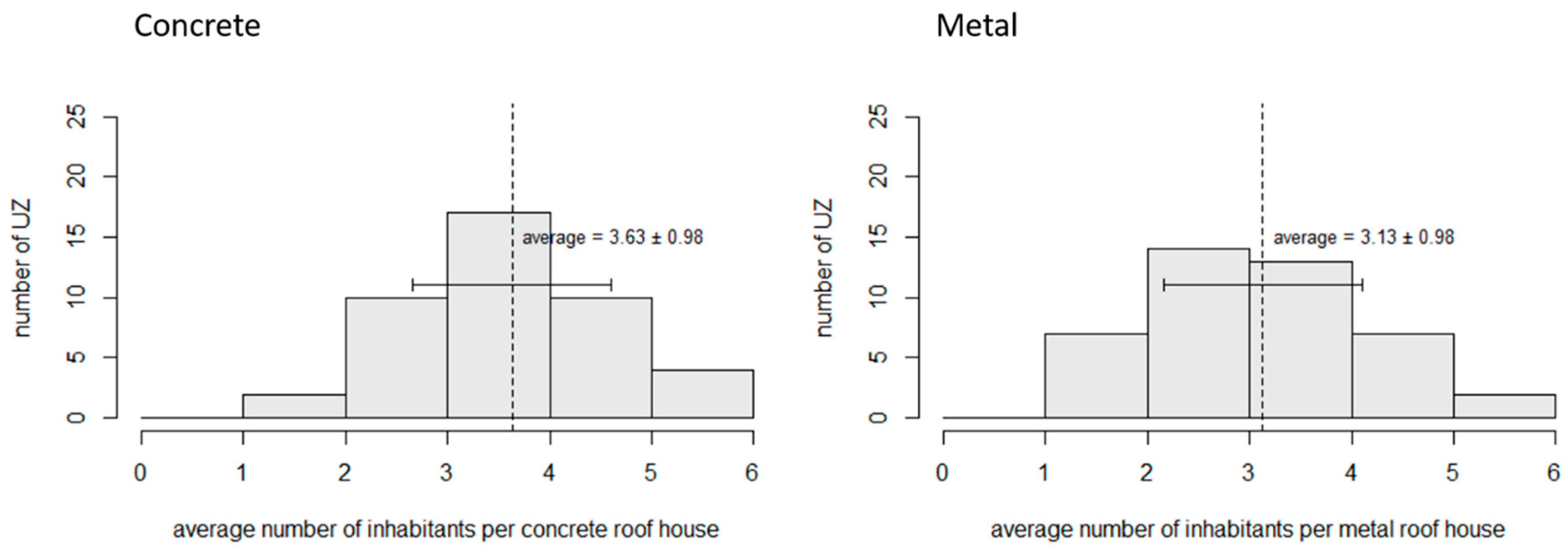
Making a distinction between buildings with different roof types, we found out that, based on our fieldwork, on average 3.63 ± 0.98 people resided in buildings with CON roofs (Figure 5), 3.01 ± 1.11 people resided in buildings with NMET roofs, and 3.23 ± 1.21 people in buildings with OMET roofs. Welch’s t-test was performed to test for significant differences in the average number of residents, in buildings of different types. No significant difference could be found between the average number of residents in NMET and OMET houses (p-value > 0.05). This is the reason why the population estimations for NMET and OMET were merged into one new category, namely metal sheet roofs (MET). The average number of residents in these type of houses is 3.13 ± 0.98 (Figure 5). A significant difference was observed between the number of residents in metal sheet roof houses and in houses with concrete roofs (p-value ≤ 0.05).
So, on average more residents are found in buildings with a concrete roof than in buildings with a metal roof. According to the census of 2003, household size increased with an increase of employed people (see also Section 2.1.1). If one assumes that employed people can more easily afford the construction of a house with a concrete roof, this may explain why overall concrete houses had a higher number of residents. Based on our fieldwork, we also analyzed if household size might be influenced by features of the built-up area, such as size, building density, accessibility, shortest distance of a house to other houses in the neighborhood, which could be easily defined from the remote sensing data for each visited UZ. We concluded that the number of residents per building was not significantly influenced by any of these spatial variables, but solely by the type of building, as characterized by its roof type.
3.2. Building and Roof Type Mapping
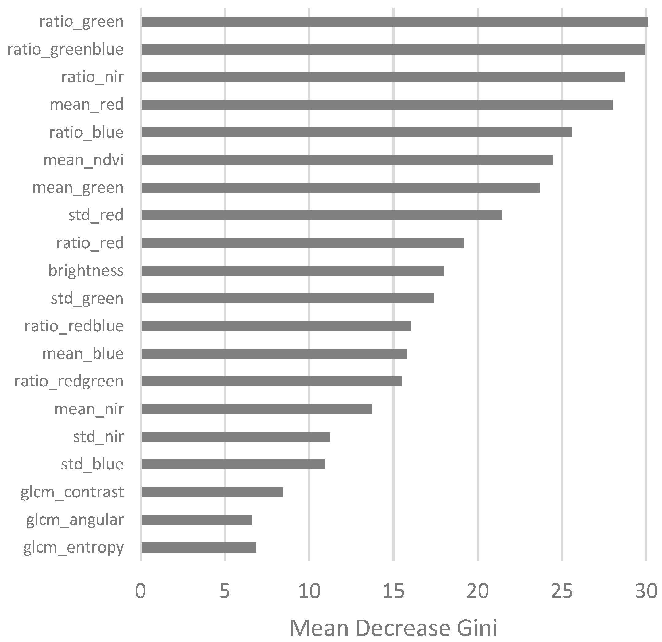
Over 55,000 buildings were manually digitized as point locations, through visual interpretation of the Pléiades images. By overlaying these point locations with the object-based land cover classification, a land cover class label was assigned to each building. As can be seen in Figure 6, the Mean Decrease Gini, which indicates the importance of each variable in the random forest classification process; shows that the most important variables contributing to the separation of the six land-cover classes in this study are spectral variables, such as the ratio green, NIR and blue, the ratio green/blue, and the mean red. Textural variables (standard deviation of spectral bands, metrics derived from the GLCM) proved to have less importance in the classification process than spectral variables. It should be noted though, that the order of importance of the variables might be different when using other segmentation parameters [40], and is also dependent on application context (study area, sensor data used).
Based on a random sample of image segments, including a building point location, the accuracy of roof type extraction was assessed. Table 2 shows the error matrix, comparing the roof type for each building defined in the validation set, against the land cover label assigned by the classifier. The validation indicated an overall classification accuracy of 75%. As can be noticed, the producer’s accuracies for the three roof types range from 0.80 for concrete roofs (CON), to 0.64 for old metal roofs (OMET), and 0.72 for new metal roofs (NMET). Buildings with OMET and NMET roofs were frequently assigned to CON by the classifier. The opposite occurred less frequently. This implied that the number of buildings with metal roofs was likely to be underestimated by the classifier. In some cases, building segments were assigned by the classifier to the non-building classes: vegetation, bare soil, or asphalt (VEG, BSO, ASP). This may have been due to (1) errors in the delineation of the image segments, leading to the presence of building, as well as non-building, land cover within the same segment; (2) some degree of spectral confusion between roof types and other land cover classes. Applying the misclassification correction procedure explained in Section 2.5, the majority of the buildings in the study area had a concrete roof (45%), followed by buildings with new metal sheet roofs (41%). A minority of the buildings had an old metal sheet roof (14%).
Based on our mapping results, the proportion of concrete roof houses seemed to have doubled since the 2003 census observations, going from 22% (2003 census) to 45% (2013 classification results). This increase is also confirmed by the field survey data of 2016. One explanation for this sudden increase were the lahar events that followed two mildly explosive eruptions at Karthala in 2005, remobilizing the ash deposits emplaced around the summit area and making them more accessible for exploitation, thus decreasing the price of the raw material and facilitating the construction of concrete houses [48]. Another explanation is that concrete houses were increasingly preferred by the local population. Use of concrete is more sustainable compared to the use of metal sheets, which get rusty by the years. Concrete houses also offer more protection against heat during the day and are considered a symbol of achievement in the Comorian society.
3.3. Population Estimation
The population estimation model proposed in this study was first applied to the 42 visited UZ, to enable validation using the leave-one-out method. For each UZ, the number of buildings of each type obtained by combining the building layer (Figure 7b) with the results of object-based classification (Figure 7c,d), was first corrected by applying the inverse calibration approach, before being multiplied with the average number of residents per building type, calculated as the mean of the average household sizes observed in the other 41 UZ (Equation (2); Figure 7e). In addition to this population estimate, for each UZ a measure of the uncertainty involved in the assessment was calculated, applying (Equation (3); Figure 7f). Estimated population was then compared with the population observed in the field in 2016 (Equations (4) and (5)).
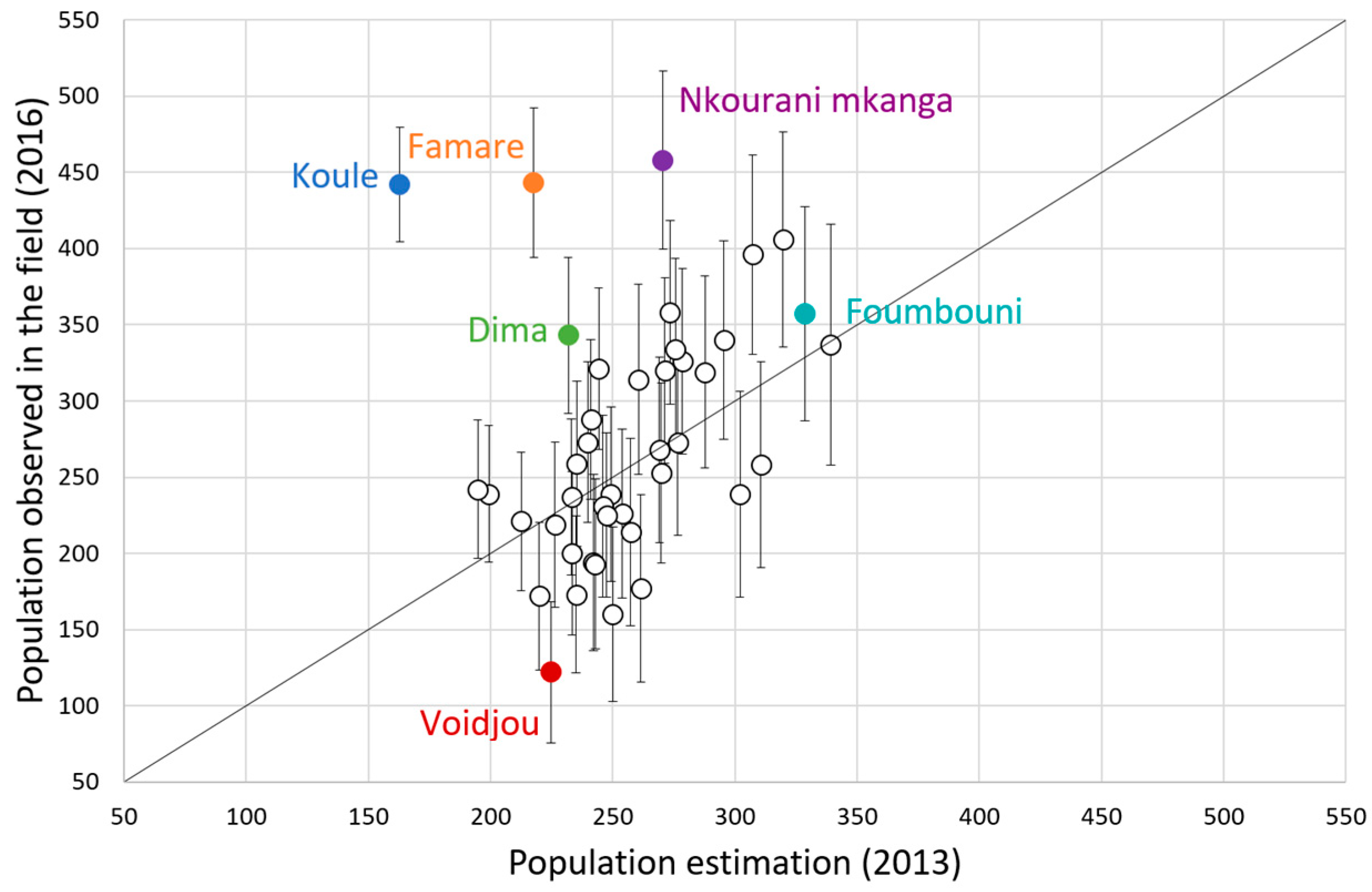
Taking model uncertainty into account, for most UZ, the reference population falls within one standard deviation of the estimated population value (Figure 8). For some UZ (e.g., Koule, Famare, Dima, Nkourani mkanga), an underestimation of observed population numbers was obtained. This type of error may be partly attributed to the development of new houses, which were not present during the acquisition of the remotely sensed imagery in 2013, as well as to the absence of houses in the building layer that were located under trees and were not visible in the remotely sensed images. The overestimation of the population for Voidjou (Figure 8), can be explained by the specificity of the neighborhood. This UZ hosts a large portion of immigrants, with household characteristics strongly deviating from the general trend on the island (only 1.91 people reside in buildings with CON roofs and 1.81 people in MET roofs).
Calculation of the proportional prediction errors showed a negligible model bias (es = −0.03) and a magnitude of the error ABS(es) = 0.17. The distributional dispersion of the bias and the magnitude of the error, indicated by the interquartile range, were 0.32 and 0.17, respectively. This indicated that there was quite some uncertainty involved in the population estimation process.
3.4. Model Extrapolation and Comparison with Census Prediction
The model calibrated on the 42 visited UZ was applied to the entire area covered by the Pléiades images (Figure 4). After extracting, for each UZ, the number of houses and defining their type through object-based classification, the inverse calibration approach discussed in Section 2.5, was applied for dealing with misclassification bias in roof type discrimination. The method corrects for the confusion that exists between the CON and MET classes and allows assigning a roof type (CON or MET) to buildings that have been wrongly assigned to a non-building classes (VEG, BSO and ASP). The number of buildings allocated to a new class through the calibration procedure varies between UZ, and is shown for the capital Moroni and its surroundings in Figure 9a. Figure 9b shows the population estimation results, for the UZ of the capital Moroni, and their corresponding standard deviation (Figure 9c). As expected, the standard deviation of the population estimate was low for areas with lower population numbers and higher for densely populated areas.
Aggregating the population estimates for the UZ to the village level for the entire study area, and comparing them with the 2013 population estimates from the 2003 census, which were based on a hypothetical growth rate [37], shows a good linear fit (Figure 10); yet estimated population numbers were systematically lower than the ones predicted by the 2003 census. Not including the capital Moroni, which has a much higher population compared to the other villages, an R2 value of 0.88 was obtained, which implied that a large part of the variation in the 2013 census predictions is explained by the proposed model. The difference between our results and those predicted by the census, are most likely due to uncertainties about the expected growth rate used by the National Census Direction.
4. Discussion
The modelling approach proposed in this paper combined high resolution image interpretation with targeted fieldwork to assess population at neighborhood level, for regions for which no population data are available (Figure 7e and Figure 9b). The model proposed assumed that the average number of residents per building type was relatively stable. To deal with the observed variation in average number of residents per building between different UZ, population estimates for each UZ were accompanied by a measure of uncertainty. If the variation in the number of residents per building type among different UZ is higher, the uncertainty of the population estimate at UZ level will increase. The uncertainty of the population estimation at UZ level will also increase with the number of residents per UZ.
Comparison of estimated population, for the 42 visited UZ with population numbers observed in the field (Figure 8), shows some systematic over- and underestimations of population, which can be related to limitations in the approach proposed. Some of these limitations had to do with remote sensing image interpretation. Even though high spatial resolution imagery was used in this study for identifying building structures, visual interpretation was to some extent error-prone. First of all, new houses developed in the period between image acquisition and field work could not be identified from the Pléiades imagery (e.g., Famare, Dima, Nkourani mkanga, Foumbouni; Figure 11). Moreover, houses partly or fully covered by trees could not always be identified in the imagery (e.g., Koule; Figure 11). As such, underestimation of the actual number of population was likely in some UZ (Figure 8). Foumbouni household characteristics strongly deviated from the general trend on the island, which explained why, despite a clear underestimation of the number of houses, no underestimation of the population was obtained for this outlier, (Figure 8) (on average, CON houses in the Foumbouni UZ host 2.87 people and MET houses 2.12 people).
Errors in roof type classification also affected the results obtained with our model. To limit the impact of these errors on population predictions, an inverse calibration procedure was applied to correct building counts obtained for different roof types, using information obtained from the classification’s error matrix. This approach is commonly used to correct estimates of the total area of different cover types in land cover maps, obtained through image interpretation [44,45,46]. Using this method, the relative fraction of buildings with concrete and metal roofs within the study area, which based on the original image interpretation was 45.6% for CON and 49.4% for MET (5% of the buildings were wrongly assigned to classes that do not belong to roof type classes), changed to 45% and 55%, respectively. It should be kept in mind though, that the error matrix only provides a global estimate of spectral confusion among land cover classes, which may not necessarily be representative of the classification errors occurring within one particular UZ. As such, the correction method cannot avoid that some local bias in the estimated number of buildings of different type may occur.
Another issue affecting the results was that when identifying buildings from the remotely sensed imagery, it was mostly not possible to obtain information on the function of the building or on its current use (e.g., vacant versus non-vacant buildings). This is why, when calculating the average number of residents per building through fieldwork, all buildings were taken in account, irrespective of their use. While this approach ensures that the population estimation implicitly accounts for the fact that a certain amount of building space in each UZ is not used for residential purposes, it is likely to lead to overestimation of the population in UZs where the share of non-residential use or vacant buildings is high, and vice versa. The proposed measure of uncertainty incorporates this effect.
While in our study not much variation in building height was observed, including height of buildings in the modelling might further improve the model performance, especially in regions where clear differences in building height are present. The increasing availability of high resolution remotely sensed data, including for data poor regions, holds great potential for further refining population estimation approaches relying on combining remote sensing with field work, as proposed in this study.
Considering that the average number of residents for concrete and metal roof buildings proved to be significantly different (p-value ≤ 0.05), we decided to incorporate housing type in our population estimation model. The question remains though if distinguishing between different roof types improves the predictive accuracy of the modelling. This will obviously depend on the degree to which the average number of residents in both types of buildings differs, yet it will also depend on differences in the share of both types of buildings at the level of each UZ, as well as on uncertainties involved in the modelling, including uncertainty caused by difficulties in roof type discrimination (see above). A slight improvement was observed in the population estimation per UZ, when integrating roof type discrimination in the model (es = −0.03 and ABS(es) = 0.17), compared to a simplified model not distinguishing different building types (es = −0.04 and ABS(es) = 0.15). This slight difference in model performance may have been largely attributed to the relatively small difference in average number of residents for concrete and metal roof buildings, compared to the variance of both distributions. Whilst a significant difference was observed, the p-value was only slightly below 0.05 (p-valuecon-met = 0.02). Although in this case study incorporating roof type in the population estimation model did not substantially improve prediction accuracy, compared to a model not distinguishing between different type of buildings; the modelling framework proposed will be useful in regions where differences in average number of residents for different types of houses are more substantial, and where the number of buildings of different types strongly differs between different urban zones.
5. Conclusions
Organizing a census is not an easy task and requires a high investment in resources, especially for developing countries which have more urgent priorities. This explains partially, why in many places in the world detailed population counts are not available on a ten-yearly basis. In this study, we explored the potential of high spatial resolution remotely sensed imagery, in combination with dedicated fieldwork, as a fast and less costly alternative for providing timely information on population numbers and population distribution. A population estimation model was defined, associating the number of houses of different types found within each neighborhood, obtained through remote sensing, with the average number of residents per building type, obtained through fieldwork.
As a first step in the approach, buildings were manually identified from high spatial resolution Pléiades imagery. An object-based classification approach was used to automatically detect the roof type of each building from the image data. To correct for bias in the count of buildings with different roof types, due to spectral confusion between different materials, an inverse calibration procedure was applied. Population estimation at the level of pre-defined urban zones was accomplished by combining corrected building counts, obtained through remote sensing, with estimates of the average number of residents per building type, collected in the field for a sample of urban zones. For each urban zone, an indication of the uncertainty of the estimate was provided, considering the observed variability in average household size per urban zone. Validation of the model at the neighborhood level, revealed low model bias and a relative error at the urban zone level of 17%. Comparison with a model not distinguishing between different types of buildings, showed that in the present case study, the added value of including building type in the modelling seems to be limited. This could be explained by the difference in the average number of residents per building type being relatively small in the study area, and by the fact that the number of buildings of different types did not show a strong variation between different urban zones. In these circumstances the advantages of discriminating between different building types do not weigh up against the additional uncertainty introduced into the modelling. The modelling framework proposed, may prove useful though in regions with more outspoken differences in the average number of residents, for different type of houses, and with stronger contrasts in urban morphology. While in this case study locations of individual dwellings where manually pin-pointed on the high-resolution imagery, cost and time required for data collection might be substantially reduced in areas where a building data layer would already be available. With the increasing availability of volunteered geographic information, it would be interesting to test the method proposed in combination with these new data sources.
Author Contributions
Conceptualization, S.M. and F.C.; Data curation, S.M.; Formal analysis, S.M. and F.C.; Funding acquisition, S.M.; Investigation, S.M. and F.C.; Methodology, S.M. and F.C.; Project administration, S.M.; Resources, S.M., H.S. and F.C.; Software, S.M.; Supervision, S.M., M.K. and F.C.; Validation, S.M., M.K., H.S. and F.C.; Visualization, S.M.; Writing—original draft, S.M.; Writing—review & editing, S.M., M.K., H.S. and F.C.
Funding
This research received no external funding.
Acknowledgments
We are extremely grateful to the “Centre National de Documentation et de Recherche Scientifique”, for its technical support during the three missions done on Ngazidja Island. Many thanks to Shafik Bafakih for his assistance, and for sharing his expertise during these missions. The authors also would like to thank Marc Van Molle and the “Fonds Wetenschappelijk Onderzoek”, for their financial support. We want to thank Astrium Services for allowing us to use the Pléiades imageries acquired of the island, thanks to a license for technical evaluation purposes. Thank you to COOPI and Z_GIS, for providing us with the high spatial resolution Digital Elevation Model of the southern part of Ngazidja Island. Thank you to all Comorian institutions for sharing information with us making this research possible, and to the Comorian students (Raissa Binti, Daroueche Ali Hila, Hamada Soilihi, Gomes Mohamed, Ahamada Moinahalima, Fahmiya Ismael, Hidaya Mansouri, Sefoudine Soilihi, Andhumou Mze, Nayel Somadou, Wardou Iboursi, Abdjad Youssouf, Mouzda Issa) for their help with data collection. Thank you to my colleagues Frederik Priem, Kasper Cockx, Inge Meyskens, and Sam Poppe, for helping me with the digitizing work. Special thanks to Sam Poppe, for sharing with me his stories and expertise about Ngazidja Island, and for reviewing this paper.
Conflicts of Interest
The authors declare no conflict of interest.
References
- Chen, K.; McAneney, J.; Blong, R.; Leigh, R.; Hunter, L.; Magill, C. Defining area at risk and its effect in catastrophe loss estimation: A dasymetric mapping approach. Appl. Geogr. 2004, 24, 97–117. [Google Scholar] [CrossRef]
- Kayembe wa Kayembe, M.; Ngoy Ndombe, A.; Makanzu Imwangana, F.; Mpinda, M.; Misilu Mia Nsokimieno, E.; Wolff, E. Contribution of Remote Sensing in the Estimation of the Populations Living in Areas with Risk of Gully Erosion in Kinshasa (D. R. Congo). Case of Selembao Township. Am. J. Geosci. 2016, 6, 71–79. [Google Scholar] [CrossRef]
- Tomás, L.; Fonseca, L.; Almeida, C.; Leonardi, F.; Pereira, M. Urban population estimation based on residential buildings volume using IKONOS-2 images and lidar data. Int. J. Remote Sens. 2016, 37, 1–28. [Google Scholar] [CrossRef]
- Dong, P.; Ramesh, S.; Nepali, A. Evaluation of small-area population estimation using LiDAR, Landsat TM and parcel data. Int. J. Remote Sens. 2010, 31, 5571–5586. [Google Scholar] [CrossRef]
- United Nations. Principles and Recommendations for Population and Housing Censuses; United Nations Publication: New York, NY, USA, 2015; Volume 67, ISBN 978-92-1-161597-5. [Google Scholar]
- Statistics Netherlands. Dutch Census 2011: Analysis and Methodology; Statistics Netherlands: The Hague, The Netherlands, 2014; ISBN 9789035719484.
- Deng, C.; Wu, C.; Wang, L. Improving the housing-unit method for small-area population estimation using remote-sensing and GIS information. Int. J. Remote Sens. 2010, 31, 5673–5688. [Google Scholar] [CrossRef]
- Joseph, M.; Wang, L.; Wang, F. Using Landsat imagery and census data for urban population density modeling in Port-au-Prince, Haiti. GISci. Remote Sens. 2012, 49, 228–250. [Google Scholar] [CrossRef]
- Li, G.; Weng, Q. Using Landsat ETM+ imagery to measure population density in Indianapolis, Indiana, USA. Photogramm. Eng. Remote Sens. 2005, 71, 947–958. [Google Scholar] [CrossRef]
- Lo, C.P. Zone-Based Estimation of Population and Housing Units from Satellite-Generated Land Use/Land Cover Maps; Victor, M., Ed.; Taylor and Francis: London, UK; New York, NY, USA, 2003; ISBN 0415260450. [Google Scholar]
- Lo, C.P.; Chan, H.F. Rural population estimation from aerial photographs. Photogramm. Eng. Remote Sens. 1980, 46, 337–345. [Google Scholar]
- Lu, D.; Weng, Q.; Li, G. Residential population estimation using a remote sensing derived impervious surface approach. Int. J. Remote Sens. 2006, 27, 3553–3570. [Google Scholar] [CrossRef]
- Weber, E.M.; Seaman, V.Y.; Stewart, R.N.; Bird, T.J.; Tatem, A.J.; McKee, J.J.; Bhaduri, B.L.; Moehl, J.J.; Reith, A.E. Census-independent population mapping in northern Nigeria. Remote Sens. Environ. 2018, 204, 786–798. [Google Scholar] [CrossRef] [PubMed]
- Wu, S.; Qiu, X.; Wang, L. Population estimation methods in GIS and remote sensing: A review. GISci. Remote Sens. 2005, 42, 58–74. [Google Scholar] [CrossRef]
- Yagoub, M.M. Application of remote sensing and Geographic Information Systems (GIS) to population studies in the gulf: A case of Al Ain city (UAE). J. Indian Soc. Remote Sens. 2006, 34, 7–21. [Google Scholar] [CrossRef]
- Zhu, H.; Li, Y.; Liu, Z.; Fu, B. Estimating the population distribution in a county area in China based on impervious surfaces. Photogramm. Eng. Remote Sens. 2015, 81, 155–163. [Google Scholar] [CrossRef]
- Mahabir, R.; Croitoru, A.; Crooks, A.; Agouris, P.; Stefanidis, A. A Critical Review of High and Very High-Resolution Remote Sensing Approaches for Detecting and Mapping Slums: Trends, Challenges and Emerging Opportunities. Urban Sci. 2018, 2, 8. [Google Scholar] [CrossRef]
- Kuffer, M.; Pfeffer, K.; Sliuzas, R. Slums from Space—15 Years of Slum Mapping Using Remote Sensing. Remote Sens. 2016, 8, 455. [Google Scholar] [CrossRef]
- Yu, S.; Zhang, Z.; Liu, F. Monitoring population evolution in China using time-series DMSP/OLS nightlight imagery. Remote Sens. 2018, 10, 194. [Google Scholar] [CrossRef]
- Jaiswal, R.K.; Arunachalam, A.; Diwakar, P.G. Potential of High Resolution Satellite Data for Human Population Estimation. Asian J. Geoinf. 2015, 15, 1–8. [Google Scholar]
- Ayila, A.E.; Paul Babatunde, B.; Yohanna, J.P. Population estimation and census track demarcation in Hwolshe, Plateau State, Nigeria: A geospatial approach. Remote Sens. Appl. Soc. Environ. 2018, 10, 183–189. [Google Scholar] [CrossRef]
- Briggs, D.J.; Gulliver, J.; Fecht, D.; Vienneau, D.M. Dasymetric modelling of small-area population distribution using land cover and light emissions data. Remote Sens. Environ. 2007, 108, 451–466. [Google Scholar] [CrossRef]
- Tan, M.; Li, X.; Li, S.; Xin, L.; Wang, X.; Li, Q.; Li, W.; Li, Y.; Xiang, W. Modeling population density based on nighttime light images and land use data in China. Appl. Geogr. 2018, 90, 239–247. [Google Scholar] [CrossRef]
- Liu, X.; Clarke, K.; Herold, M. Population density and image texture: A comparison study. Photogramm. Eng. Remote Sens. 2006, 72, 187–196. [Google Scholar] [CrossRef]
- Hillson, R.; Alejandre, J.D.; Jacobsen, K.H.; Ansumana, R.; Bockarie, A.S.; Bangura, U.; Lamin, J.M.; Malanoski, A.P.; Stenger, D.A. Methods for Determining the Uncertainty of Population Estimates Derived from Satellite Imagery and Limited Survey Data: A Case Study of Bo City, Sierra Leone. PLoS ONE 2014, 9, e112241. [Google Scholar] [CrossRef] [PubMed]
- Veljanovski, T.; Urša, K.; Pehani, P.; Oštir, K.; Kovačič, P. Object-Based Image Analysis of VHR Satellite Imagery for Population Estimation in Informal Settlement Kibera-Nairobi, Kenya. Intech Open 2018, 2, 64. [Google Scholar] [CrossRef]
- Checchi, F.; Stewart, B.T.; Palmer, J.J.; Grundy, C. Validity and feasibility of a satellite imagery-based method for rapid estimation of displaced populations. Int. J. Health Geogr. 2013, 12, 4. [Google Scholar] [CrossRef] [PubMed] [Green Version]
- Pesaresi, M.; Kemper, T.; Gueguen, L.; Soille, P. Automatic information retrieval from meter and sub-meter resolution satellite image data in support to crisis management. IEEE Geosci. Remote Sens. Symp. 2010, 25, 1792–1795. [Google Scholar] [CrossRef]
- Li, X.; Shao, G. Object-based land-cover mapping with high resolution aerial photography at a county scale in midwestern USA. Remote Sens. 2014, 6, 11372–11390. [Google Scholar] [CrossRef]
- Myint, S.W.; Gober, P.; Brazel, A.; Grossman-Clarke, S.; Weng, Q. Per-pixel vs. object-based classification of urban land cover extraction using high spatial resolution imagery. Remote Sens. Environ. 2011, 115, 1145–1161. [Google Scholar] [CrossRef]
- Füreder, P.; Hölbling, D.; Tiede, D.; Zeil, P.; Lang, S. Monitoring refugee camp evolution and population dynamics in Dagahaley, Kenya, based on VHR satellite data. In Proceedings of the 9th Internation Conference African Association Remote Sensing Environment, El Jadida, Morocco, 29 October–2 November 2012. [Google Scholar]
- Li, J.; Li, Y.; Chapman, M.A.; Rüther, H. Small Format Digital Imaging for Informal Settlement Mapping. Photogramm. Eng. Remote Sens. 2005, 71, 435–442. [Google Scholar] [CrossRef]
- Tiede, D.; Lang, S.; Hölbling, D.; Füreder, P. Transferability of obia rulesets for idp camp analysis in darfur. Geobia 2010, 2006. [Google Scholar]
- Mitchell, S.; Andersson, N.; Ansari, N.M.; Omer, K.; Soberanis, J.L.; Cockcroft, A. Equity and vaccine uptake: A cross-sectional study of measles vaccination in Lasbela District, Pakistan. BMC Int. Health Hum. Rights 2009, 9 (Suppl. 1), S7. [Google Scholar] [CrossRef]
- Adah, M.I.; Taiwo, A.T. Multidimensional Poverty in Rural Kogi State, Nigeria: A Subjective Wellbeing (SWB) Approach. Science 2017, 5, 13–19. [Google Scholar]
- The Housing Development Agency. Working for Integration—Annual Report 2012–2013; The Housing Development Agency: Limpopo, South Africa, 2017. [Google Scholar]
- DGSP; ICF. Enquête Démographique et de Santé et à Indicateurs Multiple aux Comores 2012; DGSP: Moroni, Comoros, 2014. [Google Scholar]
- Commissariat Général au Plan. Analyse des Données du Recensement Général de la Population et de L’habitat 2003: Ménages et Habitations; Commissariat Général au Plan: Moroni, Comoros, 2007. [Google Scholar]
- Trimble eCognition. Developer 9.0 Reference Book; Trimble eCognition: Munich, Germany, 2014; pp. 1–266. [Google Scholar]
- Salas, E.; Boykin, K.; Valdez, R. Multispectral and Texture Feature Application in Image-Object Analysis of Summer Vegetation in Eastern Tajikistan Pamirs. Remote Sens. 2016, 8, 78. [Google Scholar] [CrossRef]
- Frohn, R.C.; Autrey, B.C.; Lane, C.R.; Reif, M. Segmentation and object-oriented classification of wetlands in a karst Florida landscape using multi-season Landsat-7 ETM+ imagery. Int. J. Remote Sens. 2011, 32, 1471–1489. [Google Scholar] [CrossRef]
- De Roeck, T.; Van de Voorde, T.; Canters, F. Full hierarchic versus non-hierarchic classification approaches for mapping sealed surfaces at the rural-urban fringe using high-resolution satellite data. Sensors 2009, 9, 22–45. [Google Scholar] [CrossRef] [PubMed]
- Witharana, C.; Civco, D.L.; Meyer, T.H. Evaluation of data fusion and image segmentation in earth observation based rapid mapping workflows. ISPRS J. Photogramm. Remote Sens. 2014, 87, 1–18. [Google Scholar] [CrossRef]
- Czaplewski, R.L.; Catts, G.P. Calibration of remotely sensed proportion or area estimates for misclassification error. Remote Sens. Environ. 1992, 39, 29–43. [Google Scholar] [CrossRef]
- Walsh, T.A.; Burk, T.E. Calibration of satellite classifications of land area. Remote Sens. Environ. 1993, 46, 281–290. [Google Scholar] [CrossRef]
- Canters, F. Evaluating the uncertainty of area estimates derived from fuzzy land-cover classification. Photogramm. Eng. Remote Sens. 1997, 63, 403–414. [Google Scholar]
- Cockx, K.; Canters, F. Incorporating spatial non-stationarity to improve dasymetric mapping of population. Appl. Geogr. 2015, 63, 220–230. [Google Scholar] [CrossRef]
- Morin, J. Gestion Institutionnelle et Réponses des Populations Face Aux Crises Volcaniques: Études de Cas à La Réunion et en Grande Comore; Université de la Réunion: La Réunion, France, 2012. [Google Scholar]
Figure 1.
Population repartition on Ngazidja Island (Indian Ocean) at the level of individual villages, based on the last census realized in 2003.
Figure 1.
Population repartition on Ngazidja Island (Indian Ocean) at the level of individual villages, based on the last census realized in 2003.
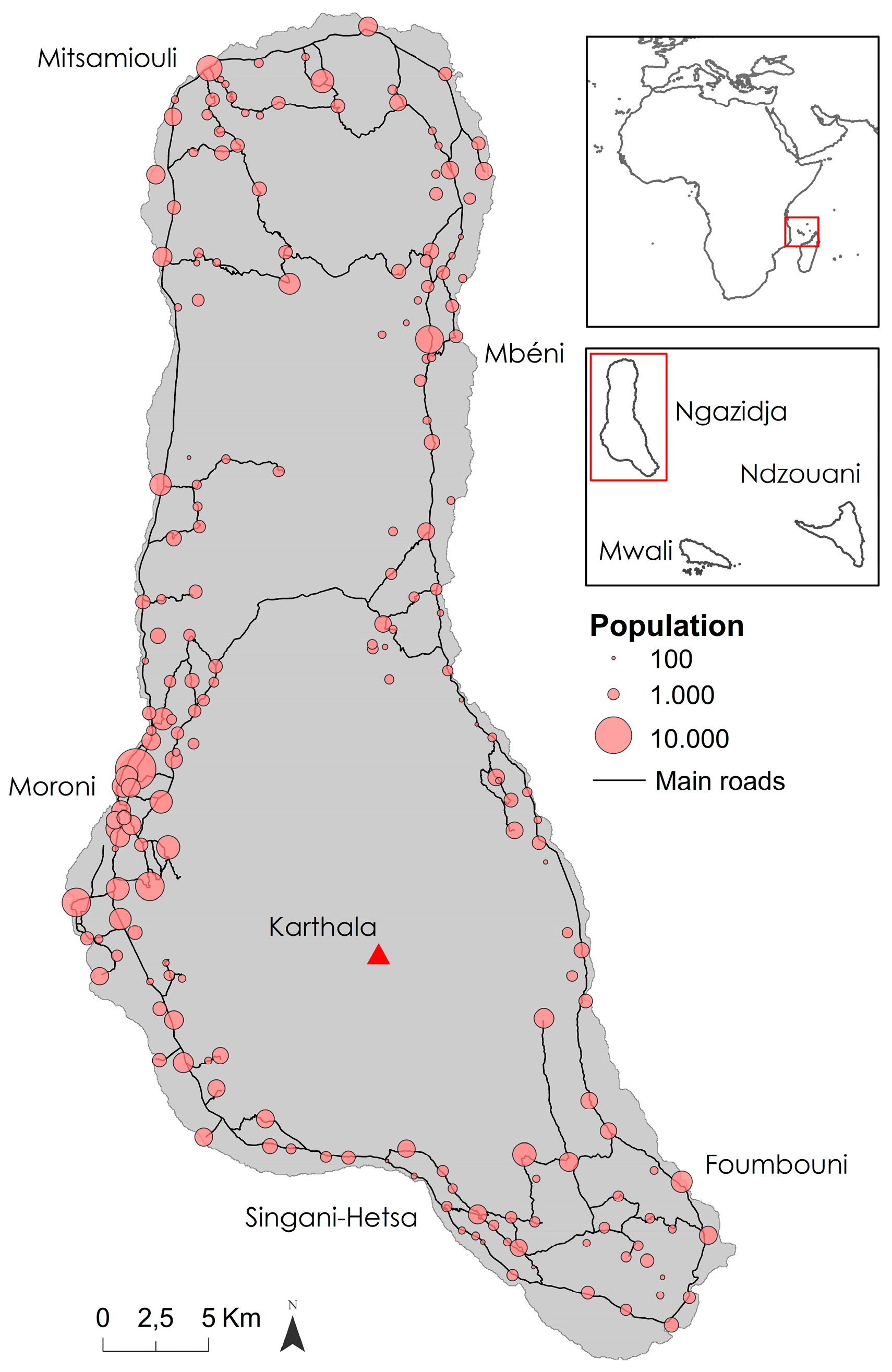
Figure 2.
Different types of dwellings present on Ngazidja Island. The dwellings differ through the building material used: (a) plant material house, (b) new metal sheet house, (c) old metal sheet house, and (d) concrete house.
Figure 2.
Different types of dwellings present on Ngazidja Island. The dwellings differ through the building material used: (a) plant material house, (b) new metal sheet house, (c) old metal sheet house, and (d) concrete house.

Figure 3.
“Urban Zones” (UZ) are built-up areas delineated by the road network, which are representative of neighborhoods. To collect information about the number of residents and type of dwelling they are living in, large urban areas dense and less dense UZ have been visited (shown in red). Through the methodology, population in all (grey bounded) UZ will be estimated. Example of the UZ delineated in Vouvouni, in the Bambao district.
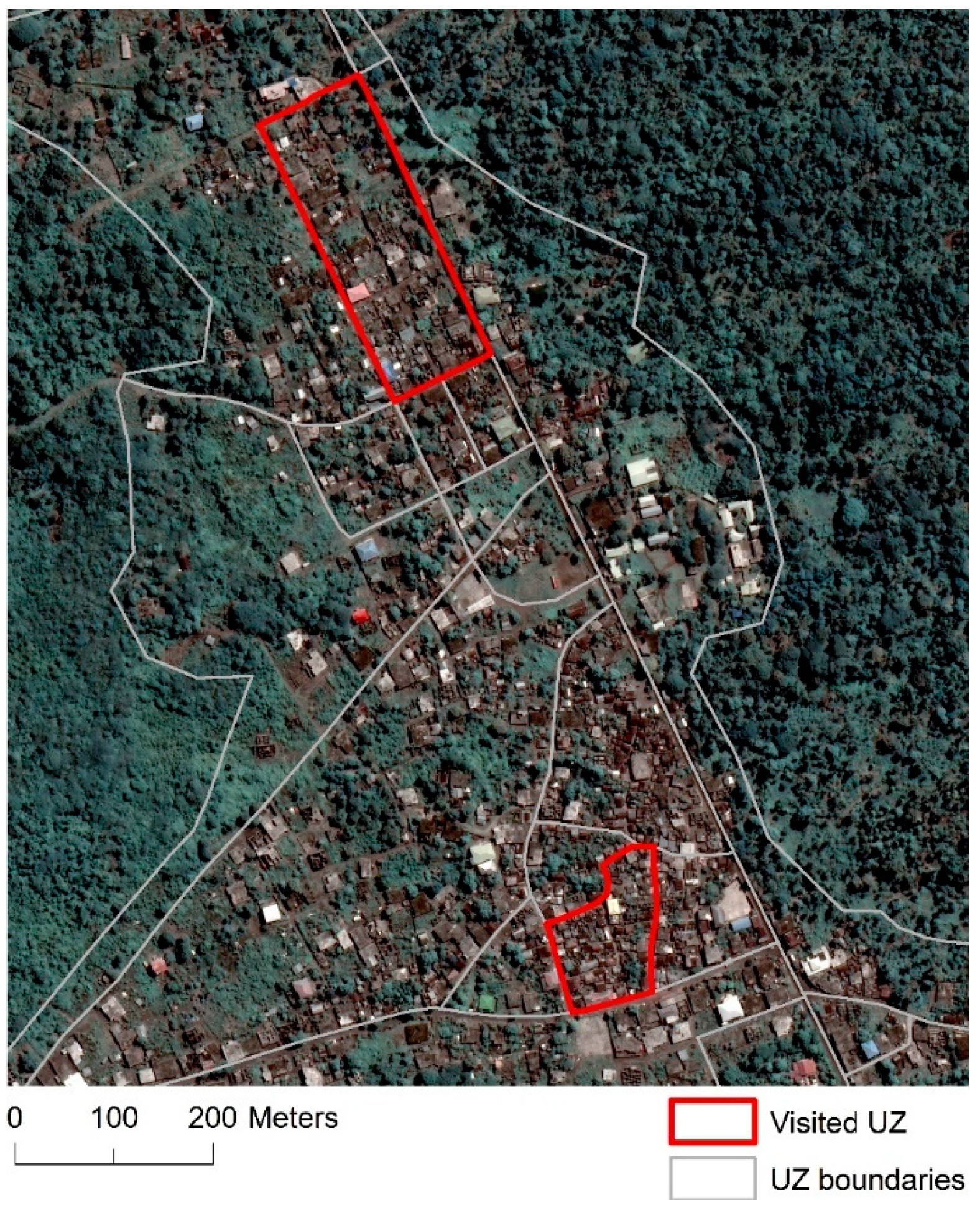
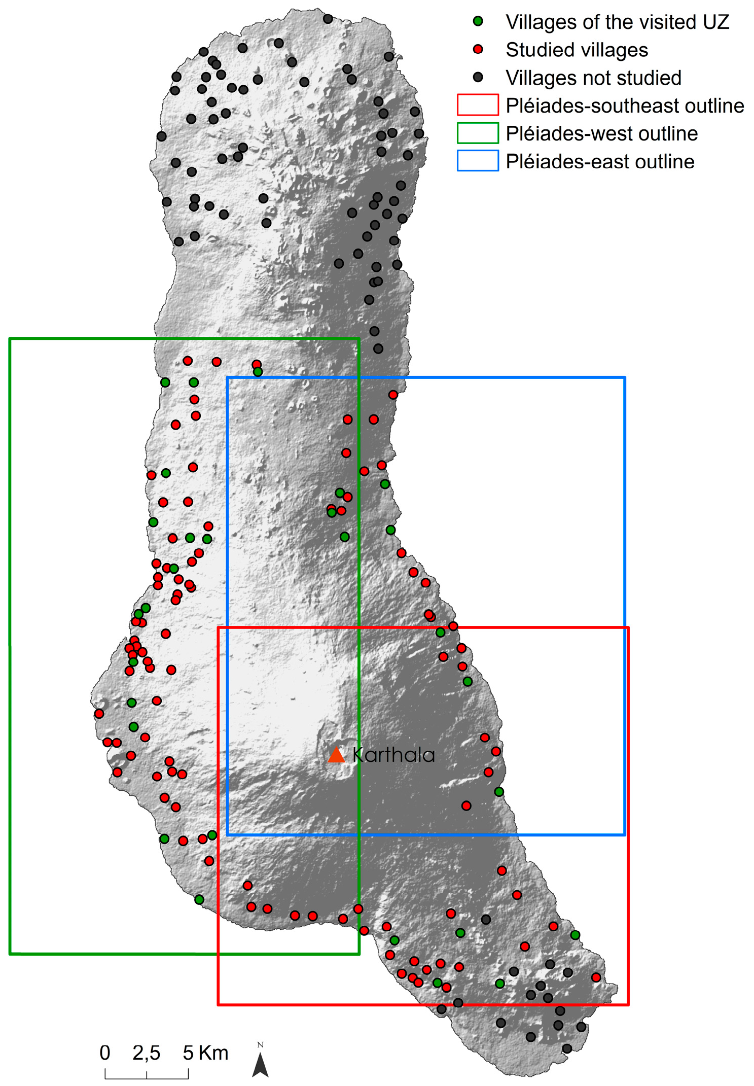
Figure 4.
Location of the visited and studied villages. Villages not included were out of the limits of the Pléiades images used in the study, or were covered by clouds, or in their shadow at the moment of image acquisition.
Figure 4.
Location of the visited and studied villages. Villages not included were out of the limits of the Pléiades images used in the study, or were covered by clouds, or in their shadow at the moment of image acquisition.

Figure 5.
Frequency distribution of the average number of inhabitants per house type. The average number of residents in buildings with concrete roofs (CON) is 3.63 ± 0.98 people, whereas 3.13 ± 0.98 people reside in buildings with metal sheet roof (MET). A significant difference in average number of inhabitants is observed between the two types of houses (p-value ≤ 0.05).

Figure 6.
Relative importance of the spectral and texture variables used in the object-based classification. The most important variables contributing to the separation of the six land-cover classes are spectral variables. Textural variables prove to have less importance in the classification process.

Figure 7.
Different steps in the estimation of the population from high resolution remotely sensed imagery. Using high-resolution 2013 Pléiades images (a), the location of buildings is defined (b). After segmentation and classification of the image (c), the roof type is automatically allocated to each building (d). Population estimation is done at a neighborhood level (e), with an assessment of uncertainty (f). Results shown are for Mitsoudje, in the Hambou district.
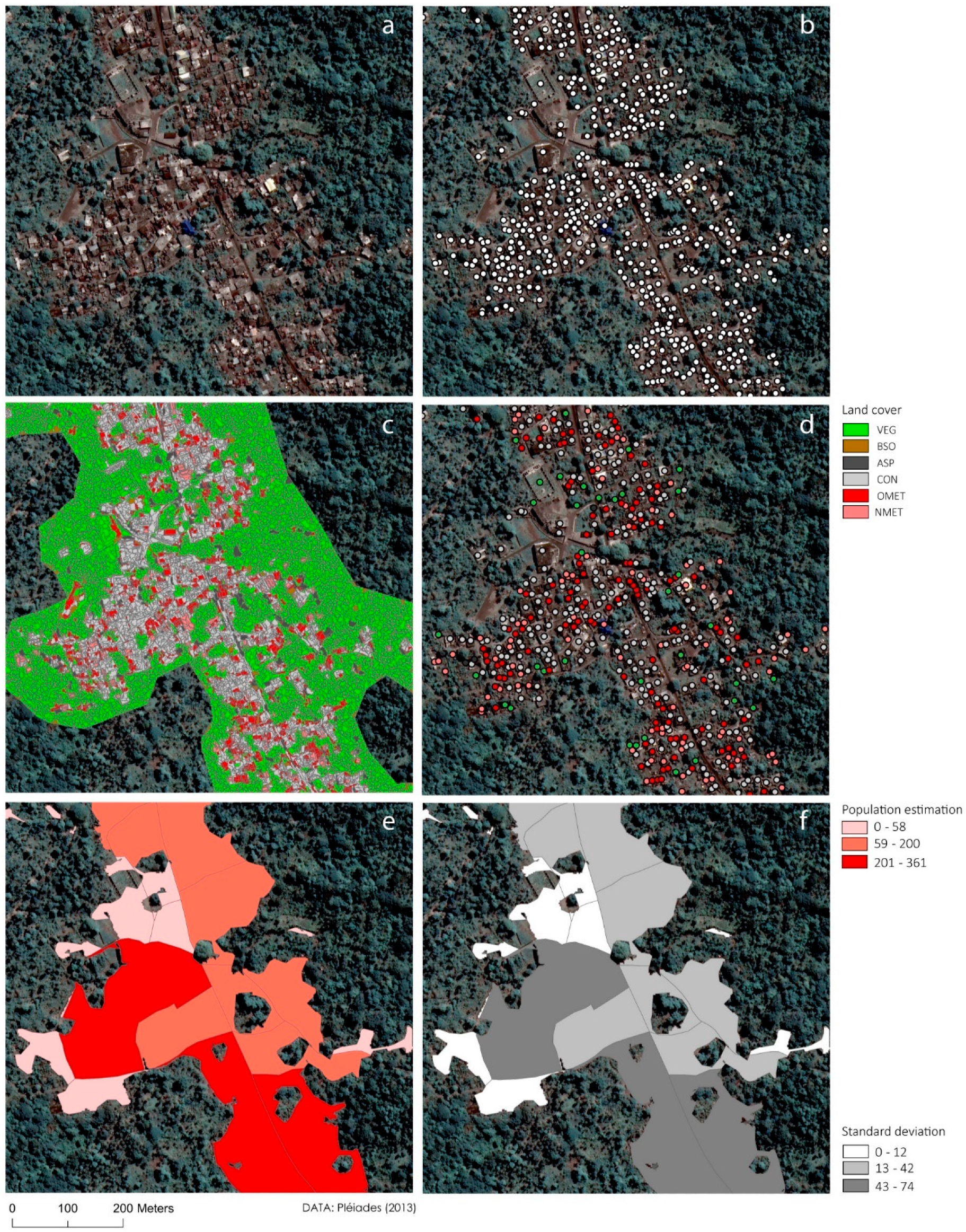
Figure 8.
Comparison of the population estimation and its standard deviation, with the population obtained by field observation for the 42 UZ visited. The solid line represents the trend 1:1 line. Population in Koule, Famare, Dima, and Nkourani mkanga is underestimated. This may be partly attributed to the development of new houses, which were not present during the acquisition of the remotely sensed imagery in 2013, and the absence of houses in the building layer that are located under trees. In Voidjou, the population is overestimated, since the UZ hosts a large portion of immigrants with household characteristics strongly deviating from the general trend on the island.

Figure 9.
(a) Number of houses that have been allocated to a new class after the inverse calibration approach to account for misclassification bias, for the UZ of Moroni. (b) Population estimates for the UZ of Moroni; (c) Standard deviation of the population estimates, for the UZ of Moroni.
Figure 9.
(a) Number of houses that have been allocated to a new class after the inverse calibration approach to account for misclassification bias, for the UZ of Moroni. (b) Population estimates for the UZ of Moroni; (c) Standard deviation of the population estimates, for the UZ of Moroni.
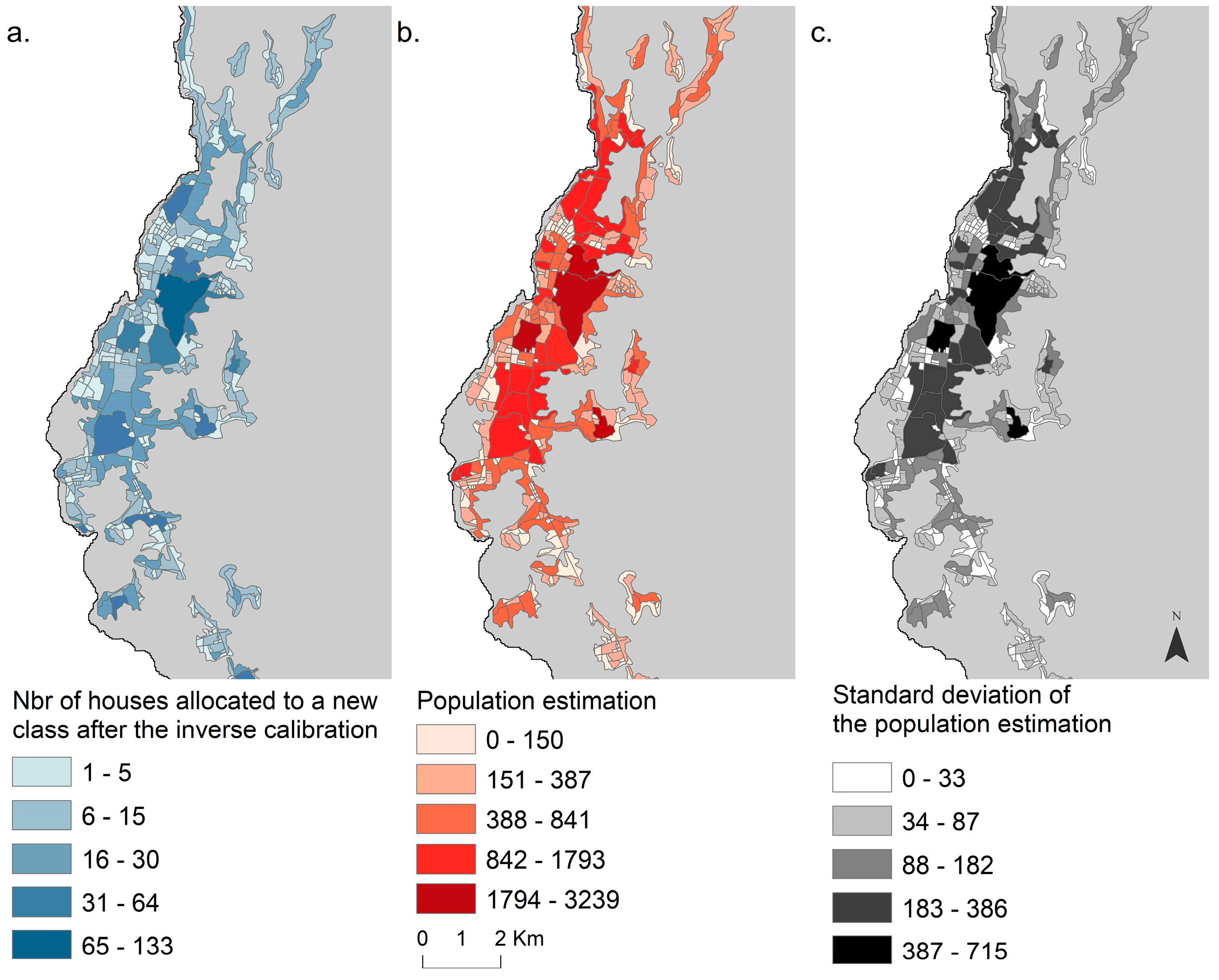
Figure 10.
Results for the model aggregated to the village level, compared with the 2013 population prediction based on the 2003 census. A good linear fit is obtained (R2 = 0.88), yet estimated population numbers are systematically lower than the ones predicted by the 2003 census. Moroni is excluded from the graph for clarity (population census prediction (2013) for Moroni = 107,912 people; population estimation prediction (2013) based on our model = 85,247 people). The solid line represents the trend 1:1 line, and the dashed line the regression line.
Figure 11.
Comparison between houses detected from remote sensing imagery and houses observed during field work. In some UZ, the number of houses detected from remote sensing images is lower than the number of houses observed in the field. The development of new houses (e.g., Famare, Dima, Nkourani mkanga, Foumbouni) or houses partly or fully covered by trees (e.g., Koule) can explain this underestimation. The solid line is the trend 1:1 line.

Table 1.
Variables used for object-based classification. Both spectral information and textural information characterizing the image objects are used in the classification.
Table 1.
Variables used for object-based classification. Both spectral information and textural information characterizing the image objects are used in the classification.
| Variables | Description | |
|---|---|---|
| Mean | blue, green, red, NIR | Mean of the values in the spectral band, calculated over all pixels within the segment |
| NDVI | Mean of (NIR-red)/(NIR + red) within the segment | |
| Ratio | blue, green, red, NIR | Ratio between the mean of the spectral band and the sum of the mean values in each band within the segment |
| green/blue, red/blue, red/green | Mean of one spectral band divided by the mean of the other band within the segment | |
| Standard deviation | blue, green, red, NIR | Standard deviation of all pixel values in the spectral band within the segment |
| Brightness | Sum of the mean values in each spectral band | |
| Grey Level Co-occurrence Matrix (GLCM) | Angular second moment | Reflects the degree of homogeneity present in the spectral band within the segment |
| contrast | Reflects the contrast present in all spectral bands within the segment | |
| entropy | Reflects the randomness in the spatial arrangement of all spectral bands values within the segment |
Table 2.
Confusion matrix of the roof type classification (defined based on 214 validation points) where VEG = vegetation, BSO = bare soil, ASP = asphalt, CON = concrete, OMET = old metal sheet, NMET = new metal sheet. The confusion observed between specific classes is further used to apply the misclassification correction procedure.
| Reference | |||||
|---|---|---|---|---|---|
| Land Cover Classes | CON | OMET | NMET | ||
| Classification | VEG | 1 | 0 | 2 | |
| BSO | 1 | 1 | 0 | ||
| ASP | 1 | 0 | 0 | ||
| CON | 76 | 5 | 23 | ||
| OMET | 7 | 14 | 2 | ||
| NMET | 9 | 2 | 70 | Overall Accuracy | |
| Producer’s Accuracy | 0.80 | 0.64 | 0.72 | 0.75 | |
© 2018 by the authors. Licensee MDPI, Basel, Switzerland. This article is an open access article distributed under the terms and conditions of the Creative Commons Attribution (CC BY) license (http://creativecommons.org/licenses/by/4.0/).
Share and Cite
MDPI and ACS Style
Mossoux, S.; Kervyn, M.; Soulé, H.; Canters, F. Mapping Population Distribution from High Resolution Remotely Sensed Imagery in a Data Poor Setting. Remote Sens. 2018, 10, 1409. https://0-doi-org.brum.beds.ac.uk/10.3390/rs10091409
AMA Style
Mossoux S, Kervyn M, Soulé H, Canters F. Mapping Population Distribution from High Resolution Remotely Sensed Imagery in a Data Poor Setting. Remote Sensing. 2018; 10(9):1409. https://0-doi-org.brum.beds.ac.uk/10.3390/rs10091409
Chicago/Turabian StyleMossoux, Sophie, Matthieu Kervyn, Hamid Soulé, and Frank Canters. 2018. "Mapping Population Distribution from High Resolution Remotely Sensed Imagery in a Data Poor Setting" Remote Sensing 10, no. 9: 1409. https://0-doi-org.brum.beds.ac.uk/10.3390/rs10091409
Note that from the first issue of 2016, this journal uses article numbers instead of page numbers. See further details here.