Figure 1.
(
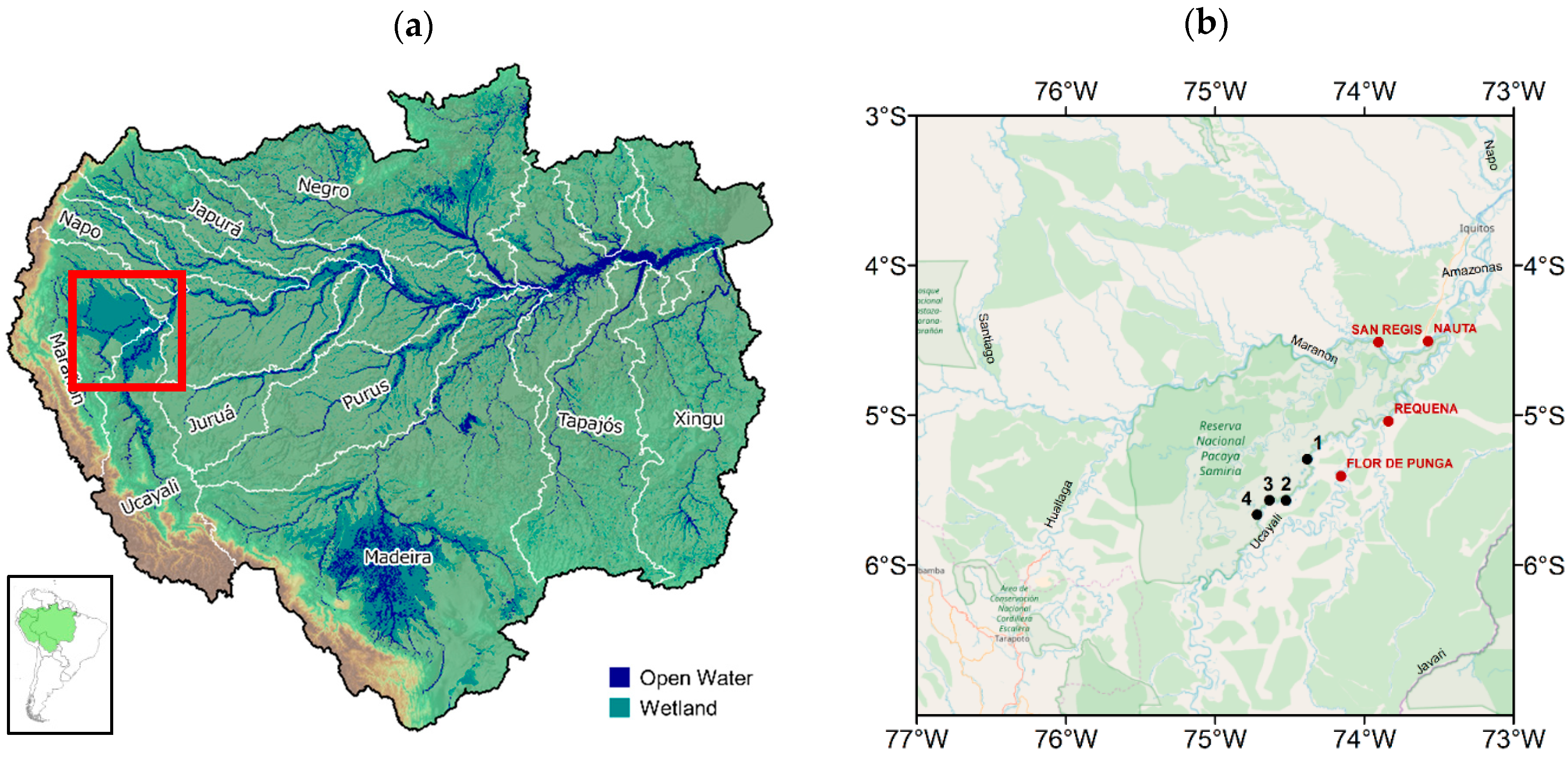
a) The Amazon Basin, illustrating primary river sub-basins and freshwater ecosystem extent, with the study region boxed in red. Data sources: open water and wetland delineation from Reference [
31]; sub-basin boundaries and GTOPO30 digital elevation model (DEM) from Reference [
32]; (
b) Extent of the study area, bounded by 3–7°S, 73–77°W, containing the Pacaya Samiria National Reserve. Locations of biometry measurement sites 1–4 along Canal de Puinahua are labelled in black. Field station location where river gauge data are available are shown in red.
Figure 1.
(
a) The Amazon Basin, illustrating primary river sub-basins and freshwater ecosystem extent, with the study region boxed in red. Data sources: open water and wetland delineation from Reference [
31]; sub-basin boundaries and GTOPO30 digital elevation model (DEM) from Reference [
32]; (
b) Extent of the study area, bounded by 3–7°S, 73–77°W, containing the Pacaya Samiria National Reserve. Locations of biometry measurement sites 1–4 along Canal de Puinahua are labelled in black. Field station location where river gauge data are available are shown in red.
Figure 2.
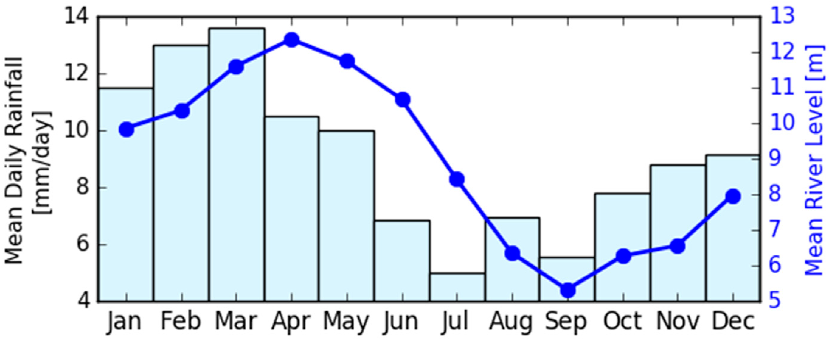
Mean monthly rainfall rate (mm/day) and mean monthly river level observed at Nauta field station (4°30′26.5″, 73°34′23.88″W), derived from daily observations over 2012–2017 provided by Servicio Nacional de Meteorologia e Hidrologia (Peru) [
33].
Figure 2.
Mean monthly rainfall rate (mm/day) and mean monthly river level observed at Nauta field station (4°30′26.5″, 73°34′23.88″W), derived from daily observations over 2012–2017 provided by Servicio Nacional de Meteorologia e Hidrologia (Peru) [
33].
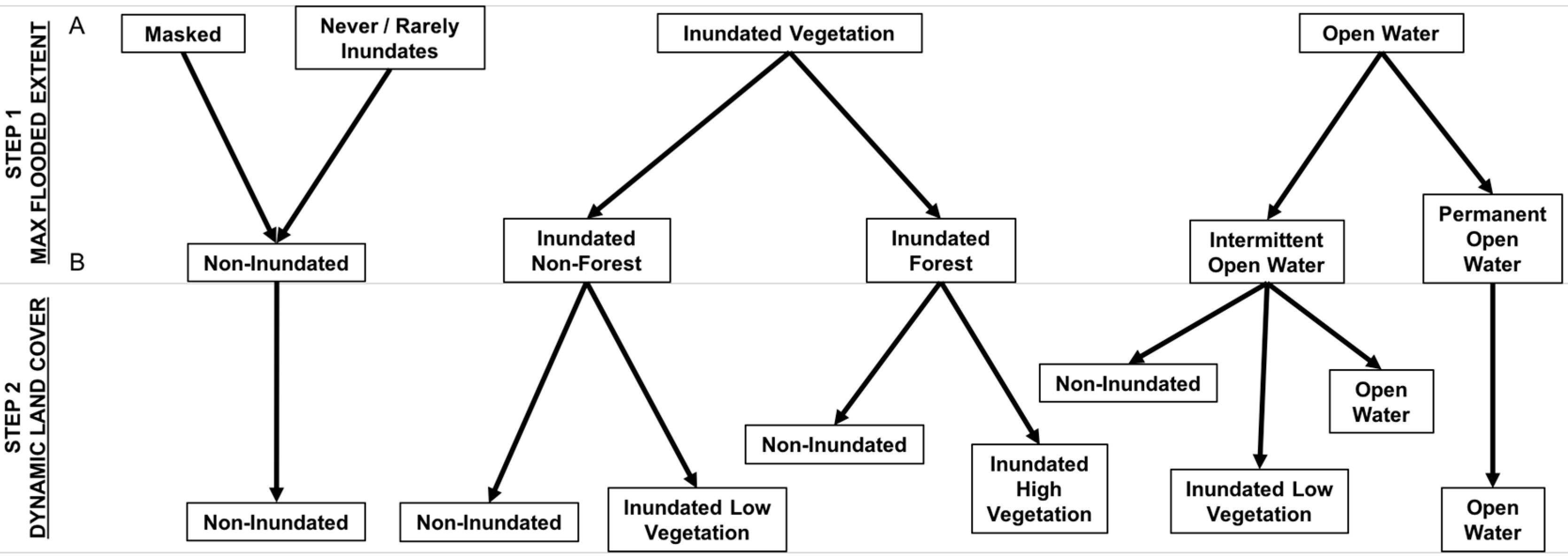
Figure 3.
Two-step classification scheme used to classify static maximum flooded extent and dynamic land cover types and flooding status. The decision tree was implemented with thresholds derived from ROIs corresponding to associated homogenous land cover classes.
Figure 3.
Two-step classification scheme used to classify static maximum flooded extent and dynamic land cover types and flooding status. The decision tree was implemented with thresholds derived from ROIs corresponding to associated homogenous land cover classes.
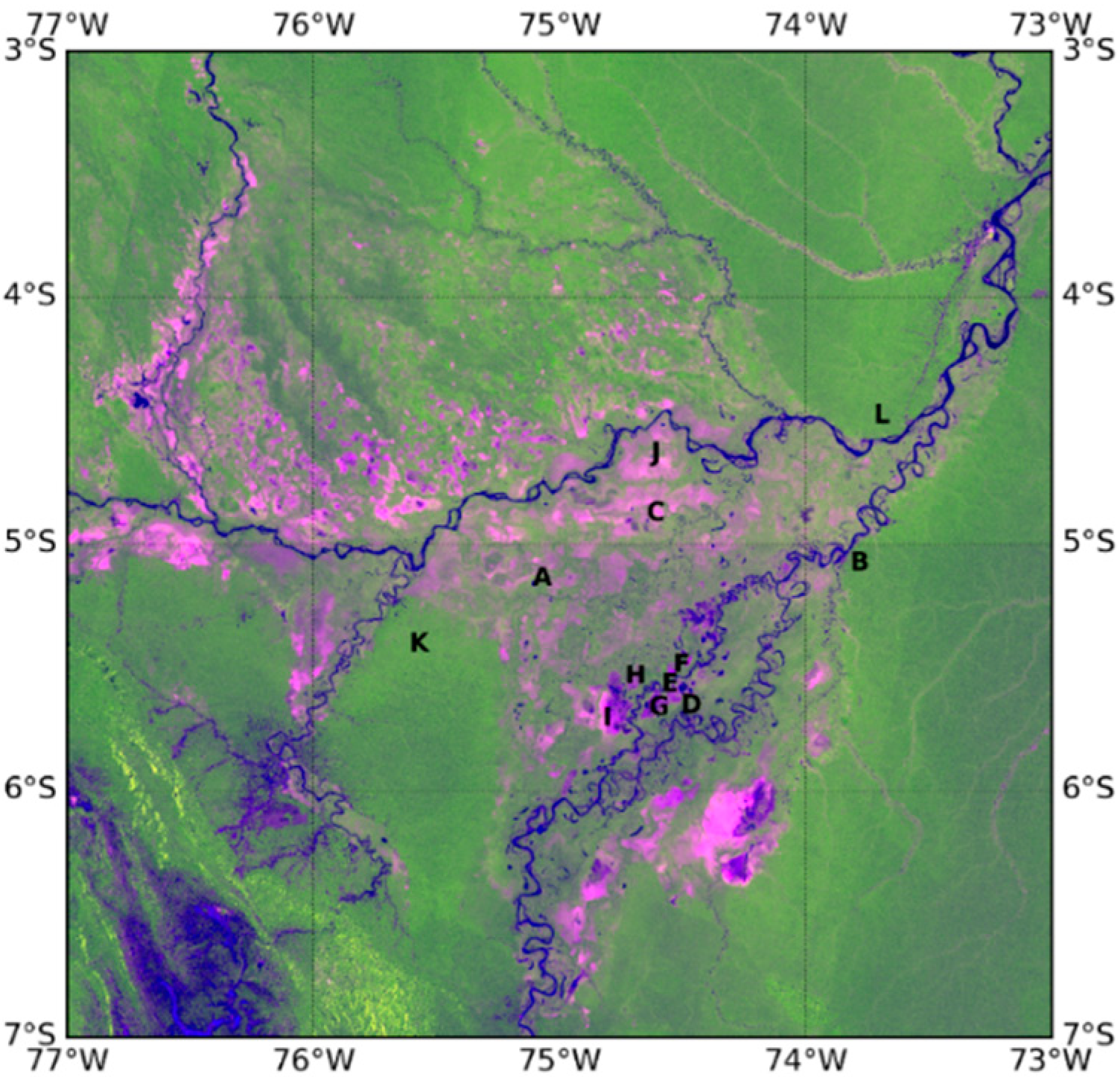
Figure 4.
False-color composite of temporal mean ALOS2 PALSAR-2 ScanSAR backscatter (Red: HH, Green: HV, Blue: HH/HV) with locations of ROIs.
Figure 4.
False-color composite of temporal mean ALOS2 PALSAR-2 ScanSAR backscatter (Red: HH, Green: HV, Blue: HH/HV) with locations of ROIs.
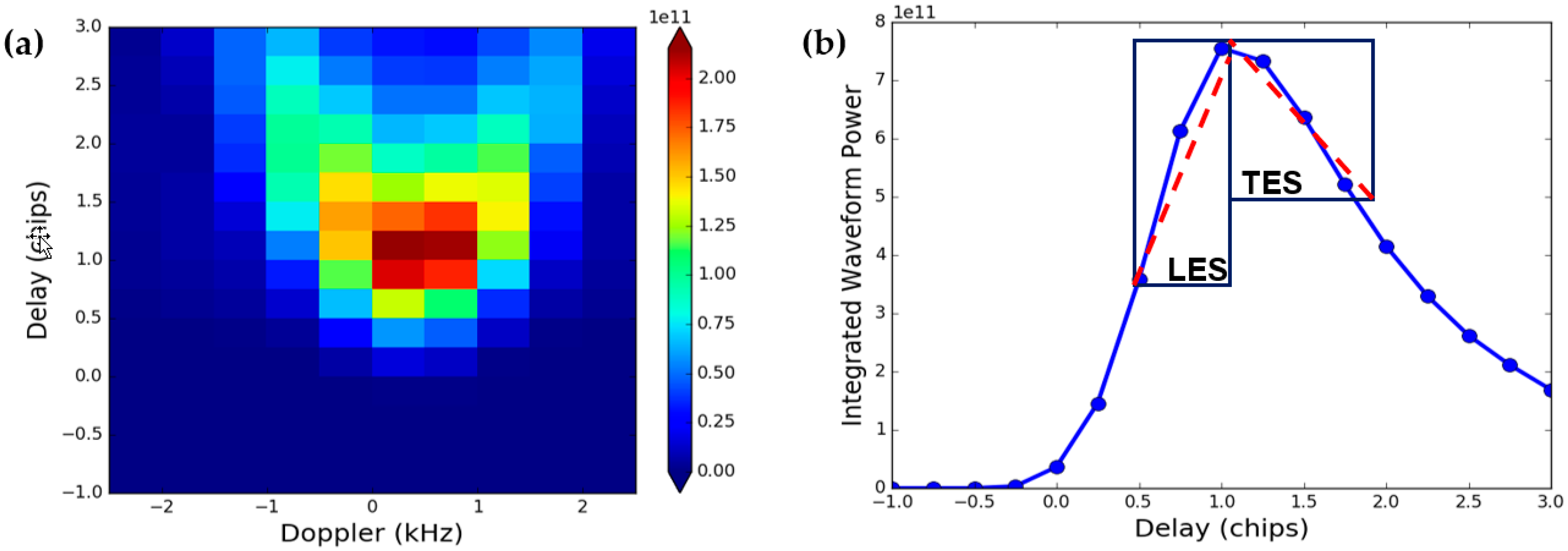
Figure 5.
(a) Example of a bistatic radar cross section Delay Doppler map (DDM); (b) integrated delay waveform (IDW) derived from (a). The leading edge slope (LES) is estimated from the peak in the IDW and the two preceding points, while trailing edge slope (TES) is derived from the IDW peak and three following points.
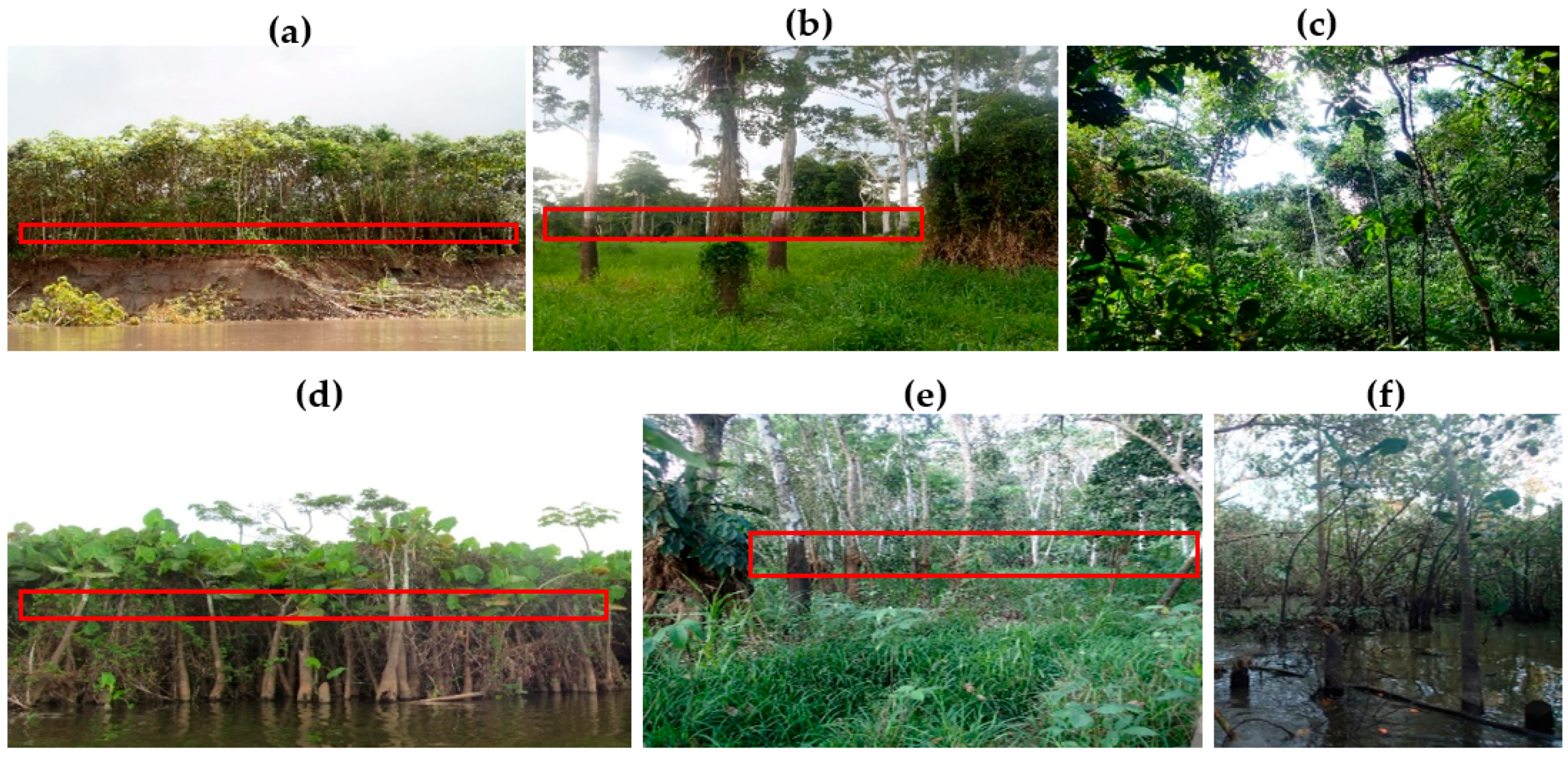
Figure 6.
Variety of floodplains observed at study sites (shown in
Figure 1b) in Pacaya Samiria at low water season. (
a) View of river bank near Site #1, (
b) open area in Site #1(in
Figure 1b) with sparse tree cover dominated by
Pseudobombax munguba; (
c) Dense canopy cover found in Site #2 (in
Figure 1b); (
d) inundated aquatic shrub species (
Montrichardia arborescens) found along margins of lake at Site #3(in
Figure 1b); (
e) denser tree cover and understory found in Site #3 (in
Figure 1b); (
f) inundated swamp found at Site #4 (in
Figure 1b). Examples of high flood marks on trees (shown red rectangles) indicate the level of previous inundation.
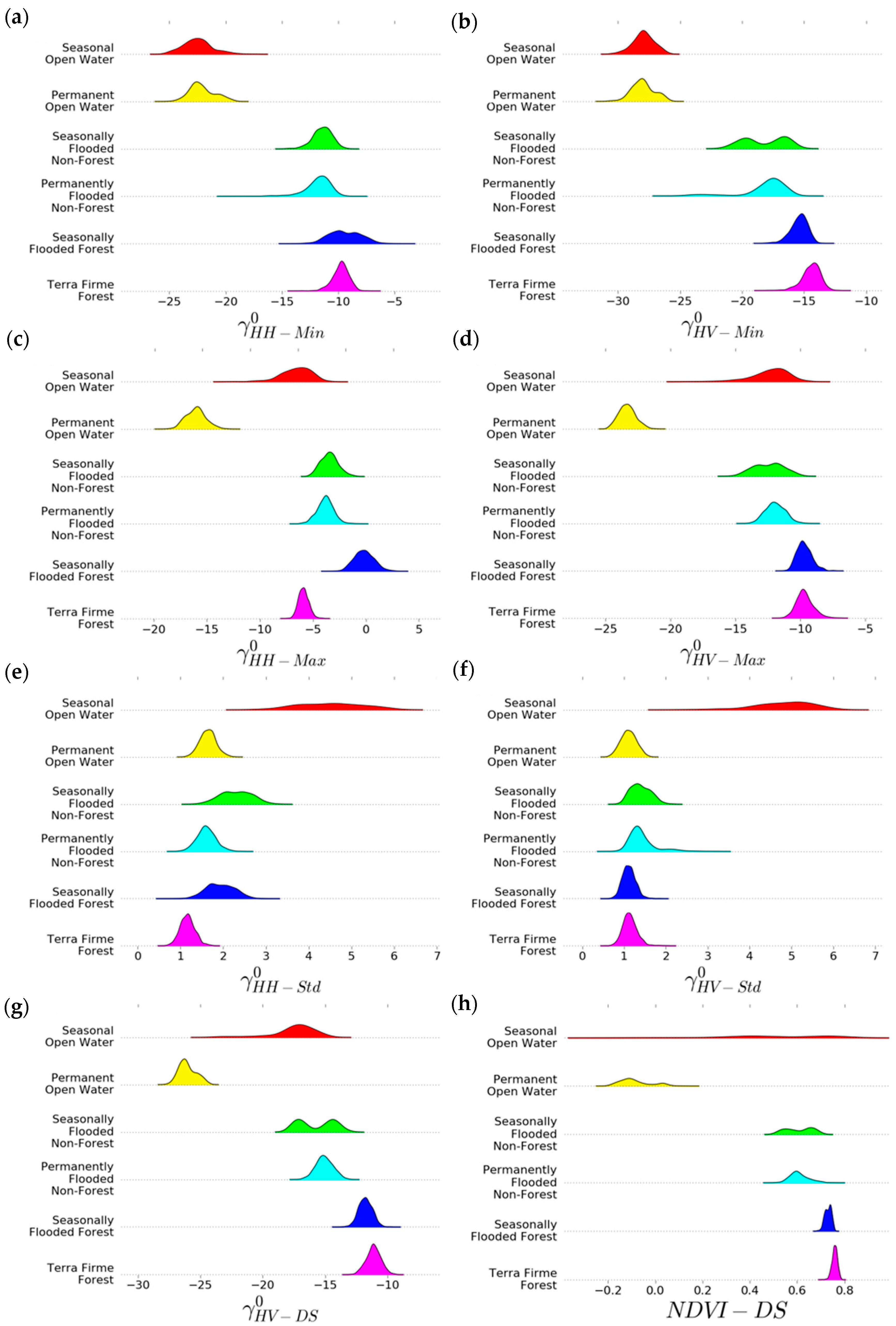
Figure 7.
Distribution of multi-temporal γ0 and NDVI statistics by land cover type from selected ROIs representing a variety of landcover classes: (a) , (b) , (c) , (d) , (e) , (f) , (g) , (h) NDVI-DS. Thresholding schemes for implementation of the decision tree classification are developed from these histograms.
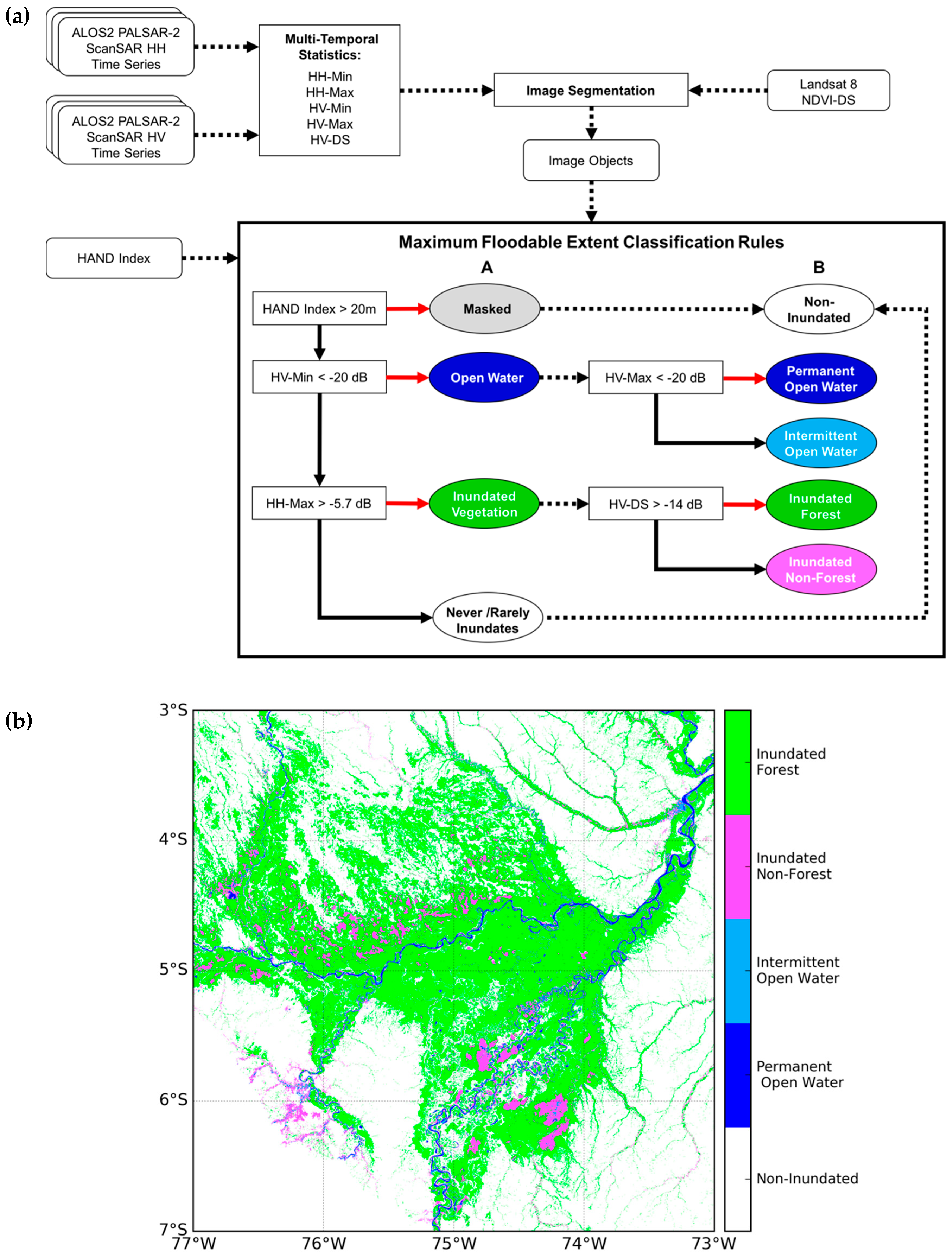
Figure 8.
(a) Step 1, object-based classification algorithm for maximum flooded extent. Boxes with rounded edges indicate inputs; boxes with sharp corners indicate a process/decision; ovals indicate assigned classes. In the decision tree, bold red arrows correspond with “True” and bold black arrows with “False”. (b) Maximum flooded extent classification map.
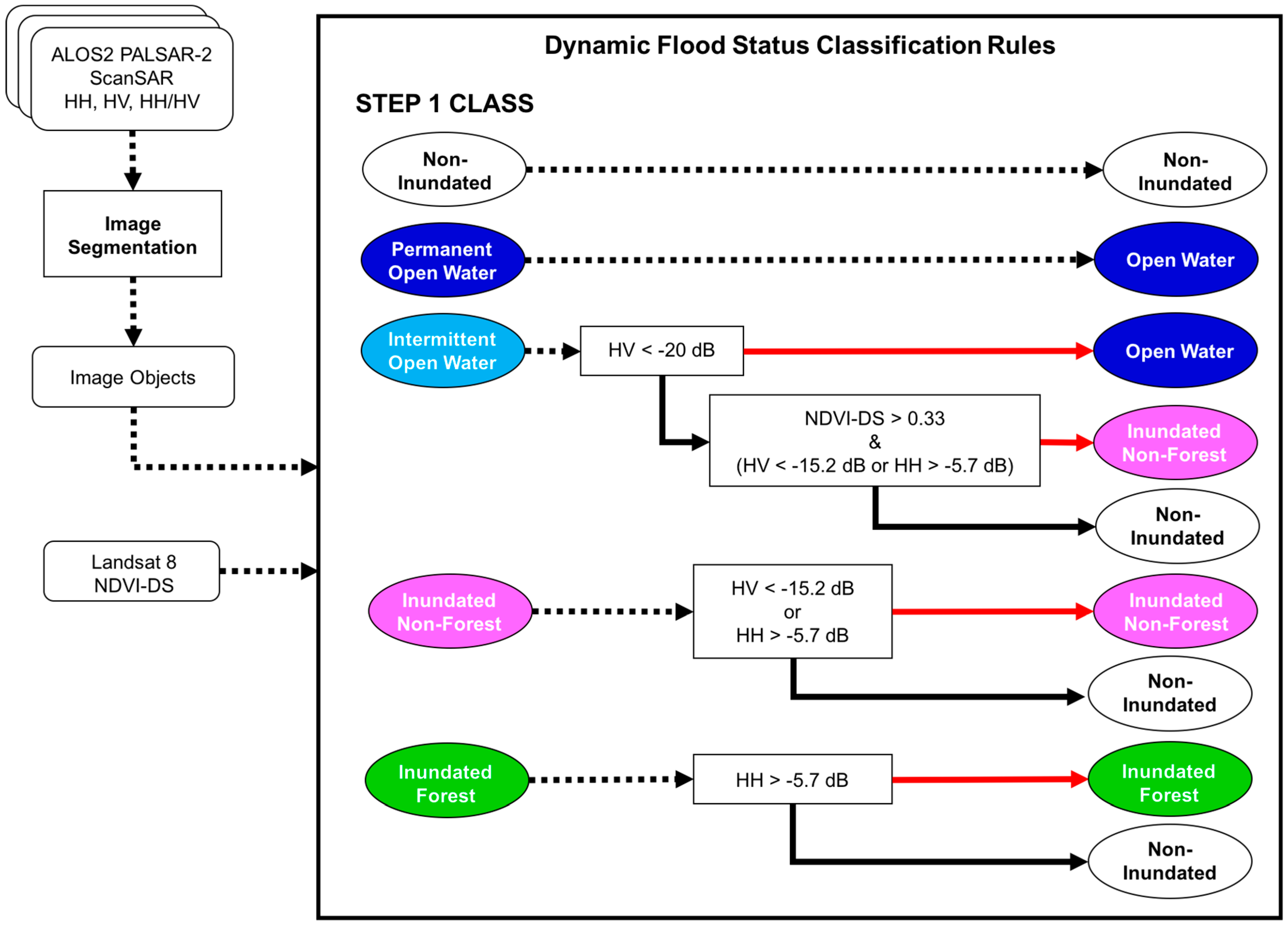
Figure 9.
Step 2 object-based classification algorithm for delineating time series inundation state. Boxes with rounded edges indicate inputs; boxes with sharp corners indicate a process/decision; ovals indicate assigned classes. In the decision tree, bold red arrows correspond with “True” and bold black arrows with “False”.
Figure 10.
Time series of PALSAR-2 classified flooded area percentage (open water, inundated non-forest and inundated forest) in the surrounding area within a 5 km radius and river level measurements (left) and scatter plots of corresponding values fitted to a logistic model (right) of the four field stations with locations shown in
Figure 1: (
a) Flor de Punga, (
b) Requena, (
c) Nauta, (
d) San Regis.
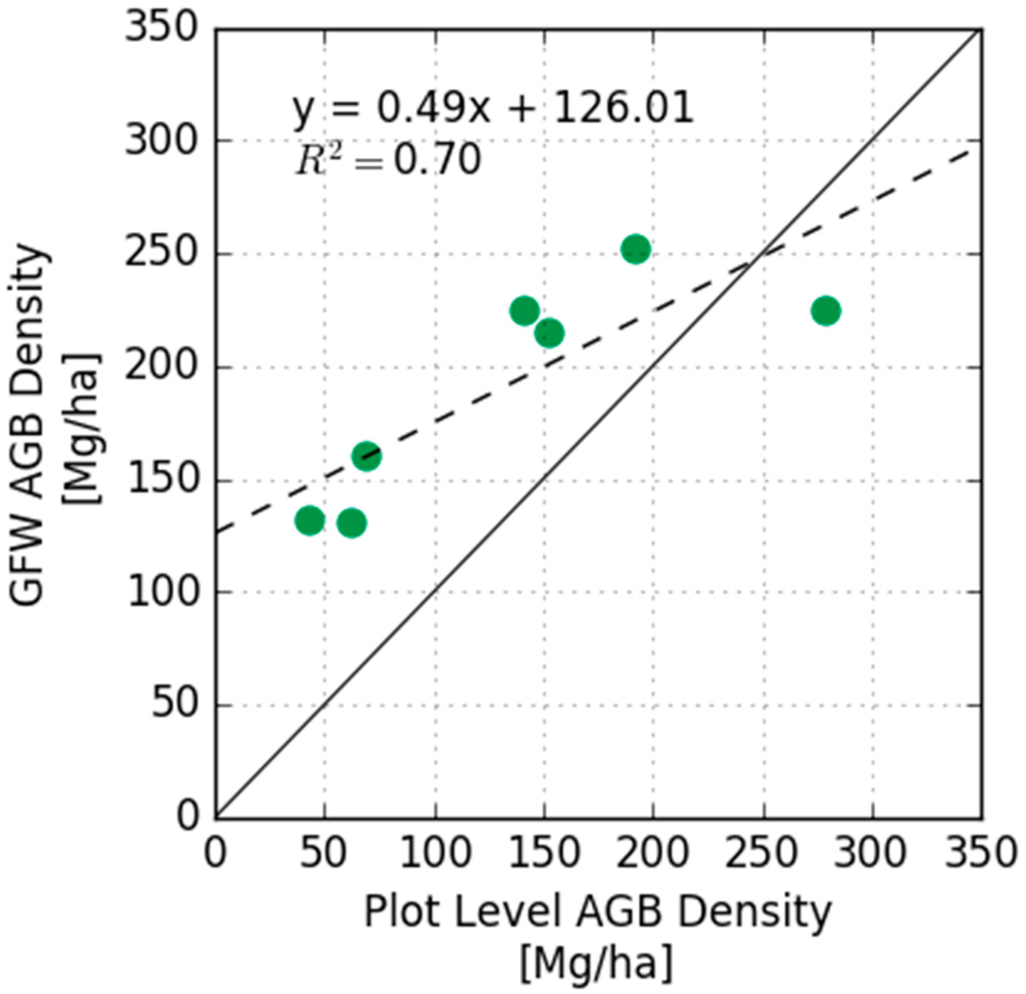
Figure 11.
Plot-level AGB density (x-axis) versus GFW-AGB density (y-axis). 1:1 line shown in solid black. Linear fit shown in dashed black, with equation and r-squared reported.
Figure 11.
Plot-level AGB density (x-axis) versus GFW-AGB density (y-axis). 1:1 line shown in solid black. Linear fit shown in dashed black, with equation and r-squared reported.
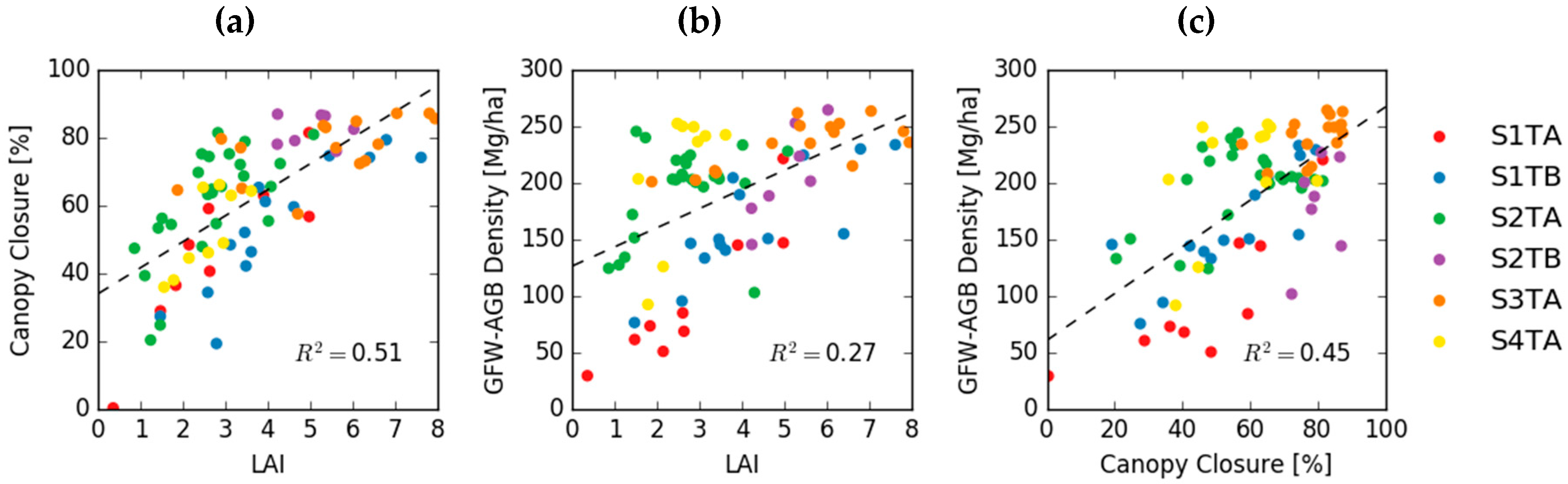
Figure 12.
(a) Relationship between LAI and canopy closure measured at transect points; (b) transect LAI (x-axis) versus GFW-AGB density (y-axis); (c) transect canopy closure (x-axis) versus GFW-AGB density (y-axis). Color of points corresponds to transect. Linear best-fit lines shown in dashed black, with r-squared values reported.
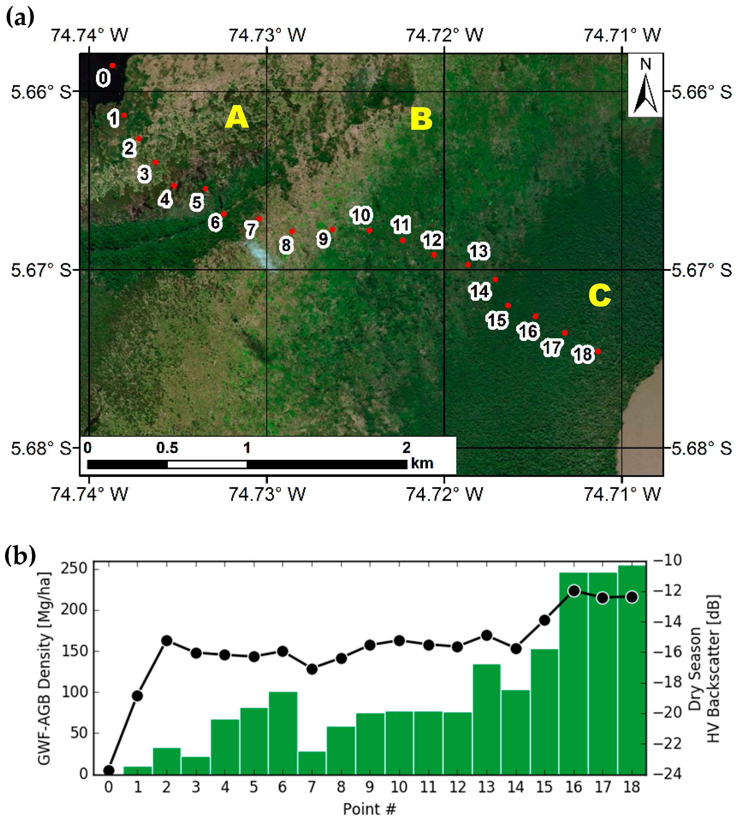
Figure 13.
(a) Transect through inundated swamp; (b) GFW-derived AGB density (green bar, left axis) and HV-polarized PALSAR-2 ScanSAR backscatter (black line, right axis) for each point shown in transect. Three 0.01° × 0.01° grid cells of interest are labelled A, B, C in yellow.
Figure 13.
(a) Transect through inundated swamp; (b) GFW-derived AGB density (green bar, left axis) and HV-polarized PALSAR-2 ScanSAR backscatter (black line, right axis) for each point shown in transect. Three 0.01° × 0.01° grid cells of interest are labelled A, B, C in yellow.
Figure 14.
CYGNSS footprint flooded area percentage estimated with classified PALSAR-2 mosaics vs. CYGNSS DDM observations, including SNR in top row (a–d), LES in center row (e–h), and TES in bottom row (i–l). Leftmost column displays all footprints, where % flooded counts flooded area regardless of vegetation (Open Water, Inundated Non-Forest, and Inundated Forest). The center left column presents the subset of the CYGNSS footprints with negligible inundated vegetation (Inundated Non-Forest and Inundated Forest of less than 5%), focusing only on the percentage of Open Water in each footprint. The center right column displays the subset of footprints with negligible Open Water (<1%) and displays the percentage of inundated vegetation (either Inundated Non-Forest or Inundated Forest). The rightmost column shows the subset of footprints with negligible Open Water or Inundated Non-Forest (<1%) and displays the percentage of Inundated Forest. Median values of DDM values are displayed in black, derived from bins of equal size (n = 1000).
![Remotesensing 10 01431 g014]()
Figure 15.
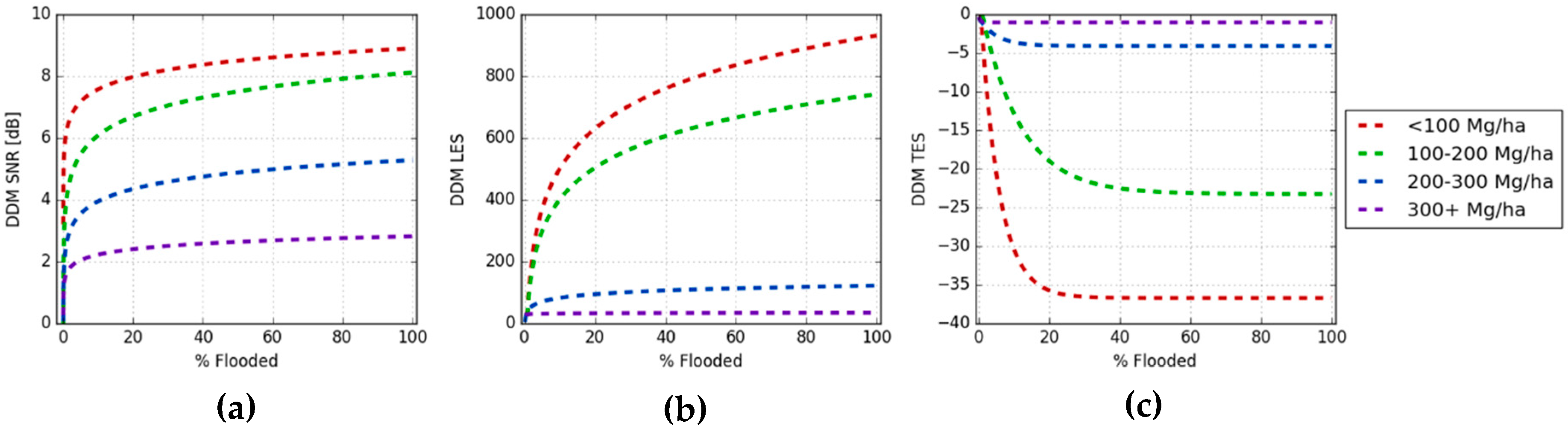
Relationship of footprint flooded area percentage (all flooded classes considered) vs. DDM (a) SNR; (b) LES; (c) TES. DDM observables are divided into four categories of GFW-AGB density (<100, 100–200, 200–300, and 300+ Mg ha−1), with best-fit logarithmic curves shown in (a,b) and exponential fit used in (c).
Figure 15.
Relationship of footprint flooded area percentage (all flooded classes considered) vs. DDM (a) SNR; (b) LES; (c) TES. DDM observables are divided into four categories of GFW-AGB density (<100, 100–200, 200–300, and 300+ Mg ha−1), with best-fit logarithmic curves shown in (a,b) and exponential fit used in (c).
Figure 16.
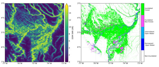
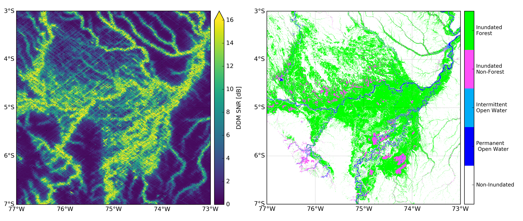
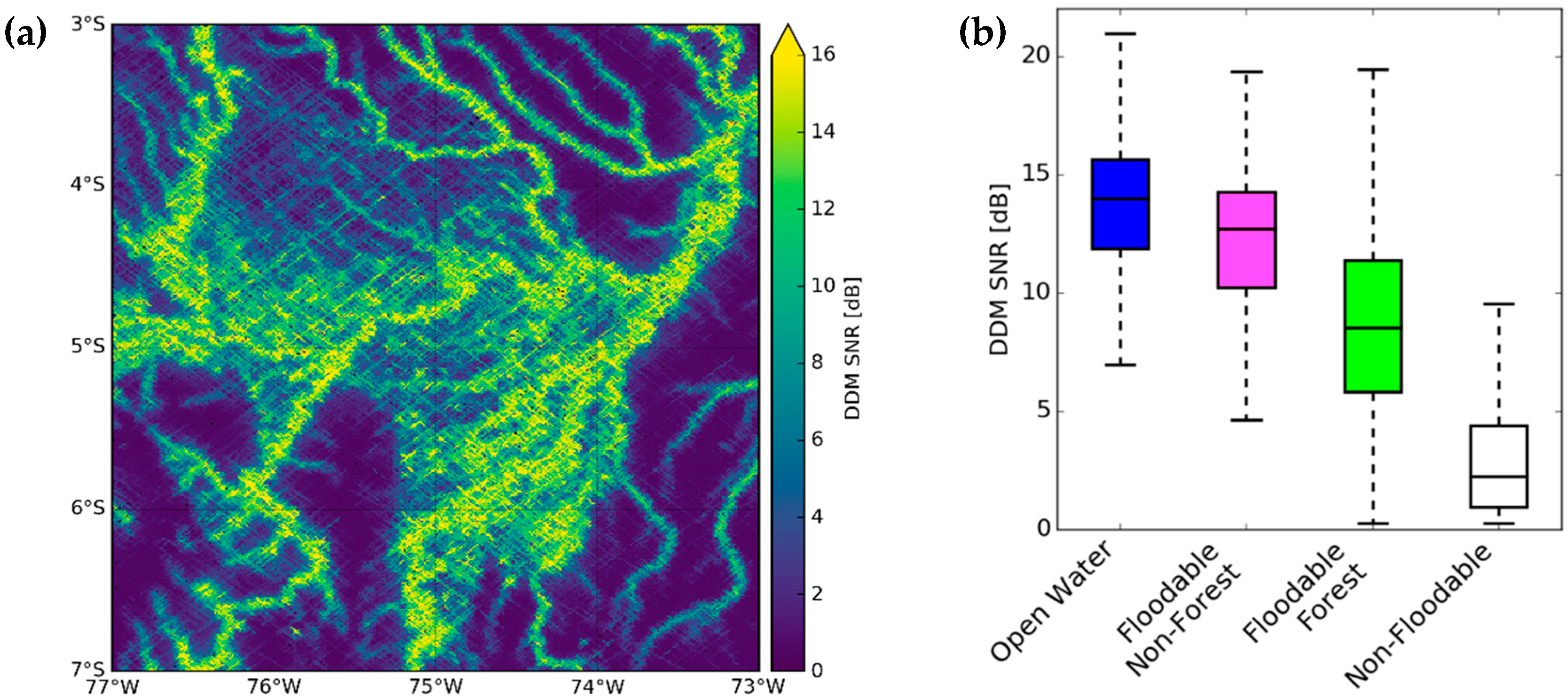
(a) Maximum CYGNSS DDM SNR observed between 18 March 2017–15 February 2018, posted at 0.01° (~1 km) grid; (b) box plot delineating maximum DDM SNR grouped by PALSAR-2 maximum flooded extent class, including only 1 km pixels that are dominantly one class (≥99%). Central rectangle spans the first quartile to the third quartile (interquartile range), with median value illustrated as line inside the rectangle, and the minimum and maximum values indicated by the extent of the whiskers above and below the box.
Figure 16.
(a) Maximum CYGNSS DDM SNR observed between 18 March 2017–15 February 2018, posted at 0.01° (~1 km) grid; (b) box plot delineating maximum DDM SNR grouped by PALSAR-2 maximum flooded extent class, including only 1 km pixels that are dominantly one class (≥99%). Central rectangle spans the first quartile to the third quartile (interquartile range), with median value illustrated as line inside the rectangle, and the minimum and maximum values indicated by the extent of the whiskers above and below the box.
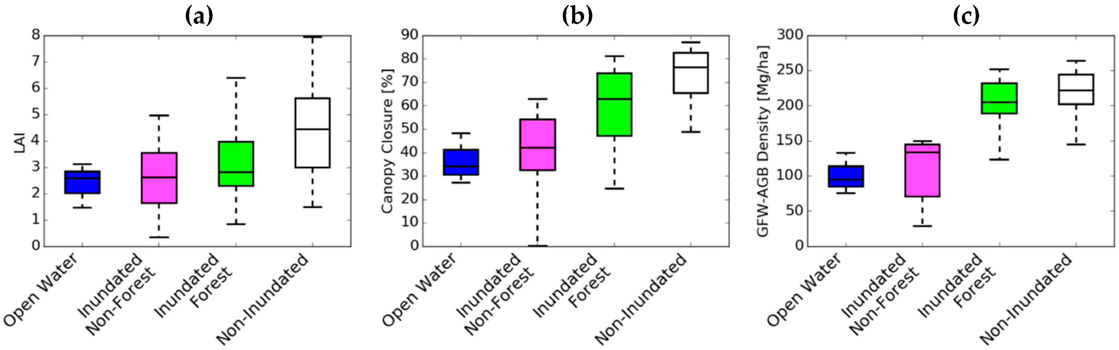
Figure 17.
Distribution of vegetation structure metrics of transect points that showed evidence of seasonal flooding, grouped by PALSAR-2 maximum flooded extent class: (a) LAI; (b) canopy closure; (c) GFW-AGB density.
Figure 17.
Distribution of vegetation structure metrics of transect points that showed evidence of seasonal flooding, grouped by PALSAR-2 maximum flooded extent class: (a) LAI; (b) canopy closure; (c) GFW-AGB density.
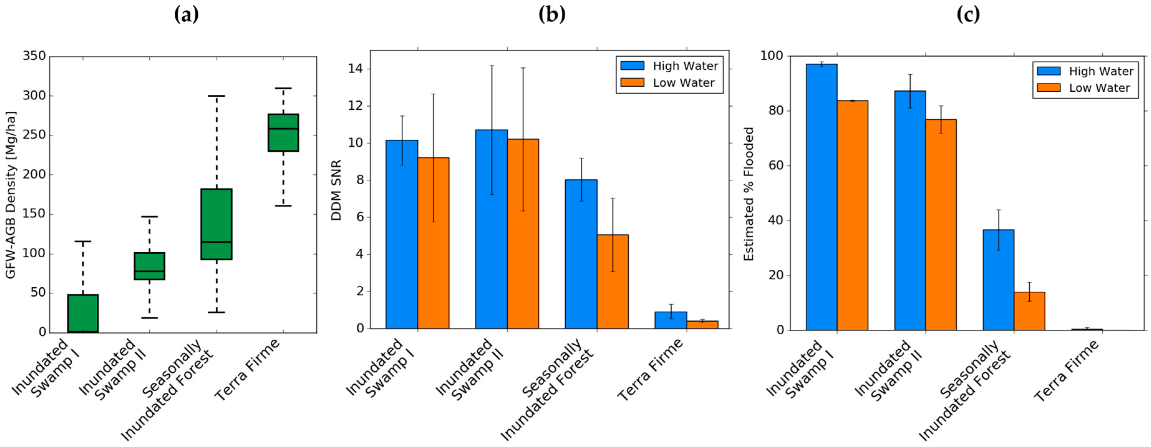
Figure 18.
Comparison of high vs. low water seasons in 2017 at four 0.01° grid cells. (a) Distribution of estimated GFW-AGB density observed in each grid cell; (b) observed CYGNSS DDM SNR during high vs. low water seasons in each region (number of observations ranged from 3–8 per season for each region); (c) estimated flooded area percentages derived from PALSAR-2 during high vs. low water seasons in each region (number of observations was 2 or 3 per season for each region). Bar charts (b,c) show mean values observed in seasonal window, with standard deviation indicated by error bars.
Table 1.
Characteristics of selected ROIs and descriptive summaries of dry season NDVI and multi-temporal γ0 statistics observed.
Table 1.
Characteristics of selected ROIs and descriptive summaries of dry season NDVI and multi-temporal γ0 statistics observed.
| ROI | Land Cover | Size(#Pixels) | NDVI-DS | | | | |
|---|
| A | Seasonal Open Water | 307 | 0.37 | −11.4 | −18.3 | 4.8 | 4.9 |
| B | Seasonal Open Water | 312 | 0.50 | −11.7 | −18.5 | 4.1 | 4.5 |
| C | Permanent Open Water | 443 | 0.01 | −18.3 | −24.8 | 1.6 | 0.9 |
| D | Permanent Open Water | 1307 | −0.11 | −19.4 | −25.9 | 1.6 | 1.2 |
| E | Seasonally Flooded NF | 516 | 0.65 | −5.5 | −14.2 | 2.1 | 1.3 |
| F | Seasonally Flooded NF | 470 | 0.54 | −5.4 | −16.7 | 2.5 | 1.5 |
| G | Permanent Flooded NF | 1323 | 0.58 | −6.3 | −14.8 | 1.5 | 1.3 |
| H | Permanent Flooded NF | 279 | 0.57 | −6.7 | −15.7 | 1.6 | 1.1 |
| I | Seasonally Flooded Forest | 1957 | 0.74 | −2.6 | −13.0 | 2.0 | 1.1 |
| J | Seasonally Flooded Forest | 1576 | 0.72 | −4.1 | −12.9 | 2.2 | 1.1 |
| K | Terra Firme Forest | 1807 | 0.76 | −7.3 | −11.9 | 1.2 | 1.1 |
| L | Terra Firme Forest | 472 | 0.75 | −7.2 | −12.6 | 1.4 | 1.2 |
Table 2.
Accuracy assessment of Step 1 maximum flooded extent classification compared with IIAP reference map of Pacaya Samiria National Reserve.
Table 2.
Accuracy assessment of Step 1 maximum flooded extent classification compared with IIAP reference map of Pacaya Samiria National Reserve.
| IIAP Reference |
|---|
| PALSAR-2 Maximum Extent | | Open Water | Inundated Non-Forest | Inundated Forest | Non-Inundated | Total | User’s Accuracy | Commission Error |
| Open Water | 38,860 | 3617 | 23 | 3 | 42,503 | 91.4% | 8.6% |
| Inundated Non-Forest | 2798 | 275,685 | 13,571 | 167 | 292,221 | 94.3% | 5.7% |
| Inundated Forest | 657 | 17,485 | 3,006,949 | 19,282 | 3,044,373 | 98.8% | 1.2% |
| Non-Inundated | 33 | 6579 | 363,945 | 1,468,284 | 1,838,841 | 79.8% | 20.2% |
| Total | 42,348 | 303,366 | 3,434,488 | 1,487,736 | 5,217,938 | | |
| Producer’s Accuracy | 91.8% | 90.9% | 88.8% | 98.7% | | | |
| Omission Error | 8.2% | 9.1% | 11.2% | 1.3% | | | |

 ,
, 


