Article

Remote Sensing of Leaf and Canopy Nitrogen Status in Winter Wheat (Triticum aestivum L.) Based on N-PROSAIL Model

1
Beijing Research Center for Information Technology in Agriculture, Beijing Academy of Agriculture and Forestry Sciences, Beijing 100097, China
2
National Engineering Research Center for Information Technology in Agriculture, Beijing 100097, China
3
School of Engineering, Newcastle University, Newcastle upon Tyne NE1 7RU, UK
4
UMR EMMAH, INRA, NAPV, 84914 Avignon, France
5
School of Geographical and Earth Sciences, University of Glasgow, Glasgow G12 8QQ, UK
6
School of Natural and Environmental Sciences, Newcastle University, Newcastle upon Tyne NE1 7RU, UK
*
Authors to whom correspondence should be addressed.
Submission received: 26 June 2018 / Revised: 6 September 2018 / Accepted: 10 September 2018 / Published: 13 September 2018
(This article belongs to the Special Issue Remote Sensing for Precision Nitrogen Management)

Abstract

:
Plant nitrogen (N) information has widely been estimated through empirical techniques using hyperspectral data. However, the physical model inversion approach on N spectral response has seldom developed and remains a challenge. In this study, an N-PROSAIL model based on the N-based PROSPECT model and the SAIL model canopy model was constructed and used for retrieving crop N status both at leaf and canopy scales. The results show that the third parameter (3rd-par) retrieving strategy (leaf area index (LAI) and leaf N density (LND) optimized where other parameters in the N-PROSAIL model are set at different values at each growth stage) exhibited the highest accuracy for LAI and LND estimation, which resulted in R2 and RMSE values of 0.80 and 0.69, and 0.46 and 21.18 µg·cm−2, respectively. It also showed good results with R2 and RMSE values of 0.75 and 0.38% for leaf N concentration (LNC) and 0.82 and 0.95 g·m−2 for canopy N density (CND), respectively. The N-PROSAIL model retrieving method performed better than the vegetation index regression model (LNC: RMSE = 0.48 − 0.64%; CND: RMSE = 1.26 − 1.78 g·m−2). This study indicates the potential of using the N-PROSAIL model for crop N diagnosis on leaf and canopy scales in wheat.

Graphical Abstract

1. Introduction

Nitrogen (N) is a critical nutrient element for maintaining photosynthesis, enhancing production, and improving grain quality in crops, but the excess use of N fertilizer also results in a series of plant and environmental problems (e.g., vigorous growth, and eutrophication) [1,2]. Precision farming, which considers the crop spatial N distribution, plays an important role in solving these problems, whereby the accurate crop N estimation by remote sensing technology has the potential to precisely manage N by supplying a crop’s N requirement at the right place and right time [3,4].
Various sensitive spectral features and vegetation indices have been analyzed for crop N estimation. Kokaly proposed that leaf N concentration (LNC, %) in rice can be estimated by two reflectance absorptions at 2054 nm and 2172 nm [5]. Niu et al. showed that fresh LNC could be estimated using first derivative reflectance spectrum at 2120 nm and 1120 nm [6]. Cho and Skidmore reported on extracting two optimal red edge region equations (REP = − (c1c2)/(m1m2), where c1 and c2 are the intercepts of a far-red line connected between 679.65 and 694.30 nm, and near-infrared line connected between 732.46 and 760.41 nm or 723.64 and 760.41 nm, respectively; m1 and m2 are the corresponding slope of c1 and c2, respectively) with high N sensitivity [7]. Previous studies demonstrated that spectral indices have a high correlation with crop N status [8,9,10,11,12,13,14,15,16], and many spectral indices centered on crop N were proposed. Normalized Difference N Index (NDNI = [log(1/R1510) − log(1/R1680)]/[log(1/R1510) + log(1/R1680)] was used to estimate LNC in native shrub vegetation [9]. Elshikha et al. presented the Canopy Chlorophyll Content Index [CCCI = (NDRE − NDREmin)/(NDREmax − NDREmin), where NDRE = (R790R720)/(R790 + R720)] as an effective indicator to monitor cotton N when the canopy cover reached above 30% [17]. Yao et al. found the model for canopy N density (CND, g·m-2) estimation based on NDSI (R860, R720), RSI (R990, R720), NDSI (FD736, FD720), and RSI (FD725, FD516) performed well in wheat [15]. Chen et al. developed a new index named Double-peak Canopy N Index [DCNI = (R720R700)/(R700R670)/(R720R670 + 0.03)] to estimate plant N concentration (PNC) in corn and wheat [13]. Feng et al. created a Water Resistance N Index [WRNI = (R735R720) × R900/Rmin(930-980)/(R735 + R720)] to improve the accuracy of the LNC model by minimizing water effects at different growth stages [16].
Moreover, the application of artificial intelligence methods in crop N estimation has been reported in many recent studies and has been proved to be a better predictor than using only sensitive spectral features or vegetation indices [3,4,18,19,20,21,22,23,24]. Among these, Hansen et al., Ecarnot et al., and Li et al. showed that partial least square regression (PLSR) could accurately predict LNC in winter wheat and winter oilseed rape [18,19,20]. Miphokasap et al. indicated that estimaing PNC by stepwise multiple linear regression (SMLR) performed a higher estimation than the model by vegetation indices [4]. Zhang et al. demonstrated that an artificial neural network (ANN) improved the prediction of LNC with consistently higher R2 values, and was better than that by SMLR [21]. Xu et al. proposed that the optimal combination principle (OCP) method to monitor LNC in barley would exhibit better performance than the vegetation indices methods [22,23]. Yao et al. and Li et al. compared the method of SMLR, PLSR, ANN, and support vector machines regression (SVR), to monitor LNC, and showed PLSR and SVR to be preferred choices for estimating LNC, and ANN was also recommended when sufficient sample size was available [1,24].
Much research on crop N estimation has been reported, and some results were satisfactory. However, a statistical relationship between spectral information and crop N status cannot be expected everywhere and every time, even for a particular sensor [25,26]. The physical model inversion approach on N spectral response has rarely been developed, except for an N-based PROSPECT model (N-PROSPECT) which was extended from a PROSPECT model by replacing the specific absorption coefficients of chlorophyll in the model with equivalent N absorption coefficients, and which could accurately simulate and retrieve leaf N density (LND) at the leaf scale [27]. Thus, crop N status both at leaf and canopy scales could be retrieved through integrating the N-PROSPECT model and the SAIL canopy model [28], to be defined as the N-PROSAIL model in this study. In addition, an ill-posed problem, also called inaccurate inversion, existed and is unavoidable in model parameters inversion, which could be attributed to: (1) multiple solutions in the process of the inversion and (2) uncertainties from measurements and model assumptions [25,26]. Using prior information has been demonstrated as a very efficient solution to this problem [29,30].
To develop an N estimation model based on physical model and explore the suitable strategies for estimating leaf and canopy N status, the objectives of this research were: (1) to develop the N-PROSAIL model to simulate canopy reflectance responses to leaf N density (LND); (2) to assess N status both at leaf and canopy scales, i.e., LNC and canopy N density (CND, g·m−2 soil), in winter wheat using the N-PROSAIL model; (3) to reduce the ill-posed inversion and improve the accuracy of related N variables by setting prior parameters values in the N-PROSAIL model at different growth stages; and (4) to evaluate the performance of the N-PROSAIL model method by comparing it with LNC and CND estimated by vegetation index methods.

2. Materials and Methods

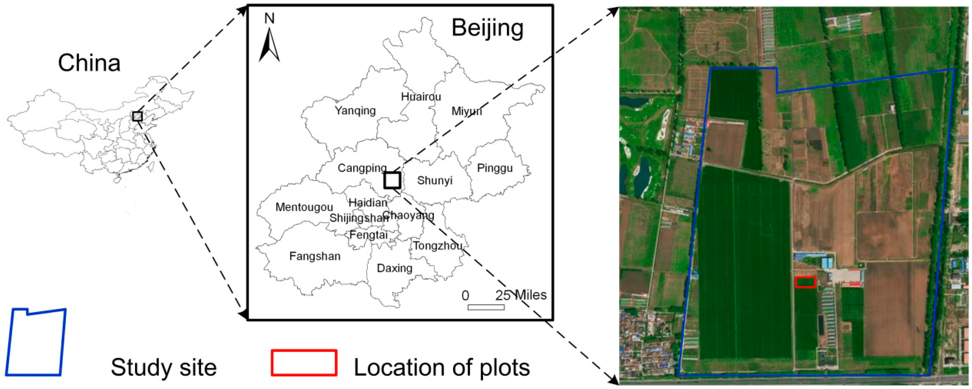
2.1. Experimental Design

The experiments were conducted over four growing seasons, 2012–2013, 2013–2014, 2014–2015, and 2015–2016, at the Xiaotangshan National Experimental Station for Precision Agriculture, (40.17°N, 116.43°E) in Beijing, China (Figure 1). The test variables included various cultivars, different N fertilization rates and irrigation amounts (Table 1). Experiment (Exp.) 1 was carried out in 2012–2013 as a completely randomized design with two replications of four wheat cultivars and four N fertilizer applications rates. Exp. 2 and 3 were conducted in 2013–2015 with an orthogonal experimental design with three replications of two wheat cultivars, four N fertilizer applications rates, and three irrigation amounts. Exp. 4 was designed in 2015–2016 as a completely randomized design with three replications of two wheat cultivars and four N fertilizer applications rates. Other management procedures such as pest management, weed control, and phosphate and potassium fertilizer followed local standard practices for winter wheat production.

2.2. Data Acquisition

2.2.1. Canopy Spectral Data

Canopy hyperspectral reflectances were obtained at four key growth stages (Zadoks growth stage: 31, 47, 65, 75 of winter wheat) [31] (Table 2). Canopy reflectances were measured by an ASD FieldSpec Handheld spectrometer (Analytical Spectral Devices Inc., USA) with a spectral range of 350–2500 nm. Under clear sky conditions between 10:00 and 14:00 Beijing time, the spectrometer was held at a height of 1.0 m above the canopy to ensure the same corresponding at different growth stages. A 40 cm by 40 cm BaSO4 calibration panel served as a black, baseline reflectance. To reduce the possible effects of sky and field conditions, spectral measurements were taken at four sites in each plot and then averaged to represent the canopy reflectance of each plot. Vegetation and panel radiance measurements were taken as the average of 20 scans at an optimized integration time, with a dark current correction for each spectrometry measurement. A panel radiance measurement was taken before and after each vegetation measurement by two scans. Bare soil refelectance was also acquired at each growth period so that it could be used as the input of the N-PROSAIL model.

2.2.2. Plant Measurements

The aboveground vegetation at spectral measurement positions was collected immediately by randomly cutting 0.25 m2 in each plot, and the number of tillers counted. Then, plant samples of 20 representative wheat tillers were randomly selected from the collected cut plants. All green leaves were separated from the stems. A laser leaf area meter (CI-203, CID Bio-Science Inc., WA, USA) was used to measure the leaf area, and electronic scales (±0.01 g) and drying oven were used to get the leaf dry mass, wet matter weight and dry matter weight (Cm, g·m−2) [26]. Equivalent water thickness (Cw, g·cm−2 or cm) was calculated based on wet matter weight and dry matter weight [32]. A Carlo-Erba NA 1500 dry combustion analyzer (Carlo Erba, Milan, Italy) [33] was used to measure leaf N concentration (LNC, %). Finally, leaf N density (LND, µg·cm−2 leaves) was calculated as the LNC multiplied by the Cm, and canopy N density (CND, g·m−2 soil) was acquired by leaf area index (LAI) multiplied by LND [27,34].

2.3. Model and Methods

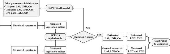
2.3.1. Inversion Procedure of LNC and CND Estimation

The inversion procedure of LNC and CND estimation with the N-PROSAIL model is shown in Figure 2. Specific steps were as follows:
(1) Prior parameters initialization: parameters in the N-PROSAIL model (see Section 2.3.2) were initialized and simulated references can be simulated based on these set parameters. Three strategies of parameter (par) setting were tested and are as follows:
(i)
1st-par: LAI, LND and Cm were optimized and the other six parameters in the N-PROSAIL model (Table 3) were set as fixed values in the whole growth period;
(ii)
2nd-par: LAI, LND and Cm were optimized and the other six parameters in the N-PROSAIL model (Table 3) were set as fixed values at each growth stage;
(iii)
3rd-par: LAI and LND were optimized and Cm was also set as fixed values at each growth stage since it has low variation in specific crop cultivar at one growth stage [35,36]. The other six parameters in the N-PROSAIL model were set as 2nd-par.
(2) Vegetation indices calculation: simulated and measured vegetation indices (see Section 2.3.3) were computed and the optimal vegetation indices correlative with LAI, LND and Cm were chosen to construct cost function in optimization method.
(3) SCE-UA optimization: the SCE-UA method (see Section 2.3.4) was used to optimize parameters in the N-PROSAIL model. Parameters of the SCE-UA method were set and parameters in the N-PROSAIL model were updated until the number of optimization iterations was more than the maximum number of trials (maxn) allowed before optimization was terminated.
(4) Validation: the end LAI, LND and Cm were considered as optimized values and they were used to calculate LNC and CND. Three strategies were validated by comparing measured and simulated values. In addition, the inversion performance by the N-PROSAIL model was compared with LNC and CND estimation modeled by vegetation indices.

2.3.2. The N-PROSAIL Model

The N-PROSAIL model is a combination of the N-PROSPECT leaf model [27] and SAILH canopy model [28]. At the leaf scale, PROSPECT uses a leaf structure parameter and leaf biochemical contents to simulate directional-hemispherical reflectance and transmittance of various leaves [37]. The N-PROSPECT model was developed from the PROSPECT model by replacing the specific absorption coefficients of chlorophyll in the PROSPECT model with equivalent N absorption coefficients [27,37]. LNC can be estimated according to LND and Cm. At canopy scale, SAILH considers canopy structures (LAI, leaf angle distribution (θs)), soil brightness, and other angle information to generate canopy reflectance [28]. LAI can be retrieved according to the SAIL model. Then, CND can be calculated by multiplying LAI and LND. During the inversion of the N-PROSAIL model to retrieve crop parameters, nine parameters needed to be determined (Table 3). These parameters were determined at different growth stages. LAI and LND were the main retrieval parameters and they were given intervals based on calibration dataset. Cw, Cm and Soil brightness parameter (Rsoil) values were obtained by averaging measured values at different growth stages. The solar zenith angle (θs) was calculated for the time in the experiment when the hyperspectral data was measured. Leaf structure parameter (Ns), hot spot parameter (SL) and leaf inclination distribution (LID) values were firstly optimized by the SCE-UA method using the 2012–2013, 2013–2014 and 2015–2016 wheat experiment data, where parameters of LAI, LND, Cw, Cm, Rsoil, θs were known inputs. Then the mean values of Ns, LID at different growth stages were the final results. Finally, we got the parameter set of Cw, Cm, Rsoil, θs, Ns, SL and LID at each growth stage, respectively (Table 3).

2.3.3. Selection of Spectral Index

Fifteen vegetation indices correlated with agronomic parameters in previous results were calculated using the equations listed in Table 4. Using these vegetation indices has the following two purposes. (1) Selecting the best vegetation index correlation with LAI, LND and Cm to establish the cost function, an equation to evaluate the consistency between simulated and measured target, in the N-PROSAIL model (see Section 2.3.4). (2) Establishing regression equations of LNC and CND, which were used to validate the inversion performance using the N-PROSAIL model.

2.3.4. SCE-UA Algorithm for LNC and CND Estimation

The SCE-UA method (the abbreviation for the Shuffled Complex Evolution method developed at the University of Arizona) proposed by Duan et al. is a general purpose global optimization program [50]. The method has the advantages of search efficiency at high-parameter dimensionality, convergence speed and computational efficiency, and global searching stability [51,52], and it has been proved to be a useful and effective optimization method in past studies [53,54,55]. Duan et al. [51] and Wang et al. [54] give a detailed description of the steps of the SCE-UA method. There are many parameters in the SCE-UA method, but most of them were set as default in the method. The number of complexes in a sample population (ngs) and the maximum number of trials (maxn) were determined by the actual condition and they are 2 and 1000 in this study, respectively [54]. The cost function used to compare simulated with measured vegetation indices in this study was selected as follows:
J = i = 1 N ( V Im i V I s i ) 2 V Im i  
where J is the value of cost function and N is the determined number of vegetation indices. VIm and VIs are the measured vegetation indices and simulated vegetation indices by the N-PROSAIL model, respectively. In this study, three vegetation indices respectively correlated with LAI, LND, and Cm, were selected into the cost function. In the process of iterative inversion, the minimum of J value (minJ) was given as 5% to avoid model overfitting. Thus, the terminal condition happens when the iterative number is larger than maxn or the J value is less than minJ.

2.3.5. Statistical Analysis

Data collected from 2012–2013, 2013–2014, and 2015–2016 (n = 384) were mainly used for analyzing the correlation between vegetation indices and agronomic variables, calibrating the parameters of N-PROSAIL model, and developing the regression models by vegetation indices. Data collected from 2014–2015 (n = 192) were used to validate the estimating performance by N-PROSAIL model and regression models.
Pearson Correlations (r) between vegetation indices and agronomic variables (LAI, LND, LNC, and CND) were analyzed using Microsoft Office Excel (Microsoft Corporation, Washington, DC, USA). The determination coefficient (R2) and root mean square error (RMSE) were used to test the general performance of different models in this study. All calculations were made using the MATLAB (v2007, MathWorks Inc., Natick, MA, USA), and all graphs were made using the R statistical software RStudio (v1.0.44, RStudio Inc., Boston, MA, USA).

3. Results

3.1. Correlations among LAI, Cm, LND, LNC, and CND

Correlation coefficients between agronomic variables were analyzed using the calibration set (Table 5). The results showed highly significant differences (p-value < 0.01) between agronomic variables, but correlation (r) values showed high differences. CND had the highest correlation with LAI and LND, with r values of 0.90 and 0.84, respectively. LND calculated from LNC showed a strong correlation (r = 0.73) with LNC, while LAI also demonstrated a high correlation with LNC (r = 0.66) although the two variables were acquired separately. Cm exhibited negative correlations with LAI, LNC, and CND and a positive correlation with LND, with r values of −0.55, −0.19, −0.30, and 0.45, respectively.

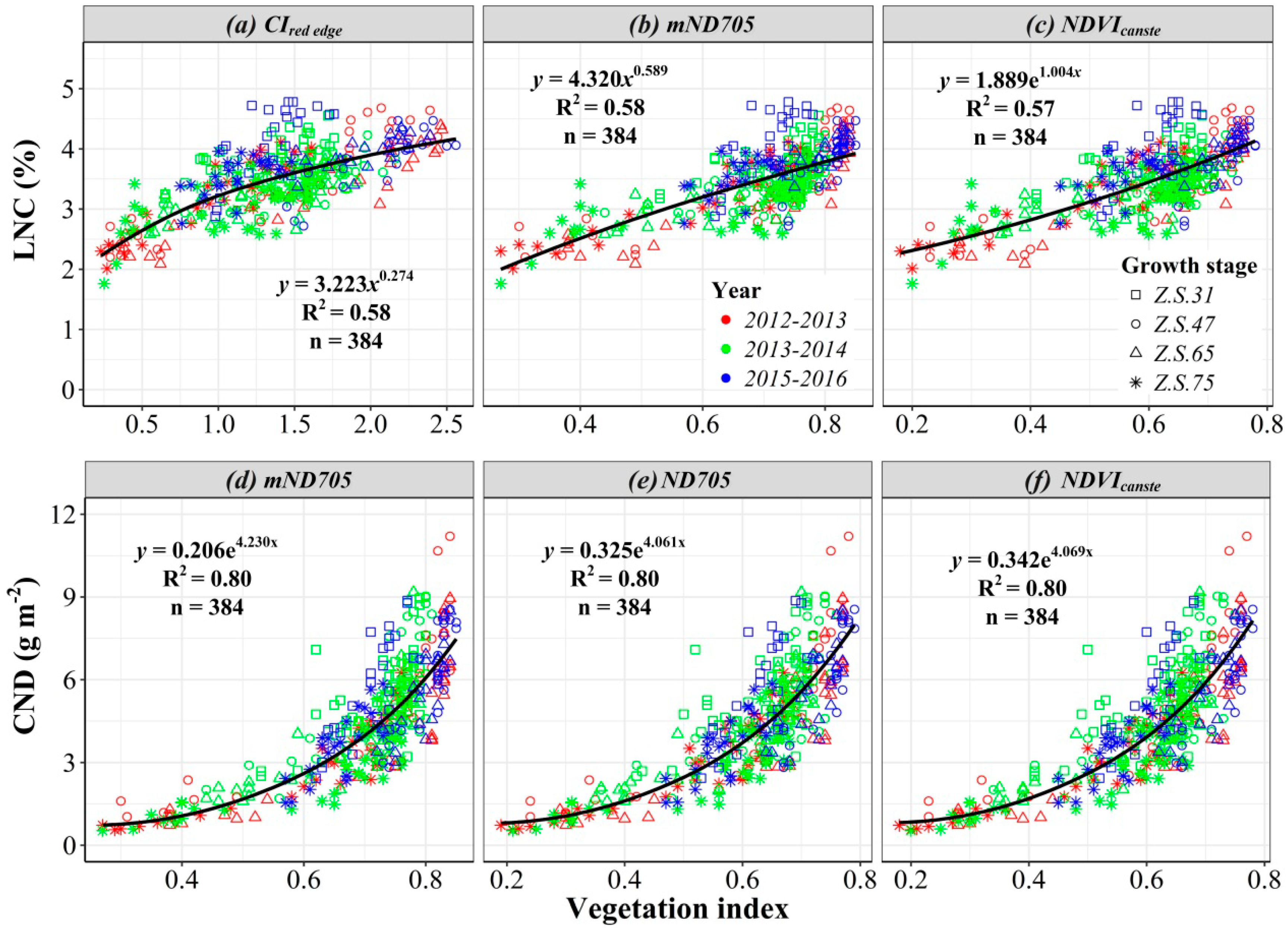
3.2. Correlations between Agronomic Variables and Vegetation Indices

Fifteen vegetation indices correlated with agronomic values were analyzed (Table 6). The results showed that all spectral indices were highly significantly related to LAI (p-value < 0.01) except NDLMA which had a correlation significant at the 0.05 level. The fourteen spectral indices except DCNI had correlations greater than 0.68, and MSR had the highest correlation with LAI, with r value of 0.80. Correlation coefficients between Cm and the spectral indices showed that fifteen vegetation indices, except DCNI, indicated highly significant differences (p-values < 0.01), but the absolute r values were only from 0.14 to 0.35, which were lower than the r values between LAI and the corresponding spectral indices. All spectral indices were highly significantly related to LND (p-value < 0.01). The maximum and minimum correlations were with MCARI/MTVI2 and NDLMA, with r values of −0.56 and −0.19, respectively. According to the correlations analysis, MSR, GI, and MCARI/MTVI2 were first used to develop the cost function in the N-PROSAIL model.
Correlations of LNC and CND to the fifteen vegetation indices were also analyzed (Table 6). The results showed that all vegetation indices, expect NDLMA, were identified as significantly correlated with LNC and CND, respectively. In particular, CIred edge, GNDVI, MCARI/MTVI2, mND705, ND705, SPVI, NDVIcanste, and NDRE showed relatively higher correlations with LNC (r ≥ 0.70) than the others, while CIred edge, GNDVI, MSR, ND705, WDRVI, SPVI, NDVIcanste, and NDRE exhibited higher correlations with CND (r ≥ 0.79) than the others. Therefore, these vegetation indices could be used to further establish regression models with the purpose of comparing and evaluating the performance of LNC and CND estimation using the N-PROSAIL model.

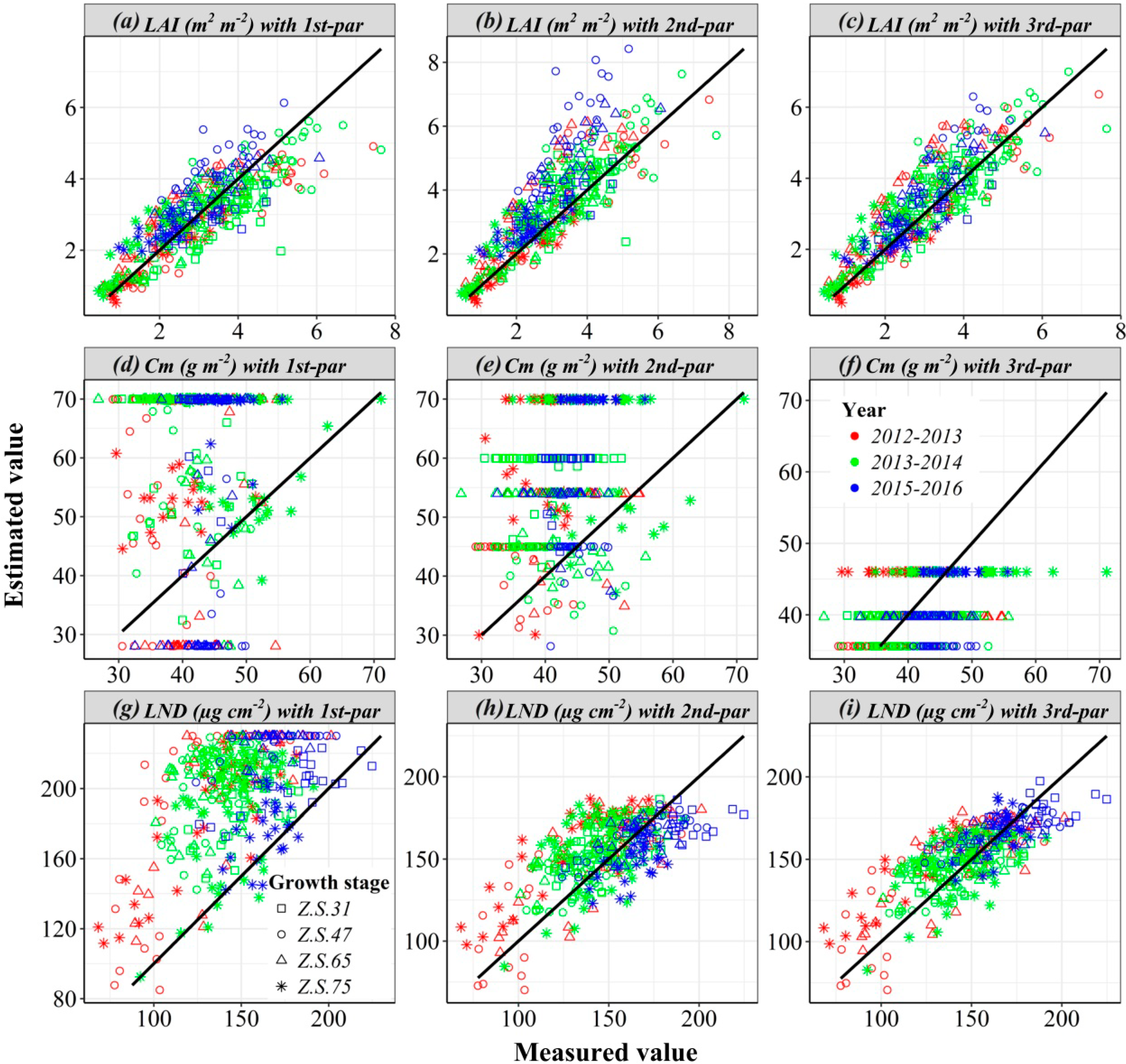
3.3. LAI, LND, and Cm Estimation Using the N-PROSAIL Model Inversion

The N-PROSAIL model using the SCE-UA method was first applied to retrieve LAI, Cm, and LND in this study. Three parameter settings, 1st-par setting, 2nd-par setting, and 3rd-par setting, were tried in this process in order to get the best estimation of LNC and CND. The retrieved results of each agronomic variable with each parameter setting are shown in Figure 3 and Table 7.
The results showed that a high consistency between the measured LAI and simulated LAI by the N-PROSAIL model inversion with the three parameter setting (Figure 3a–c). At different growth stages, the R2 and RMSE values between the simulated LAI and measured LAI for the 1st-par setting, the 2nd-par setting, and the 3rd-par setting ranged from 0.45–0.69 and 0.56–0.93, 0.45–0.68 and 0.61–1.46, and 0.59–0.70 and 0.55–0.88, respectively (Table 7). The 3rd-par setting exhibited a relatively higher R2 and lower RMSE than the other two parameter settings. The relationships between the simulated and measured LAIs at all growth stages were analyzed together, and the results showed that LAI estimation by the N-PROSAIL model inversion with the 3rd-par setting (R2 = 0.75 and RMSE = 0.73) was superior to the LAI estimation with the 1st-par setting (R2 = 0.67 and RMSE = 0.74) and the 2nd-par setting (R2 = 0.67 and RMSE = 1.08). The independent data of 2014–2015 was used to test the estimation performance, and LAI estimation with the 3rd-par setting (R2 = 0.80 and RMSE = 0.69) appeared stable compared with LAI estimation with the 1st-par setting (R2 = 0.81 and RMSE = 0.64) and the 2nd-par setting (R2 = 0.76 and RMSE = 0.93). These results indicated that the 3rd-par setting to retrieve LAI had the best estimation accuracy.
Cm estimations with the 1st-par setting and the 2nd-par setting in the N-PROSAIL model were achieved (Table 7 and Figure 3d–f). The results showed no significant difference between measured Cm and estimated Cm with the 2nd-par setting across the validation set and with the 3rd-par setting across the calibration and validation set. In the 1st-par setting, the interval of Cm at different growth period was not considered, and the limited range of Cm was set the same at all growth periods. Many estimation results were ranged on both sides of the interval, and there were relatively high deviations, with RMSE values of 23.79 and 27.93 g·m−2 for the calibration set and validation set, respectively (Figure 3d). The deviation between the measured Cm and estimated Cm was decreased to 16.12 and 18.50 g·m−2 for the calibration set and the validation set in the 2nd-par setting, where the interval of Cm values were based on the statistical results of the calibration set at different growth periods. However, many estimated values ranged on both sides of the interval as well (Figure 3e). Cm estimations with the 3rd-par setting in the N-PROSAIL model showed relatively lower RMSE than that of the 1st-par and 2nd-par setting, with RMSE values of 6.10 and 8.19 g m-2 for the calibration set and validation set, respectively. The results showed that Cm inversion using the optimizing algorithm of this study had a high deviation even given the limited ranges at different growth stages, and one Cm value at each growth stage had the lowest deviation in this study.
Finally, LND estimations with the three parameters setting in the N-PROSAIL model were compared (Table 7 and Figure 3g–i). The retrieval accuracy of LND was effectively improved after considering the optimizing parameters (the 2nd-par and 3rd-par settings), with R2 and RMSE values of 0.45 and 20.80 µg·cm−2 for the 2nd-par setting, and 0.59 and 17.43 µg·cm−2 for the 3rd-par setting, respectively. However, the R2 and RMSE values for the 1st-par setting were 0.30 and 58.49 µg·cm−2, respectively. The improvements at different growth stages were also significant compared with the 1st-par setting, with an increase in R2 by 0–0.13 and 0.14–0.28, and a decrease in RMSE by 21.78–51.47 µg·cm−2 and 27.08–52.78 µg·cm−2 for the 2nd-par setting and the 3rd-par setting, respectively. The phenomenon of overestimation at LND estimation by the N-PROSAIL model with the 1st-par setting was clear (Figure 3g). LND estimation with the optimized parameters setting (the 2nd-par setting and the 3rd-par setting) reduced the problem of LND overestimation. According to the above comparison, LND estimation with the 3rd-par setting had a slightly better performance than that with the 2nd-par setting (Figure 3h,i). The validation results showed that the best performance was produced by the 3rd-par setting (R2 = 0.46 and RMSE = 21.18 µg·cm−2), followed by the 2nd-par setting (R2 = 0.39 and RMSE = 24.15 µg·cm−2), and finally the 1st-par setting (R2 = 0.34 and RMSE = 62.86 µg·cm−2). Therefore, the LND estimation confirmed the operational potential of the N-PROSAIL model inversion with optimizing parameters, and the retrieval without considering Cm inversion had the best LND estimation.

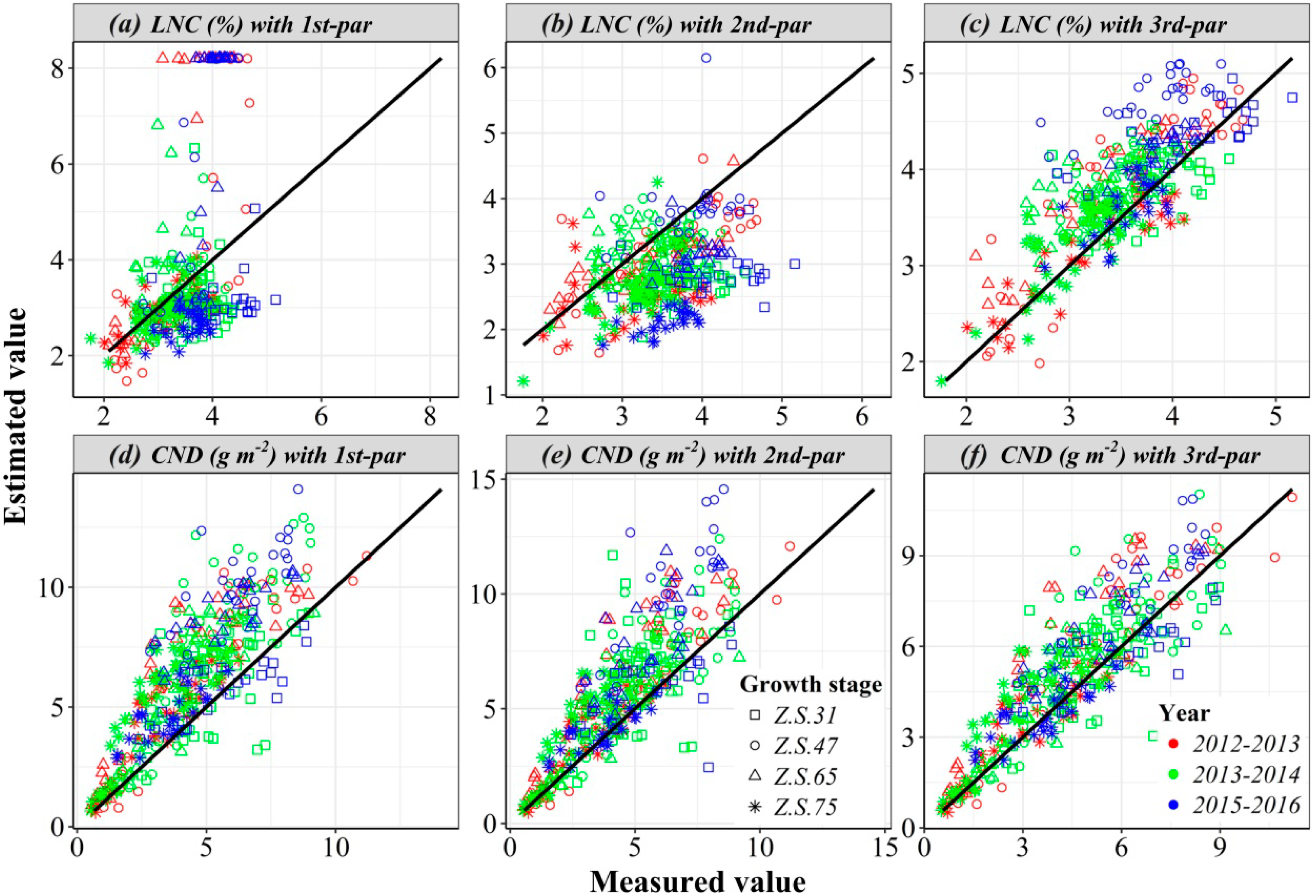
3.4. LNC and CND Estimation Based on LAI, LND, and Cm

The following estimations were to acquire LNC calculated by LND and Cm, and CND calculated by LAI and LND, respectively. The retrieved results of each agronomic variable with default parameters and optimized parameters were also compared in Figure 4 and Table 7.
Relative to the N-PROSAIL model inversion by the 1st-par and the 2nd-par setting, LNC estimation using the 3rd-par setting performed relatively better, with R2 and RMSE values of 0.62% and 0.48% for the calibration set. The inversion of the N-PROSAIL model by the 3rd-par setting at different growth stages was also estimated better than by the 1st-par and the 2nd-par setting (Table 7). Many LNC estimations were overestimated, which resulted from the overestimation of LND and Cm (Figure 3d,g and Figure 4a). The 2nd-par setting considering the parameter settings at different growth stages mitigated the overestimation of LNC, but LNC estimation did not performed well (R2 = 0.14 and RMSE = 0.87%). The independent data of 2014–2015 was used to validate the model stability, and the inversion of the N-PROSAIL model by the 3rd-par setting exhibited a superior result for LNC estimation with R2 and RMSE values of 0.75 and 0.38%. This study further showed that calibrating parameters at different growth stages is necessary, and the retrieval without considering Cm inversion achieved a satisfactory estimation for LNC.
Together, using the N-PROSAIL model, it was able to get CND on the basis of LAI and LND (Figure 4d–f). The R2 and RMSE values for the 1st-par setting at different growth stages ranged from 0.36 to 0.74 and 1.66 to 3.19 g·m−2, respectively, and their values at all growth stages were 0.66 and 2.45 g·m−2 (Table 7). CND estimations for the 2nd-par setting across different growth stages ranged from 0.20 to 0.73 and 1.24 to 2.57 g·m−2, respectively, and their values at all growth stages were 0.67 and 2.08 g·m−2 (Table 7). CND estimations for the 3rd-par setting showed a good performance, with a higher R2 values and lower RMSE values across different stages, and the R2 and RMSE values across different growth stages were 0.75 and 1.32 g·m−2, respectively. Then, the validation dataset was used to validate the model stability, and the model inversion with the 3rd-par setting (R2 = 0.82 and RMSE = 0.95 g·m−2) also performed better than the inversions with the 1st-par setting (R2 = 0.76 and RMSE = 1.47 g·m−2) and the 2nd-par setting (R2 = 0.82 and RMSE = 1.03 g·m−2). The results of this study suggest that the 3rd-par setting in the N-PROSAIL model inversion is the best choice.

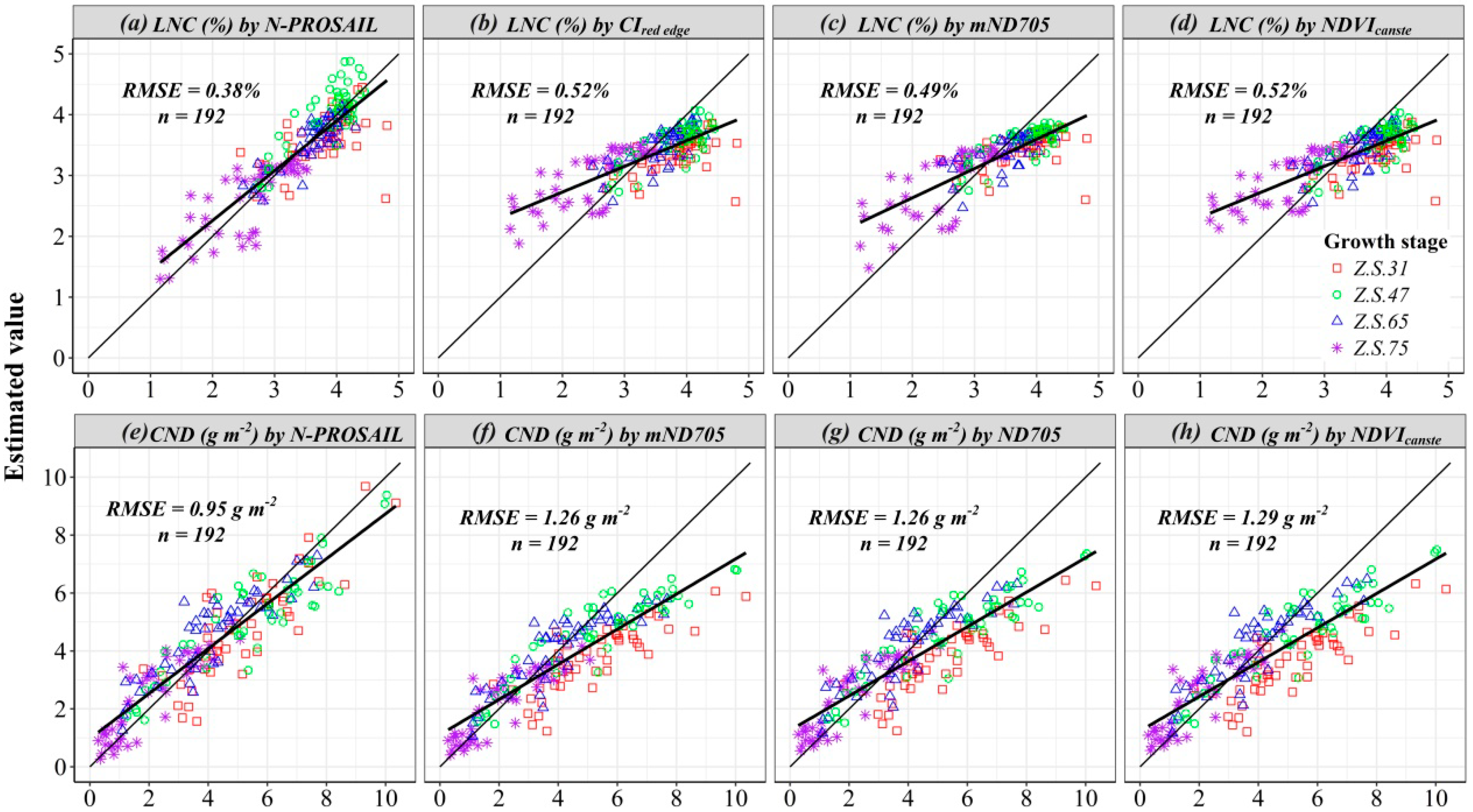
3.5. Comparison of the N-PROSAIL Model Method with the Vegetation Index Method

To evaluate the performance of LNC and CND estimation by the N-PROSAIL method with parameter optimization (estimations of LNC and CND with the 3rd-par setting were using in the following comparison), the estimation results using the N-PROSAIL model method were compared with the estimation results by the vegetation index method. Fourteen spectral indices with significant relationships were used to fit the regression models (Linear model, Power model, Exponential model, and logarithmic) of LNC, and the best regression model was selected as optimal regression models (Table 8). In these regression models, ten indices with R2 values for LNC and vegetation indices were greater than 0.50, seven were greater than 0.55, and CIred edge, mND705 and NDVIcanste had the highest R2 values of 0.58, 0.58, and 0.57, respectively (Figure 3a–c). Compared with LNC estimation using the N-PROSAIL model, the R2 value between the estimated LNC and measured LNC was 0.62, which was better than all the regression models by vegetation indices. The validation set was used to test the model accuracy, the estimated values and measured values were compared based on the RMSE (Table 8 and Figure 4a–d). The regression model between LNC and MCARI/MTVI2 had the lowest RMSE value of 0.48% among the fourteen regression models with the RMSE values ranging from 0.48% to 0.65% (Figure 5). The RMSE value from measured LNC and predicted LNC by the N-PROSAIL model was 0.38%, which was lower than the values from all regression models by vegetation index (Table 7 and Table 8). The results also showed that the consistency between the estimated values and the measured values of the N-PROSAIL method performed better than any vegetation index methods. The results showed that the N-PROSAIL model inversion could be a good method to estimate LNC.
Similar comparisons were obtained for CND estimation between the N-PROSAIL model and vegetation indices methods. A highly significant regression relationship between measured CND and estimated CND was demonstrated both for the N-PROSAIL model method and the vegetation indices methods. The R2 value between the estimated CND by the N-PROSAIL model and measured CND was 0.75. For the regression model by vegetation index, ten regression models with R2 values for CND estimation were greater than 0.75 (Table 8), and three regression models by mND705, ND705 and NDVIcanste were up to 0.80 (Figure 6d–f). The results of model validation from the validation set showed that the N-PROSAIL method (RMSE = 0.95 g·m−2) performed better than the vegetation indices methods (RMSE = 1.26 − 1.78 g·m−2) for estimation of CND (Table 8 and Figure 6). An advantage of stability using the N-PROSAIL model inversion was demonstrated. Furthermore, there are underestimations at high CND values using vegetation indices estimation, but the N-PROSAIL method could mitigate the phenomenon of underestimation. Overall, our results indicated that using the N-PROSAIL model with parameters optimizing has great potential for LNC and CND estimation in winter wheat.

4. Discussion

The N-PROSAIL model integrating the N-PROSPECT model and the SAILH model were developed to retrieve N status at leaf scale (LNC) and canopy scale (CND) [27,28]. LAI, Cm, and LND were retrieved from the N-PROSAIL model, and LNC and CND were calculated according to these relationships. LND had more variability on LNC than Cm. LNC showed a strong correlation with LND (r = 0.73) and relative low correlation with Cm (r = −0.19). This is because Cm is mainly determined by the plant cultivars and growth stage, and has little change when certain other conditions change [35]. But LND composed of two compartments, high N concentration in metabolic tissues and low N concentration in plant architecture, changes dynamically with plant growth [56]. Therefore, the results indicated the effect of LND on LNC estimation to be more sensitive to the effect from Cm. At the canopy scale, CND strongly reflects the variability of LAI (r = 0.90) as LND was relatively stable (r = 0.52). At different growth stages, canopy information, e.g., LAI, varied significantly, especially the variation between two growth stages [22,30]. This is explained by the lower coefficient of variation of LND compared to LAI (Table 5). This conclusion is in agreement with the study of Darvishzadeh [30], who found that canopy chlorophyll content was more related to LAI with an r value of 0.94.
According to the results of LAI, Cm, and LND estimations, the relationship between measured LAI and its estimation reflects more consistence and accuracy than LND and Cm (Figure 3). The main reasons are as follows: (1) LAI is the canopy characteristics and one of the variables most affected by canopy reflectance, while Cm and LND are variables at leaf level and their variations were lower than LAI; (2) the most correlated vegetation indices between these three variables were selected to build the cost function. LAI showed best correlation with MSR (r = 0.80) and was also highly correlated with MCARI/MTVI2 (r = −0.69) and GI (r = 0.79) (Table 6). The deviation was also relatively lower than with the other two variables. The study result is in line with the findings of previous studies by Feret et al. [57], Darvishzadeh et al. [30], and Li et al. [26].
In this study, three inversion strategies of estimating LNC and CND were tried in order to improve the estimation accuracy. In the 1st-par setting, LAI, Cm, and LND were considered for retrieval, and the other parameters in the N-PROSAIL model were set default values. The results showed that many Cm values were estimated at both sides of the interval and overestimations of LND were obvious. The estimations of these three variables were improved by prior parameters initialization, which is to limit the interval of the three values and assigning different values to the other parameters at different growth stages (the 2nd-par setting). The RMSE of Cm between estimated and measured values greatly decreased from 27.93 to 18.50 g·m−2, and the overestimation of LND was eliminated (Figure 3 and Table 7). These resulted in the improvement of LNC and CND estimation, with higher R2 values of 0.51 and 0.82 and lower RMSE values of 0.94% and 1.03 g·m−2 for LNC and CND, respectively. The results indicated the necessity of giving different values of non-optimizing parameters in the N-PROSAIL model at different growth stages. As shown in this study, the statistical values of Cw and calibrating solar zenith angle varied as plant growth progressed, and N and LID also showed difference at different growth stages (Table 3). The uncertainties of model inversion were reduced through giving the different values to these parameters at different growth stages. In the 3rd-par setting, we attempted not to retrieve the Cm value and set the mean values of Cm at each growth stage as the model input. The 3rd-par setting showed more improvement than the 2nd-par setting. The lower RMSE, 8.19 g·m−2, for Cm between estimated and measured values demonstrated the lower certainty than the above two parameters setting, and the inversion of LAI and LND were also improved (Table 7). It has two explanations for this: (1) one parameter decreased can reduce the ill-posed problem in model parameters inversion (Figure 3d–f) [29,30]; (2) Cm is an important parameter in the crop growth model and has one initial value for specific crop cultivars and changes as growth goes on [35,36]. Jacquemoud indicated that Cm was first assumed a constant for one plant in the PROSPECT model construction [37]. Thus, the 3rd-par setting considered as a default value at each growth stage is reasonable. The estimated performance for every variable with the 3rd-par setting also exhibits the highest accuracy. Therefore, using the 3rd-par setting in the N-PROSAIL model is a better strategy for estimating plant N status.
CIred edge, mND705 and NDVIcanste were selected as the best three vegetation indices to estimate LNC. They all showed overestimation at low LNC and these samples were mainly measured at Z.S. 75. CND estimation by mND705, ND705, and NDVIcanste demonstrated the same phenomenon, with CND estimation at a high value and at Z.S. 31 showed underestimation. Estimated LNC and CND using the N-PROSAIL model showed a higher accuracy than using vegetation indices. Two advantages of using the N-PROSAIL model can explain the situation. Firstly, estimating LAI and LND by the N-PROSAIL model are interactional. The two parameters are retrieved all at once and adjusted according to changes to each other, and are acquired relatively accurately in the end. So LNC and CND estimations were taken into account the results of LAI and LND. Secondly, different parameters, except LAI and LND in N-PROSAIL, were calibrated as different values at various growth stages, which greatly reduced the deviation of model. The improvement of this step was significant according to the compared results of 1st-par setting and 3rd-par setting (Figure 4).
The results showed the potential of a priori information (setting different parameters values at various growth stages) in using N-PROSAIL model for LNC and CND retrieval in winter wheat, which is also suitable to apply in other crops (rice, maize, cotton, etc.) by giving corresponding crop parameters values. However, it is still necessary to define this information as accurately as possible. Four critical growth stages in winter wheat were selected in this study and parameters in the N-PROSAIL model at different growth stages were set respectively. Further studies should focus on considering more growth stages or a high temporal resolution [58], and in this situation, the considered fixed parameters set across different growth stage will increase. The estimation accuracy will be influenced if the growth stage was determined inaccurately. Moreover, fixed parameters were determined in the study area. Further studies should verify whether these parameters change across different regions. Future research should also focus on validating the model using multi-platforms, such as unmanned aerial vehicle and satellite platform. The study should finally point that accurate plant N estimation is an important step towards precision N management, and more studies are needed to develop N-PROSAIL model-based in-season N recommendation algorithms and management strategies.

5. Conclusions

In this study, the N-PROSAIL model was established to retrieve winter wheat LNC and CND at different growth stages. The results suggested that:
(1) The 3rd-par setting retrieval strategies with LAI and LND optimized and other parameters in the N-PROSAIL model fixed at each growth stage exhibited the highest accuracy. The retrieved LAI (R2 = 0.80 and RMSE = 0.69) and LND (R2 = 0.46 and RMSE = 21.18 µg·cm−2) were consistent with the measured LAI and LND, respectively.
(2) LNC and CND were accurately estimated using the N-PROSAIL model, with R2 and RMSE values of 0.75 and 0.38%, and 0.82 and 0.95 g·m−2, respectively.
(3) Compared with vegetation indices regression model, the N-PROSAIL model results reduced the problems of overestimation at low LNC and underestimation at high CND, and showed better performance than any vegetation index regression model (LNC: RMSE = 0.48−0.64%; CND: 1.26−1.78 g·m−2). The N-PROSAIL model shows a great potential to estimate canopy N status at leaf and canopy scales in winter wheat.

Author Contributions

G.Y., Z.L. (Zhenhai Li) and C.Z. conceived and designed the experiments; Z.L. (Zhenhai Li) and H.Y. performed the experiments; Z.L. (Zhenhai Li) and X.J. analyzed the data; Z.L. (Zhenhai Li), Z.L. (Zhenhong Li) and C.Z. discussed and drafted the manuscript. Z.L. (Zhenhong Li), J.D. and B.C. revised the manuscript and edited English language. All authors read and approved the final version.

Funding

This study was supported by the National Natural Science Foundation of China (Grant No. 61661136003, 41471285, 41601369), the UK Science and Technology Facilities Council through the PAFiC project (Ref: ST/N006801/1), the Open Research Fund of Key Laboratory of Digital Earth Science, Institute of Remote Sensing and Digital Earth, Chinese Academy of Sciences (No. 2016LDE008), and the National Key Technologies of Research and Development Program (2016YFD0300602-04).

Acknowledgments

We are grateful to Weiguo Li, Hong Chang and Ling Kong for data collection.

Conflicts of Interest

The authors declare no conflict of interest.

References

  1. Yao, X.; Huang, Y.; Shang, G.; Zhou, C.; Cheng, T.; Tian, Y.; Cao, W.; Zhu, Y. Evaluation of Six Algorithms to Monitor Wheat Leaf Nitrogen Concentration. Remote Sens. 2015, 7, 14939–14966. [Google Scholar] [CrossRef] [Green Version]
  2. Li, F.; Miao, Y.; Hennig, S.D.; Gnyp, M.L.; Chen, X.; Jia, L.; Bareth, G. Evaluating hyperspectral vegetation indices for estimating nitrogen concentration of winter wheat at different growth stages. Precis. Agric. 2010, 11, 335–357. [Google Scholar] [CrossRef]
  3. Karimi, Y.; Prasher, S.O.; Patel, R.M.; Kim, S.H. Application of support vector machine technology for weed and nitrogen stress detection in corn. Comput. Electron. Agric. 2006, 51, 99–109. [Google Scholar] [CrossRef]
  4. Miphokasap, P.; Honda, K.; Vaiphasa, C.; Souris, M.; Nagai, M. Estimating Canopy Nitrogen Concentration in Sugarcane Using Field Imaging Spectroscopy. Remote Sens. 2012, 4, 1651–1670. [Google Scholar] [Green Version]
  5. Kokaly, R.F. Investigating a Physical Basis for Spectroscopic Estimates of Leaf Nitrogen Concentration. Remote Sens. Environ. 2001, 75, 153–161. [Google Scholar] [CrossRef]
  6. Niu, Z.; Chen, Y.; Sui, Z.; Zhang, Q.Y.; Zhao, C.J. Mechanism Analysis of Leaf Biochemical Concentration by High Spectral Remote Sensing. J. Remote Sens. 2000, 4, 125–130. [Google Scholar]
  7. Cho, M.A.; Skidmore, A.K. A new technique for extracting the red edge position from hyperspectral data: The linear extrapolation method. Remote Sens. Environ. 2006, 101, 181–193. [Google Scholar] [CrossRef]
  8. Barnes, E.M.; Clarke, T.R.; Richards, S.E.; Colaizzi, P.D.; Haberland, J.; Kostrzewski, M.; Waller, P.; Choi, C.; Riley, E.; Thompson, T.; et al. Coincident Detection of crop Water Stress, Nitrogen Status and Canopy Density Using Ground-Based Multispectral Data. Available online: https://naldc.nal.usda.gov/download/4190/PDF (accessed on 11 September 2018).
  9. Serrano, L.; Peñuelas, J.; Ustin, S.L. Remote sensing of nitrogen and lignin in Mediterranean vegetation from AVIRIS data: Decomposing biochemical from structural signals. Remote Sens. Environ. 2002, 81, 355–364. [Google Scholar] [CrossRef]
  10. Fitzgerald, G.J.; Rodriguez, D.; Christensen, L.K.; Belford, R.; Sadras, V.O.; Clarke, T.R. Spectral and thermal sensing for nitrogen and water status in rainfed and irrigated wheat environments. Precis. Agric. 2006, 7, 233–248. [Google Scholar]
  11. Feng, W.; Yao, X.; Zhu, Y.; Tian, Y.C.; Cao, W.X. Monitoring leaf nitrogen status with hyperspectral reflectance in wheat. Eur. J. Agron. 2008, 28, 394–404. [Google Scholar] [CrossRef]
  12. Fitzgerald, G.; Rodriguez, D.; O’Leary, G. Measuring and predicting canopy nitrogen nutrition in wheat using a spectral index—The canopy chlorophyll content index (CCCI). Field Crop. Res. 2010, 116, 318–324. [Google Scholar] [CrossRef]
  13. Chen, P.; Haboudane, D.; Tremblay, N.; Wang, J.; Vigneault, P.; Li, B. New spectral indicator assessing the efficiency of crop nitrogen treatment in corn and wheat. Remote Sens. Environ. 2010, 114, 1987–1997. [Google Scholar] [CrossRef] [Green Version]
  14. Tian, Y.C.; Yao, X.; Yang, J.; Cao, W.X.; Hannaway, D.B.; Zhu, Y. Assessing newly developed and published vegetation indices for estimating rice leaf nitrogen concentration with ground-and space-based hyperspectral reflectance. Fuel Energy Abstr. 2011, 120, 299–310. [Google Scholar] [CrossRef]
  15. Yao, X.; Jia, W.; Si, H.; Guo, Z.; Tian, Y.; Liu, X.; Cao, W.; Zhu, Y. Exploring novel bands and key index for evaluating leaf equivalent water thickness in wheat using hyperspectra influenced by nitrogen. PLoS ONE 2014, 9, e96352. [Google Scholar] [CrossRef] [PubMed]
  16. Feng, W.; Zhang, H.Y.; Zhang, Y.S.; Qi, S.L.; Heng, Y.R.; Guo, B.B.; Ma, D.Y.; Guo, T.C. Remote detection of canopy leaf nitrogen concentration in winter wheat by using water resistance vegetation indices from in-situ hyperspectral data. Field Crop. Res. 2016, 198, 238–246. [Google Scholar] [CrossRef]
  17. Elshikha, D.M.; Barnes, E.M.; Clarke, T.R.; Hunsaker, D.J.; Haberland, J.A.; Pinter, P.J.; Waller, P.M.; Thompson, T.L. Remote Sensing of Cotton Nitrogen Status Using the Canopy Chlorophyll Content Index (CCCI). Trans. Asabe 2008, 51, 73–82. [Google Scholar]
  18. Hansen, P.M.; Schjoerring, J.K. Reflectance measurement of canopy biomass and nitrogen status in wheat crops using normalized difference vegetation indices and partial least squares regression. Remote Sens. Environ. 2003, 86, 542–553. [Google Scholar] [CrossRef]
  19. Ecarnot, M.; Compan, F.; Roumet, P. Assessing leaf nitrogen content and leaf mass per unit area of wheat in the field throughout plant cycle with a portable spectrometer. Field Crop. Res. 2013, 140, 44–50. [Google Scholar] [CrossRef]
  20. Li, L.; Lu, J.; Wang, S.; Ma, Y.; Wei, Q.; Li, X.; Cong, R.; Ren, T. Methods for estimating leaf nitrogen concentration of winter oilseed rape (Brassica napus L.) using in situ, leaf spectroscopy. Ind. Crop. Prod. 2016, 91, 194–204. [Google Scholar] [CrossRef]
  21. Zhang, C.; Kovacs, J.M.; Wachowiak, M.P.; Flores-Verdugo, F. Relationship between Hyperspectral Measurements and Mangrove Leaf Nitrogen Concentrations. Remote Sens. 2013, 5, 891–908. [Google Scholar] [CrossRef] [Green Version]
  22. Xu, X.G.; Zhao, C.J.; Wang, J.H.; Li, C.J.; Yang, X.D. Associating new spectral features from visible and near infrared regions with optimal combination principle to monitor leaf nitrogen concentration in barley. J. Infrared Millim. Waves 2013, 32, 351. [Google Scholar] [CrossRef]
  23. Xu, X.G.; Zhao, C.J.; Wang, J.H.; Zhang, J.C.; Song, X.Y. Using optimal combination method and in situ hyperspectral measurements to estimate leaf nitrogen concentration in barley. Precis. Agric. 2014, 15, 227–240. [Google Scholar] [CrossRef]
  24. Li, Z.; Nie, C.; Wei, C.; Xu, X.; Song, X.; Wang, J. Comparison of Four Chemometric Techniques for Estimating Leaf Nitrogen Concentrations in Winter Wheat (Triticum aestivum) Based on Hyperspectral Features. J. Appl. Spectrosc. 2016, 83, 240–247. [Google Scholar] [CrossRef]
  25. Atzberger, C. Object-based retrieval of biophysical canopy variables using artificial neural nets and radiative transfer models. Remote Sens. Environ. 2004, 93, 53–67. [Google Scholar] [CrossRef]
  26. Li, Z.; Jin, X.; Wang, J.; Yang, G.; Nie, C.; Xu, X.; Feng, H. Estimating winter wheat (Triticum aestivum) LAI and leaf chlorophyll content from canopy reflectance data by integrating agronomic prior knowledge with the PROSAIL model. Int. J. Remote Sens. 2015, 36, 2634–2653. [Google Scholar] [CrossRef]
  27. Yang, G.; Zhao, C.; Pu, R.; Feng, H.; Li, Z.; Li, H.; Sun, C. Leaf nitrogen spectral reflectance model of winter wheat (Triticum aestivum) based on PROSPECT: simulation and inversion. J. Appl. Remote Sens. 2015, 9. [Google Scholar] [CrossRef]
  28. Verhoef, W. Light scattering by leaf layers with application to canopy reflectance modeling: the SAIL model. Remote Sens. Environ. 1984, 16, 125–141. [Google Scholar] [CrossRef]
  29. Combal, B.; Baret, F.; Weiss, M.; Trubuil, A.; Mace, D.; Pragnere, A.; Myneni, R.; Knyazikhin, Y.; Wang, L. Retrieval of canopy biophysical variables from bidirectional reflectance: Using prior information to solve the ill-posed inverse problem. Remote Sens. Environ. 2002, 84, 1–15. [Google Scholar] [CrossRef]
  30. Darvishzadeh, R.; Skidmore, A.; Schlerf, M.; Atzberger, C. Inversion of a radiative transfer model for estimating vegetation LAI and chlorophyll in a heterogeneous grassland. Remote Sens. Environ. 2008, 112, 2592–2604. [Google Scholar] [CrossRef]
  31. Zadoks, J.C.; Chang, T.T.; Konzak, C.F. A decimal code for the growth stages of cereals. Weed Res. 1974, 14, 415–421. [Google Scholar] [CrossRef]
  32. Liu, L.; Song, B.; Zhang, S.; Liu, X. A Novel Principal Component Analysis Method for the Reconstruction of Leaf Reflectance Spectra and Retrieval of Leaf Biochemical Contents. Remote Sens. 2017, 9. [Google Scholar] [CrossRef]
  33. Schepers, J.S.; Francis, D.D.; Thompson, M.T. Simultaneous determination of total C, total N, and 15N on soil and plant material 1. Commun. Soil Sci. Plant Anal. 1989, 20, 949–959. [Google Scholar] [CrossRef]
  34. Wang, J.; Zhao, C.; Huang, W. Quantitative Remote Sensing of Agriculture: Theory and Application; Science Press: Beijing, China, 2008. (In Chinese) [Google Scholar]
  35. Jones, J.W.; Hoogenboom, G.; Porter, C.H.; Boote, K.J.; Batchelor, W.D.; Hunt, L.A.; Wilkens, P.W.; Singh, U.; Gijsman, A.J.; Ritchie, J.T. The DSSAT cropping system model. Eur. J. Agron. 2003, 18, 235–265. [Google Scholar] [CrossRef]
  36. Boogaard, H.L.; Diepen, C.A.; Rotter, R.P.; Cabrera, J.A.; Laar, H.H. User’s guide for the WOFOST 7.1 Crop Growth Simulation Model and WOFOST Control Center. Available online: http://library.wur.nl/WebQuery/wurpubs/309027 (accessed on 11 September 2018).
  37. Jacquemoud, S.; Baret, F. PROSPECT: A model of leaf optical properties spectra. Remote Sens. Environ. 1990, 34, 75–91. [Google Scholar] [CrossRef]
  38. Gitelson, A.A.; Vina, A.; Ciganda, V.; Rundquist, D.C.; Arkebauer, T.J. Remote estimation of canopy chlorophyll content in crops. Geophys. Res. Lett. 2005, 32. [Google Scholar] [CrossRef]
  39. Baret, F.; Guyot, G. Potentials and limits of vegetation indices for LAI and APAR assessment. Remote Sens. Environ. 1991, 35, 161–173. [Google Scholar] [CrossRef]
  40. Eitel, J.U.H.; Long, D.S.; Gessler, P.E.; Smith, A.M.S. Using in-situ measurements to evaluate the new RapidEye™ satellite series for prediction of wheat nitrogen status. Int. J. Remote Sens. 2007, 28, 4183–4190. [Google Scholar] [CrossRef]
  41. Sims, D.A.; Gamon, J.A. Relationships between leaf pigment content and spectral reflectance across a wide range of species, leaf structures and developmental stages. Remote Sens. Environ. 2002, 81, 337–354. [Google Scholar] [CrossRef]
  42. Chen, J.M. Evaluation of vegetation indices and a modified simple ratio for boreal applications. Can. J. Remote Sens. 1996, 22, 229–242. [Google Scholar] [CrossRef]
  43. Pearson, R.L.; Miller, L.D. Remote Mapping of Standing Crop Biomass for Estimation of the Productivity of the Shortgrass Prairie. Available online: http://adsabs.harvard.edu/abs/1972rse.conf.1355P (accessed on 11 September 2018).
  44. Le Maire, G.; François, C.; Soudani, K.; Berveiller, D.; Pontailler, J.Y.; Bréda, N.; Genet, H.; Davi, H.; Dufrêne, E. Calibration and validation of hyperspectral indices for the estimation of broadleaved forest leaf chlorophyll content, leaf mass per area, leaf area index and leaf canopy biomass. Remote Sens. Environ. 2008, 112, 3846–3864. [Google Scholar] [CrossRef]
  45. Gitelson, A.A. Wide dynamic range vegetation index for remote quantification of biophysical characteristics of vegetation. J. Plant Physiol. 2004, 161, 165–173. [Google Scholar] [CrossRef] [PubMed]
  46. Delalieux, S.; Somers, B.; Hereijgers, S.; Verstraeten, W.W.; Keulemans, W.; Coppin, P.A. near-infrared narrow-waveband ratio to determine Leaf Area Index in orchards. Remote Sens. Environ. 2008, 112, 3762–3772. [Google Scholar] [CrossRef]
  47. Zarco-Tejada, P.J.; Berjón, A.; López-Lozano, R.; Miller, J.R.; Martín, P.; Cachorro, V.; González, M.R.; De Frutos, A. Assessing vineyard condition with hyperspectral indices: Leaf and canopy reflectance simulation in a row-structured discontinuous canopy. Remote Sens. Environ. 2005, 99, 271–287. [Google Scholar] [CrossRef]
  48. Vincini, M.; Frazzi, E.; D’Alessio, P. Angular Dependence of Maize and Sugar Beet VIs from Directional CHRIS/Proba Data. Available online: https://www.researchgate.net/publication/228413259_Angular_dependence_of_maize_and_sugar_beet_VIs_from_directional_CHRISProba_data (accessed on 11 September 2018).
  49. Steddom, K.; Heidel, G.; Jones, D.; Rush, C.M. Remote detection of rhizomania in sugar beets. Phytopathology 2003, 93, 720–726. [Google Scholar] [CrossRef] [PubMed]
  50. Duan, Q.Y.; Gupta, V.K.; Sorooshian, S. Shuffled complex evolution approach for effective and efficient global minimization. J. Optim. Theory Appl. 1993, 76, 501–521. [Google Scholar] [CrossRef]
  51. Duan, Q.; Sorooshian, S.; Gupta, V.K. Optimal use of the SCE-UA global optimization method for calibrating watershed models. J. Hydrol. 1994, 158, 265–284. [Google Scholar] [CrossRef] [Green Version]
  52. Zhu, X.; Zhao, Y.; Feng, X. A methodology for estimating Leaf Area Index by assimilating remote sensing data into crop model based on temporal and spatial knowledge. Chin. Geogr. Sci. 2013, 23, 550–561. [Google Scholar] [CrossRef] [Green Version]
  53. Jin, H.; Wang, J.; Bo, Y.; Chen, G.; Xue, H. Data Assimilation of MODIS and TM Observations into CERES-Maize Model to Estimate Regional Maize Yield. Available online: https://0-doi-org.brum.beds.ac.uk/10.1117/12.860315 (accessed on 11 September 2018).
  54. Wang, H.; Zhu, Y.; Li, W.; Cao, W.; Tian, Y. Integrating remotely sensed leaf area index and leaf nitrogen accumulation with RiceGrow model based on particle swarm optimization algorithm for rice grain yield assessment. J. Appl. Remote Sens. 2014, 8. [Google Scholar] [CrossRef]
  55. Huang, J.; Ma, H.; Su, W.; Zhang, X.; Huang, Y.; Fan, J.; Wu, W. Jointly assimilating MODIS LAI and ET products into the SWAP model for winter wheat yield estimation. IEEE J. Sel. Top. Appl. Earth Obs. Remote Sens. 2015, 8, 4060–4071. [Google Scholar] [CrossRef]
  56. Lemaire, G.; Jeuffroy, M.H.; Gastal, F. Diagnosis tool for plant and crop N status in vegetative stage: Theory and practices for crop N management. Eur. J. Agron. 2008, 28, 614–624. [Google Scholar] [CrossRef]
  57. Feret, J.B.; François, C.; Asner, G.P.; Gitelson, A.A.; Martin, R.E.; Bidel, L.P.; Ustin, S.L.; Le Maire, G.; Jacquemoud, S. PROSPECT-4 and 5: Advances in the leaf optical properties model separating photosynthetic pigments. Remote Sens. Environ. 2008, 112, 3030–3043. [Google Scholar] [CrossRef]
  58. Koetz, B.; Baret, F.; Poilvé, H.; Hill, J. Use of coupled canopy structure dynamic and radiative transfer models to estimate biophysical canopy characteristics. Remote Sens. Environ. 2005, 95, 115–124. [Google Scholar] [CrossRef]
Figure 1. Study site and experiment plot.
Remotesensing 10 01463 g001
Figure 2. Flowchart of estimating leaf N concentration (LNC) and canopy N density (CND) with the N-PROSAIL model and the Shuffled Complex Evolution method developed at the University of Arizona (SCE-UA) method.
Remotesensing 10 01463 g002
Figure 3. Comparison of measured and estimated values of leaf area index (LAI) (ac), Cm (df), and LND (gi) based on the N-PROSAIL model in winter wheat across the calibration set.
Remotesensing 10 01463 g003
Figure 4. Comparison of measured and estimated values of LNC (ac) and CND (df) based on the N-PROSAIL model in winter wheat across the calibration set.
Remotesensing 10 01463 g004
Figure 5. The relationships between measured and estimated values of LNC (ad) and CND (eh) in winter wheat by using data from 2014–2015 (n = 192).
Remotesensing 10 01463 g005
Figure 6. The best three regression models by vegetation index for LNC (ac) and CND (df) estimation in winter wheat across the calibration set (n = 384).
Remotesensing 10 01463 g006
Table 1. Summary of cultivar, soil characteristics and treatments for the four experiments.
No.SeasonCultivarTreatmentsDataset
Exp. 12012–2013Nongda211, Zhongmai175, Jing9843, Zhongyou206N rate (kg N ha−1):
0, 110, 220, 440
Calibration
Exp. 22013–2014Jing9843, Zhongmai175N rate (kg N ha−1):
0, 90, 180, 270;
Irrigation rate (mm):
0, 146, 292
Calibration
Exp. 32014–2015Jing9843, Zhongmai175N rate (kg N ha−1):
0, 90, 180, 270;
Irrigation rate (mm):
0, 192, 384
Validation
Exp. 42015–2016Lunxuan167, Jingdong18N rate (kg N ha−1):
18, 90, 180, 270;
Calibration
Table 2. List of acquired experiment data in the four wheat experiments.
Growth StageZadoksDateNo.LAICmLNDLNCCNDSpectral
Exp. 1: 2012–2013
Stem elongation3123 Apr.32--
Booting476 May32
Anthesis6519 May32
Milk development751 Jun.32
Exp. 2: 2013–2014
Stem elongation3311 Apr.48
Booting4520 Apr.48
Anthesis657 May48
Milk development7520 May48
Exp. 3: 2014–2015
Stem elongation3114 Apr.48
Booting4726 Apr.48
Anthesis6512 May48
Milk development7526 May48
Exp. 4: 2015–2016
Stem elongation3115 Apr.24
Booting4729 Apr.24
Anthesis6511 May24
Milk development7526 May24
Table 3. Specific ranges and setting for input parameters in the N-PROSAIL model.
Parameters1st-par Setting2nd-par/3rd-par Setting
Z.S. 3.1Z.S. 47Z.S. 65Z.S. 75
Leaf N density (LND, µg·cm−2)60–23075–23070–20080–20060–200
Leaf area index (LAI, m2·m−2)0.4–8.51.5–6.51.0–8.50.5–7.00.3–4.5
Dry matter content (Cm, g·m−2)4023–60 #; 40 ##28–45 #; 36 ##30–54 #; 39 ##30–70 #; 46 ##
Equivalent water content (Cw, cm)0.0100.01380.01270.00980.0085
Leaf structure parameter (Ns)1.51.241.071.031.16
Leaf inclination distribution (LID, deg)5050.547.245.043.8
Soil brightness parameter (Rsoil)0.440.490.730.620.35
Hot spot parameter (SL)0.150.240.100.120.21
Solar zenith angle (θs, deg)4530252218
# The ranges of Cm at the 2nd-par setting according to calibration dataset; ## the ranges of Cm at the 3rd-par setting according to calibration dataset.
Table 4. Summary of vegetation indices studied for the N-PROSAIL inversion and N estimation.
Vegetation IndexFormulationReference
CIred edge(R750/R720) − 1Gitelson et al. [38]
GNDVI(R750R550)/(R750 + R550)Baret et al. [39]
MCARI/MTVI2MCARI/MTVI2;
MCARI: (R700R670 − 0.2(R700R550))(R700/R670);
MTVI2: 0.5(1.2(R800R500)-2.5(R670R550))/
sqrt (2(R800 + 1)2 − (6R800 − 5sqrt(R670)) − 0.5)
Eitel et al. [40]
mND705(R750 - R705)/(R750 + R705 − 2R445)Sims et al. [41]
MSR(R800/R670 − 1)/sqrt(R800/R670 + 1)Chen [42]
ND705(R750R705)/(R750 + R705)Sims et al. [41]
NDVI(R890R670)/(R890 + R670)Pearson et al. [43]
NDLMA(R2260R1490)/(R2260 + R1490)Le Maire et al. [44]
DCNI(R720R700)/(R700R670)/(R720R670 + 0.03)Chen et al. [13]
WDRVI(0.1R890R670)/(0.1R890 + R670)Gitelson et al. [45]
sLAIDIs(R1050R1250)/(R1050 + R1250), s = 5Delalieux et al. [46]
GIR551/R677Zarco-Tejada et al. [47]
SPVI0.4(3.7(R800R670) − 1.2abs(R550R670))Vincini et al. [48]
NDVIcanste(R760R708)/(R760 + R708)Steddom et al. [49]
NDRE(R790R720)/(R790 + R720)Fitzgerald et al. [12]
Table 5. Correlations between agronomic variables (n = 384).
VariableLAICmLNDLNC
Cm−0.55 **
LND0.22 **0.45 **
LNC0.66 **-0.19 **0.73 **
CND0.90 **-0.30 **0.52 **0.84 **
** Model significance at the 0.01 probability level (p < 0.01).
Table 6. Correlations between agronomic variables and vegetation indices (n = 384).
VariableLAICmLNDLNCCND
CIred edge0.76 **−0.22 **0.49 **0.70 **0.81 **
GNDVI0.77 **−0.21 **0.49 **0.70 **0.79 **
MCARI/MTVI2−0.69 **0.14 **−0.56 **−0.71 **−0.75 **
mND7050.74 **−0.21 **0.52 **0.73 **0.78 **
MSR0.80 **−0.28 **0.41 **0.67 **0.81 **
ND7050.76 **−0.23 **0.50 **0.71 **0.79 **
NDVI0.74 **−0.23 **0.47 **0.68 **0.75 **
NDLMA0.12*−0.26 **−0.19 **0.00 #0.06 #
DCNI0.40 **−0.01 #0.45 **0.48 **0.49 **
WDRVI0.79 **−0.27 **0.44 **0.68 **0.80 **
sLAIDI0.68 **−0.20 **0.38 **0.56 **0.69 **
GI0.79 **−0.35 **0.30 **0.61 **0.76 **
SPVI0.79 **−0.28 **0.44 **0.71 **0.82 **
NDVIcanste0.76 **−0.22 **0.51 **0.72 **0.79 **
NDRE0.74 **−0.19 **0.52 **0.71 **0.79 **
* Model significance at the 0.05 probability level (p < 0.05); ** Model significance at the 0.01 probability level (p < 0.01); # Model with no significance.
Table 7. Comparison of different agronomic parameters estimation with different parameter setting.
Parameter
Setting
Statistical
Categories
No.LAI (m2·m−2)Cm (g·m−2)LND (µg·cm−2)LNC (%)CND (g·m−2)
R2RMSER2RMSER2RMSER2RMSER2RMSE
1st-parZ.S.31720.45 **0.760.02 #26.430.29 **42.240.00 #1.100.36 **1.66
Z.S.471040.56 **0.930.07 #25.500.48 **70.070.49 **1.990.69 **3.19
Z.S.651040.69 **0.660.00 #21.840.42 **64.420.47 **2.320.74 **2.61
Z.S.751040.67 **0.560.00 #21.860.25 **48.330.11 **0.640.68 **1.78
Calibration3840.67 **0.740.00 #23.790.30 **58.490.21 **1.690.66 **2.45
Validation1920.76 **0.930.00 #27.930.34 **62.860.18 **1.230.76 **1.47
2nd-parZ.S.31720.45 **0.820.00 #18.510.34 **18.530.03 #1.240.20 **2.16
Z.S.471040.50 **1.460.06 #8.210.61 **18.600.38 **0.520.68 **2.57
Z.S.651040.68 **1.150.04 #11.850.51 **17.570.21 **0.650.73 **2.15
Z.S.751040.67 ** 0.610.00 #22.680.25 **26.550.02 #1.000.68 **1.24
Calibration3840.67 **1.080.05 #16.120.45 **20.800.14 **0.870.67 **2.08
Validation1920.81 **0.640.18 **18.500.39 **24.150.51 **0.940.82 **1.03
3rd-parZ.S.31720.59 **0.570.00 #4.810.57 **15.160.34 **0.410.44 **1.31
Z.S.471040.67 **0.880.00 #6.350.65 **17.290.64 **0.650.76 **1.52
Z.S.651040.70 **0.810.00 #6.090.56 **16.140.74 **0.470.76 **1.40
Z.S.751040.66 **0.550.00 #6.640.48 **20.080.67 **0.300.69 **1.00
Calibration3840.75 **0.730.13 **6.100.59 **17.430.62 **0.480.75 **1.32
Validation1920.80 **0.690.47 **8.190.46 **21.180.75 **0.380.82 **0.95
* Model significance at the 0.05 probability level (p < 0.05). ** Model significance at the 0.01 probability level (p < 0.01). # Model with no significance.
Table 8. Relationships between LNC and vegetation indices (n = 384).
Vegetation IndexLNC Model #R2RMSE
(%)
CND ModelR2RMSE
(g·m−2)
CIred edgey = 3.224x0.2740.580.52y = 3.005x1.1070.791.34
GNDVIy = 4.654x0.8370.540.51y = 13.583x3.4640.781.32
MCARI/MTVI2y = 4.802e-5.938x0.560.48y = 14.41e23.28x0.731.38
mND705y = 4.320x0.5890.580.49y = 0.206e4.2300.801.26
MSRy = 2.550x0.2740.530.55y = 1.121x1.1340.781.34
ND705y = 1.870e0.977x0.570.52y = 0.325e4.061x0.801.26
NDVIy = 1.399e1.087x0.520.55y = 0.0925e4.518x0.771.34
DCNIy = 0.935x0.4110.270.52y = 0.894e0.0604x0.301.73
WDRVIy = 1.345x + 3.3350.480.55y = 3.181e1.738x0.751.33
sLAIDIy = 2.648e0.415x0.350.65y = 1.226e1.827x0.591.78
GIy = 2.746x0.4050.440.64y = 1.496x1.7180.671.67
SPVIy = 4.954x0.4260.570.62y = 16.354x1.6750.751.63
NDVIcanstey = 1.889e1.004x0.570.52y = 0.342e4.069x0.801.29
NDREy = 4.968x0.4380.560.52y = 17.04x1.7580.771.42
#: Linear and nonlinear regression (power regression, exponential regression and logarithmic regression) were conducted and listed are the optimal regression model of each vegetation indices. x: vegetation index; y: LNC or CND.

