Article

Effects of Spatiotemporal Filtering on the Periodic Signals and Noise in the GPS Position Time Series of the Crustal Movement Observation Network of China

1
GNSS Research Center, Wuhan University, Wuhan 430079, China
2
Geodetic Institute, Karlsruhe Institute of Technology, 76131 Karlsruhe, Germany
3
Institute of Geodesy, University of Stuttgart, 70174 Stuttgart, Germany
*
Author to whom correspondence should be addressed.
Submission received: 3 July 2018 / Revised: 3 September 2018 / Accepted: 11 September 2018 / Published: 14 September 2018
(This article belongs to the Special Issue Remote Sensing of Tectonic Deformation)

Abstract

:
Analysis of Global Positioning System (GPS) position time series and its common mode components (CMC) is very important for the investigation of GPS technique error, the evaluation of environmental loading effects, and the estimation of a realistic and unbiased GPS velocity field for geodynamic applications. In this paper, we homogeneously processed the daily observations of 231 Crustal Movement Observation Network of China (CMONOC) Continuous GPS stations to obtain their position time series. Then, we filtered out the CMC and evaluated its effects on the periodic signals and noise for the CMONOC time series. Results show that, with CMC filtering, peaks in the stacked power spectra can be reduced at draconitic harmonics up to the 14th, supporting the point that the draconitic signal is spatially correlated. With the colored noise suppressed by CMC filtering, the velocity uncertainty estimates for both of the two subnetworks, CMONOC-I (≈16.5 years) and CMONOC-II (≈4.6 years), are reduced significantly. However, the CMONOC-II stations obtain greater reduction ratios in velocity uncertainty estimates with average values of 33%, 38%, and 54% for the north, east, and up components. These results indicate that CMC filtering can suppress the colored noise amplitudes and improve the precision of velocity estimates. Therefore, a unified, realistic, and three-dimensional CMONOC GPS velocity field estimated with the consideration of colored noise is given. Furthermore, contributions of environmental loading to the vertical CMC are also investigated and discussed. We find that the vertical CMC are reduced at 224 of the 231 CMONOC stations and 170 of them are with a root mean square (RMS) reduction ratio of CMC larger than 10%, confirming that environmental loading is one of the sources of CMC for the CMONOC height time series.

Graphical Abstract

1. Introduction

The Crustal Movement Observation Network of China (CMONOC) is an important scientific infrastructure in China, which initially contained 27 Continuous Global Positioning System (GPS) stations in 1999 and then was extended to 260 GPS stations since 2011. CMONOC has provided useful datasets to facilitate the investigations of various geophysical phenomena, such as global plate motion [1], regional tectonic deformation [2], uplift of the Tibetan Plateau [3], land subsidence of the North China Plain [4], environmental loading effects [5,6,7] and hydrological cycle [8]. Analyzing the GPS position time series of CMONOC is vital for unbiased velocity estimates, as well as realistic velocity uncertainty estimates, which is a necessity for appropriate interpretations of the above mentioned geophysical phenomena. In addition, analyzing the GPS position time series of CMONOC, a long-running, continental-scale and high-density GPS network, can provide a wealth of information on the periodic signals, noise characteristics, and sources of the common mode component (CMC) for GPS position time series, which can be a reference for similar studies over other regions.
Previous studies have reported that periodic signals are present in GPS position time series, such as the seasonal signals [9], draconitic signal and its harmonics [10], spurious long-period signals caused by unmodeled short-period signals [11], and other periodic signals due to unknown reasons [12]. The draconitic signal was found by Ray et al. [10], with significant peaks at 1.04 cpy and its higher harmonics in the stacked power spectra of 167 International GNSS Service (IGS) stations. It is considered to be mainly related to the repeat times of the GPS constellation in inertial space with respect to the Sun [10], although there are controversial opinions on its sources. For instance, Tregoning and Watson [13] showed that unmodeled diurnal and semidiurnal atmospheric tides can result in spurious draconitic signals. Rodriguez-Solano et al. [14] found that the peak of the 6th draconitic harmonic of the north component can be reduced with the Earth radiation pressure taken into account in GPS data processing. Li et al. [15] found that the draconitic signal could be reduced when considering minor ocean tides. Additionally, King and Watson [16] suggested another possibility that the draconitic signal might be partly due to multipath-related errors. Abraha et al. [17] reported that the draconitic signal is mostly from satellite-related effects with a non-zero contribution of site-specific errors. As the orbital errors and unmodeled geophysical tide loading effects are spatially correlated while the multipath effect is a site-specific error source, we will investigate the spatial correlation of the draconitic signal in this study so that its source can be more reliably speculated.
It is also well known that GPS position time series are temporally correlated [18,19]. The temporal correlation indicates a colored noise which can be described as a power-law noise (PLN) with a spectral index κ : P ( f ) f κ . White noise (WN, κ = 0 ), flicker noise (FN, κ = 1 ), and random walk noise (RWN, κ = 2 ) are three special cases of power-law noise. If the temporal correlation is not taken into consideration and only WN is assumed, the velocity uncertainties might be underestimated with factors of 5–10 [20]. Therefore, a proper description of the noise characteristics is essential to the estimation of realistic velocity uncertainties and to the proper interpretations of geophysical phenomena. To describe the noise characteristics of the GPS position time series, the maximum likelihood estimation (MLE) is commonly used [20,21,22] and a combination of power-law noise plus white noise (PLN+WN) is assumed as the noise model [21].
Apart from the temporal correlation, existing investigations have acknowledged that GPS position time series are spatially correlated in regional GPS networks [23,24]. The common mode position variations, termed as common mode components (CMC), are likely caused by mismodeled and unmodeled environmental loading, GPS errors, and reference frame definition [25]. Filtering out the CMC can improve the signal-to-noise ratio of GPS position time series. Several approaches have been proposed to remove the CMC. One of the most commonly used approaches is stacking filtering, which was first introduced by Wdowinski et al. [23] with an assumption of an equivalent CMC for all the stations and then it was applied to a lot of regions around the world, such as Southern California [26], Nevada-California [27], and the Dead Sea Fault [28]. However, the stacking filtering may not be appropriate to continental-scale networks in which the CMC becomes inhomogeneous. To solve this problem, this approach was modified with the consideration of interstation distances and correlations [29,30]. Another widely used approach to filter out CMC is principle component analysis (PCA) [25]. The PCA approach allows for unequal CMC in the network and it has been applied to continental-scale networks with good performances [31,32,33]. In addition, Teferle et al. [34] mentioned that the stacking filtering is equivalent to the first principle component time series.
Furthermore, periodic signals contribute to the temporal noise in GPS position time series [35,36] and both of them can be affected by CMC filtering. Therefore, CMC filtering has a further effect on velocity estimates and their uncertainties. Teferle et al. [37] argued that the main periodic terms (annual and semi-annual) need to be taken into account when computing the CMC so that the velocity bias due to CMC filtering can be mitigated.
GPS is one of the most important measurement techniques for crustal movement. Since the early 1990s, GPS has been applied to measure the crustal deformation in China. Wang et al. [38] firstly reported the present-day crustal deformation in China constrained by GPS measurements. Then, the crustal deformation in China was further investigated [2,39,40]. However, these works are mainly based on campaign GPS measurements with which the transient signals are difficult to observe and the precision and accuracy of the GPS velocity estimates is limited. Owing to the extension of the CMONOC network to 260 continuous GPS stations and ≈2000 campaign GPS sites in 2011, the crustal deformation in China can be described with higher precision, as well as with more detailed information [3,41,42,43]. However, the noise characteristics of only a portion of the CMONOC stations were investigated with MLE in previous studies [42]. Thus, a unified, realistic, and three-dimensional CMONOC GPS velocity field estimated with the consideration of colored noise is still lacking.
In this paper, we homogeneously process the daily GPS observations of 231 CMONOC stations and filter out the CMC by using the PCA method in Section 2. By comparing the time series before and after CMC filtering, we evaluate the effects of CMC filtering on the stations’ noise characteristics and velocity uncertainty estimates in Section 3. As a result, a unified three-dimensional CMONOC GPS velocity field estimated with the consideration of colored noise is given in Section 4. Additionally, contributions of environmental loading to the CMC of the CMONOC network are quantified. Conclusions are drawn in Section 5.

2. Materials and Methods

2.1. GPS Data Processing

We collected the daily GPS observations of 260 CMONOC stations from February 1999 to August 2015. The observations were then processed with GAMIT/GLOBK software (Ver. 10.5, http://geoweb.mit.edu/gg/) developed by Massachusetts Institute of Technology, Scripps Institution of Oceanography and Harvard University, the United States [44]. Station coordinates, orbital parameters, tropospheric delay parameters, and Earth orientation parameters were estimated. Vienna Mapping Function 1 (VMF1) [45] and a priori zenith hydrostatic delay from the European Centre for Medium-Range Weather Forecasts (ECMWF) [46] were adopted for the correction of tropospheric delay. International Geomagnetic Reference Field 11 (IGRF11) [47] and ionospheric data from the Centre for Orbit Determination in Europe (CODE) [48] were used for the correction of high order ionospheric delay. The Finite Element Solutions 2004 (FES2004) model [49] was adopted for modeling the Ocean tide loading. The observations were weighted according to their elevation angles and post-fit phase residuals. The cutoff elevation angle was set as 10°. Meanwhile, we also processed 73 globally evenly-distributed IGS stations as shown in Figure A1 with the same strategy. To speed up the calculation, the 260 CMONOC stations and 73 global IGS stations were divided into eight and two interwoven subnetworks, respectively. Afterwards, all of the daily loosely constrained solutions produced by GAMIT were combined and aligned to the IGb08 reference frame [50] by GLOBK with a six parameter (three translation and three rotation parameters) transformation which minimizes the coordinate differences of the globally distributed IGS stations.
We excluded 29 stations with observation time spans less than two years or with poor quality. Thus, only 231 CMONOC stations were analyzed. Their locations and time spans are shown in Figure 1. Among the 231 CMONOC stations, 27 of them were generally observed for ≈16.5 years and termed as CMONOC-I, and the other 204 stations were observed since 2011.0 and termed as CMONOC-II in this paper.
The resulting position time series for the north, east and up (NEU) components were then handled separately and modeled with the following function [53]:
x ( t ) = x R + v ( t t R ) + j = 1 n j b j H ( τ j ) + k = 1 2 [ s k sin ( ω k t ) + c k cos ( ω k t ) ] + l = 1 n l a l log ( 1 + Δ t l / T l ) + ε
τ j =   t t j
H ( τ j ) = 0    for   τ j < 0 H ( τ j ) = 0.5    for τ j = 0 H ( τ j ) = 1    for   τ j > 0
Δ t l = 0    for   t < t E Q l Δ t l = t t E Q l    for   t > t E Q l
in which x R and t R are the reference coordinate and epoch, respectively; v is the velocity; t is the epoch of GPS observations; n j is the number of offset events; j is the ordinal number of the offset events, j = 1 , …, n j ; τ j is the time difference between the epoch of GPS observations t and the epoch of the j th offset event t j as defined in Equation (2); H( τ j ) is the Heaviside step function used to model the offsets as defined in Equation (3); b j is the j th offset; s k and c k are the coefficients of seasonal signals; ω k = 2 π / p k ; p 1 = 1 year and p 2 = 1 / 2 year; n l is the number of logarithmic transients caused by earthquakes; l is the ordinal number of the post-seismic deformation events, l = 1 , …, n l ; t E Q l is the epoch of the l th earthquake event; Δ t l is the time since the l th earthquake occurred as defined in Equation (4); and T l is the transient timescale parameter set as T l = 1 year as suggested [53].
The offsets due to earthquakes or device changes were identified by checking the earthquake catalogues and station log files and then inspecting the time series. The earthquakes which lead to the offsets and/or post-seismic deformation of these CMONOC position time series are listed in Table A1. Some other offsets caused by unknown reasons were also identified by visual inspection. All identified offsets were then estimated with Equation (1). Moreover, time series of three north and nine east components show obvious post-seismic deformation caused by the 2011 Mw 9.0 Tohoku-Oki earthquake [54] and the 2001 Mw 7.8 Kokoxili earthquake [55]. An example of stations affected by co- and post-seismic deformation is shown in Figure A2. Outliers in the residual time series were identified and cleaned according to the three interquartile range (IQR) thresholds [56].

2.2. Regional Filtering of CMC

Residual position time series in regional GPS network include CMC, local effects and random errors, in which CMC is one of the major spatiotemporal correlated error sources [25]. To extract and remove the CMC, the PCA technique is introduced with an assumption that the spatiotemporal patterns of local effects and random errors are separable for those of the CMC [25]. Later on, PCA has been widely used to extract CMC for regional GPS networks with even continental-scales [31,32,33]. Here we generally followed the PCA technique adopted by Dong et al. [25] and Serpelloni et al. [31] to extract and filter out the CMC from the CMONOC residual positions time series for NEU components. CMONOC-I and CMONOC-II were handled separately in this procedure due to significant differences between their time spans. Their NEU components were also handled separately. The main procedures are as follows:
  • Obtain the residual position time series of all stations according to Equation (1) with trend, offsets, seasonal, and post-seismic terms removed and construct a m × n residual data matrix X , in which m and n are the number of epochs and stations, respectively.
  • Calculate the covariance matrix B = X T X / ( m 1 ) .
  • Decompose the symmetric matrix B as B   =   V Λ V T and sort the eigenvectors to rank the eigenvalues in descending order.
  • Consider a linear transformation A = XV , thus we have X = AV T . The columns of A and rows of V T are termed as principle components (PC) and spatial responses (SR), respectively. The i th PC and SR are termed as “mode i ” together.
  • Normalize each SR and scaling the corresponding PC by SR = SR / a and PC = a · PC , in which a is the component with the maximum absolute value in this SR.
  • Select the significant PCs to calculate the CMC. CMC = A j V j T . The columns of A j are the first j PCs that are considered to be significant and rows of V j T are the corresponding SR.
To avoid the CMC from being contaminated, we considered the time series with abnormally large root mean square (RMS) (>3, >3, and >8 mm in north, east, and up directions, respectively) as outliers and we excluded them from the calculation of CMC. Moreover, if a station showed an anomalously large SR while its neighboring stations were with SRs close to zero, this station component was also excluded. Thus, the PCA may be iterated several times to remove outliers before the final operation. The excluded stations were filtered with the average CMC of the network [31]. Furthermore, epochs with observations less than one third of the total number of stations were also excluded.
Figure 2 shows the cumulative percentage of the first 15 CMONOC-I PC eigenvalues and the first 25 CMONOC-II PC eigenvalues. For CMONOC-I, the first PCs represent 41%, 33%, and 35% of the total variances for the NEU components, respectively. For CMONOC-II, the first PCs represent 42%, 36%, and 37% of the total variances for the three components, respectively. We also find that, for both CMONOC-I and CMONOC-II, their second and even higher order PCs have significant eigenvalues, indicating that the power has spread into several PCs.
Figure 3 shows the first two modes for the NEU components of CMONOC-I. For all three components of CMONOC-I, their first PCs show significant responses with spatially uniform distribution whereas their second PCs show indistinctive responses at most of the stations. Figure 4 shows the first four modes for the up component of CMONOC-II. The first principle component (PC1) shows nearly uniform responses in space with an average of 71%, representing the mean part of CMC. This result is consistent to Serpelloni et al. [31], but completely different from Ming et al. [33]. Further investigation is still needed to interpret the difference. The responses of PC2 and PC3 oscillate interactively in space, with a NE–SW gradual transition for the responses of PC2 and a SE–NW gradual transition for those of PC3. The PC2 and PC3 are likely to represent some parts of the CMC to fit the sub-regional signal. As for PC4, only a small subset of the stations shows significant response, indicating it just represents local effects. The first four modes for the north and east components of CMONOC-II show similar patterns to those of the up component and they are displayed in Figure A3 and Figure A4, respectively.
Until now, the CMC has not been rigorously defined, as the nature and spatial distribution of the CMC are very complex and might be network-dependent. Thus, there is no generally accepted consensus on the selection of significant PCs to calculate CMC [25]. For a small GPS network with a spatial scale of 5° × 5°, Dong et al. [25] considered a PC to be significant if more than 50% stations’ responses are larger than 25% and the corresponding eigenvalues exceed 1% of the summation of all eigenvalues. Whereas for a continental-scale GPS network of the Euro-Mediterranean region (between longitude 10°W–35°E and latitude 30°N–60°N), Serpelloni et al. [31] proposed a criterion that a significant PC should have uniform or gradual varied responses in space as the network is larger than the wavelength of the CMC and the CMC might partly leak into several PCs. The extents of CMONOC-I and CMONOC-II (between longitude 70°E–140°E and latitude 15°N–55°N) are close to that of the Euro-Mediterranean GPS network. Therefore, the criterion proposed by Serpelloni et al. [31] is followed in our analysis.
Here we slightly modify the quantitative criteria proposed by Dong et al. [25] so that the selection also meets the criterion proposed by Serpelloni et al. [31]. For CMONOC-I, we consider a PC to be significant if more than 50% stations have SRs with absolute values larger than 50% and the corresponding eigenvalues exceed 1% of the summation of all eigenvalues. For CMONOC-II, we consider a PC is significant if more than 30% stations have SRs with absolute values larger than 30% and the corresponding eigenvalues exceed 1% of the summation of all eigenvalues. Consequently, only the first PCs are treated as CMC for the NEU components of CMONOC-I, while the first three PCs are selected for the three components of CMONOC-II. We set stricter selection criteria for CMONOC-I because its number of stations is relatively small (only 22 stations used for the NEU components, respectively) and its interstation distances are very large (usually >500 km), so it is difficult to distinguish the CMC and local effects if only a fraction of stations show significant responses. To illustrate the effects of CMC filtering, unfiltered and filtered height time series of three CMONOC-II stations and their CMC are shown in Figure A5. These stations, Mulei (XJML, 43.8°N, 90.3°E), Hebi (HAHB, 35.7°N, 114.5°E) and Cangxian (HECX, 38.5°N, 116.9°E), are characterized by the maximum, medium, and minimum vertical RMS reductions in CMONOC-II after the filtering, respectively.
To illustrate the effects of the number of PCs used to estimate the CMC and to test the criteria proposed in this paper, Figure 5 compares the interstation correlation coefficients for the residuals of the CMONOC-II stations’ up component time series without CMC filtering or filtered with CMCs derived from the first, the first three and the first five PCs, respectively. Compared with the unfiltered time series, the interstation correlation coefficients are reduced with CMC filtering using only the first PC. However, the average interstation correlation coefficients still range from −0.15 to 0.31, indicating that the first PC is not enough to filter out the CMC of the CMONOC-II up component time series. As for the residuals of the time series filtered with the first three and the first five PCs, their average interstation correlation coefficients are rather small and their differences are insignificant, indicating that the first three PCs are enough to filter out the CMC of the CMONOC-II up component time series. This result suggests that the criteria used to extract CMC is proper here.

3. Results

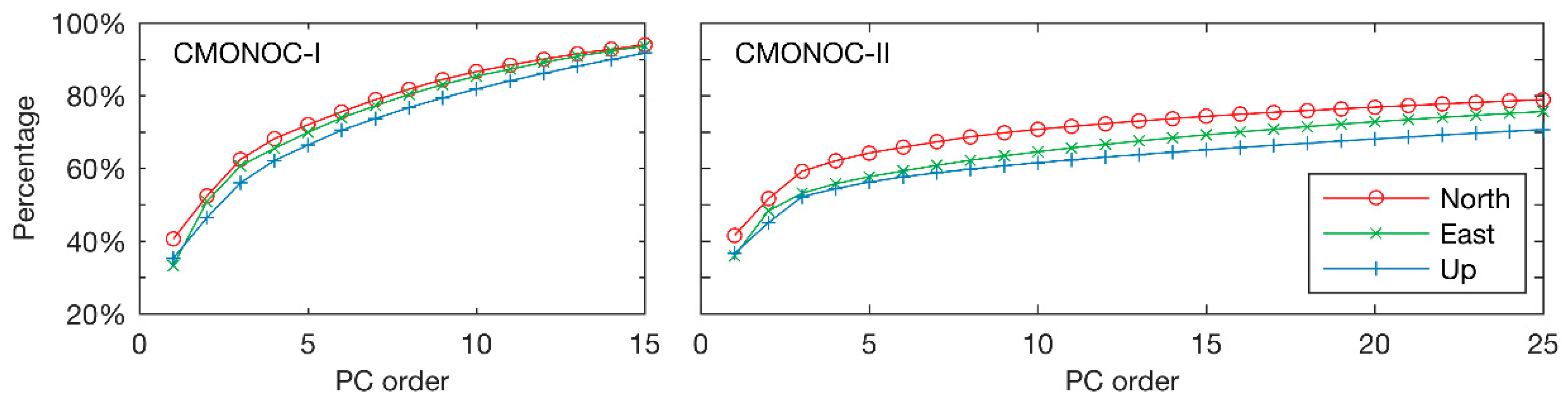
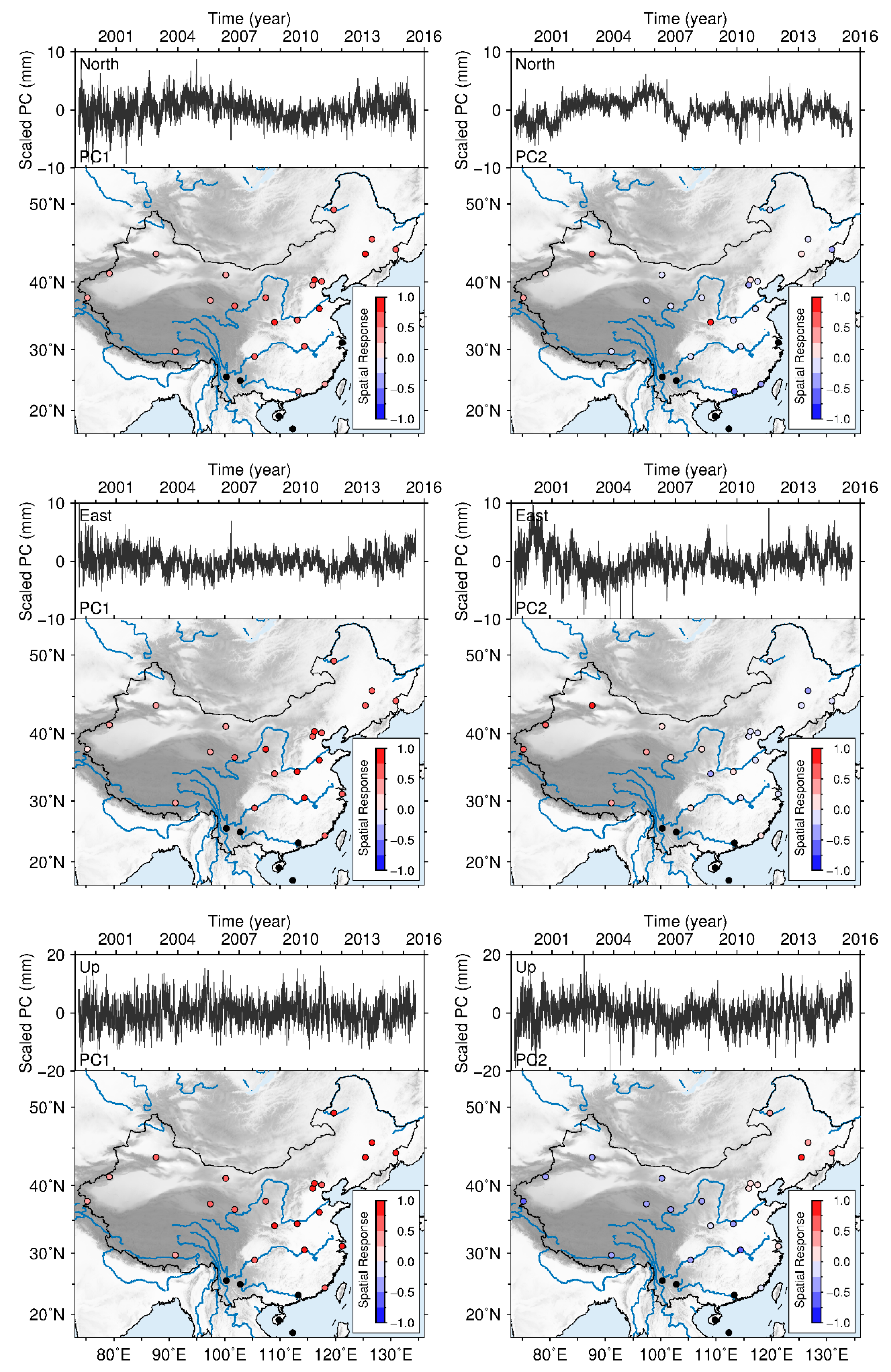
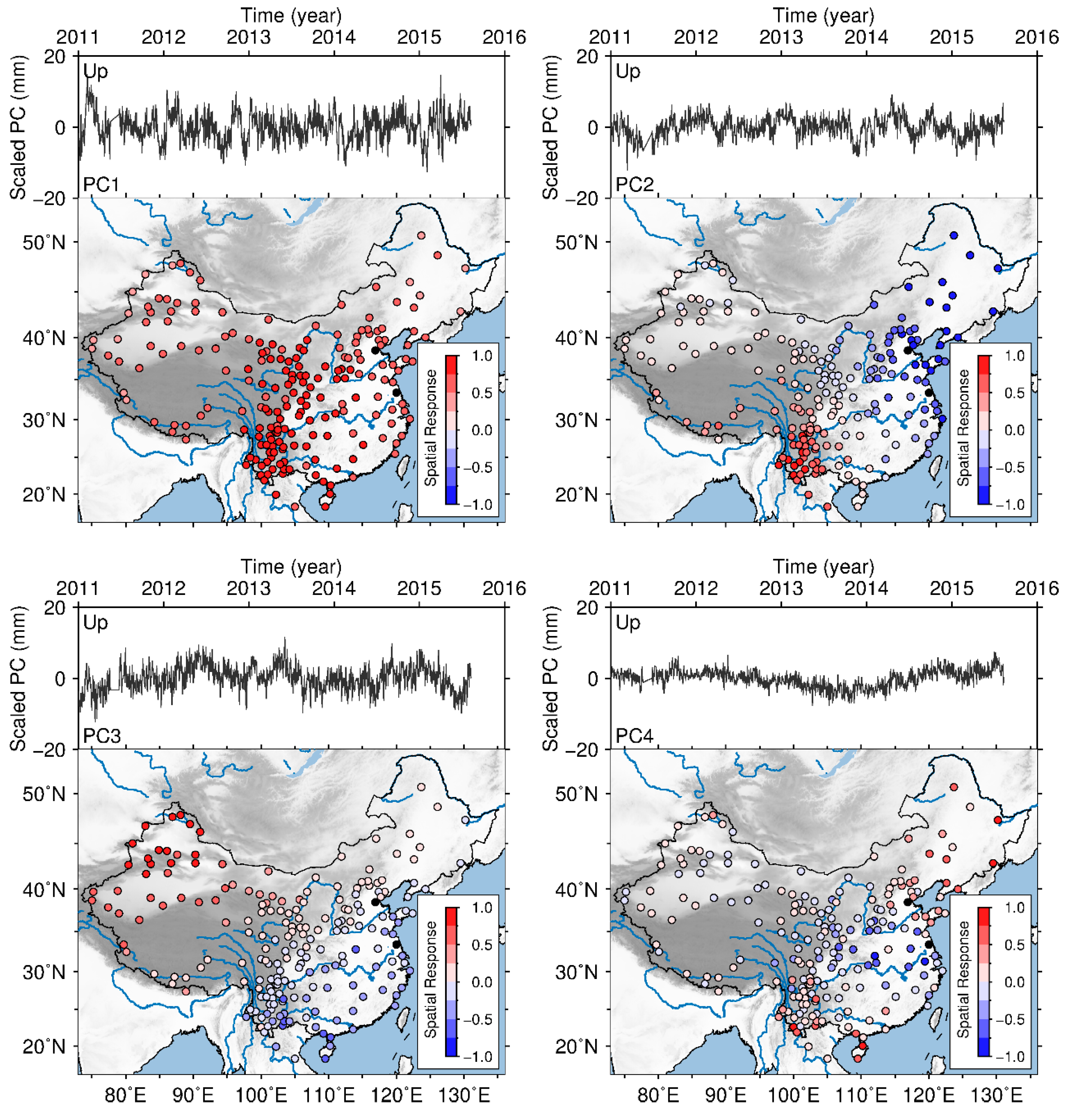
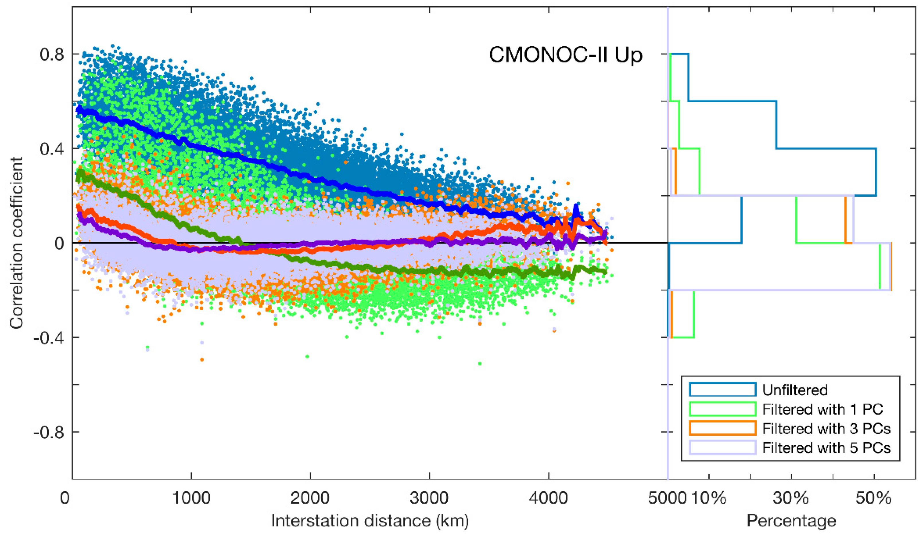
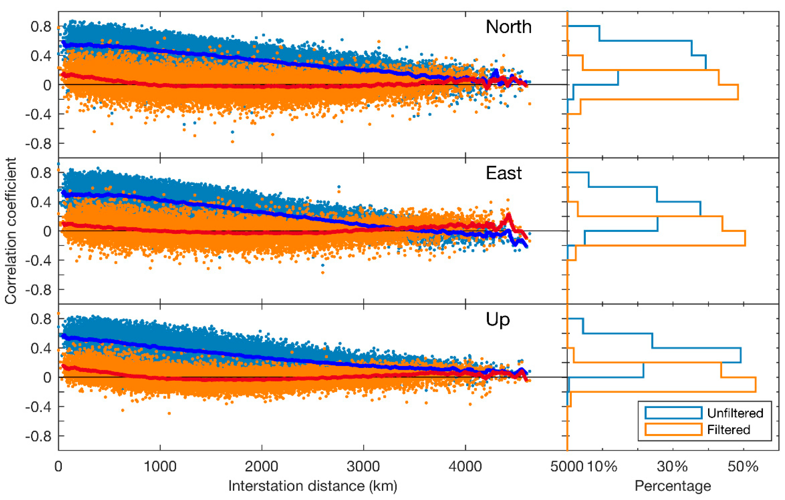
3.1. Spatial Correlation

Figure 6 illustrates the interstation correlation coefficients between the residual time series of different CMONOC stations for the unfiltered and filtered time series, respectively. The interstation correlation coefficients for the NEU components of the unfiltered time series exhibit a similar behavior: the correlation coefficients decrease gradually with increasing interstation distances and with average correlation coefficients of 0.37, 0.30 and 0.32 for the three components, respectively. Moreover, the correlation coefficients between stations can be as large as 0.8 (average value around 0.5) with interstation distance of 500 km, and then decrease to zero with an interstation distance of about 4000 km for all the three components. These results validate the existence of spatial correlation in the unfiltered residual time series for all three component time series, which is consistent with other regional GPS networks, such as in Mexico [29] and also in China [57].
After CMC filtering with PCA, the average correlation coefficients are only 0.1 for short interstation distances (tens of kilometers), and reduce to zero rapidly with interstation distances of about 700 km for all the three components. That is to say, some local scale errors still remain in the filtered time series as we conservatively adopted only the first several PCs to represent the regional CMC. However, the significant reduction of the interstation correlation coefficients indicates that PCA is an effective filtering technique for suppressing the CMC in such a large regional GPS network and the criteria for choosing significant PCs used in this paper are appropriate.

3.2. Periodic Signal

By investigating and comparing the periodic signals in the unfiltered and filtered time series, we address several questions in this section. For instance, which periodic signals (e.g., the draconitic signal) are significant in the CMONOC time series? Do these signals contribute to the CMC? Is the draconitic signal spatially correlated in the CMONOC network? As the significant difference of observing time span between CMONOC-I (≈16.5 years) and CMONOC-II (≈4.6 years) may lead to different resolutions in detecting periodic signals, these two subnetworks are treated separately. Firstly, the power spectra of each time series was generated by Lomb-Scargle periodogram technique [58,59] with an oversampling factor of 4 [60]. Then, the spectra for the NEU components of the unfiltered and filtered CMONOC-I stations were stacked respectively. Similarly, the spectra for the NEU components of the unfiltered and filtered CMONOC-II stations were stacked, respectively. These so-called stacked power spectra were also adopted by [10,13,16] to detect anomalous periodic signals in GPS position time series.
In theory, if two periodic signals (with periods of T1 and T2, respectively, and T1 > T2) are to be distinguishable, the time span of the time series must be no shorter than T1T2/(T1−T2), according to the Rayleigh criterion [61]. In reality, longer time series may be needed due to the noise in the observations [12]. Thus, at least 25.4 years are needed to distinguish the annual and draconitic signals, which exceeds the time span of our GPS observations. Nevertheless, the CMONOC-I time series can distinguish the annual and draconitic signals from their second and higher harmonics (at least 12.7 years is needed) The CMONOC-II time series can distinguish from their 6th and higher harmonics (at least 4.2 years are needed).
Figure 7 shows the stacked power spectra of the unfiltered and filtered CMONOC-I residual time series with annual and semi-annual signals removed. The slopes of the stacked spectra in the log-log plot (equal to the spectral index κ) are close to −1 (FN, κ = 1 ) at low frequencies and close to 0 (WN, κ = 0 ) at high frequencies indicating a FN + WN character on average. To focus on the draconitic harmonics and some other periodic signals, a zoom-in of Figure 7 is shown in Figure 8. Peaks at the frequencies of the annual harmonics can be seen at the third annual harmonics for all the three components, but not visible for its higher harmonics. However, significant peaks at the frequencies of the first eight draconitic harmonics are clearly visible. Moreover, peaks can also be found at the frequencies of some other draconitic harmonics, such as the 10th for the up component and the 11th, 12th, and 14th for the north component. In addition, peaks are obvious at the frequencies of 24.75, 25.74, and 26.74 cpy, equal to periods of 14.76, 14.19, and 13.66 days, for all the three components (except the 25.74 cpy for the north component). These signals are likely to be the spurious long-period signals caused by the aliasing effects of the unmodeled short-period tidal signals (diurnal O1 tide and semidiurnal M2 tide) [11,62]. The 13.66-day period spectra might also be related to the semi-monthly Mf tide. As for the filtered solution, several peaks at the frequencies of the draconitic harmonics are reduced in their stacked spectra, especially at the frequencies of the 6th draconitic harmonic for the north and east components and at the frequencies of the 8th draconitic harmonic for the up component. Moreover, the peaks at the frequencies of the 7th and 10th draconitic harmonics for the up component even become insignificant. In addition, the tri-annual signal and the periodic signals with frequencies of 24.75, 25.74, and 26.74 cpy are also reduced. Furthermore, some unknown signals are also reduced significantly, such as 3.32 cpy for the up component and 3.26 and 4.42 cpy for the north component. These unknown signals will be investigated in our future work.
Figure 9 shows the stacked power spectra of the CMONOC-II residual time series. Similar to CMONOC-I, the behavior of all the three components of CMONOC-II’s spectra follows like FN at low frequencies and like WN at high frequencies. Several peaks at the frequencies of the draconitic harmonics can also be seen but with broader bands. A zoom-in of Figure 9 is also shown in Figure 10. As the time span of the CMONOC-II is ≈4.6 years, the annual and draconitic signals can only be distinguished from their 6th harmonic onwards in theory. Thus, the broad peaks for the third to 5th draconitic harmonics are surely leaked by the corresponding annual harmonics. Moreover, only peaks at the 6th, 8th, 12th, and 14th draconitic harmonics for the north component, 6th to 9th draconitic harmonics for the east component, and 6th draconitic harmonics for the up component are identified to be caused by the draconitic signal. Moreover, the stacked power spectra of the filtered CMONOC-II time series show that the peaks are reduced significantly around the frequencies of the annual and draconitic harmonics, and only the peaks at the frequencies of 6th to 9th draconitic harmonics are still distinguishable. Moreover, the signals with frequencies of 24.75 cpy for the north and up components, and frequency of 25.74 cpy for the east component are also reduced significantly.

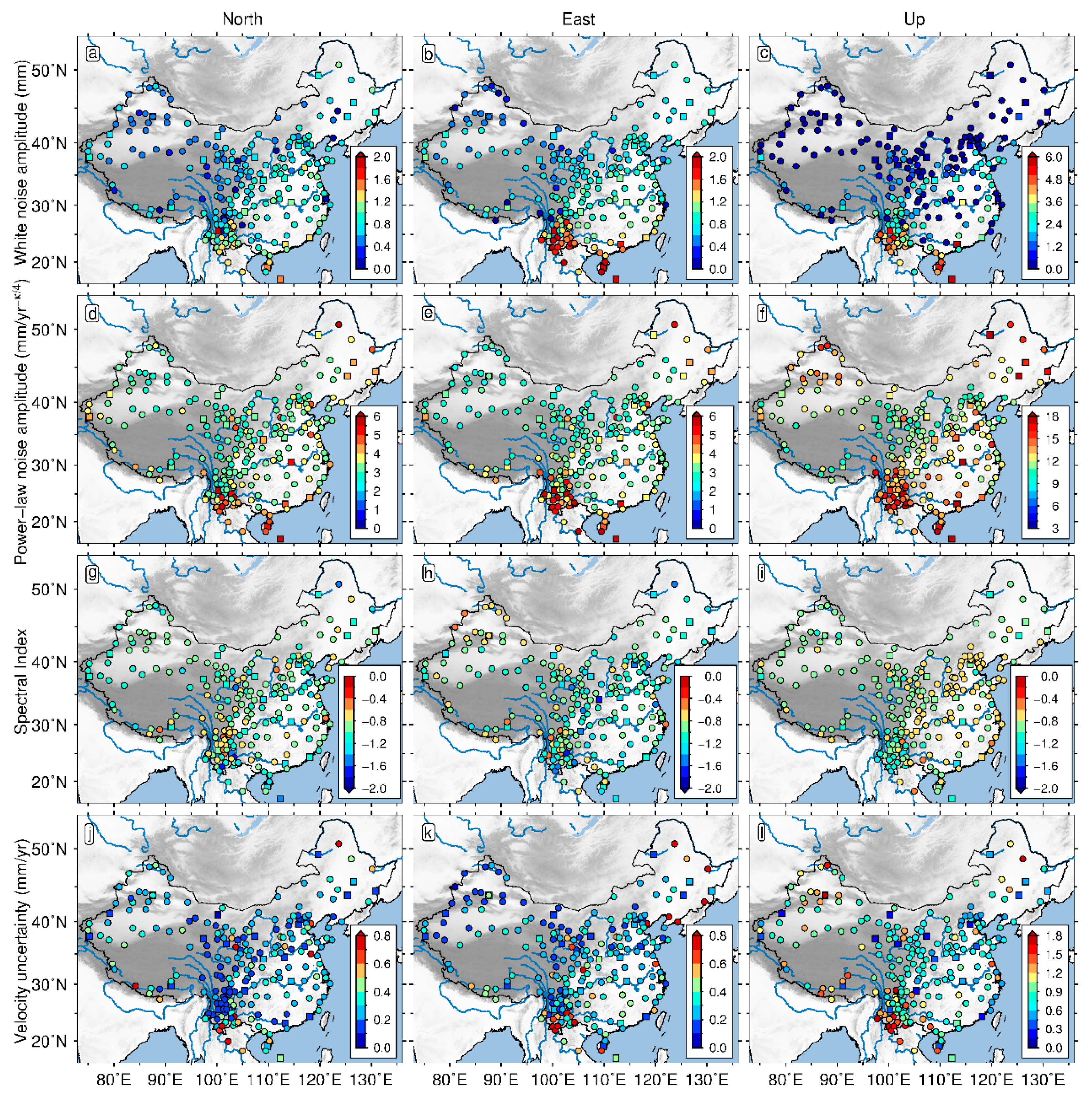
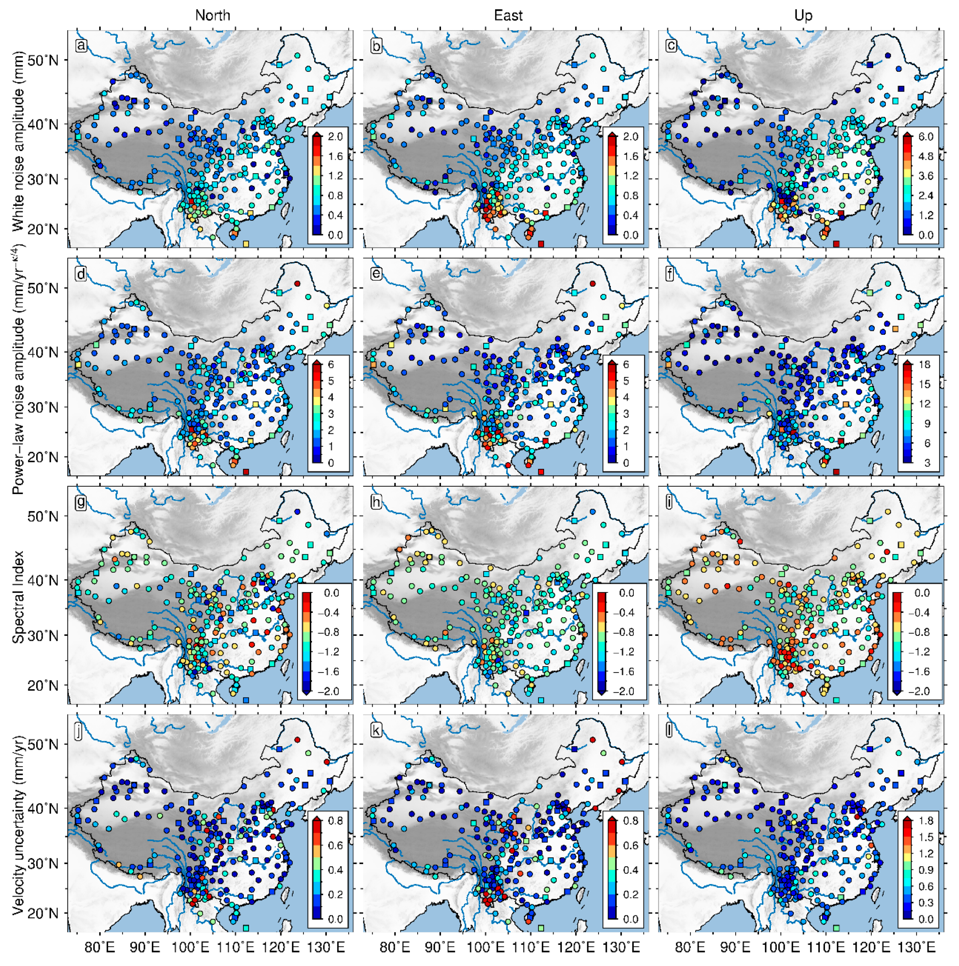
3.3. Noise Characteristics

To investigate the effects of CMC filtering on the noise characteristics of CMONOC time series, the Hector software (Ver. 1.7, http://segal.ubi.pt/hector/) with MLE was employed. Hector is a fast GPS position time series analysis software developed by Bos et al. [22] to meet the urgent demands of noise characterization for the rapidly increasing numbers of GPS stations and the accumulated GPS observations in recent years. A combination noise model of the PLN + WN is used as it is able to offer detailed description of the noise characteristics with the spectral index being estimated. Moreover, since CMONOC-I and CMONOC-II have significantly different observing time spans, they are investigated separately in this section.
Figure 11 illustrates the spatial distribution characteristics of the WN amplitudes, PLN amplitudes, spectral indices and velocity uncertainties of the unfiltered time series estimated with the PLN + WN model. The WN amplitudes of all the three components increase from north to south and reach their maximums at the southernmost China, indicating a general latitude dependence, which is consistent with [19,20]. However, the latitude dependence is not obvious for the PLN amplitudes, spectral indices and velocity uncertainties, though there are several scattered southern stations with extraordinary large values. In addition, the WN amplitudes generally vary up to 2 mm and up to 6 mm for the horizontal and vertical components, respectively. The PLN amplitudes generally vary from 2 to 6 mm/yearκ/4 and from 6 to 18 mm/yearκ/4 for the horizontal and vertical components, respectively. The spectral indices are generally from −0.6 to −1.6 for the horizontal and from −0.6 to −1.2 for vertical components, respectively. The velocity uncertainties generally vary up to 0.8 mm/year and up to 2.4 mm/year for the horizontal and vertical components, respectively.
As a comparison, Figure 12 illustrates the spatial distribution characteristics of the WN amplitudes, PLN amplitudes, spectral indices and velocity uncertainties of the filtered time series estimated with the PLN + WN model. After CMC filtering, the PLN amplitudes and velocity uncertainties are generally reduced significantly. However, some stations in Yunnan province (between longitude 97°E–107°E and latitude 20°N–30°N) still show significant PLN amplitudes and velocity uncertainties. Most of these stations are excluded from the calculation of CMC because of their abnormal non-linear variations and just filtered with the average CMC of the network. Their abnormal non-linear variations might be related to the droughts that occurred in Yunnan [8].
Table 1 lists the mean and standard deviations of the WN amplitudes, PLN amplitudes, spectral indices, velocity uncertainties, and RMS of the CMONOC-I time series before and after CMC filtering. After the filtering, the average WN amplitudes are slightly reduced in horizontal but enlarged in the vertical direction, indicating that the WN component is probably correlated to site-specific errors that cannot be removed by CMC filtering. Nevertheless, their average PLN amplitudes show significant reductions for all the three components of the filtered time series, with average reduction ratios of 27%, 20%, and 27% for the NEU components, respectively. Moreover, the average spectral indices are slightly reduced for the north and up components. As for the velocity uncertainty estimates, they are reduced by 4%, 18%, and 16% on average for the NEU components, respectively, Furthermore, obvious RMS reductions can also be noticed from Table 1, indicating an improved signal-to-noise ratio.
Table 2 lists the mean and standard deviations of the WN amplitudes, PLN amplitudes, spectral indices, velocity uncertainties and RMS of the CMONOC-II time series before and after CMC filtering. The average WN amplitudes are also slightly reduced in horizontal but enlarged in vertical after the filtering, which are similar to the changes of WN amplitudes for the CMONOC-I time series. However, compared with the reduction ratios of CMONOC-I stations’ PLN amplitude, the CMONOC-II stations’ PLN amplitude show much larger reductions for all the three components after CMC filtering, with average reduction ratios of 47%, 46%, and 52% for the NEU components, respectively. Moreover, the CMONOC-II stations’ velocity uncertainty estimates also obtain greater reduction ratios after CMC filtering, with average reduction ratios of 33%, 38%, and 54% for the NEU components, respectively.
To quantitatively estimate the effects of the filtering on geophysical parameters, we compare the station velocities between the filtered and unfiltered time series estimated with the PLN + WN model. Their differences are displayed in Figure 13. The majority of the differences are within ±0.3 mm/year and within ±0.6 mm/year for the horizontal and vertical components, respectively.

4. Discussion

4.1. Characteristics of the Draconitic Harmonics

Figure 7, Figure 8, Figure 9 and Figure 10 have demonstrated that CMC filtering with PCA is capable to decrease the draconitic harmonics for both CMONOC-I and CMONOC-II. Compared with CMONOC-I, CMONOC-II shows a more significant reduction. We attribute this difference to the fact that the spatial correlations between the CMONOC-II stations are more significant as their interstation distances are much smaller and, thus, more CMC components are reduced by the filtering. In addition, a considerable part of the CMONOC-I stations are not included in the calculation of CMC and just corrected with the average responses. In general, these results indicate that the CMC in the CMONOC time series contains the draconitic harmonic and some other periodic signals, thus supporting the conclusion drawn by Amiri-Simkooei [63] and Amiri-Simkooei et al. [12] that the draconitic signal is correlated in space. However, these results cannot exclude the possibility that the draconitic signal is partly due to site-specific effects as suggested by King and Watson [16] because there are still several peaks visible at the frequencies of the draconitic harmonics and the estimation of the power spectrum has uncertainty. Moreover, these results are consistent to the conclusions of Abraha et al. [17].

4.2. Changes of the Noise Characteristics Due to CMC Filtering

In Section 3.3, the CMONOC-I and CMONOC-II time series have been analyzed with the PLN + WN, respectively. For both of the CMONOC-I and CMONOC-II, their PLN amplitudes and velocity uncertainties are reduced after CMC filtering, consistent with prior studies [31,57,64]. However, as the two subnetworks have significant differences in the time span of observations, the number of stations, and interstation distances, they may show some differences in their noise characteristics before and after CMC filtering. Before CMC filtering, the average WN amplitudes, PLN amplitudes and RMS of the CMONOC-II time series are lower than those of the CMONOC-I time series, which may be due to the fact that the quality of the latest observations are better than the early observations. While the average velocity uncertainties of the CMONOC-II time series are larger than those of the CMONOC-I time series as their time span of observations are much shorter. Comparing the effects of CMC filtering on CMONOC-I and CMONOC-II time series, one can find that the CMONOC-II time series show much larger reductions in PLN amplitude and velocity uncertainty estimates for all three components, indicating that the CMONOC-II time series benefit more from CMC filtering. This may be because that the CMONOC-II subnetwork has shorter interstation distances and the first three PCs are used for the calculation of its CMC, whereas only the first PC is used to calculate CMC of the CMONOC-I subnetwork.
Table A2 lists the velocity estimates and their uncertainties for the unfiltered and filtered NEU component time series for the CMONOC stations estimated with the PLN + WN model. Moreover, the horizontal and vertical velocity field of the CMC filtered CMONOC time series estimated with the PLN + WN model are shown in Figure 14 and Figure 15, respectively. The velocity estimates of CMONOC stations provide abundant information on the tectonic deformation over the mainland China and we will focus on it in our future work.

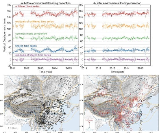
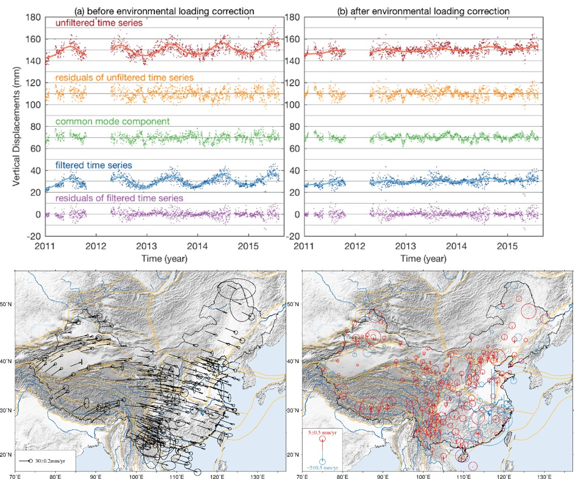
4.3. Environmental Loading Effects on the CMC

Environmental loading is one of the potential candidates for the CMC (Dong et al., 2006). In this section, the contributions of environmental loading to the CMC of the CMONOC network is quantified. As environmental loading effects are usually most significant in vertical, only the CMONOC height time series are analyzed. We firstly obtained the vertical environmental loading displacements for the CMONOC stations predicted with loading products from German Research Centre for Geosciences (GFZ) [66], in which atmospheric loading, non-tidal oceanic loading and hydrological loading effects are taken into account. Environmental loading displacements at a station are shown in Figure A6 as an example.
We then calculated and compared the RMS of CMC for the CMONOC height time series before and after environmental loading correction as shown in Figure 16a,b. RMS reduction ratios of the corresponding CMC are shown in Figure 16c. For the CMONOC height time series before and after environmental loading correction, the RMS of CMC range from 1.4 mm to 5.0 mm and from 0.3 mm to 4.7 mm with medians of 3.4 mm and 2.7 mm, respectively. In addition, the according RMS reduction ratios of CMC range between −9.1% and 77.8%, with a median of 18.4% at station Wuqia (XJWU, 39.7°N, 75.2°E). To illustrate and compare the time series before and after environmental loading correction, station XJWU is selected as an example as shown in Figure 17. Before loading correction, the RMS of station XJWU’s unfiltered and filtered height time series are 4.1 mm and 2.8 mm, respectively. After loading correction, the RMS of station XJWU’s unfiltered and filtered height time series are 3.6 mm and 2.6 mm, respectively. Accordingly, the RMS of CMC for station XJWU’s height time series decrease from 3.0 mm to 2.4 mm after the environmental loading correction.
In general, 224 of the 231 stations show a decrease in the RMS of CMC after the environmental loading correction and 170 of them are with a RMS reduction ratio of CMC larger than 10%, confirming that environmental loading is one of the sources of CMC for the CMONOC height time series, which is consistent with Zhu et al. [6].

5. Conclusions

Daily position residual time series of 231 CMONOC GPS stations have been analyzed to investigate the effects of CMC filtering with PCA on the periodic signals and noise characteristics. The source of the draconitic signal in the CMONOC GPS position time series was discussed. The noise characteristics of the CMONOC-I (27 stations, ≈16.5 years) and CMONOC-II (204 stations, ≈4.6 years) stations before and after CMC filtering have been compared, and possible reasons for their differences have been discussed, such as the differences in time span of observations, number of stations, and interstation distances. Therefore, a unified, realistic, and three-dimensional CMONOC GPS velocity field estimated with the consideration of colored noise is given. Furthermore, contributions of environmental loading to the CMC of CMONOC were quantified as well. The following are the main findings:
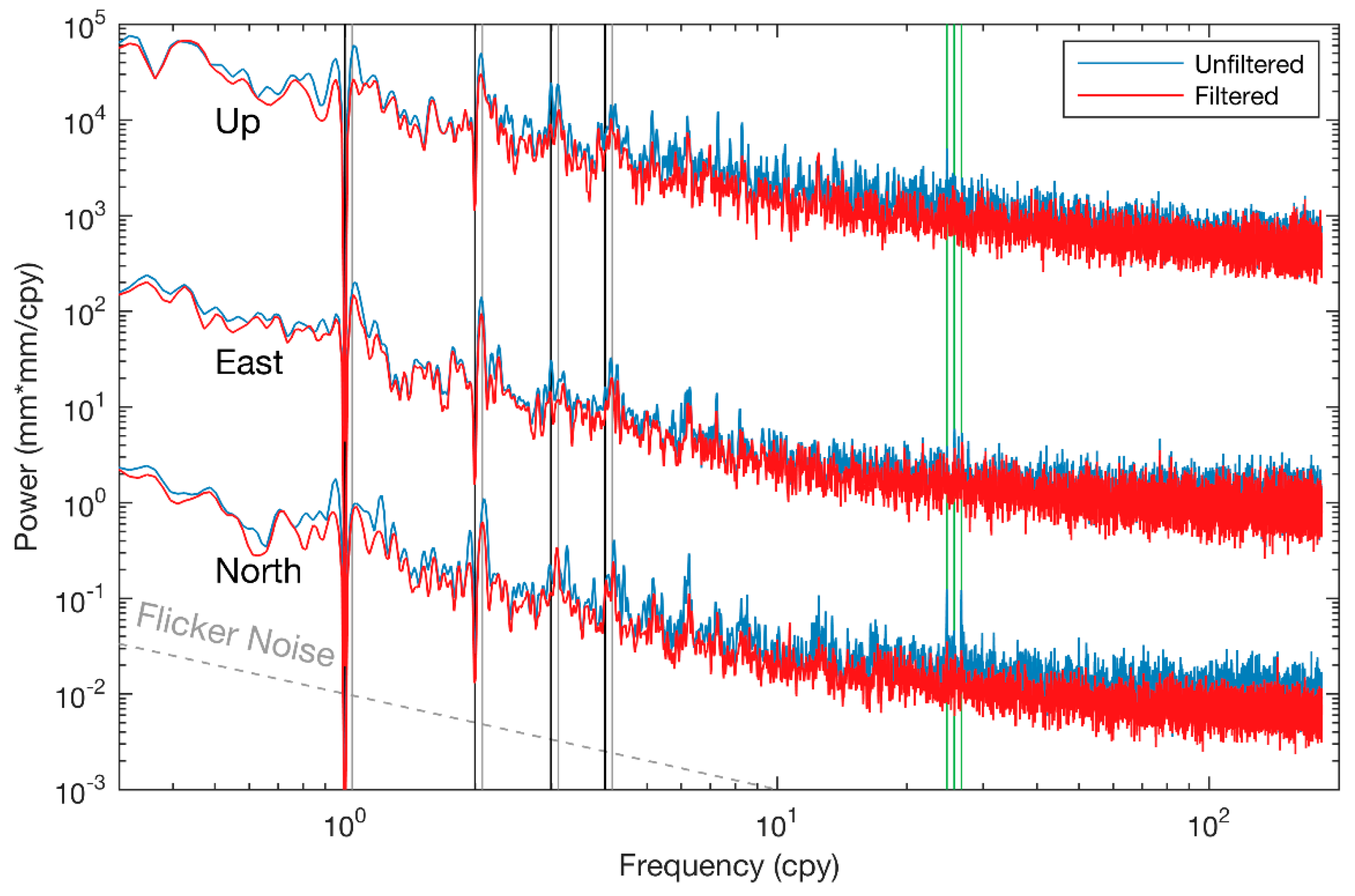
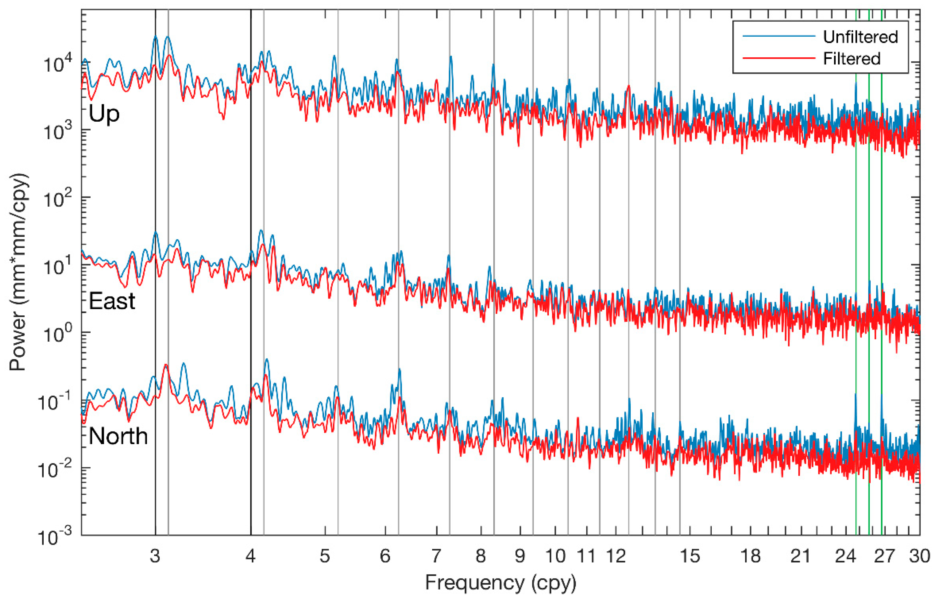
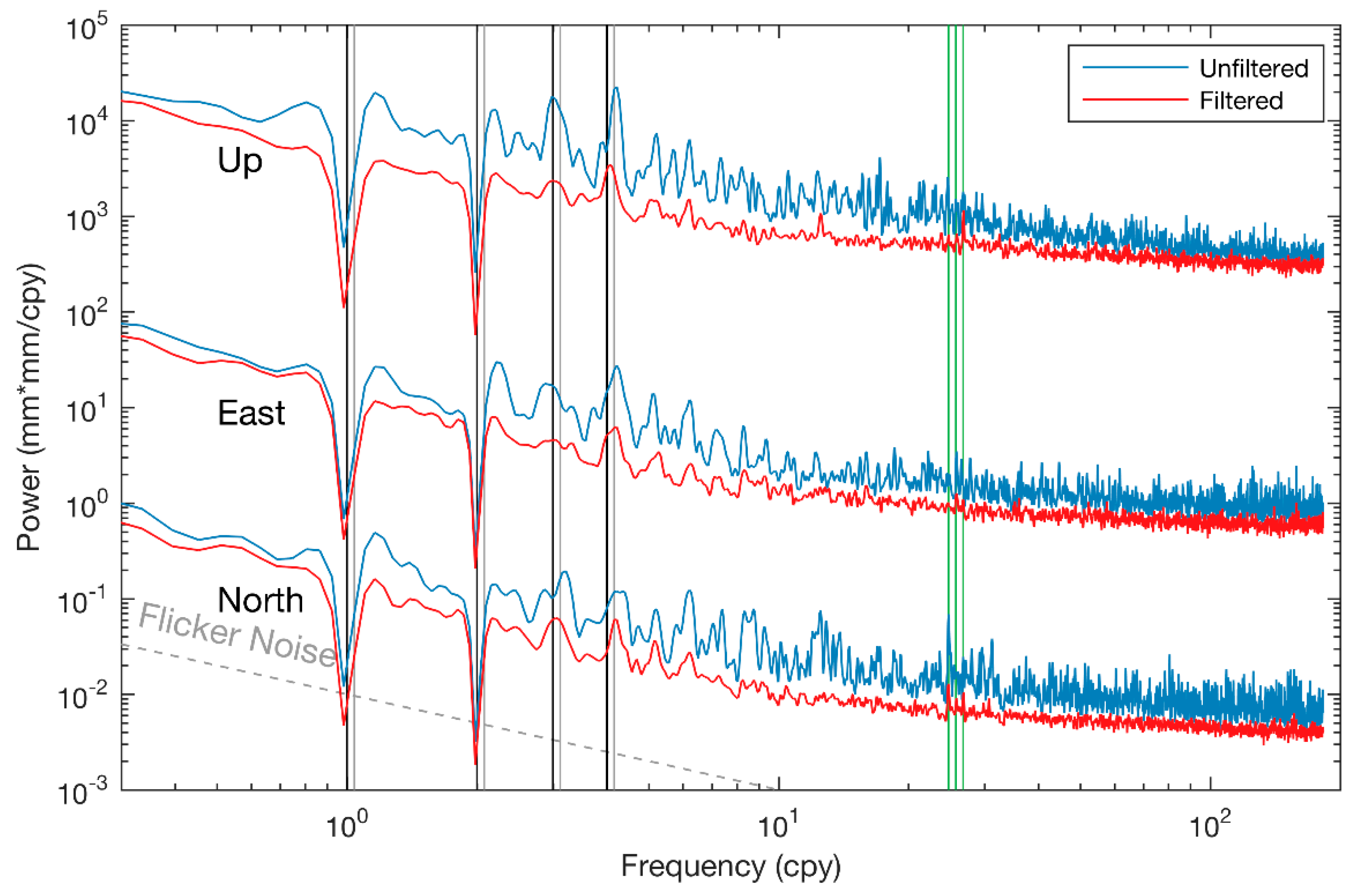
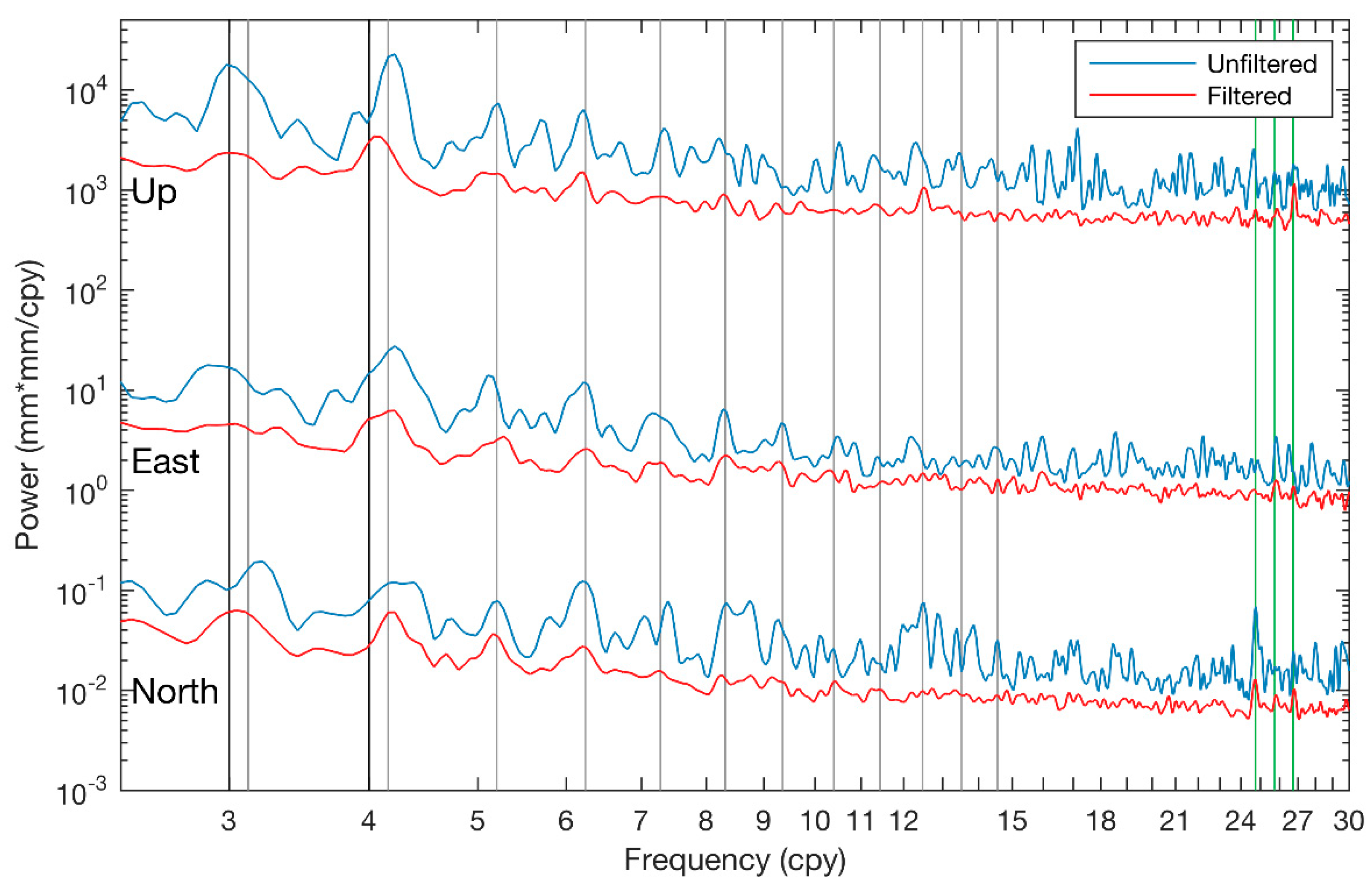
  • The stacked power spectra of the CMC-filtered CMONOC residual time series show that peaks are reduced significantly at frequencies of tri-annual, draconitic harmonics up to 14th, and 24.75, 25.74, and 26.74 cpy, indicating that the CMC of the CMONOC network contains draconitic harmonics and some other periodic signals. These results support the view that the draconitic signal is spatially correlated. However, the possibility that the draconitic signal is caused by site-specific effects cannot be ruled out because of the weakened, but still visible, peaks at the frequencies of the draconitic harmonics.
  • For the unfiltered time series, the velocity uncertainties of the CMONOC stations estimated with an assumption of the PLN + WN model generally vary up to 0.8 mm/year and up to 2.4 mm/year for the horizontal and vertical components, respectively. After CMC filtering, the average white noise amplitudes are slightly reduced in horizontal but enlarged in vertical for both the CMONOC-I (≈16.5 years) and CMONOC-II (≈4.6 years) stations. Nevertheless, the average power-law noise amplitudes are significantly suppressed by CMC filtering. Therefore, the velocity uncertainty estimates of north, east and up components for both the CMONOC-I and CMONOC-II stations are reduced. Compared with CMONOC-I, the CMONOC-II stations obtain greater reduction ratios in velocity uncertainty estimates with average values of 33%, 38%, and 54% for the north, east, and up components, respectively. These results indicate that CMC filtering can suppress the colored noise amplitudes and improve the precision of velocity estimates.
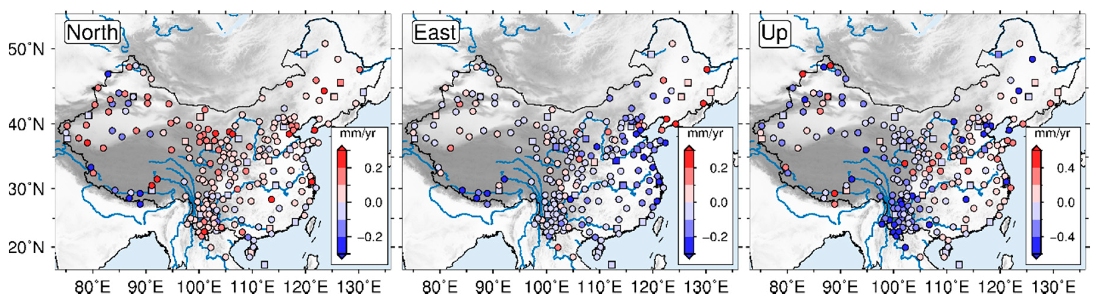
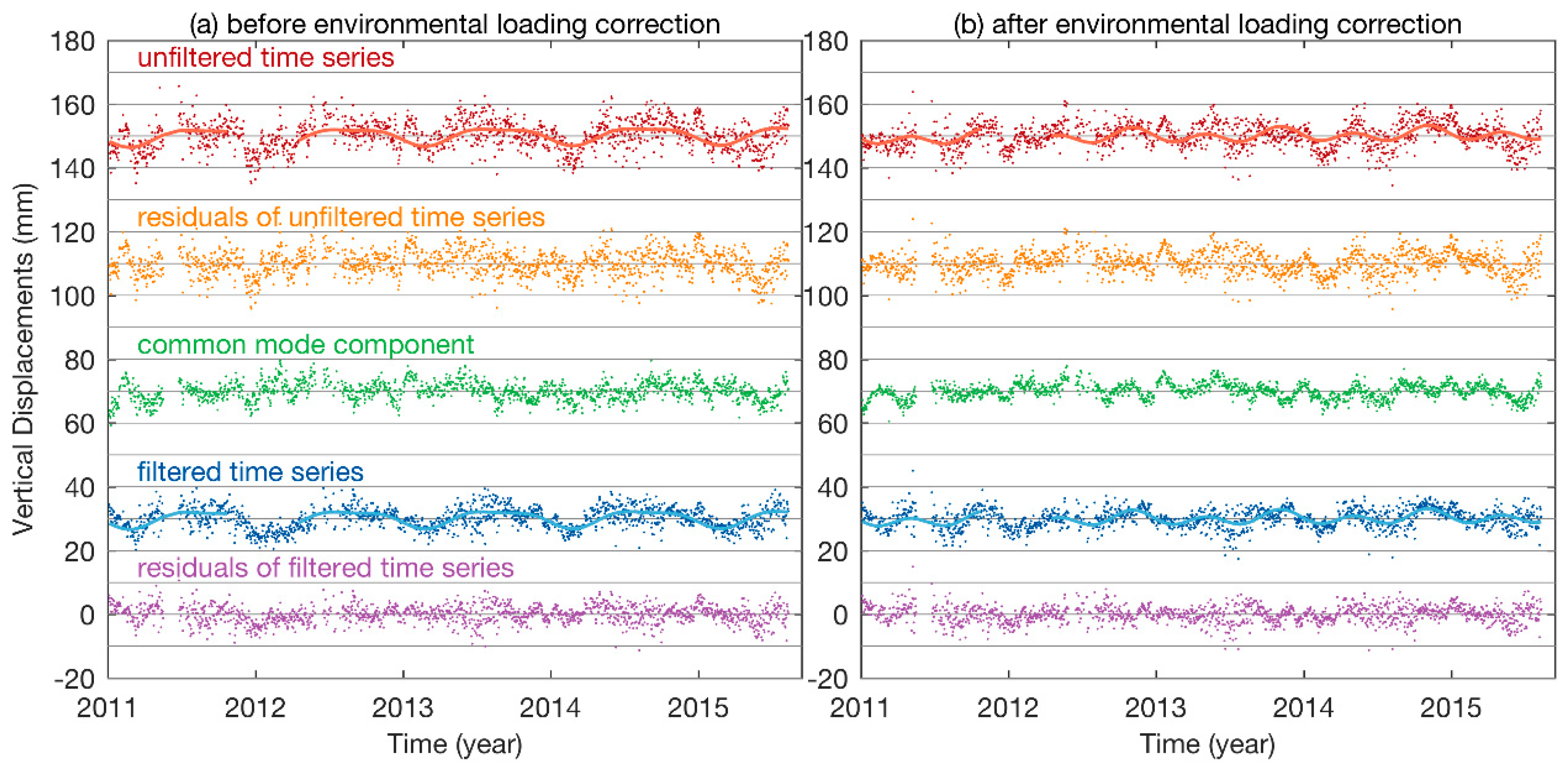
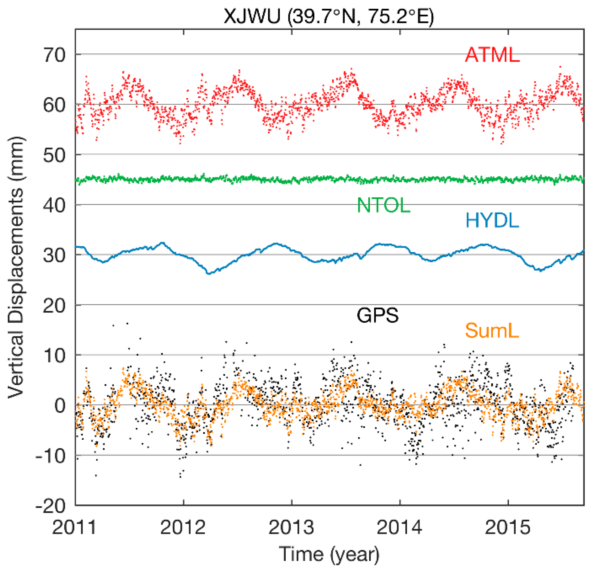
  • After environmental loading correction, vertical CMC are reduced at 224 of the 231 CMONOC stations. In addition, 170 of them are with an RMS reduction ratio of CMC larger than 10%, confirming that environmental loading is one of the sources of CMC for the CMONOC height time series.

Author Contributions

P.Y. and W.J. conceived and designed the experiments; P.Y. performed the experiments; P.Y. and K.W. analyzed the data; W.J. and N.S. gave critical suggestions and amendments. P.Y. wrote the main manuscript text, and the other authors helped with the writing of the text.

Funding

This research was funded by the National Science Fund for Distinguished Young Scholars of China (grant no. 41525014), the Science Fund for Creative Research Groups of the National Natural Science Foundation of China (grant no. 41721003), the Program for Changjiang Scholars of the Ministry of Education of China and the Major Project of Beijing Future Urban Design Innovation Center, Beijing University of Civil Engineering and Architecture (UDC 2018031321). German Academic Exchange Service (DAAD) Thematic Network Program “Modern Geodetic Space Techniques for Global Change Monitoring” (Project ID. 57173947).

Acknowledgments

We are grateful to IGS WHU (http://www.igs.gnsswhu.cn/) and CMONOC (http://neiscn.org/chinsoftdmds/ltwl/) for providing the GPS data, MIT for providing the GAMIT/GLOBK software (version 10.5, http://geoweb.mit.edu/gg/), Machiel Bos, Rui Fernandes and Luisa Bastos for providing the Hector software (version 1.7, http://segal.ubi.pt/hector/), GFZ for providing the environmental loading products (https://isdc.gfz-potsdam.de/esmdata/loading/), and the Global CMT Catalog Search for providing the earthquake information (http://www.globalcmt.org/CMTsearch.html). In this paper, the figures with geographical maps were generated with the Generic Mapping Tools (version 5.3.1, http://gmt.soest.hawaii.edu/) and all the other figures were generated with MATLAB (version R2017b, https://www.mathworks.com/products/matlab.html).

Conflicts of Interest

The authors declare no conflict of interest.

Appendix A

Figure A1. Location map of the globally distributed 73 IGS stations which are generally selected from the core network of IGb08 reference frame (ftp://igs.org/pub/station/coord/IGb08_core.txt). The black and blue dots indicate two subnetwork stations, respectively. The red pentagrams indicate the common stations of these two subnetworks.
Remotesensing 10 01472 g0a1
Figure A2. An example of stations affected by co- and post-seismic deformation. Station Hegang (HLHG) is located in Northeast China and about 1500 km away from the epicenter (red solid circle) of the Mw 9.0 Tohoku-Oki Earthquake. The gray curve indicate the fitting curve of east component modeled with Equation (1). The black curves indicate the fitting curves of the NEU components modeled with Equation (1), but without the logarithmic term. The post-seismic deformation is not significant for north or up components of HLHG and, thus, there is no need to be taken into consideration in the function model. As for the east component of HLHG, obvious post-seismic deformation can be noticed and, thus, a logarithmic term needs to be included in the function model.
Remotesensing 10 01472 g0a2
Figure A3. Same as Figure 4, but for the north component.
Remotesensing 10 01472 g0a3
Figure A4. Same as Figure 4, but for the east component.
Remotesensing 10 01472 g0a4
Figure A5. Unfiltered time series (red, shifted upward by 150 mm) and their residual time series (orange, shifted upward by 110 mm) obtained with Equation (1), common mode error (green, shifted upward by 70 mm), and filtered time series (blue, shifted upward by 30 mm), and their residual time series (purple) obtained with Equation (1) for the selected three vertical position time series of the CMONOC-II stations, in which station XJML, HAHB and HECX are characterized by the maximum, medium and minimum RMS reduction in CMONOC-II after the filtering, respectively.
Remotesensing 10 01472 g0a5
Figure A6. Vertical displacement time series due to atmospheric loading (ATML, red), non-tidal oceanic loading (NTOL, green), hydrological loading (HYDL, blue), and their summation (SumL, orange) predicted with GFZ loading products and GPS height time series (black) for station XJWU. The ATML, NTOL, and HYDL time series are shifted upward by 60, 45, and 30 mm, respectively.
Remotesensing 10 01472 g0a6
Table A1. The earthquakes which caused co-seismic and/or post-seismic deformation of the CMONOC stations (http://www.globalcmt.org/CMTsearch.html [51,52]).
Time
(Greenwich Mean Time)
EpicenterMagnitude (Mw)
Longitude (°)Latitude (°)Region
20 September 1999120.824.2Nantou, Taiwan, China7.6
14 November 200192.935.8Kokoxili, Qinghai, China7.8
26 December 200494.33.1Indian Ocean9.0
8 October 200573.534.4Pakistan7.6
12 May 2008104.131.4Wenchuan, Sichuan, China7.9
6 October 200890.529.7Dangxiong, Xizang, China6.3
11 March 2011143.137.5Tohoku-Oki, Japan9.1
20 April 2013103.130.2Lushan, Sichuan, China6.6
21 July 2013104.334.6Minxian, Gansu, China6.0
12 February 201482.636.2Yutian, Xinjiang, China6.9
25 April 201585.327.9Nepal7.9
12 May 201586.127.7Nepal7.2
Table A2. Three-dimensional velocity estimates and their uncertainties of the CMC filtered 231 CMONOC stations estimated with the PLN + WN model. The reference frame is IGb08.
StationLat. (°)Lon. (°)Velocity (mm/year)Velocity Uncertainty (mm/year)
NEUNEU
AHAQ117.030.6−11.1733.030.720.060.070.36
AHBB117.332.9−10.7832.790.180.100.060.40
BJFS115.939.6−10.6930.201.830.240.180.16
BJGB117.240.7−10.4829.781.570.050.050.23
BJSH116.240.3−11.2829.550.820.090.070.15
BJYQ116.040.4−10.5930.661.140.090.060.19
CHUN125.443.8−11.7725.890.270.120.140.45
CQCS107.229.9−9.1534.680.270.090.170.19
DLHA97.437.41.0337.230.700.150.320.23
DXIN100.241.0−4.5830.721.150.130.100.18
FJPT119.825.5−11.7131.220.400.300.470.28
FJWY118.027.6−11.5033.030.930.160.140.47
FJXP120.026.9−11.4632.961.060.080.150.23
GDSG113.624.8−10.5933.60−0.060.110.440.57
GDZH113.622.3−11.1833.685.750.070.090.40
GDZJ110.321.2−10.5033.672.060.200.230.40
GSAX95.840.5−0.2431.270.210.120.090.13
GSDH94.740.10.4830.81−0.010.170.260.19
GSDX104.635.6−6.6936.400.680.060.040.19
GSGL102.937.5−4.7834.371.960.450.481.07
GSGT99.839.4−3.3831.611.240.090.080.18
GSJN105.835.5−8.4934.680.670.180.080.44
GSJT104.137.2−5.2934.751.090.080.250.13
GSJY98.239.8−1.9331.512.020.170.160.19
GSLX104.635.0−7.0135.520.910.100.110.26
GSLZ103.736.1−0.7540.94−2.661.750.750.23
GSMA102.134.0−4.2541.411.310.350.130.27
GSML100.838.4−2.9233.020.680.110.120.19
GSMQ103.138.6−5.5032.48−0.300.370.060.71
GSMX104.034.4−5.9238.080.830.120.140.36
GSPL106.635.5−8.9535.061.040.050.610.48
GSQS106.234.7−7.7133.770.340.220.200.37
GSWD104.833.4−8.1536.17−0.240.390.310.50
GUAN113.323.2−11.0332.640.550.200.320.97
GXBH109.221.7−8.4133.302.200.310.140.45
GXBS106.723.9−9.0734.60−1.070.160.120.65
GXHC108.024.7−9.3034.541.070.080.110.36
GXNN108.122.6−9.2233.852.070.140.090.55
GXWZ111.223.5−9.4334.24−1.570.160.160.47
GZFG107.728.0−9.4233.321.890.370.600.82
GZGY106.726.5−9.0134.940.370.050.200.70
GZSC104.926.6−8.7334.681.460.080.100.31
HAHB114.535.7−10.8132.43−0.540.060.090.42
HAJY112.435.2−10.3533.140.190.150.090.56
HAQS114.032.8−10.6134.24−1.640.040.080.40
HBES109.530.3−9.9934.101.940.190.110.81
HBJM112.231.1−10.7334.770.830.190.340.38
HBXF112.032.0−10.4833.691.200.100.060.58
HBZG111.030.8−9.2634.570.100.470.440.49
HECC115.840.9−10.6429.851.280.100.050.21
HECD117.941.0−9.8529.810.710.080.120.36
HECX116.938.5−9.7430.82−24.120.430.382.34
HELQ114.338.2−10.4832.114.240.080.140.49
HELY114.737.4−10.3733.231.170.200.140.25
HETS118.339.7−6.3327.702.390.770.891.43
HEYY114.240.1−10.9032.471.010.120.390.31
HEZJ114.940.8−9.9130.082.050.340.190.29
HIHK110.220.0−10.4333.02−1.250.370.130.57
HISY109.518.2−8.1534.072.680.260.630.75
HLAR119.749.3−11.3225.791.440.100.090.30
HLHG130.247.4−15.9024.380.290.781.450.54
HLWD126.148.7−12.2425.210.250.440.410.83
HNLY113.628.2−10.3533.720.030.080.080.59
HNMY109.827.9−9.7134.510.680.060.200.29
HRBN126.645.7−11.7624.98−0.450.160.180.21
JIXN117.540.1−10.1228.171.740.120.060.17
JLCL123.544.6−11.6228.38−0.550.260.230.35
JLYJ129.542.9−16.8126.47−0.110.320.700.44
JSLS119.431.3−11.3933.56−1.920.270.121.14
JSLY119.534.7−12.0532.060.470.060.080.26
JSNT120.932.0−11.7832.83−1.330.100.130.31
JSYC120.033.4−9.7632.46−11.280.440.271.46
JXJA115.126.7−11.1333.93−0.440.060.310.37
KMIN102.825.0−16.7333.53−1.670.390.970.75
LALB102.219.9−6.2531.402.230.400.280.34
LALX105.018.2−8.7431.522.680.400.440.47
LHAS91.129.715.5046.661.790.120.150.38
LNDD124.340.0−10.6826.090.130.271.120.37
LNJZ121.739.1−12.0329.420.630.290.110.42
LNYK122.640.7−11.6427.761.200.120.260.31
LUZH105.428.9−9.5634.650.730.100.190.12
NMAG122.643.3−11.0028.741.670.100.150.33
NMAL120.143.9−10.9228.741.200.120.100.36
NMAY101.739.2−5.2531.821.510.230.050.12
NMAZ105.738.8−6.6331.840.920.260.210.33
NMDW117.045.5−10.5328.40−0.240.120.080.29
NMEJ101.142.0−4.5031.411.120.230.030.26
NMEL111.943.6−9.6129.521.700.170.300.17
NMER123.750.6−11.2825.120.711.921.370.50
NMTK111.340.3−10.5731.581.610.180.400.41
NMWH106.839.7−9.6232.423.750.120.190.29
NMWJ108.141.3−9.4330.090.860.120.270.29
NMWL122.046.0−10.9627.571.120.170.170.56
NMZL116.042.2−10.2029.601.330.280.030.20
NXHY105.636.6−6.5534.59−0.930.100.150.18
NXYC106.338.5−7.3432.04−4.250.680.620.49
NXZW105.237.6−5.6233.251.520.050.130.16
QHBM100.732.9−4.9444.901.020.070.050.18
QHDL98.136.32.5338.020.580.080.110.27
QHGC100.137.3−2.1037.580.630.140.070.34
QHGE94.836.14.5337.160.200.140.130.65
QHLH93.338.73.1234.622.860.500.150.38
QHMD98.234.90.5045.521.620.070.090.42
QHME101.437.5−3.1237.091.350.100.140.40
QHMQ100.234.5−1.1242.300.510.170.050.22
QHMY90.838.57.1635.511.060.140.070.22
QHQL100.238.2−3.1334.701.670.150.340.30
QION109.819.0−10.9331.640.390.200.150.28
SCBZ106.731.8−9.1334.331.210.040.060.20
SCDF101.131.0−12.2543.381.600.090.480.33
SCGY105.932.4−8.3334.560.580.190.790.38
SCGZ100.031.6−9.3047.06−0.600.110.420.33
SCJL101.529.0−17.8239.772.030.100.060.52
SCJU104.528.2−7.6134.730.510.170.270.84
SCLH100.731.4−11.0946.191.160.060.190.28
SCMB103.528.8−8.9935.250.220.130.210.32
SCML101.327.9−19.4948.87−2.910.070.240.39
SCMN102.228.3−16.2939.100.320.050.090.20
SCMX103.831.7−6.4845.069.280.240.310.34
SCNC105.931.0−9.5834.821.280.100.190.12
SCNN102.727.1−16.3437.930.670.610.360.27
SCPZ101.726.5−17.8036.011.060.090.080.15
SCSM102.429.2−12.1938.081.860.050.060.34
SCSN105.630.5−8.8334.301.500.040.110.21
SCSP103.632.6−10.0341.081.430.140.150.34
SCTQ102.830.1−9.6635.942.920.180.290.45
SCXC99.828.9−16.9941.522.820.050.120.34
SCXD102.428.3−14.1538.710.170.040.090.19
SCXJ102.431.0−6.0540.860.300.350.240.19
SCYX102.528.7−13.0938.12−0.910.130.160.30
SCYY101.527.4−17.6038.620.800.100.100.16
SDCY119.536.8−11.4631.381.840.110.070.47
SDJX116.435.4−11.0632.741.820.130.080.30
SDLY118.335.0−12.4231.712.720.940.280.70
SDQD120.336.1−11.3431.781.240.050.050.19
SDRC122.437.2−11.3831.25−2.270.100.140.65
SDYT121.437.5−10.9630.290.680.170.070.18
SDZB118.036.8−11.2832.240.920.270.170.42
SHA2121.231.1−11.7731.93−1.550.150.170.48
SHAO121.231.1−13.3232.16−1.910.250.240.27
SNAK108.832.8−9.8134.621.450.250.280.40
SNMX106.733.1−10.5735.06−1.390.680.280.82
SNTB107.334.1−9.6035.281.060.060.100.43
SNXY108.435.2−9.2734.181.280.060.060.37
SNYA109.536.6−10.4732.082.160.120.590.27
SUIY130.944.4−12.4924.52−1.140.110.180.40
SXCZ113.236.2−9.5830.041.340.250.290.23
SXGX111.936.3−9.6932.543.020.360.100.61
SXKL111.638.8−8.8432.732.970.120.060.71
SXLF111.436.1−10.1433.631.770.080.090.39
SXLQ114.039.4−10.3232.391.870.050.050.25
SXTY112.437.7−9.2133.87−0.280.470.580.51
SXXX111.235.1−8.6933.031.380.440.140.47
SXYC112.937.6−10.6232.552.260.090.090.55
TAIN117.136.2−11.7330.760.920.100.050.27
TASH75.237.823.4625.441.340.150.150.35
TJBD117.439.7−11.6530.621.110.200.040.29
TJBH117.739.1−11.9231.96−16.820.490.240.28
URU287.643.85.1730.831.410.180.230.79
URUM87.643.86.8932.521.630.340.360.43
WUHN114.430.5−10.7332.280.030.280.200.51
WUSH79.241.215.1730.301.160.120.170.21
XIAA109.034.2−6.7730.06−5.100.300.470.31
XIAG100.325.6−16.6829.960.670.140.250.33
XIAM118.124.4−12.8232.570.610.140.120.26
XJAL88.147.93.7228.830.310.370.301.16
XJBC78.839.817.3729.210.490.110.100.21
XJBE86.947.73.3429.20−0.140.090.120.25
XJBL75.038.721.9724.10−0.410.250.350.65
XJBY83.742.87.7531.591.080.150.260.33
XJDS84.944.36.6831.880.720.080.090.20
XJFY89.547.03.1529.580.200.240.100.35
XJHT79.037.218.3826.280.310.220.120.24
XJJJ94.342.80.5432.551.450.070.050.17
XJKC83.041.710.9232.23−1.120.090.100.24
XJKE86.241.88.0631.22−0.400.170.280.53
XJML90.343.83.3932.191.130.080.140.16
XJQH91.046.22.5431.350.510.110.130.15
XJQM85.538.18.6328.83−0.100.320.190.20
XJRQ88.239.06.6229.97−0.670.060.040.11
XJSH86.144.25.0031.661.490.070.070.22
XJSS90.342.93.8432.27−0.270.070.060.12
XJTC82.946.82.3828.370.000.150.210.39
XJTZ83.739.011.4129.250.540.310.040.18
XJWL86.742.96.8432.331.100.170.050.21
XJWQ81.045.04.2229.321.220.140.060.22
XJWU75.239.714.8628.82−0.200.180.260.37
XJXY83.343.47.1730.651.990.050.050.40
XJYC77.437.920.9227.25−0.800.180.110.29
XJYT82.036.413.8525.58−0.420.300.200.34
XJZS80.442.77.9931.481.700.090.160.14
XNIN101.836.6−3.7637.88−0.360.170.130.23
XZAR87.229.321.0640.033.060.190.390.33
XZCD97.231.1−4.7450.201.930.110.150.71
XZCY97.528.7−9.3442.224.200.170.180.52
XZDX91.130.513.7747.032.310.290.100.59
XZGE80.132.517.9630.820.990.080.100.30
XZNQ92.131.59.1050.730.860.290.180.70
XZRK88.929.221.5442.392.270.180.160.32
XZRT79.733.417.7230.211.480.280.210.76
XZYD88.927.429.8439.90−0.260.560.340.90
XZZB84.229.722.3536.602.000.600.260.68
XZZF86.928.424.0240.014.740.310.220.98
YANC107.437.8−9.4331.991.600.110.090.21
YNCX101.525.0−16.3831.631.400.060.080.16
YNDC103.226.1−12.3334.991.820.120.090.50
YNHZ103.326.4−11.4534.913.490.290.210.64
YNJD100.924.4−16.1129.061.910.540.490.43
YNJP103.222.8−8.4234.330.870.350.150.46
YNLA100.022.6−9.9228.61−0.780.410.700.83
YNLC100.123.9−13.2129.850.340.170.710.22
YNLJ100.026.7−18.1932.541.160.070.060.13
YNMH100.521.9−9.9328.261.050.761.010.57
YNMJ101.723.4−14.3531.011.980.390.250.30
YNML103.424.4−9.8535.531.152.330.760.44
YNMZ103.423.4−9.1333.72−0.250.340.270.32
YNRL97.824.0−7.8723.501.100.260.300.64
YNSD99.224.7−13.7026.881.850.090.080.33
YNSM101.022.7−13.6529.20−1.842.731.000.43
YNTC98.425.0−10.3424.651.950.090.430.31
YNTH102.824.1−13.1133.042.400.130.190.21
YNWS104.223.4−10.5732.143.820.870.890.18
YNYA101.325.7−16.4533.302.150.040.100.15
YNYM101.925.7−16.9733.831.720.270.130.18
YNYS100.826.7−16.9735.981.950.080.170.17
YNZD99.727.8−20.6634.02−1.760.130.180.38
YONG112.316.8−10.8029.730.760.400.400.95
ZHNZ113.134.5−11.4032.762.420.060.130.33
ZJJD119.329.5−11.7133.070.560.070.100.75
ZJWZ120.827.9−11.6732.370.100.070.130.38
ZJZS122.030.1−11.2932.320.050.110.110.27

References

  1. Kreemer, C.; Blewitt, G.; Klein, E.C. A Geodetic Plate Motion and Global Strain Rate Model. Geochem. Geophys. Geosyst. 2014, 15, 3849–3889. [Google Scholar] [CrossRef]
  2. Zhang, P.; Shen, Z.; Wang, M.; Gan, W.; Bürgmann, R.; Molnar, P.; Wang, Q.; Niu, Z.; Sun, J.; Wu, J.; et al. Continuous deformation of the Tibetan Plateau from global positioning system data. Geology 2004, 32, 809–812. [Google Scholar] [CrossRef]
  3. Liang, S.; Gan, W.; Shen, C.; Xiao, G.; Liu, J.; Chen, W.; Ding, X.; Zhou, D. Three-dimensional velocity field of present-day crustal motion of the Tibetan Plateau derived from GPS measurements. J. Geophys. Res. Solid Earth 2013, 118, JB010503. [Google Scholar] [CrossRef]
  4. Liu, R.; Zou, R.; Li, J.; Zhang, C.; Zhao, B.; Zhang, Y. Vertical Displacements Driven by Groundwater Storage Changes in the North China Plain Detected by GPS Observations. Remote Sens. 2018, 10, 259. [Google Scholar] [CrossRef]
  5. Wang, M.; Shen, Z.-K.; Dong, D.-N. Effects of non-tectonic crustal deformation on continuous GPS position time series and correction to them. Diqiu Wuli Xuebao Chin. J. Geophys. 2005, 48, 1045–1052. [Google Scholar]
  6. Zhu, Z.; Zhou, X.; Deng, L.; Wang, K.; Zhou, B. Quantitative analysis of geophysical sources of common mode component in CMONOC GPS coordinate time series. Adv. Space Res. 2017, 60, 2896–2909. [Google Scholar] [CrossRef]
  7. Yuan, P.; Li, Z.; Jiang, W.; Ma, Y.; Chen, W.; Sneeuw, N. Influences of Environmental Loading Corrections on the Nonlinear Variations and Velocity Uncertainties for the Reprocessed Global Positioning System Height Time Series of the Crustal Movement Observation Network of China. Remote Sens. 2018, 10, 958. [Google Scholar] [CrossRef]
  8. Jiang, W.; Yuan, P.; Chen, H.; Cai, J.; Li, Z.; Chao, N.; Sneeuw, N. Annual variations of monsoon and drought detected by GPS: A case study in Yunnan, China. Sci. Rep. 2017, 7, 5874. [Google Scholar] [CrossRef] [PubMed]
  9. Blewitt, G.; Lavallee, D. Effect of annual signals on geodetic velocity. J. Geophys. Res. Solid Earth 2002, 107, B7. [Google Scholar] [CrossRef]
  10. Ray, J.; Altamimi, Z.; Collilieux, X.; van Dam, T. Anomalous harmonics in the spectra of GPS position estimates. GPS Solut. 2007, 12, 55–64. [Google Scholar] [CrossRef]
  11. Penna, N.T.; King, M.A.; Stewart, M.P. GPS height time series: Short-period origins of spurious long-period signals. J. Geophys. Res. 2007, 112, B02402. [Google Scholar] [CrossRef]
  12. Amiri-Simkooei, A.R.; Mohammadloo, T.H.; Argus, D.F. Multivariate analysis of GPS position time series of JPL second reprocessing campaign. J. Geodesy 2017, 91, 685–704. [Google Scholar] [CrossRef] [Green Version]
  13. Tregoning, P.; Watson, C. Atmospheric effects and spurious signals in GPS analyses. J. Geophys. Res. 2009, 114, B09403. [Google Scholar] [CrossRef]
  14. Rodriguez-Solano, C.J.; Hugentobler, U.; Steigenberger, P.; Lutz, S. Impact of Earth radiation pressure on GPS position estimates. J. Geodesy 2012, 86, 309–317. [Google Scholar] [CrossRef]
  15. Li, Z.; Jiang, W.; Ding, W.; Deng, L.; Peng, L. Estimates of Minor Ocean Tide Loading Displacement and Its Impact on Continuous GPS Coordinate Time Series. Sensors 2014, 14, 5552–5572. [Google Scholar] [CrossRef] [PubMed] [Green Version]
  16. King, M.A.; Watson, C.S. Long GPS coordinate time series: Multipath and geometry effects. J. Geophys. Res. 2010, 115, B04403. [Google Scholar] [CrossRef]
  17. Abraha, K.E.; Teferle, F.N.; Hunegnaw, A.; Dach, R. GNSS related periodic signals in coordinate time-series from Precise Point Positioning. Geophys. J. Int. 2017, 208, 1449–1464. [Google Scholar] [CrossRef]
  18. Zhang, J.; Bock, Y.; Johnson, H.; Fang, P.; Williams, S.; Genrich, J.; Wdowinski, S.; Behr, J. Southern California permanent GPS geodetic array: Error analysis of daily position estimates and site velocities. J. Geophys. Res. 1997, 102, 18035–18055. [Google Scholar] [CrossRef] [Green Version]
  19. Mao, A.; Harrison, C.G.A.; Dixon, T.H. Noise in GPS coordinate time series. J. Geophys. Res. 1999, 104, 2797–2816. [Google Scholar] [CrossRef] [Green Version]
  20. Williams, S.D.P.; Bock, Y.; Fang, P.; Jamason, P.; Nikolaidis, R.M.; Prawirodirdjo, L.; Miller, M.; Johnson, D.J. Error analysis of continuous GPS position time series. J. Geophys. Res. 2004, 109, B03412. [Google Scholar] [CrossRef]
  21. Langbein, J. Estimating rate uncertainty with maximum likelihood: Differences between power-law and flicker-random-walk models. J. Geodesy 2012, 86, 775–783. [Google Scholar] [CrossRef]
  22. Bos, M.S.; Fernandes, R.M.S.; Williams, S.D.P.; Bastos, L. Fast error analysis of continuous GNSS observations with missing data. J. Geodesy 2012, 87, 351–360. [Google Scholar] [CrossRef] [Green Version]
  23. Wdowinski, S.; Bock, Y.; Zhang, J.; Fang, P.; Genrich, J. Southern California permanent GPS geodetic array: Spatial filtering of daily positions for estimating coseismic and postseismic displacements induced by the 1992 Landers earthquake. J. Geophys. Res. Solid Earth 1997, 102, 18057–18070. [Google Scholar] [CrossRef] [Green Version]
  24. Johansson, J.M.; Davis, J.L.; Scherneck, H.-G.; Milne, G.A.; Vermeer, M.; Mitrovica, J.X.; Bennett, R.A.; Jonsson, B.; Elgered, G.; Elósegui, P.; et al. Continuous GPS measurements of postglacial adjustment in Fennoscandia 1. Geodetic results. J. Geophys. Res. 2002, 107, ETG 3. [Google Scholar] [CrossRef]
  25. Dong, D.; Fang, P.; Bock, Y.; Webb, F.; Prawirodirdjo, L.; Kedar, S.; Jamason, P. Spatiotemporal filtering using principal component analysis and Karhunen-Loeve expansion approaches for regional GPS network analysis. J. Geophys. Res. 2006, 111, B03405. [Google Scholar] [CrossRef]
  26. Nikolaidis, R. Observation of Geodetic and Seismic Deformation with the Global Positioning System. Ph.D. Thesis, University of California, San Diego, CA, USA, 2002. [Google Scholar]
  27. Smith, K.D.; von Seggern, D.; Blewitt, G.; Preston, L.; Anderson, J.G.; Wernicke, B.P.; Davis, J.L. Evidence for Deep Magma Injection Beneath Lake Tahoe, Nevada-California. Science 2004, 305, 1277–1280. [Google Scholar] [CrossRef] [PubMed] [Green Version]
  28. Wdowinski, S.; Bock, Y.; Baer, G.; Prawirodirdjo, L.; Bechor, N.; Naaman, S.; Knafo, R.; Forrai, Y.; Melzer, Y. GPS measurements of current crustal movements along the Dead Sea Fault. J. Geophys. Res. Solid Earth 2004, 109, B05403. [Google Scholar] [CrossRef]
  29. Márquez-Azúa, B.; DeMets, C. Crustal velocity field of Mexico from continuous GPS measurements, 1993 to June 2001: Implications for the neotectonics of Mexico. J. Geophys. Res. 2003, 108, 2450. [Google Scholar] [CrossRef]
  30. Tian, Y.; Shen, Z.-K. Extracting the regional common-mode component of GPS station position time series from dense continuous network. J. Geophys. Res. Solid Earth 2016, 121, JB012253. [Google Scholar] [CrossRef]
  31. Serpelloni, E.; Faccenna, C.; Spada, G.; Dong, D.; Williams, S.D.P. Vertical GPS ground motion rates in the Euro-Mediterranean region: New evidence of velocity gradients at different spatial scales along the Nubia-Eurasia plate boundary. J. Geophys. Res. Solid Earth 2013, 118, JB010102. [Google Scholar] [CrossRef]
  32. Shen, Y.; Li, W.; Xu, G.; Li, B. Spatiotemporal filtering of regional GNSS network’s position time series with missing data using principle component analysis. J. Geodesy 2014, 88, 1–12. [Google Scholar] [CrossRef]
  33. Ming, F.; Yang, Y.; Zeng, A.; Zhao, B. Spatiotemporal filtering for regional GPS network in China using independent component analysis. J. Geodesy 2017, 91, 419–440. [Google Scholar] [CrossRef]
  34. Teferle, F.N.; Williams, S.D.P.; Kierulf, H.P.; Bingley, R.M.; Plag, H.-P. A continuous GPS coordinate time series analysis strategy for high-accuracy vertical land movements. Phys. Chem Earth Parts A/B/C 2008, 33, 205–216. [Google Scholar] [CrossRef] [Green Version]
  35. Bogusz, J.; Klos, A. On the significance of periodic signals in noise analysis of GPS station coordinates time series. GPS Solut. 2016, 20, 655–664. [Google Scholar] [CrossRef]
  36. Klos, A.; Olivares, G.; Teferle, F.N.; Hunegnaw, A.; Bogusz, J. On the combined effect of periodic signals and colored noise on velocity uncertainties. GPS Solut. 2018, 22, 1. [Google Scholar] [CrossRef]
  37. Teferle, F.N.; Bingley, R.M.; Orliac, E.J.; Williams, S.D.P.; Woodworth, P.L.; McLaughlin, D.; Baker, T.F.; Shennan, I.; Milne, G.A.; Bradley, S.L.; et al. Crustal motions in Great Britain: Evidence from continuous GPS, absolute gravity and Holocene sea level data. Geophys. J. Int. 2009, 178, 23–46. [Google Scholar] [CrossRef]
  38. Wang, Q.; Zhang, P.-Z.; Freymueller, J.T.; Bilham, R.; Larson, K.M.; Lai, X.; You, X.; Niu, Z.; Wu, J.; Li, Y.; et al. Present-Day Crustal Deformation in China Constrained by Global Positioning System Measurements. Science 2001, 294, 574–577. [Google Scholar] [CrossRef] [PubMed]
  39. Liu, J.; Shi, C.; Xu, C.; Jiang, W. Present day crustal movement speed field of China continent block using local repeated GPS network. Geomat. Inf. Sci. Wuhan Univ. 2001, 26, 189–195. [Google Scholar]
  40. Shen, Z.-K.; Lü, J.; Wang, M.; Bürgmann, R. Contemporary crustal deformation around the southeast borderland of the Tibetan Plateau. J. Geophys. Res. 2005, 110, B11409. [Google Scholar] [CrossRef]
  41. Zhao, B.; Huang, Y.; Zhang, C.; Wang, W.; Tan, K.; Du, R. Crustal deformation on the Chinese mainland during 1998–2014 based on GPS data. Geodesy Geodyn. 2015, 6, 7–15. [Google Scholar] [CrossRef]
  42. Wang, W.; Qiao, X.; Yang, S.; Wang, D. Present-day velocity field and block kinematics of Tibetan Plateau from GPS measurements. Geophys. J. Int. 2017, 208, 1088–1102. [Google Scholar] [CrossRef]
  43. Zheng, G.; Wang, H.; Wright, T.J.; Lou, Y.; Zhang, R.; Zhang, W.; Shi, C.; Huang, J.; Wei, N. Crustal Deformation in the India-Eurasia Collision Zone From 25 Years of GPS Measurements. J. Geophys. Res. Solid Earth 2017, 122, 9290–9312. [Google Scholar] [CrossRef] [Green Version]
  44. Herring, T.A.; King, R.W.; McClusky, S.C. Introduction to GAMIT/GLOBK; Massachusetts Institute of Technology: Cambridge, MA, USA, 2013. [Google Scholar]
  45. Boehm, J.; Werl, B.; Schuh, H. Troposphere mapping functions for GPS and very long baseline interferometry from European Centre for Medium-Range Weather Forecasts operational analysis data. J. Geophys. Res. Solid Earth 2006, 111, B02406. [Google Scholar] [CrossRef]
  46. Simmons, A.J.; Gibson, J. The ERA-40 Project Plan; European Centre for Medium-Range Weather Forecasts: Reading, UK, 2000. [Google Scholar]
  47. Finlay, C.C.; Maus, S.; Beggan, C.D.; Bondar, T.N.; Chambodut, A.; Chernova, T.A.; Chulliat, A.; Golovkov, V.P.; Hamilton, B.; Hamoudi, M.; et al. International Geomagnetic Reference Field: The eleventh generation. Geophys. J. Int. 2010, 183, 1216–1230. [Google Scholar] [CrossRef] [Green Version]
  48. Schaer, S. Mapping and Predicting the Earth’s Ionosphere Using the Global Positioning System; Institut für Geodäsie und Photogrammetrie, Technische Hochschule Zürich: Zürich, Switzerland, 1999; Volume 59. [Google Scholar]
  49. Lyard, F.; Lefevre, F.; Letellier, T.; Francis, O. Modelling the global ocean tides: Modern insights from FES2004. Ocean Dyn. 2006, 56, 394–415. [Google Scholar] [CrossRef]
  50. Rebischung, P. IGSMAIL-6663. IGb08: An Update on IGS08. 2012. Available online: https://lists.igs.org/pipermail/igsmail/2012/000497.html (accessed on 11 September 2018).
  51. Dziewonski, A.; Chou, T.-A.; Woodhouse, J. Determination of earthquake source parameters from waveform data for studies of global and regional seismicity. J. Geophys. Res. Solid Earth 1981, 86, 2825–2852. [Google Scholar] [CrossRef]
  52. Ekström, G.; Nettles, M.; Dziewoński, A. The global CMT project 2004–2010: Centroid-moment tensors for 13,017 earthquakes. Phys. Earth Planet. Inter. 2012, 200, 1–9. [Google Scholar] [CrossRef]
  53. Bevis, M.; Brown, A. Trajectory models and reference frames for crustal motion geodesy. J. Geodesy 2014, 88, 283–311. [Google Scholar] [CrossRef] [Green Version]
  54. Ozawa, S.; Nishimura, T.; Suito, H.; Kobayashi, T.; Tobita, M.; Imakiire, T. Coseismic and postseismic slip of the 2011 magnitude-9 Tohoku-Oki earthquake. Nature 2011, 475, 373–376. [Google Scholar] [CrossRef] [PubMed]
  55. Lasserre, C.; Peltzer, G.; Crampé, F.; Klinger, Y.; der Woerd, J.V.; Tapponnier, P. Coseismic deformation of the 2001 Mw = 7.8 Kokoxili earthquake in Tibet, measured by synthetic aperture radar interferometry. J. Geophys. Res. Solid Earth 2005, 110. [Google Scholar] [CrossRef]
  56. Langbein, J.; Bock, Y. High-rate real-time GPS network at Parkfield: Utility for detecting fault slip and seismic displacements. Geophys. Res. Lett. 2004, 31, L15S20. [Google Scholar] [CrossRef]
  57. Wang, W.; Zhao, B.; Wang, Q.; Yang, S. Noise analysis of continuous GPS coordinate time series for CMONOC. Adv. Space Res. 2012, 49, 943–956. [Google Scholar] [CrossRef]
  58. Lomb, N.R. Least-squares frequency analysis of unequally spaced data. Astrophys. Space Sci. 1976, 39, 447–462. [Google Scholar] [CrossRef]
  59. Scargle, J.D. Studies in astronomical time series analysis. II—Statistical aspects of spectral analysis of unevenly spaced data. Astrophys. J. 1982, 263, 835–853. [Google Scholar] [CrossRef]
  60. Press, W.H.; Flannery, B.P.; Teukolsky, S.A.; Vetterling, W.T. Numerical Recipes in Fortran 77: The Art of Scientific Computing, 2nd ed.; Cambridge University Press: Cambridge, UK; New York, NY, USA, 1992; ISBN 978-0-521-43064-7. [Google Scholar]
  61. Godin, G. The Analysis of Tides, 1st ed.; University of Toronto Press: Toronto, ON, Canada; Buffalo, NY, USA, 1972; ISBN 978-0-8020-1747-5. [Google Scholar]
  62. Penna, N.T.; Stewart, M.P. Aliased tidal signatures in continuous GPS height time series. Geophys. Res. Lett. 2003, 30, 2184. [Google Scholar] [CrossRef]
  63. Amiri-Simkooei, A.R. On the nature of GPS draconitic year periodic pattern in multivariate position time series. J. Geophys. Res. Solid Earth 2013, 118, 2500–2511. [Google Scholar] [CrossRef] [Green Version]
  64. Klos, A.; Bogusz, J.; Figurski, M.; Gruszczynski, M. Error analysis for European IGS stations. Stud. Geophys. Geod. 2016, 60, 17–34. [Google Scholar] [CrossRef]
  65. Zhang, P.; Deng, Q.; Zhang, G.; Ma, J.; Gan, W.; Min, W.; Mao, F.; Wang, Q. Active tectonic blocks and strong earthquakes in the continent of China. Sci. China Ser. D Earth Sci. 2003, 46, 13–24. [Google Scholar] [CrossRef]
  66. Dill, R.; Dobslaw, H. Numerical simulations of global-scale high-resolution hydrological crustal deformations. J. Geophys. Res. Solid Earth 2013, 118, 5008–5017. [Google Scholar] [CrossRef] [Green Version]
Figure 1. Location map of the selected 231 continuous GPS stations investigated in this study. Squares and circles indicate CMONOC-I and CMONOC-II stations, respectively. Plus and multiplication signs indicate stations with their east and north components affected by post-seismic deformation (PSD), respectively. Several earthquakes in China and surrounding regions are plotted with information from the Global CMT Catalog Search (http://www.globalcmt.org/CMTsearch.html [51,52]).
Remotesensing 10 01472 g001
Figure 2. Cumulative percentage of the first 15 CMONOC-IPC eigenvalues (left panel) and the first 25 CMONOC-II PC eigenvalues (right panel).
Remotesensing 10 01472 g002
Figure 3. Temporal and spatial responses of the first two PCs for the north (upper panels), east (middle panels), and up (lower panels) components of CMONOC-I. Black dots indicate the excluded stations.
Remotesensing 10 01472 g003
Figure 4. Temporal and spatial responses of the first four PCs for the up component of the CMONOC-II. Black dots indicate the excluded stations.
Remotesensing 10 01472 g004
Figure 5. Correlation coefficients between the residual time series of different CMONOC-II stations’ up component time series as a function of interstation distances in kilometers (left panels) and histograms of the interstation correlation coefficients (right panels). The interstation correlation coefficients of the unfiltered residual time series or residual time series filtered with CMCs derived from the first, the first three, and the first five PCs are shown as blue, green, orange, and purple dots. Moreover, they are smoothed by a boxcar smoother with a full width of 50 km and shown as the dark blue, dark green, dark orange, and dark purple lines, respectively.
Remotesensing 10 01472 g005
Figure 6. Correlation coefficients between the residual time series of different CMONOC stations as a function of interstation distances in kilometers (left panels) and histograms of the interstation correlation coefficients (right panels). The interstation correlation coefficients of the unfiltered and filtered time series are shown as blue and orange dot marks, respectively. Moreover, they are smoothed by a boxcar smoother with a full width of 50 km and shown as the blue and red lines, respectively.
Remotesensing 10 01472 g006
Figure 7. Stacked power spectra of the unfiltered (blue) and filtered (red) CMONOC-I residual time series with annual and semi-annual signals removed. The stacked power spectra for the up and east components have been shifted upward for clarity (by factors of 5000 and 100, respectively). Vertical black and gray lines indicate the annual (1 cpy) and draconitic (1.04 cpy) oscillations and their harmonics up to the 4th. Vertical green lines indicate the frequencies of 24.75, 25.74, and 26.74 cpy.
Remotesensing 10 01472 g007
Figure 8. A zoom-in of Figure 7. Vertical dashed gray lines indicate harmonics of the draconitic oscillations (1.04 cpy) up to the 14th.
Remotesensing 10 01472 g008
Figure 9. Same as Figure 7, but for the CMONOC-II time series.
Remotesensing 10 01472 g009
Figure 10. Same as Figure 8, but for the CMONOC-II time series.
Remotesensing 10 01472 g010
Figure 11. The WN amplitudes for the NEU components (ac); PLN amplitudes for the NEU components (df); spectral indices for the NEU components (gi) and velocity uncertainties for the NEU components (jl) of the unfiltered time series estimated with the PLN + WN model.
Remotesensing 10 01472 g011
Figure 12. Same as Figure 11, but for the CMC filtered time series.
Remotesensing 10 01472 g012
Figure 13. Velocity differences between the filtered and unfiltered time series.
Remotesensing 10 01472 g013
Figure 14. Horizontal velocity field of the CMC filtered CMONOC stations estimated with the PLN + WN model. The reference frame is IGb08. Error ellipses reflect a 95% confidence interval. The tectonic blocks are generated according to Zhang et al. [65].
Remotesensing 10 01472 g014
Figure 15. Same as Figure 14, but for the vertical velocity field.
Remotesensing 10 01472 g015
Figure 16. RMS of the CMC before (a) and after (b) environmental loading correction and the corresponding RMS reduction ratios (c) for the vertical displacement time series of the 231 CMONOC stations.
Remotesensing 10 01472 g016
Figure 17. Unfiltered time series (red, shifted upward by 150 mm) and their residual time series (orange, shifted upward by 110 mm) obtained with Equation (1), common mode error (green, shifted upward by 70 mm), and filtered time series (blue, shifted upward by 30 mm), and their residual time series (purple) obtained with Equation (1) for the vertical displacement time series of station Wuqia (XJWU, 39.7°N, 75.2°E) before (a) and after (b) environmental loading correction.
Remotesensing 10 01472 g017
Table 1. Mean and standard deviations of the WN amplitude ( σ W N ), PLN amplitude ( σ P L ), spectral index, and velocity uncertainty ( σ v e l . ) and the RMS of the unfiltered and filtered CMONOC-I time series estimated with the PLN + WN model.
Unfiltered Time SeriesFiltered Time Series
NEUNEU
σ W N (mm)1.0 ± 0.31.1 ± 0.52.0 ± 2.00.9 ± 0.31.0 ± 0.52.7 ± 1.7
σ P L (mm/yearκ/4)4.2 ± 0.94.1 ± 1.114.9 ± 3.13.1 ± 1.23.4 ± 1.511.1 ± 4.2
κ −1.2 ± 0.1−1.3 ± 0.2−0.9 ± 0.1−1.3 ± 0.2−1.3 ± 0.2−1.0 ± 0.2
σ v e l . (mm/year)0.2 ± 0.10.2 ± 0.10.4 ± 0.20.2 ± 0.10.2 ± 0.20.3 ± 0.2
RMS (mm)2.4 ± 1.22.6 ± 1.36.6 ± 2.32.1 ± 1.32.3 ± 1.65.7 ± 2.7
Table 2. Same as Table 1, but for the CMONOC-II time series.
Unfiltered Time SeriesFiltered Time Series
NEUNEU
σ W N (mm)0.7 ± 0.30.9 ± 0.41.3 ± 1.40.6 ± 0.30.7 ± 0.41.9 ± 1.2
σ P L N (mm/yearκ/4)3.4 ± 0.73.3 ± 0.812.5 ± 1.61.9 ± 0.91.9 ± 1.06.1 ± 2.0
κ −0.9 ± 0.2−1.0 ± 0.2−0.9 ± 0.1−1.0 ± 0.4−1.0 ± 0.4−0.7 ± 0.3
σ v e l . (mm/year)0.3 ± 0.20.3 ± 0.20.9 ± 0.30.2 ± 0.30.2 ± 0.20.4 ± 0.3
RMS (mm)1.5 ± 0.41.6 ± 0.55.0 ± 0.91.1 ± 0.61.1 ± 0.63.6 ± 1.1

