Economic Assessment of Fire Damage to Urban Forest in the Wildland–Urban Interface Using Planet Satellites Constellation Images

Abstract

The wildland-urban interface (WUI)—the area where wildland vegetation and urban buildings intermix—is at a greater risk of fire occurrence because of extensive human activity in that area. Although satellite remote sensing has become a major tool for assessing fire damage in wildlands, it is unsuitable for WUI fire monitoring due to the low spatial resolution of the images from satellites that provide frequent information which is relevant for timely fire monitoring in WUI. Here, we take advantage of frequent (i.e., ca. daily), high-spatial-resolution (3 m) imagery acquired from a constellation of nano-satellites operated by Planet Labs (“Planet”) to assess fire damage to urban trees in the WUI of a Mediterranean city in Israel (Haifa). The fire occurred at the end of 2016, consuming ca. 17,000 of the trees (152 trees ha⁻¹) within the near-by wildland and urban parts of the city. Three vegetation indices (GNDVI, NDVI and GCC) from Planet satellite images were used to derive a burn severity map for the WUI area after applying a subpixel discrimination method to distinguish between woody and herbaceous vegetation. The produced burn severity map was successfully validated with information acquired from an extensive field survey in the WUI burnt area (overall accuracy and kappa: 87% and 0.75, respectively). Planet’s vegetation indices were calibrated using in-field tree measurements to obtain high spatial resolution maps of burned trees and consumed woody biomass in the WUI. These were used in conjunction with an ecosystem services valuation model (i-Tree) to estimate spatially-distributed and total economic loss due to damage to urban trees caused by the fire. Results show that nearly half of the urban trees were moderately and severely burned (26% and 22%, respectively). The total damage to the urban forest was estimated at ca. 41 ± 10 M USD. We conclude that using the method developed in this study with high-spatial-resolution Planet images has a great potential for WUI fire economic assessment.

1. Introduction

The wildland-urban interface (WUI) is the area where wildland vegetation and the city’s buildings intermix. The expansion of cities brought a rapid growth in the WUI areas worldwide, increasing the risk of WUI fires due to extended human activities [1,2,3]. Fires at the WUI often cause greater economic loss and human casualties than wildland fires [4]. In recent years, there has been an increase in reported cases of large WUI fires in Mediterranean climate regions [5]. Such a trend is expected to continue due to projected warming and ongoing urban expansion trends in many Mediterranean regions [5,6]. Accurate information regarding the spatial distribution and the level of damage (e.g., burn severity) of WUI fires is therefore required to allocate economic resources, and for prioritizing proper treatment actions [7], as well as budgeting funds to protect existing trees on urbanized and near urbanized land [8].

Remote sensing from satellites has become a major tool in fire monitoring. The ability to acquire temporally- and spatially-continuous information from satellites can be highly beneficial for pre- and post-fire assessments [9,10,11,12]. Satellites provide information about the surface of the Earth with a wider spatial coverage, and often higher temporal resolution, which is also much cheaper and faster to acquire than conventional field surveys [13]. Satellite remote sensing has been used to monitor vegetation recovery following major fires [14,15], provide fuel-based maps for fire models [16], follow active fire dynamics [17], assess daily-scale forest fire danger in forecasting systems [18], and estimate post-fire burn severity levels [12,19,20].

Burn severity, which is the level of damage related to biomass consumption caused by the fire (also referred to as ‘fire severity’ by some researchers; see e.g., [21]), may be used to quantify the economic as well as the ecological damage of the fire. It is important for restoration planning of the burnt area [7], as well as for indicating potential areas where flash floods and soil erosion may occur [21] following alterations in soil properties and dynamics caused by the fire [22]. Examples of satellites used to assess post-fire burn severity mapping include the NASA’s Moderate-resolution imaging spectroradiometer (MODIS), with a spatial resolution of 250 m and a daily revisit time, in Mediterranean forests and woodlands [23]; Landsat satellites with a higher spatial resolution (30 m), but a longer revisit time of 16 days, in Mediterranean forests, shrublands and olive groves at Peloponnese, Greece [24]; and, in recent years, the high-to-very-high spatial resolution Sentinel satellites (10–20 m and 10 day revisit time) in a Mediterranean pine ecosystem at the Thasos island, Greece [25]. as well as the commercial, very high spatial resolution WorldView-2 satellite (2 m) in the Pine Barrens ecosystem at Long Island, New York [12,26]. Landsat-class data (including Sentinel 2) are used to operationally map burn severity for all wildfires larger than 500 acres in the eastern US, and larger than 1000 acres in the western US. This operational use extends beyond a single scientific study.

However, all aforementioned studies (and those not mentioned here) did not exploit the information provided by the satellites to assess the economic damage caused by the fire. An exception is the study of Molina Martínez et al. 2014 [27], which assessed the economic loss caused by a fire in Andalusia, southern Spain, by using burn severity maps derived from MODIS. Moreover, most of the burn severity mapping efforts were made with satellites that provide a relatively coarse spatial resolution, e.g., by using MODIS (250 m–1000 m) and Landsat (30 m) images [28,29]. To date, as far as the authors are aware, there has been no study using high spatial resolution satellite images for burn severity mapping at the WUI. This is likely due to the fact that in order to monitor fire damage in WUI, it is necessary to have images at high frequency (in order to capture the fire) and at a relatively high spatial resolution because of the intermixed nature of this area. However, there is a well-known trade-off between the spatial and temporal resolutions of the images that satellites can currently provide.

Recently, the use of nano-satellites constellations (i.e., using a large number of small compact satellites at the same time) was suggested to overcome the spatio-temporal limitation of satellite images [30]. An example of such a company that uses the advantage of a large constellation of satellite systems is Planet Labs (www.planet.com). Planet has been providing image collection in 4 bands at a high spatial resolution of 3 m on a daily basis from their so-called “Dove” satellites since the early 2016.

A fire that was ignited in 24th November 2016 and lasted for two days in the Mediterranean city of Haifa (Northern Israel) caused great damage to houses, infrastructure, and trees; the resulting economic loss is yet to be estimated. We used information acquired from Planet Doves to derive high spatial resolution maps of burn severity, as well as pre-fire stand density and woody biomass maps in the WUI burnt area of Haifa in order to evaluate economic losses to the urban forest caused by the fire. Three vegetation indices were used to derive maps of green normalized difference vegetation index (GNDVI), normalized difference vegetation index (NDVI), and green chromatic coordinate (GCC). We examined the reliability of our Planet-derived maps by comparing them with similar maps derived from the coarser spatial resolution (10 m) European Sentinel-2A satellite, which is considered to be more reliable in terms of signal-to-noise and radiometric characteristics [30]. Maps were then used with an ecosystem services valuation model (i-Tree), based on the annual value of a single tree, to provide a spatially-distributed map of economic losses due to fire-damaged trees in the WUI area.

2. Materials and Methods

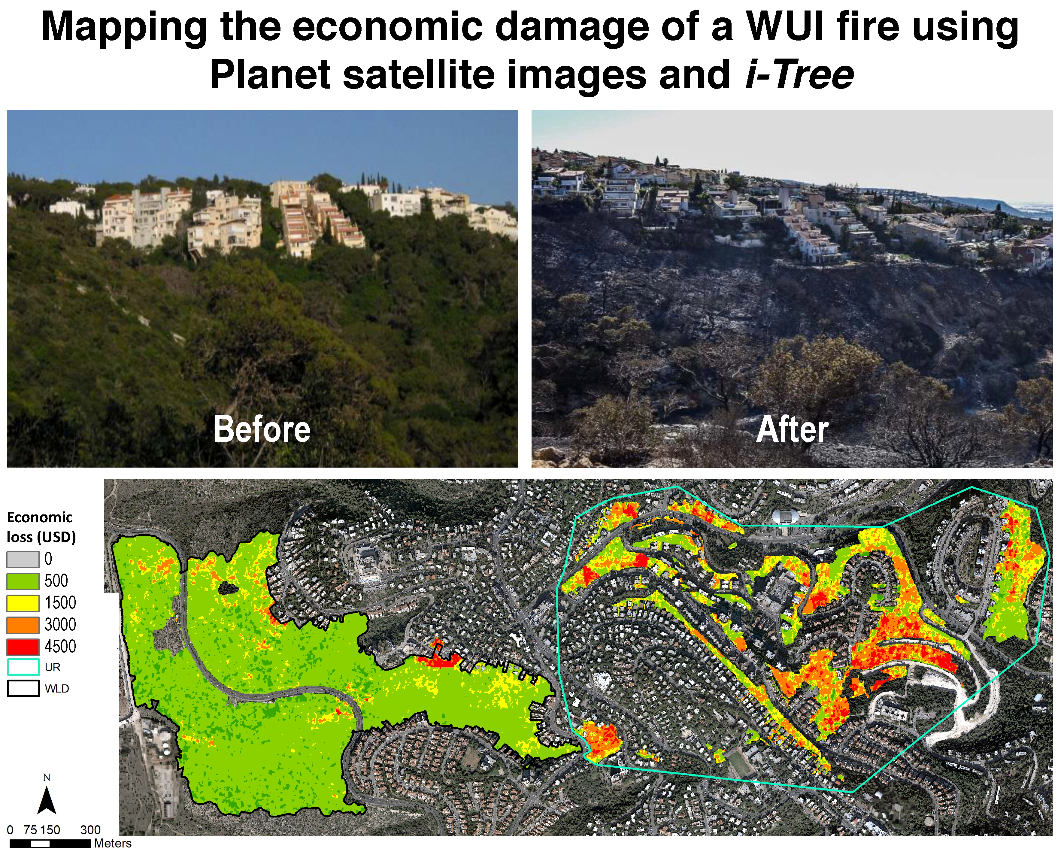
2.1. Study Area

The WUI study area is in the city of Haifa, which is located in the northern part of Israel (32°49′0″N, 34°59′0″E). The city of Haifa was built on the hillslopes of Mount Carmel, near the eastern coast of the Mediterranean Sea (Figure 1a). It is one of the largest cities in Israel (6.5 × 10³ ha), with a population of ca. 280,000 inhabitants [31]. In the WUI of Haifa, some large patches of the original native vegetation may be found, mostly Aleppo pines (Pinus halepensis Mill.) and common oak (Quercus calliprinos) trees. Some of these patches are located near residential buildings alongside ornamental species such as the Australian pine trees (Casuarina equisetifolia). The native vegetation of Mt. Carmel is currently preserved in the valley part of the city, as a part of the city’s urban plan [32].

The climate is a typical eastern-Mediterranean type, with dry, hot summers (June–August) and cool, rainy winters and autumns (October–May). The average annual rainfall varies with the elevation, from 550 mm∙yr⁻¹ to 750 mm∙yr⁻¹ at altitudes of 0 to 550 m above sea level, respectively [23].

2.2. The Fire of November 2016

At the end of November 2016, after several months without rain, and following strong easterly winds and extremely dry conditions, several fires were ignited in the central and northern parts of Israel [33]. One of these fires occurred within the city limits of Haifa. The fire lasted for two days (24–25 November 2016) before it was extinguished by firefighters [34]. The focus of the fire was at the grove area within the southwestern part of the city, advancing rapidly to the west towards the open area that surrounds the city (Figure 1b). The fire damaged residential areas in Haifa, as well as the ornamental and native vegetation in the WUI. A total of 164 buildings were burnt over a total area of ca. 121 ha [35].

3. Data and Methods

3.1. Satellite Images

Multi-temporal satellite imagery including 27 4-band PlanetScope images of high spatial resolution (3.125 m) were downloaded from Planet Labs (https://www.planet.com) for the period from 9 March 2016 to 19 October 2017. Images were downloaded in two formats: as PlanetScope images and as Ortho Scene Product images, both with four spectral bands in the blue, green, red, and near infrared spectrum (

Table 1. Wavelength range of Planet and Sentinel-2A satellites sensors for blue, green, red, and NIR spectral bands.

Band	Planet Scope 3-m (nm)	Sentinel-2A 10-m (nm)
Blue	455–515	448–546
Green	500–590	537–583
Red	590–670	545–583
NIR	780–860	763–909

).

In addition, 29 images of the Sentinel-2A (Sentinel-2MSI L1C) product were download from Sentinel’s Scientific Datahub (https://scihub.copernicus.eu/). Sentinel-2A images have also four spectral bands in the blue, green, red, and near infrared for the 10-m product (Table 1).

All images went through radiometric and sensor corrections and were orthorectified to a cartographic projection. Sentinel-2A images were atmospherically corrected using the Sen2Cor algorithm [36]. Vegetation indices were calculated from the spectral bands for Planet and Sentinel-2A (Section 3.2).

3.2. Vegetation Indices

Three satellite-based vegetation indices (VIs) were used to derive post-fire burn severity maps and pre-fire stand density and woody biomass maps for the study area at 3-m (Planet) and 10-m (Sentinel-2A) spatial resolutions. The three VIs are commonly used as proxies of green biomass and vegetation cover are the following:

3.2.1. NDVI

NDVI is the most widely used vegetation index [37]. It is based on the solar reflectance in the red (Red, 0.6 μm) and near infrared (NIR, 0.8 μm) wavelength bands (

Table 2. Formulation of satellite-based vegetation indices used in this study.

Index	Formulation	Reference
NDVI 1	$\mathrm{NDVI}=\frac{{\rho (\mathsf{\lambda }}_{\mathrm{NIR}}{)-\rho (\mathsf{\lambda }}_{\mathrm{Red}})}{{\rho (\mathsf{\lambda }}_{\mathrm{NIR}}{)+\rho (\mathsf{\lambda }}_{\mathrm{Red}})}$	[48]
GNDVI 2	$\mathrm{GNDVI}=\frac{{\rho (\mathsf{\lambda }}_{\mathrm{NIR}}{)-\rho (\mathsf{\lambda }}_{\mathrm{Green}})}{\rho \left({\mathsf{\lambda }}_{\mathrm{NIR}}\right){+\rho (\mathsf{\lambda }}_{\mathrm{Green}})}$	[49]
GCC 3	$\mathrm{GCC}=\frac{{\rho (\mathsf{\lambda }}_{\mathrm{Green}})}{\rho \left({\mathsf{\lambda }}_{\mathrm{Green}}\right)+\rho \left({\mathsf{\lambda }}_{\mathrm{Blue}}\right){+\rho (\mathsf{\lambda }}_{\mathrm{Red}})}$	[50]

¹ NDVI is the normalized difference vegetation index; ² GNDVI is the green NDVI; ³ GCC is the green chromatic coordinate index.

). As its name indicates, the NDVI is a normalized index with values in the range of −1 and 1, with full vegetation cover approaching the value of 1 and bare soil with values close to 0. Negative values usually indicate presence of water. The NDVI has some saturation problems over dense vegetation cover [38]. However, it was shown to be very reliable in monitoring vegetation dynamics in Mediterranean forests and woodlands, particularly for Mt Carmel, Israel [23]. It was also successfully used to assess burn severity in Mt Carmel forests and woodlands following the great fire of 2010 [23].

3.2.2. GNDVI

The GNDVI is very similar to the NDVI, with the difference that GNDVI uses the green band (Green, 0.5 μm) instead of the red (Table 2). It is believed to be more sensitive to chlorophyll—a concentration as compared to NDVI [39]—and thus, may be more accurate than NDVI over areas with dense vegetation cover. The GNDVI was also shown to be better correlated to burn severity than NDVI in several Mediterranean sites [40].

3.2.3. GCC

The green chromatic coordinate (GCC) index is based on the visible spectral wavebands using red, green, and blue bands with no information from the infrared band. The GCC is calculated as the ratio of green to the sum of the three bands (Table 2). It is correlated with the amount of green vegetation tissue, and is widely used in proximal sensing such as in-field PhenoCams [41,42] and digital camera [43,44]. The GCC is also used in vegetation monitoring from unmanned aerial vehicles (UAV) because of the relatively low cost RGB sensors mounted on UAVs [45,46,47].

The use of the GCC also expands the possibility of using images from Planet Doves prior to January 2016 when they acquired images only in the RGB spectral bands (since early 2015).

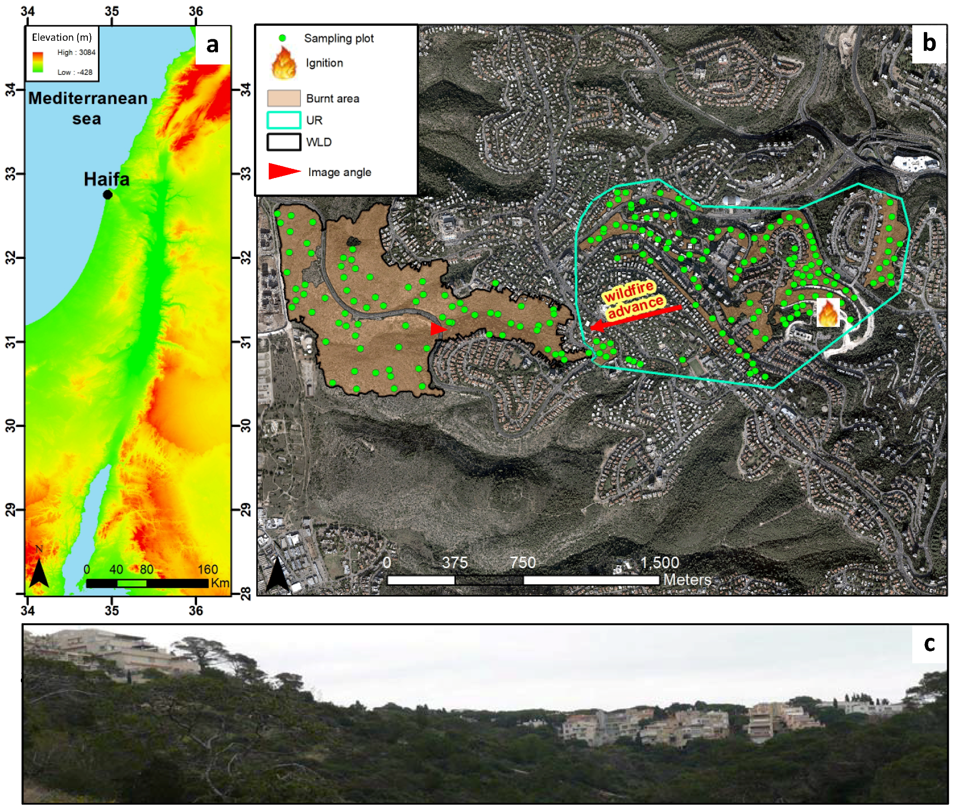
3.3. Using MODIS NDVI Time Series to Track Vegetation Phenology

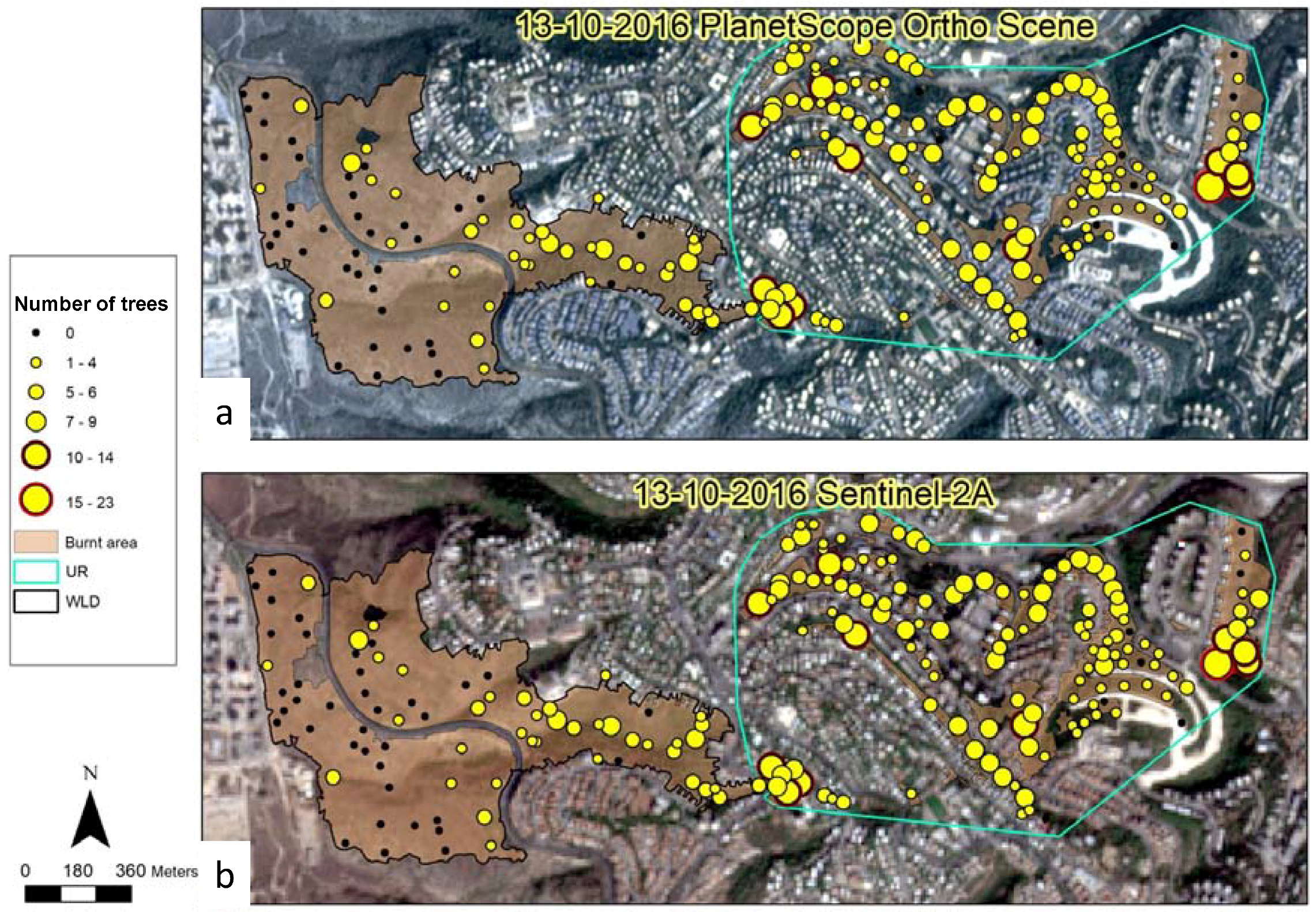
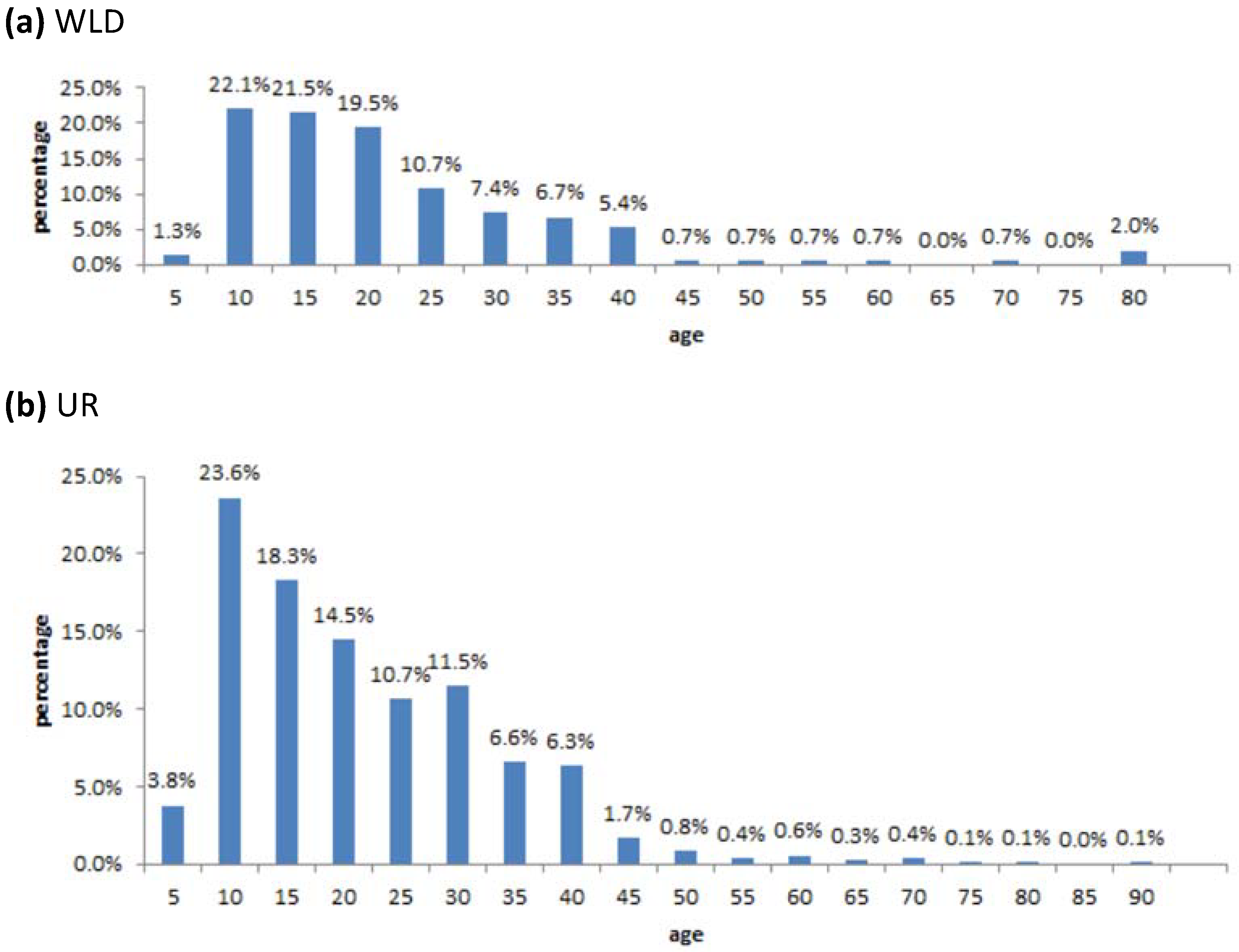
Helman et al. 2015 [23] showed that MODIS NDVI time series may be used to distinguish between ephemeral herbaceous understory vegetation and evergreen woody vegetation in Mediterranean environments. Using time series of the MOD13Q1 product, they demonstrated that the baseline of the NDVI time series corresponds to the signal coming from the trees, while the seasonal component of the time series mostly corresponds to the ephemeral herbaceous vegetation in the understory of the forests [23,37].

We used the technique proposed by [23] to find the relevant dates in which the woody vegetation mostly contributed to the VI signal. For that purpose, the NDVI derived from the 3-m and 10-m images (Planet and Sentinel-2A, respectively) were aggregated to the MODIS-pixel size and compared to the longer NDVI time series from MODIS (MOD13Q1) in the study area (Figure 2). Comparison was done using the Google Earth Engine platform after adding a constant value of 0.16 to the NDVI time series from Planet, due to a known shift towards lower values from Planet satellites [30].

The MOD13Q1 product is based on a single day maximum value criteria and is considered to be of a high quality and very reliable for vegetation monitoring [38]. We used a robust, locally-weighted regression and smoothing scatterplots (lowess) technique, as in [51,52], to reduce noise and uncertainties originating from cloud contamination and sensor artefacts (see green line in Figure 2).

Figure 2 shows the seasonal growth cycle of the vegetation in the MODIS-NDVI time series. The minimum value at the beginning of the season corresponds to the signal coming from the trees (evergreen woody vegetation), while the seasonal signal of NDVI corresponds mainly to the ephemeral herbaceous vegetation growth and senescence. The fire of November 2016 is evident in the NDVI time series as a sharp decrease clearly seen from the NDVI time series derived from the three satellites (Figure 2).

We used Figure 2 to select four dates that better represented the signal from the woody vegetation prior to the fire of November 2016 (

Table 3. Dates of images used prior to and following the fire of 24–25 November 2016.

Satellite	Before				After
	Date 1	Date 2	Date 3	Date 4	Date 5
Sentinel-2A	13 September 2016	13 October 2016	12 November 2016	22 November 2016	11 January 2017
Planet	23 August 2016	13 October 2016	12 November 2016	21 November 2016	5 December 2016

). This, in order to avoid mixed-pixel signal from the herbaceous vegetation and soil background [53]. VIs calculated from the four images (dates) were used to derive stand density and woody biomass maps through calibration with plot-based stand density and tree diameter at breast height (DBH) measurements (Section 3.4). The image with the VI that best correlated with the aforementioned biophysical parameters was chosen to derive stand density and woody biomass maps. It was also used with the first available image following the fire to derive burn severity map. In the case of Sentinel-2A, this was ca. a month and a half after the fire, while first Planet image was available 11 days after the fire (Table 3).

3.4. Field Survey

We divided the study area into two domains: (i) urban (UR) and (ii) wildland (WLD) (Figure 1b). The two domains differed in terms of total area (40 ha vs. 85.3 ha for UR and WLD, respectively), as well as in vegetation composition. The dominant tree species in WLD are mostly native species, like Aleppo pines (Pinus halepensis Mill.) and common oaks (Quercus calliprinos Webb), while the UR domain contains a greater variety of ornamental species and a much lower percentage of native species (

Table A1. Tree species distribution in urban (UR; top) and wildland (WLD; bottom) domains.

Tree Species	Trees per Plot	From Total (%)	DBH (cm)	Density (103 trees ha−1)
Acer obtusifolium Sm.	2	0.30	10.0	14.9
Ailanthus altissima (Mill.) Swingle	15	2.3	15.3	111.2
Albizia lebbeck (L.) Benth	2	0.3	17.5	14.9
Arbutus andrachne L.	4	5.6	10.0	37.1
Casuarina equisetifolia L.	34	5.1	28.1	251.9
Ceratonia siliqua L.	1	0.2	26.0	7.5
Cercis siliquastrum L.	5	0.8	19.4	37.1
Crataegus azarolus L.	4	0.6	12.8	29.0
Cupressus sempervirens L.	108	16.3	19.4	800.0
Dalbergia sissoo Roxb.	2	0.3	32.5	14.8
Eucalyptus camaldulensis Dehn.	34	5.1	36.7	251.9
Euphorbia tirucalli L.	2	0.3	19.5	14.9
Laurus nobilis L.	15	2.3	10.6	112.0
Melia azedarach L.	5	0.8	15.2	37.0
Olea europaea L.	4	0.6	13.5	29.7
Phoenix dactylifera L.	1	0.2		7.5
Pinus brutia Ten.	31	4.2	26.7	229.7
Pinus halepensis Mill.	172	25.9	27.4	127.4
Pinus pinea L.	6	0.9	28.3	44.5
Pistacia palaestina Boiss.	28	25.9	9.7	207.5
Quercus calliprinos Webb.	138	20.8	12.7	1022.3
Rhamnus alaternus L.	36	5.4	7.8	266.7
Rhamnus lycioides L.	3	0.5	9.0	22.9
Ulmus minor Mill.	5	0.8	13.4	37.0
Washingtonia robusta H.Wendl	2	0.3	32.5	14.9
Ailanthus altissima (Mill.) Swingle	7	3.1	12.4	91.0
Casuarina equisetifolia L.	4	1.8	53.8	52.0
Ceratonia siliqua L.	10	4.4	24.4	12.9
Cupressus sempervirens L.	4	1.8	19.5	52.0
Laurus nobilis L.	10	4.4	20.3	12.9
Olea europaea L.	2	0.9	15.0	26.0
Pinus canariensis C. Smith	1	0.4	35.0	13.0
Pinus halepensis Mill.	87	38.5	23.1	1129.9
Pinus pinea L.	48	21.2	24.4	623.4
Pistacia palaestina Boiss.	1	0.4	32.0	13.0
Quercus calliprinos Webb.	51	22.6	14.4	624.2
Rhamnus alaternus L.	1	0.4	12.0	13.0

Trees per plot refers to the number of trees in each 100 m² plot; Percentage from total is % of trees from total number of trees in all plots; DBH is the mean stem diameter at breast height in cm; Density is the tree stand density in 10³ trees per ha.

).

A field-based burn severity map with polygons containing three levels (low, moderate, and high) was created using orthophoto (taken in December 2016) and complementary information from an extensive field survey [35]. Burn severity was characterized in the field following conventional classification [54,55]. It was found that nearly 64% of the inspected area was within the low-moderate burn severity class, while 36% was in the high severity class. A second field survey was conducted approximately one month after the fire, based on the orthophoto-based burn severity map. Tree diameter at breast height (DBH in cm tree⁻¹) was measured for trees in 212 randomly selected 10 m × 10 m plots within the burnt area (Figure 3). Trees within each plot were characterized by species type and counted to derive stand density (trees ha⁻¹) in the plot (Figure 3 and Table A1).

Tree stand density was found to be significantly higher (p < 0.001; Student’s t-test) in plots within the UR domain (5.4 trees plot⁻¹; N = 135) than in the WLD domain (2.2 trees plot⁻¹; N = 77). In general, the WLD was much shrubbier than the UR domain.

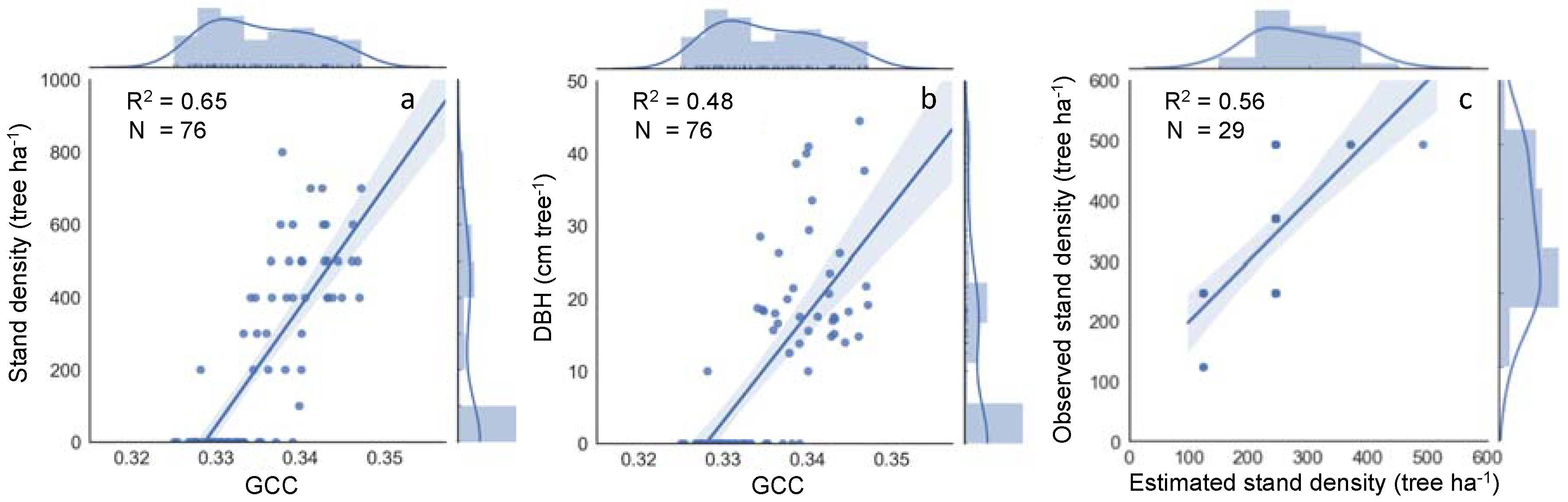
3.5. Deriving Tree Density and DBH Maps from Calibrated Satellite Data

The three VIs calculated from each of the four images prior to the fire (Table 3), were regressed against tree density and mean DBH from field survey to obtain an empirical relationship between the two. Because of the mismatch between the spatial resolutions of the satellite and field data, VIs were averaged over a window of 3 × 3 (3 m) pixels. The image that provided the best coefficient of determination (i.e., highest R²) was used to calibrate the three VIs and derive stand density (trees ha⁻¹) and DBH (cm tree⁻¹) maps for the WUI area.

Six tree density maps and six DBH maps (i.e., from 3 VIs × 2 satellites) were created using the best empirical relationships. These maps were then used to derive maps of aboveground woody biomass (AGB) loss (Section 3.6) and environmental economic loss (Section 3.9).

3.6. Deriving Aboveground Woody Biomass from Vegetation Indices

We used the DBH maps to produce new AGB maps following a general allometric equation [56]:

$${\mathrm{AGB}=\mathrm{e}}^{\mathsf{\alpha }+\mathsf{\beta }·\ln \left(\mathrm{DBH}\right)}$$

(1)

where $\mathsf{\alpha }$ and $\mathsf{\beta }$ are the intercept and slope of the linear regression found by Jucker et al. (2017) [56] for ln(AGB) and ln(DBH) relationships in a global synthesis of 108,753 trees. DBH in Equation (1) is in cm per tree and the AGB is retrieved in kg tree⁻¹. The AGB per tree was multiplied by the stand density to derive AGB in kg ha⁻¹. The AGB map was used with the burn severity map to assess woody biomass loss caused by the fire (Section 3.8).

3.7. Burn Severity Classification Using Vegetation Indices

Burn severity was calculated from the three VIs as the difference between the VI value prior to and following the fire ($\Delta$VI = VI_before − VI_after) [23]. A larger (positive) $\Delta$VI would correspond to a higher level of burn severity and vice versa. The image that best represented the woody vegetation status before the fire was chosen as VI_before, instead of taking the image with the closest date prior to the fire (Figure 2). We then compared the field-based burn severity level map (from Section 3.4) with the $\Delta$VI map using Two-way ANOVA with Tukey HSD separation procedure to test for significant differences between averaged $\Delta$VI in the areas classified in the field as low, moderate, and severe classes.

3.8. Assessing Burned Trees and Woody Biomass Loss in the Fire Area

The number of trees that were consumed by the fire (or which died following the fire) were calculated from the satellite-derived stand density and burn severity maps. Following in-field observations and observations reported by Meigs et al. 2009 [57], we applied assigned values of 22%, 54%, and 98% burned trees to areas that experienced low, moderate, and high burn severity, respectively. Average values of 10%, 25%, and 40% were applied on the AGB map to derive the woody biomass consumed by the fire in low, moderate, and high severity burned areas, respectively [57]. Higher values were reported in Mediterranean environments of 25%, 47%, and 65% [58], and 32%, 52%, and 85% [59] for low, moderate, and high burn severities. These values are generally within the range provided by Meigs et al. 2009 [57]. Nevertheless, we decided to use here the aforementioned averaged values provided by Meigs et al. 2009 [57], which give a more moderate and realistic estimation compared to the qualitative assessment which was undertaken during the field survey in our study area.

3.9. Use of Economic Model to Evaluate Fire Damage in WUI

We adopted the i-Tree method to assess the economic damage caused by the fire in the WUI of Haifa [60]. In i-Tree, the annual contribution of each tree to the urban environment is assessed in economic terms. The i-Tree method was adopted by several countries, including Israel, Australia, and the UK. In i-Tree, the annual economic value of each tree is based on the following formula:

TotVal (USD) = Base value × DBH × f_SpecVal × f_LocVal × f_CanopCondVal

(2)

where TotVal is the total value of the tree in US dollar (USD) per year; DBH is the diameter of the tree at breast height (in cm); f_SpecVal is the tree species value factor (f_SpecVal ranges between 0 and 1), usually provided by tree experts; f_LocVal is the location value factor with values between 0 and 1. It is based on the extent of exposure that people have to the various benefits of the tree (e.g., a tree located within the city area gains higher f_LocVal value than a tree located at the interface between the city’s buildings and wildland area); f_CanopCondVal is a canopy condition value factor, which also ranges between 0 and 1 depending on the tree’s canopy condition (for e.g., a trimmed canopy gets a lower f_CanopCondVal value than a fully developed untrimmed canopy). In this study, we used the following f_CanopCondVal classification of the Israel Ministry of Agriculture and Rural Development (MOAG): a tree with a highly-trimmed canopy was assigned a value of 0.6, tree with a moderately trimmed canopy was given a value of 0.85, and for a tree with a fully developed, untrimmed canopy a f_CanopCondVal value of 1.0 was used. A base value of 2.5 USD per cm (i.e., DBH) is used as a maximum potential value in Equation (2).

Finally, since we needed the total value of the tree over its entire lifecycle, the annual tree value calculated using the i-Tree approach was multiplied by the average life cycle of the tree species after reducing its pre-fire age (see Figure A1 for tree age distribution in the burnt area). Future benefits were reduced using a 3% discount rate, which refers to the discount in future welfare. This discount rate is common in the literature [61], and is currently adopted by the Israeli The Ministry of Environmental Protection. The following vector layers were created to calculate the spatially distributed economic damage using the i-Tree method:

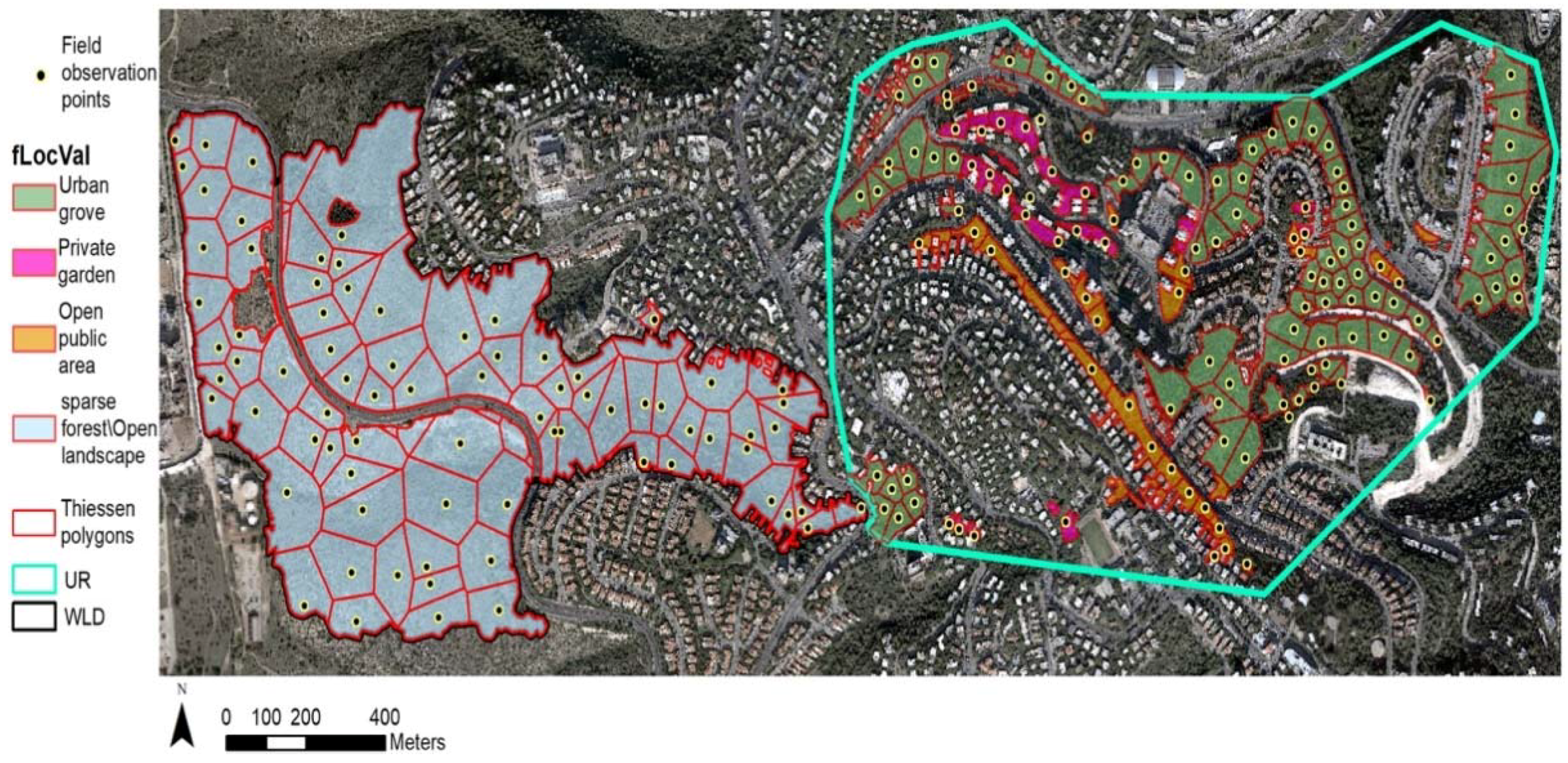
• The Thiessen polygons method [62] was applied to derive tree species distribution within the burnt area by using the tree species distribution assessed at the 212 field plots. Then, a f_SpecVal layer was derived for the entire burnt area at the Thiessen polygons resolution.
• The f_LocVal layer was produced by determining specific f_LocVal value for each Thiessen polygon through the use of a zoning map of Haifa (http://gis.haifa.muni.il/haifa_html5/) and a pre-fire aerial photograph taken in 2016 (Figure A2). Whenever uncertainty regarding the proper f_LocVal value occurred, we consulted Mr. Israel Galon, the director of the Department of Flowers and Plant Engineering in MOAG, previously the director of the forestry services in MOAG; Mr. Galon led the adaptation of i-Tree to the Israeli forest system.
• Canopy condition were determined for each tree per plot using a pre-fire very-high-spatial resolution aerial photograph. This was then used to assign the f_CanopCondVal for each Thiessen polygon, as described above.

The aforementioned layers were used in conjunction with the satellite-derived DBH and burned trees raster maps to derive a spatially continuous economic loss map at a spatial resolution of 3m.

3.10. Accuracy Assessment and Estimated Uncertainty

We conducted an accuracy assessment of the main maps derived from our methodology: (1) the stand density map, and (2) the burn severity map. Validation for the stand density calibration equation (Section 3.5) was made using a field-based stand count conducted during a field survey by a private company of environmental planning (Miller-Blum & Co. Environmental Planning Ltd.) in 2016 in an area nearby the WUI study area (2 km apart). A map of 29 plots of 10 × 10 m with a number of trees and their relative location within the plot area was provided by Miller-Blum & Co. Environmental Planning Ltd. This map was then used to compare with the stand density derived from Planet GCC image and the calibration equation. Validation was conducted by collocating 3 × 3 Planet pixels within the plot area while averaging the stand density over the 3 × 3 pixels. The coefficient of determination (R²) was used as an accuracy metric for this validation.

The burn severity classification map derived from satellite data (Section 3.7) was validated with a vector map created from a very-high-spatial resolution aerial photograph (7.5 cm) taken in 28 November 2016 and the information derived in the field, as in [23], using a confusion matrix technique. The overall accuracy (OA) and the kappa of the confusion matrix were used as accuracy metrics for the satellite-derived burn severity map.

We used the mean absolute error (MAE) of the regressions obtained from Section 3.5 and the different ranges in percentages of consumed woody biomass per burn-severity class given in Section 3.8 to provide the uncertainty estimations of the consumed woody biomass, the stand density, and the economic loss through maps of low-to-high estimates of these variables (Results presented in Figure A3, Figure A4, Figure A5 in the Appendix).

4. Results

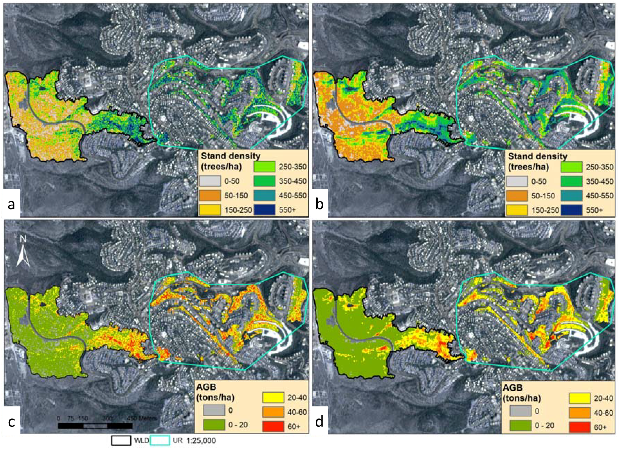
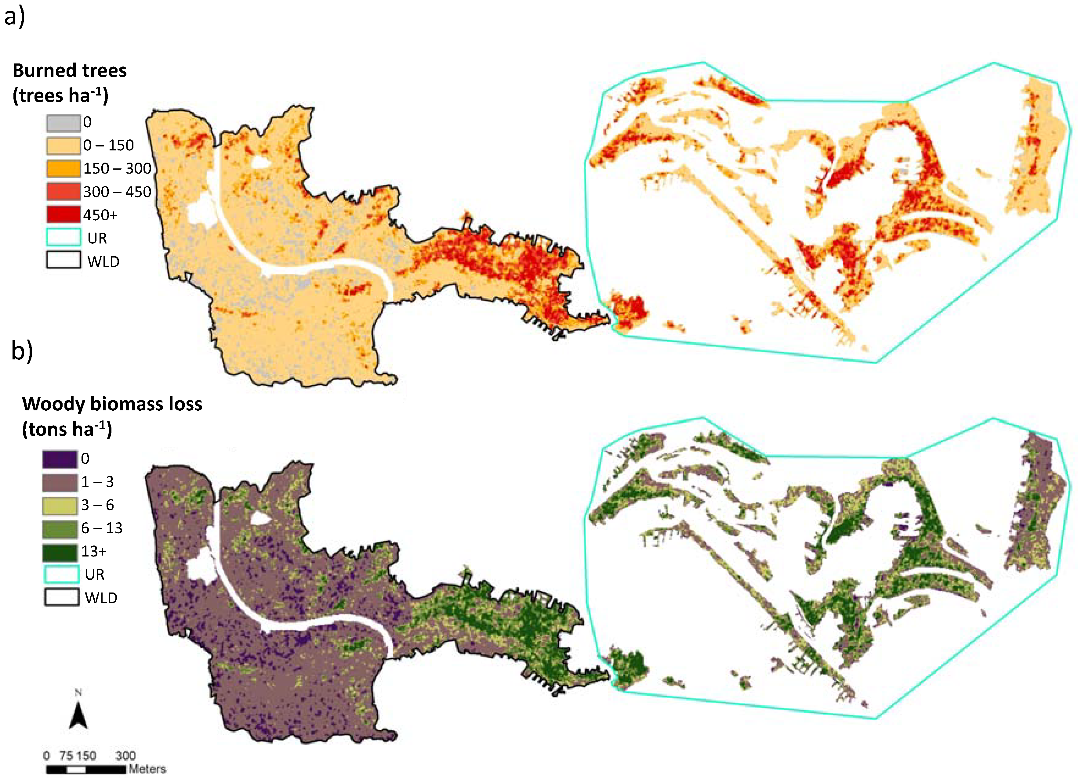
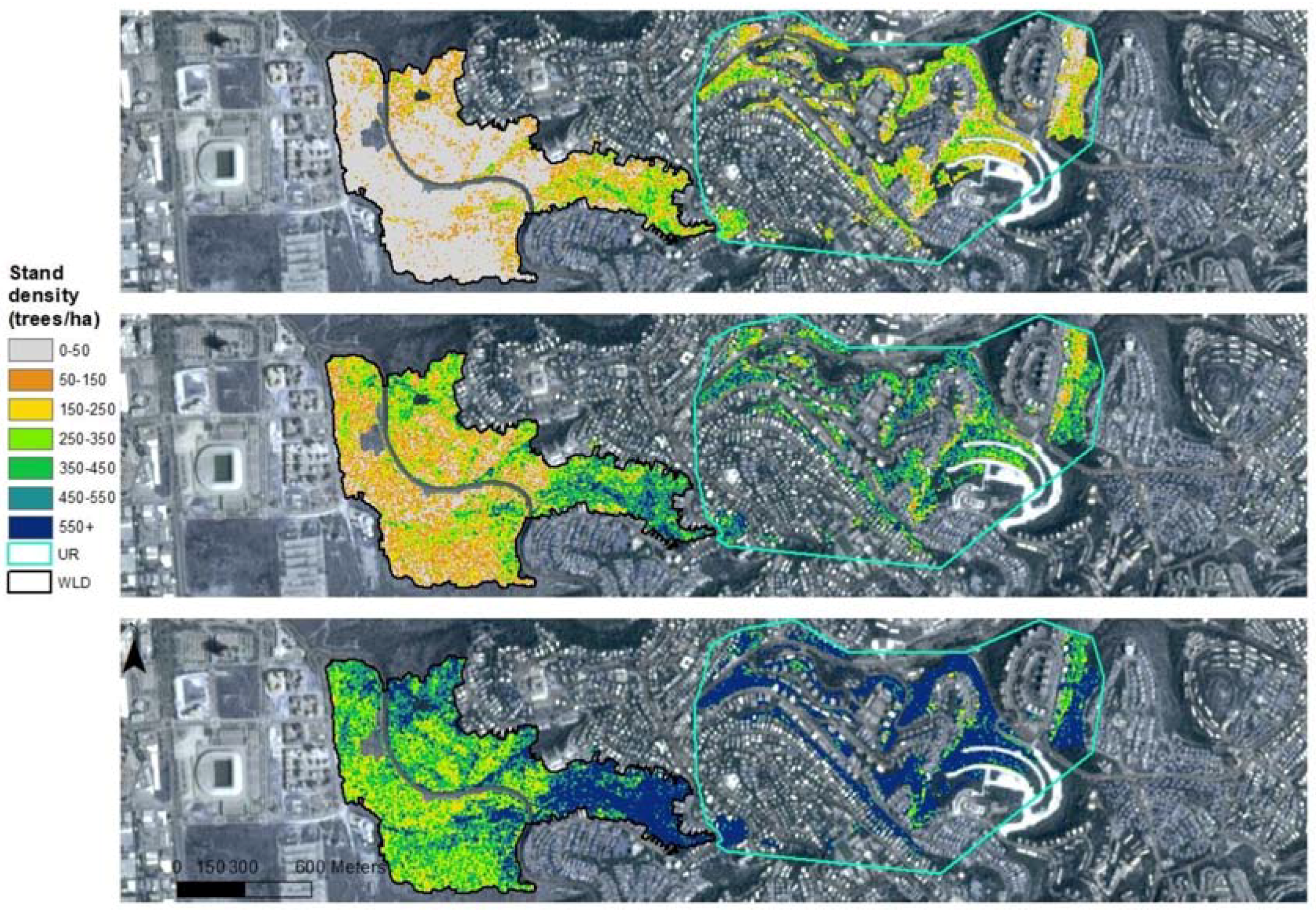
4.1. Stand Tree Density and Woody Biomass in Haifa’s Wildland-Urban Interface Area

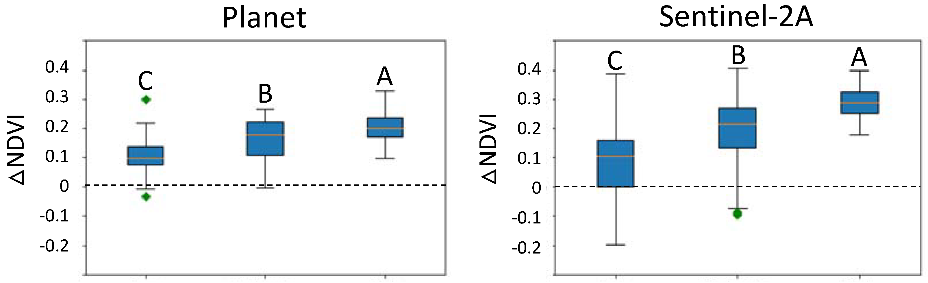
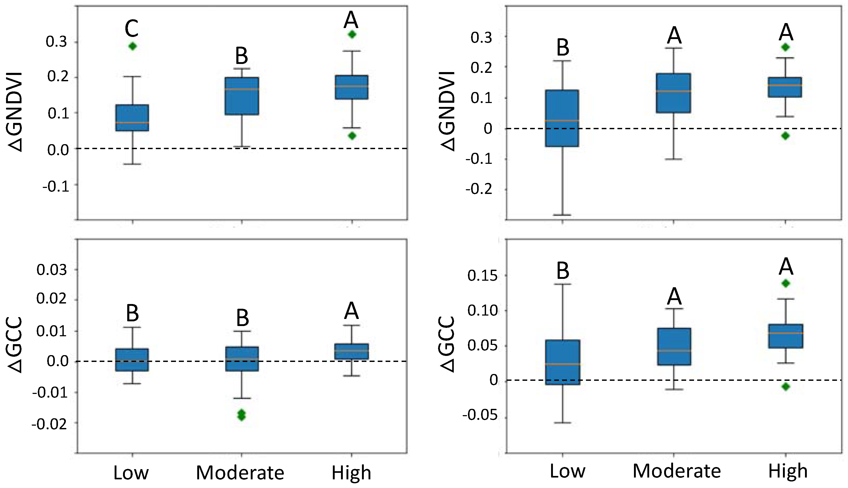
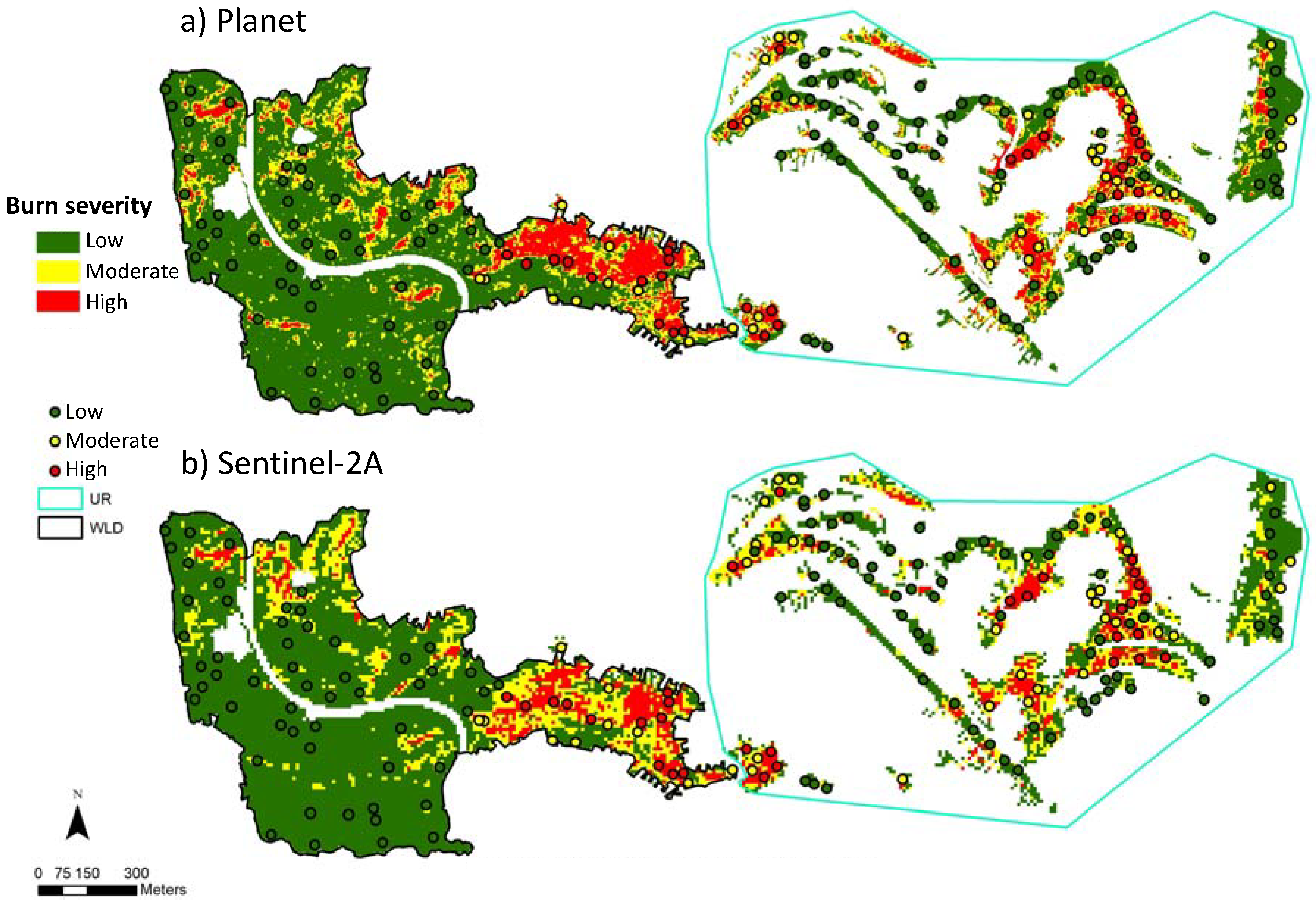
All three vegetation indices showed positive moderate relationships with field-based stand density measurements (

Table 4. R² of the correlation between the three VIs (NDVI, GNDVI and GCC; see Table 2) and stand density and DBH measured at the field survey. VIs were correlated with stand density and DBH using four images taken at different dates prior to fire. Best correlations are indicated in bold.

	Planet			Sentinel-2A
Date	NDVI	GNDVI	GCC	NDVI	GNDVI	GCC
Tree density
22 November 2016	0.45	0.26	0.49	0.54	0.41	0.62
12 November 2016	0.27	0.27	0.45	0.55	0.42	0.64
13 October 2016	0.47	0.50	0.56	0.51	0.47	0.56
23 August 2016	0.54	0.55	0.65	0.58	0.50	0.59
AVG	0.43	0.40	0.53	0.54	0.45	0.60
DBH
22 November 2016	0.23	0.24	0.30	0.29	0.22	0.29
12 November 2016	0.27	0.27	0.36	0.31	0.25	0.37
13 October 2016	0.22	0.29	0.35	0.35	0.37	0.31
23 August 2016	0.37	0.39	0.48	0.31	0.27	0.32
AVG	0.28	0.30	0.37	0.31	0.28	0.33

). R² of the VIs-stand density correlations ranged between 0.26 and 0.62, where the highest correlation found was with the GCC for both satellites and with the image corresponding to 23 August 2016 for Planet and 12 November 2016 for Sentinel-2A. The R² of the VIs-DBH correlations were lower, i.e., within the range of 0.22 and 0.48, with GCC being the best VI for Planet and GNDVI and GCC for Sentinel-2A (Table 4).

Figure 4 shows a scatterplot of GCC vs field measurements of stand density and DBH for Planet (image acquired in 23 August 2016). The GCC calibrated stand density linear regression equation was successfully validated with the stand count conducted in an area nearby the WUI, with R² = 0.56 (Figure 4c).

We then used the GCC calibrated stand density and DBH equations to derive the satellite-based stand density and DBH maps.

Figure 5 shows the stand density and AGB maps from Planet and Sentinel 2-A for UR and WLD domains. Planet-derived stand density uncertainty maps using the MAE of the linear fit are provided in Figure A3. Stand density and AGB were notably higher at the eastern parts of the WLD domain, near the urban area, and at the grove area within the UR. In general, Planet-derived maps show slightly higher stand densities/AGBs at the grove area within the UR domain.

The mean stand density and AGB, which were notably higher in the UR than in the WLD, are shown in

Table 5. Tree stand density (trees ha⁻¹) and AGB (ton ha⁻¹) in the UR, WLD and total burnt area (UR + WLD).

Domain	Stand Density (trees ha−1)		AGB (ton ha−1)
	Mean	std	Mean	std
UR	414.85	160.69	20.43	27.64
WLD	222.42	165.27	5.30	13.47
WLD + UR	318.63	162.98	10.21	20.48

.

4.2. Burn Severity

Next, burn severity classification was derived from the different VIs. Figure 6 shows a boxplot of the $\Delta$VI values for the three burn severity classes determined in field. In general, $\Delta$NDVI was better correlated with burn severity, followed by $\Delta$GNDVI. For both indices, there was a significant difference between $\Delta$VI values of the different burn severity classes (p < 0.05 using ANOVA followed by Tukey HSD). There was no significant difference, though, between $\Delta$GCC values in low, medium, and high burn severity areas.

Hence, we used $\Delta$NDVI to derive a continuous burn severity map at the spatial resolution of the satellite images, providing low, medium, and high severity classification at the high spatial resolution of the satellite images (Figure 7). The classification provided in Figure 7 was further validated with the vector layer derived from a combined very-high-spatial resolution aerial photograph and in-field assessment.

Table 6. Confusion matrix for the three burn severity classes (all values are presented as percentages from total). In bold is the percent (%) hit for each burn class category.

	Reference Data
Classifier Results	Low	Moderate	High	Producer Accuracy (Precision)
Low	93.7	6.3	0.0	93.7
Moderate	20.1	70.5	9.4	70.5
High	0.0	20.4	79.5	79.5
User Accuracy (Recall)	93.8	66.3	86.2

summarizes the results of this validation. The overall accuracy (OA) of the satellite-derived burn severity map was 87%, with a kappa of 0.75.

Figure 7 shows the spatial burn severity distribution at the UR and WLD domains with severely burned areas, particularly at the high stand density and AGB woodland areas of the city (see Figure 5). In the UR, 52% (52%) of the area was classified with low severity, while 26% (23%) and 22% (25%) were classified as medium and high burn severity, respectively, from the Planet (Sentinel-2A) $\Delta$NDVI map. In the WLD, where the stand density and AGB were substantially lower, 71% (73%) of the area was classified with low severity, while only 17% (20%) and 12% (7%) were classified as medium and high burn severity classes from Planet (Sentinel-2A) $\Delta$NDVI.

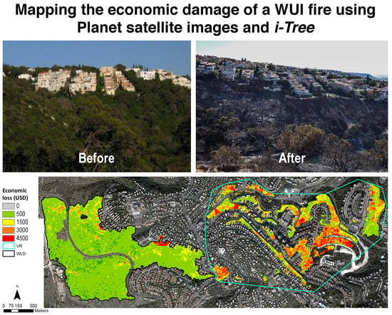
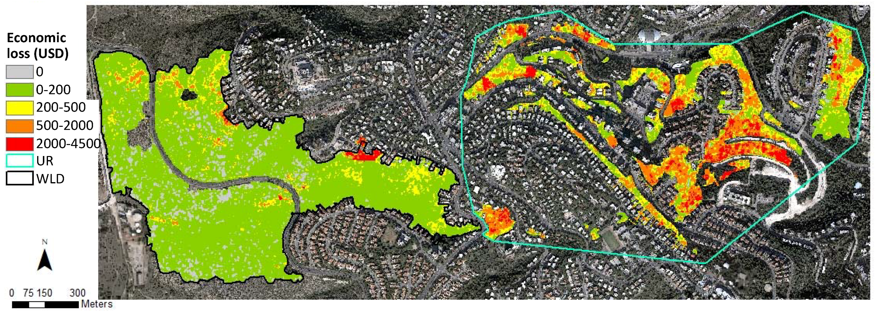
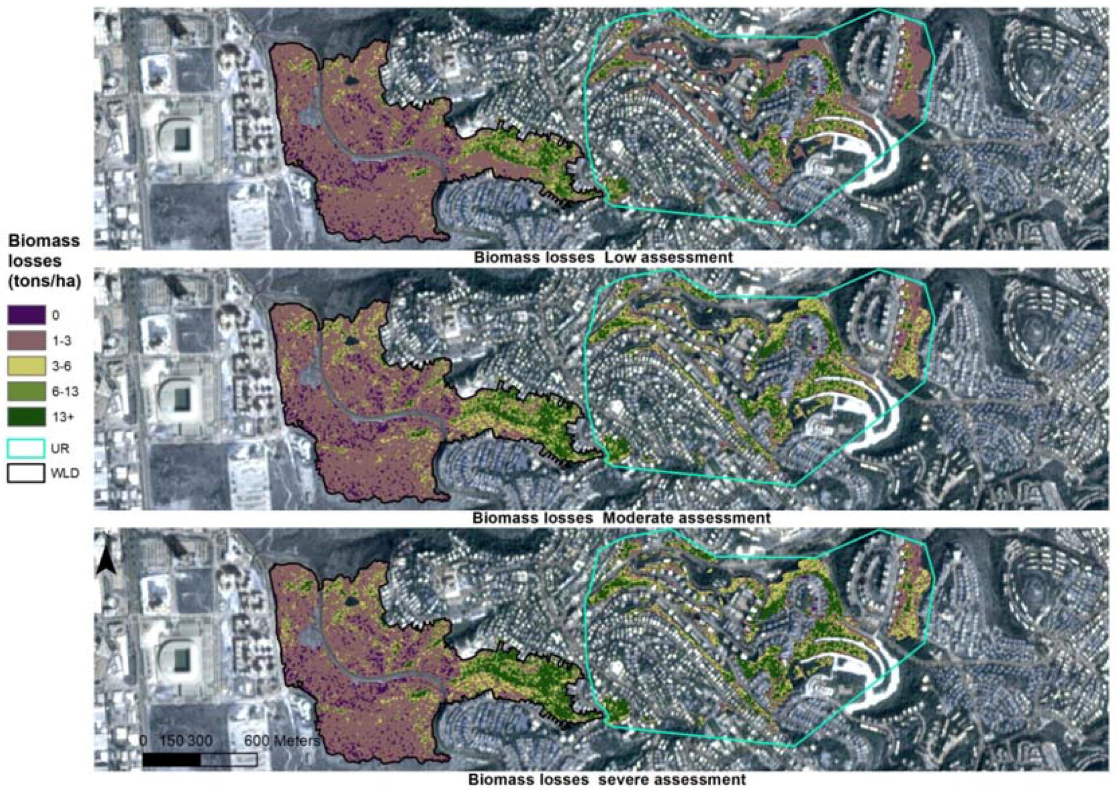
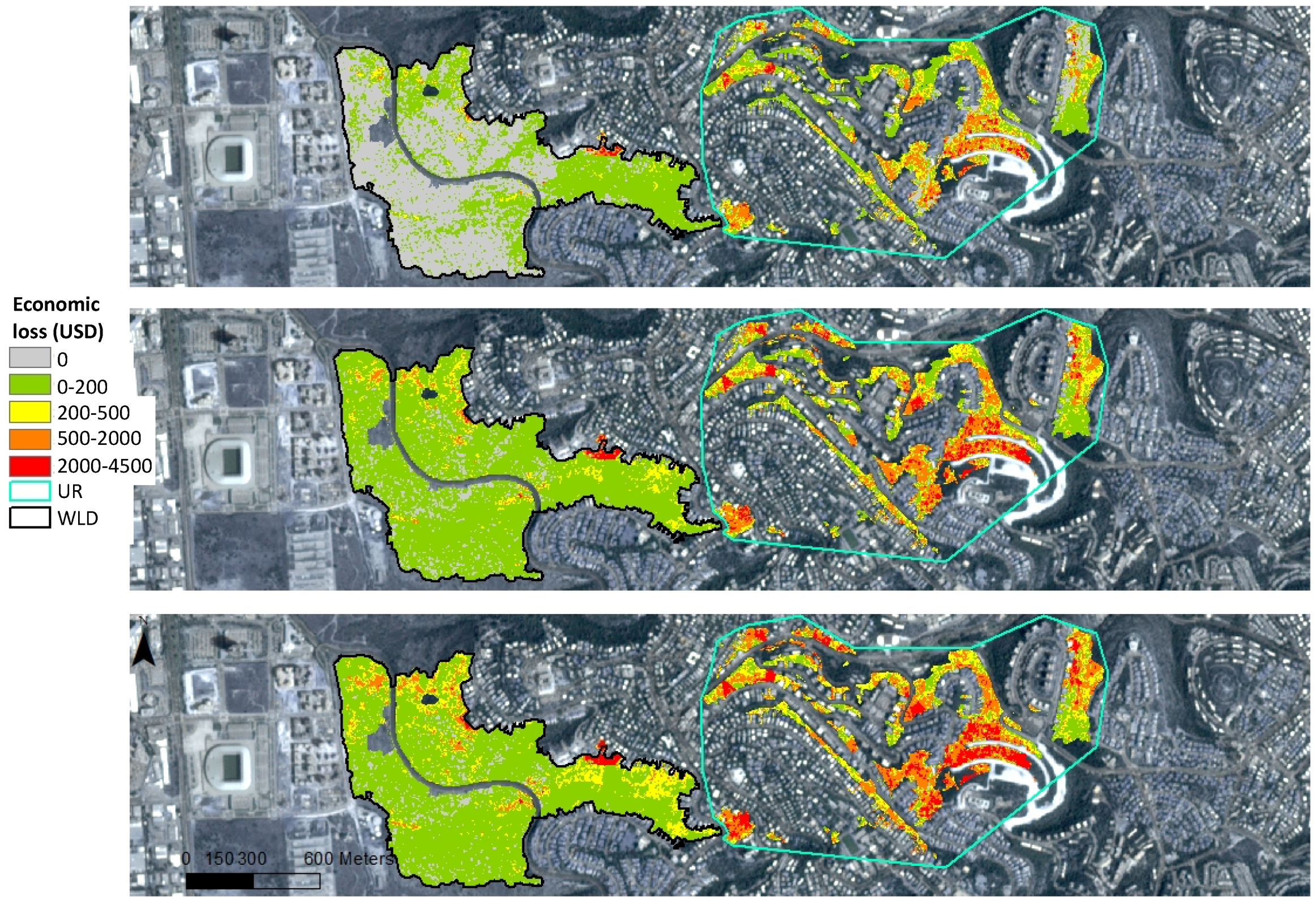
4.3. Environmental and Economic Damages of the Fire

Finally, burned trees and woody biomass loss maps were created from the burn severity, stand density, and DBH maps (Figure 8). As expected from the stand density map (Figure 5 and Table 5), the mean woody biomass loss was greater in the UR domain than in the WLD domain (6.89 ton ha⁻¹ compared to 2.81 ton ha⁻¹). The total number of burned trees was comparable in both domains, with 8120 vs. 8700 burned trees in UR and WLD, respectively (203 and 102 trees ha⁻¹, respectively). Results reflecting estimated uncertainty of stand density and consumed biomass are provided as maps of low and high estimates in Figure A3 and Figure A4.

The spatially distribution economic loss caused by the fire of 2016 in Haifa, and calculated with the i-Tree model, is shown in Figure 9, while lower and higher estimates from the uncertainty analysis are shown in Figure A5.

Figure 9 shows that the greater economic loss is in UR. This is in spite of the large quantity of burned trees in the eastern part of the WLD domain (Figure 8a), and an equal amount of burned trees in the area of the two domains. The damage in the UR was estimated at 840 ± 210 K USD per hectare, with a total loss of 33,600 ± 8400 K USD for the entire UR burnt area, while in WLD it was one order of magnitude smaller, estimated at 85.6 ± 21.4 K USD per hectare, with a total damage of more than 7300 ± 1800 K USD for the entire WLD burnt area. The total economic damage related to environmental damage, of the fire of 2016 in the WUI of Haifa was estimated at ca. 41 ± 10 M USD.

5. Discussion

Results of burn severity from Planet VIs were spatially compatible with ground survey burn severity classifications in both the WLD and UR domains. This demonstrates the potential use of high-spatial-resolution Planet images for burn severity assessment in the WUI. Previous studies using high and medium spatial resolution satellite images showed successful assessment of burn severity in WLD [23,25,63]. However, as far as the authors are aware, this study is the first to provide a burn severity assessment at the WUI.

Planet Doves provide a limited number of four spectral bands, lacking the shortwave infrared (SWIR) band. The SWIR is the most frequently-used band for burn severity mapping, successfully tracking burn severity variability across the burnt area [13,64]. Previous studies have shown that SWIR-based indices are usually preferable over NIR-based VIs [25], and in some cases, even essential when used for burn severity monitoring in Mediterranean ecosystems [19]. However, in this study, we found that simple NIR-based VIs, like GNDVI and NDVI, may provide satisfactory results in terms of burn severity assessment.

We found that, in general, the NIR-based VIs (i.e., GNDVI and NDVI) performed better in terms of burn severity assessment than the RGB-based GCC index. This may be because of the higher sensitivity that GNDVI and NDVI have to vegetation due to their use of the NIR band [65]. Another reason may be shadow effects, which usually increase with spatial resolution, particularly in RGB-based indices [66].

Comparisons with the more reliable Sentinel-2A satellite revealed that Planet may provide high-quality images for fire monitoring and tree parameter assessments in the WUI. Moreover, the advantage of the temporal resolution of Planet—which has been improved since 2016—over that of Sentinel-2A was essential for tracking vegetation status immediately after the fire. The first available image from Sentinel-2A was 48 days after the fire (Table 3) when herbaceous vegetation had already started to grow, thereby affecting the VI signal [29] (see also Figure 2). This was probably the reason for the wider area classified by Sentinel-2A as medium instead of high burn severity in the WLD (where herbaceous vegetation is widely present) compared to Planet (a ratio of 2.86 compared to 1.42 of medium/high percentage area in WLD, respectively; see also Figure 7). Differences between the two satellite sensors for the same date (Table 4) were likely due to differences in the width of the spectral wavelength bands (see Table 1), and to the different spatial resolution.

A recent study using Planet VIs showed that the high spatio-temporal resolution of Planet images may be used to track changes in stem water potential in Mediterranean vineyards [53]. This study also showed that simple Planet-derived vegetation indices can be used to derive important parameters of forest structure, such as stand tree density and DBH in a highly fragmented Mediterranean system composed of a variety of plant species (Table A1). The stand densities in our study area were within the range reported for similar Mediterranean systems [67]. Such results were also found in similar ecosystems in Greece [68] using Sentinel-2A images and with higher spatial resolution images acquired from the QuickBird satellite [69]. However, stand density was previously impossible to derive in urban areas with the coarser spatial resolution of Landsat (30 m) because of a mixed signal from features such as buildings, roads, and other impervious surfaces [70].

Finally, with regard to the economic evaluation of the fire damage to the urban forest in the WUI, our total estimated economic loss was of 41 ± 10 M USD based on i-Tree model, with some adaptations to the Israeli case. Notably, several methods were suggested to quantify value of trees in urbanized/near urbanized areas. These methods can be categorized into three approaches: the cost approach (e.g., Depreciated Replacement Cost, which assumes that the tree benefits can be reproduced by replacing the tree [71]), the market approach, which accounts for the trees’ wholesale values [72], and the benefit-based approach, which is based on future stream of benefits that a tree might produce. While a plethora of such benefits were acknowledged in the literature (see [73] for an exhaustive description), not all have actually been quantified. In turn, quantified benefits include energy conservation (e.g., due to shading effects and reductions in the urban heat island), surface and storm-water runoff reductions, atmospheric carbon dioxide reductions, and increased property values.

Finally, while some studies have found other substantial benefits such as lower levels of violence and stress in neighborhoods surrounded by trees, the i-Tree model currently lacks quantification of these benefits [60,74,75]. However, we found the i-Tree method to be the most appropriate considering our primary objectives, the locations of the trees, and the availability of data. Other benefit-based methods are based on variables that are more subjective, and thus, difficult to measure (e.g., historical significance). Nevertheless, as with many other methods, our method suffers from some limitations, specifically due to lack of accurate data (for example data on the exact condition of the trees). Future studies may improve the results obtained here by using more frequent high spatial resolution satellite schemes, providing more accurate information on trees’ species and condition. In addition, a sensitivity analysis using the i-Tree model may improve economic evaluation, accounting for uncertainty in economic loss estimates.

6. Conclusions

Results from this study demonstrate that images acquired from the high-spatial-resolution Planet Doves database may be used to derive tree parameters such as stand density and DBH using simple vegetation indices. It also shows that burn severity mapping may be conducted using Planet images in the complex WUI area. Using a simple economic model that evaluates the annual cost of a tree in conjunction with Planet derived tree-parameters and burn severity maps, we were able to estimate spatially distributed and total economic loss to the urban forest in the WUI of Haifa caused by the fire of 2016. This methodology may be applied elsewhere, enhancing pre- and post-fire monitoring in WUI areas, for a better allocation priority of economic resources and specific treatment actions directed towards minimizing economic losses due to potential future WUI fires.

References

1. Radeloff, V.C.; Helmers, D.P.; Kramer, H.A.; Mockrin, M.H.; Alexandre, P.M.; Bar-Massada, A.; Butsic, V.; Hawbaker, T.J.; Martinuzzi, S.; Syphard, A.D.; et al. Rapid growth of the US wildland-urban interface raises wildfire risk. Proc. Natl. Acad. Sci. USA 2018, 201718850. [Google Scholar] [CrossRef] [PubMed]
2. Mitsopoulos, I.; Mallinis, G.; Arianoutsou, M. Wildfire Risk Assessment in a Typical Mediterranean Wildland–Urban Interface of Greece. Environ. Manag. 2015, 55, 900–915. [Google Scholar] [CrossRef] [PubMed]
3. Tedim, F.; Xanthopoulos, G.; Leone, V. Chapter 5—Forest Fires in Europe: Facts and Challenges. In Paton Risks and Disasters; Elsevier: Oxford, UK, 2015; pp. 77–99. ISBN 978-0-12-410434-1. [Google Scholar]
4. Mercer, D.E.; Zipperer, W. Fire in the Wildland–Urban Interface. In Urban–Rural Interfaces: Linking People and Nature; American Society of Agronomy, Soil Science Society of America, Crop Science Society of America, Inc.: Madison, WI, USA, 2012; pp. 287–303. ISBN 978-0-89118-616-8. [Google Scholar]
5. Schoennagel, T.; Balch, J.K.; Brenkert-Smith, H.; Dennison, P.E.; Harvey, B.J.; Krawchuk, M.A.; Mietkiewicz, N.; Morgan, P.; Moritz, M.A.; Rasker, R.; et al. Adapt to more wildfire in western North American forests as climate changes. Proc. Natl. Acad. Sci. USA 2017, 114, 4582–4590. [Google Scholar] [CrossRef] [PubMed]
6. Wittenberg, L.; Kutiel, H. Dryness in a Mediterranean-type climate—Implications for wildfire burnt area: A case study from Mount Carmel, Israel. Int. J. Wildl. Fire 2016, 25, 579–591. [Google Scholar] [CrossRef]
7. Gitas, I.; Mitri, G.; Polychronaki, A. Advances in Remote Sensing of Post-Fire Vegetation Recovery Monitoring—A Review. Remote Sens. Biomass Princ. Appl. 2012, 143–176. [Google Scholar] [CrossRef]
8. Pincetl, S.; Bunje, P.; Holmes, T. An expanded urban metabolism method: Toward a systems approach for assessing urban energy processes and causes. Landsc. Urban Plan. 2012, 107, 193–202. [Google Scholar] [CrossRef]
9. Leblon, B.; Bourgeau-Chavez, L.; San-Miguel-Ayanz, J. Use of Remote Sensing in Wildfire Management. Sustain. Dev. Auth. Lead. Edge Content Environ. Manag. 2012. [Google Scholar] [CrossRef] [Green Version]
10. Levin, N.; Heimowitz, A. Mapping spatial and temporal patterns of Mediterranean wildfires from MODIS. Remote Sens. Environ. 2012, 126, 12–26. [Google Scholar] [CrossRef]
11. Levin, N.; Tessler, N.; Smith, A.; McAlpine, C. The Human and Physical Determinants of Wildfires and Burnt Areas in Israel. Environ. Manag. 2016, 58, 549–562. [Google Scholar] [CrossRef] [PubMed]
12. Eidenshink, J.C.; Schwind, B.; Brewer, K.; Zhu, Z.-L.; Quayle, B.; Howard, S.M. A project for monitoring trends in burn severity. Fire Ecol. 2007, 3, 3–21. [Google Scholar] [CrossRef]
13. Zhu, Z.; Key, C.; Ohlen, D.; Benson, N. Evaluate Sensitivities of Burn-Severity Mapping Algorithms for Different Ecosystems and Fire Histories in the United States; Final Report to the Joint Fire Sciences Program, JFSP 01-1-4-12; Joint Fire Science Program: Boise, IA, USA, 2006. [Google Scholar]
14. Gouveia, C.; DaCamara, C.C.; Trigo, R.M. Post-fire vegetation recovery in Portugal based on spot/vegetation data. Nat. Hazards Earth Syst. Sci. 2010, 10, 673–684. [Google Scholar] [CrossRef] [Green Version]
15. Meng, R.; Dennison, P.E.; Huang, C.; Moritz, M.A.; D’Antonio, C. Effects of fire severity and post-fire climate on short-term vegetation recovery of mixed-conifer and red fir forests in the Sierra Nevada Mountains of California. Remote Sens. Environ. 2015, 171, 311–325. [Google Scholar] [CrossRef]
16. Stefanidou, A.; Dragozi, E.; Stavrakoudis, D.; Gitas, I.Z. Fuel type mapping using object-based image analysis of DMC and Landsat-8 OLI imagery. Geocarto Int. 2017, 6049, 1–20. [Google Scholar] [CrossRef]
17. Wickramasinghe, C.H.; Jones, S.; Reinke, K.; Wallace, L. Development of a multi-spatial resolution approach to the surveillance of active fire lines using Himawari-8. Remote Sens. 2016, 8, 932. [Google Scholar] [CrossRef]
18. Chowdhury, E.H.; Hassan, Q.K. Development of a new daily-scale forest fire danger forecasting system using remote sensing data. Remote Sens. 2015, 7, 2431–2448. [Google Scholar] [CrossRef]
19. Fernández-García, V.; Santamarta, M.; Fernández-Manso, A.; Quintano, C.; Marcos, E.; Calvo, L. Burn severity metrics in fire-prone pine ecosystems along a climatic gradient using Landsat imagery. Remote Sens. Environ. 2018, 206, 205–217. [Google Scholar] [CrossRef]
20. Picotte, J.J.; Peterson, B.; Meier, G.; Howard, S.M. 1984–2010 trends in fire burn severity and area for the conterminous US. Int. J. Wildl. Fire 2016, 25, 413–420. [Google Scholar] [CrossRef]
21. Keeley, J.E. Fire intensity, fire severity and burn severity: A brief review and suggested usage. Int. J. Wildl. Fire 2009, 18, 116–126. [Google Scholar] [CrossRef]
22. Brook, A.; Wittenberg, L.; Kopel, D.; Polinova, M.; Roberts, D.; Ichoku, C.; Shtober-Zisu, N. Structural heterogeneity of vegetation fire ash. L. Degrad. Dev. 2018, 29, 2208–2221. [Google Scholar] [CrossRef]
23. Helman, D.; Lensky, I.M.; Tessler, N.; Osem, Y. A phenology-based method for monitoring woody and herbaceous vegetation in Mediterranean forests from NDVI time series. Remote Sens. 2015, 7, 12314–12335. [Google Scholar] [CrossRef]
24. Veraverbeke, S.; Verstraeten, W.W.; Lhermitte, S.; Goossens, R. Evaluating Landsat Thematic Mapper spectral indices for estimating burn severity of the 2007 Peloponnese wildfires in Greece. Int. J. Wildl. Fire 2010, 19, 558–569. [Google Scholar] [CrossRef] [Green Version]
25. Mallinis, G.; Mitsopoulos, I.; Chrysafi, I. Evaluating and comparing Sentinel 2A and Landsat-8 Operational Land Imager (OLI) spectral indices for estimating fire severity in a Mediterranean pine ecosystem of Greece. GIScience Remote Sens. 2018, 55, 1–18. [Google Scholar] [CrossRef]
26. Meng, R.; Wu, J.; Schwager, K.L.; Zhao, F.; Dennison, P.E.; Cook, B.D.; Brewster, K.; Green, T.M.; Serbin, S.P. Using high spatial resolution satellite imagery to map forest burn severity across spatial scales in a Pine Barrens ecosystem. Remote Sens. Environ. 2017, 191, 95–109. [Google Scholar] [CrossRef]
27. Molina Martínez, J.R.; Soto, M.C.; Rodríguez y Silva, F. Determining the economic damage and losses of wildfires using MODIS remote sensing images. In Determining the Economic Damage and Losses of Wildfires Using MODIS Remote Sensing Images; Imprensa da Universidade de Coimbra: Coimbra, Portugal, 2014; ISBN 978-989-26-0884-6. [Google Scholar]
28. Edwards, A.C.; Russell-Smith, J.; Maier, S.W. A comparison and validation of satellite-derived fire severity mapping techniques in fire prone north Australian savannas: Extreme fires and tree stem mortality. Remote Sens. Environ. 2018, 206, 287–299. [Google Scholar] [CrossRef]
29. Morgan, P.; Keane, R.E.; Dillon, G.K.; Jain, T.B.; Hudak, A.T.; Karau, E.C.; Sikkink, P.G.; Holden, Z.A.; Strand, E.K. 8.30 Challenges of assessing fire and burn severity using field measures, remote sensing and modelling. Int. J. Wildl. Fire 2014, 23, 1045–1060. [Google Scholar] [CrossRef]
30. Houborg, R.; McCabe, F.M. High-Resolution NDVI from Planet’s Constellation of Earth Observing Nano-Satellites: A New Data Source for Precision Agriculture. Remote Sens. 2016, 8, 768. [Google Scholar] [CrossRef]
31. Central Bureau of Statistics (2017) Population Census 2017. Israel Central Bureau of Statistics. p. 68. Available online: http://www.cbs.gov.il/reader/shnaton/templ_shnaton.html?num_tab=st02_24&CYear=2017 (accessed on 23 July 2018).
32. HP (2009) Haifa municipality urban plan HP2000. p. 86. (In Hebrew). Available online: http:// www1.haifa.muni.il/mitar/chapters/chap2.pdf (accessed on 4 August 2018).
33. Keinon, H. Fires now under control, says Public Security Minister. Jerusalem Post News, 24 November 2016. Available online: https://www.jpost.com/Israel-News/Fires-continue-to-rage-across-Israel-473517 (accessed on 9 September 2018).
34. Toledo, T.; Marom, I.; Grimberg, E.; Bekhor, S. Analysis of evacuation behavior in a wildfire event. Int. J. Disaster Risk Reduct. 2018. [Google Scholar] [CrossRef]
35. Tessler, N.; Borger, H.; Rave, E.; Argaman, E.; Wittenberg, E.; Kopel, L.; Brok, D.; Elkabets, A.; Abbas, E.; Vig, B.; et al. Haifa fire restoration project—Urban forest management- a case study. Int. J. Wildl. Fire 2018. under review. [Google Scholar]
36. Müller-Wilm, U. Sentinel-2 MSI—Level-2A Prototype Processor Installation and User Manual 2016. Available online: https://step.esa.int/thirdparties/sen2cor/2.2.1/S2PAD-VEGA-SUM-0001-2.2.pdf (accessed on 1 November 2017).
37. Helman, D. Land surface phenology: What do we really ‘see’ from space? Sci. Total Environ. 2018, 618, 665–673. [Google Scholar] [CrossRef] [PubMed]
38. Huete, A.; Didan, K.; Miura, T.; Rodriguez, E.P.; Gao, X.; Ferreira, L.G. Overview of the radiometric and biophysical performance of the MODIS vegetation indices. Remote Sens. Environ. 2002, 83, 195–213. [Google Scholar] [CrossRef]
39. Gitelson, A.A.; Merzlyak, M.N. Remote sensing of chlorophyll concentration in higher plant leaves. Adv. Sp. Res. 1998, 22, 689–692. [Google Scholar] [CrossRef]
40. Fernández-Manso, A.; Fernández-Manso, O.; Quintano, C. Sentinel-2A red-edge spectral indices suitability for discriminating burn severity. Int. J. Appl. Earth Obs. Geoinf. 2016, 50, 170–175. [Google Scholar] [CrossRef]
41. Brown, L.A.; Dash, J.; Ogutu, B.O.; Richardson, A.D. On the relationship between continuous measures of canopy greenness derived using near-surface remote sensing and satellite-derived vegetation products. Agric. For. Meteorol. 2017, 247, 280–292. [Google Scholar] [CrossRef]
42. Keenan, T.F.; Darby, B.; Felts, E.; Sonnentag, O.; Friedl, M.A.; Hufkens, K.; O’Keefe, J.; Klosterman, S.; Munger, J.W.; Toomey, M.; et al. Tracking forest phenology and seasonal physiology using digital repeat photography: A critical assessment. Ecol. Appl. 2014, 24, 1478–1489. [Google Scholar] [CrossRef] [PubMed] [Green Version]
43. Weil, G.; Lensky, I.M.; Levin, N. Using ground observations of a digital camera in the VIS-NIR range for quantifying the phenology of Mediterranean woody species. Int. J. Appl. Earth Obs. Geoinf. 2017, 62, 88–101. [Google Scholar] [CrossRef]
44. Sonnentag, O.; Hufkens, K.; Teshera-Sterne, C.; Young, A.M.; Friedl, M.; Braswell, B.H.; Milliman, T.; O’Keefe, J.; Richardson, A.D. Digital repeat photography for phenological research in forest ecosystems. Agric. For. Meteorol. 2012, 152, 159–177. [Google Scholar] [CrossRef]
45. Manfreda, S.; McCabe, M.; Miller, P.; Lucas, R.; Madrigal, V.P.; Mallinis, G.; Ben Dor, E.; Helman, D.; Estes, L.; Ciraolo, G.; et al. On the use of Unmanned Aerial Systems for environmental monitoring. Remote Sens. 2018, 10, 641. [Google Scholar] [CrossRef]
46. Leduc, M.B.; Knudby, A.J. Mapping wild leek through the forest canopy using a UAV. Remote Sens. 2018, 10, 70. [Google Scholar] [CrossRef]
47. Weil, G.; Lensky, M.I.; Resheff, S.Y.; Levin, N. Optimizing the Timing of Unmanned Aerial Vehicle Image Acquisition for Applied Mapping of Woody Vegetation Species Using Feature Selection. Remote Sens. 2017, 9, 1130. [Google Scholar] [CrossRef]
48. Rouse, J.W.; Haas, R.W.; Schell, J.A.; Deering, D.H.; Harlan, J.C. Monitoring the Vernal Advancement and Retrogradation (Greenwave Effect) of Natural Vegetation; NASA/GSFC: Greenbelt, MD, USA, 1974.
49. Gitelson, A.A.; Merzlyak, M.N. Remote estimation of chlorophyll content in higher plant leaves. Int. J. Remote Sens. 1997, 18, 2691–2697. [Google Scholar] [CrossRef]
50. Woebbecke, D.M.; Meyer, G.E.; Von Bargen, K.; Mortensen, D.A. Color indices for weed identification under various soil, residue, and lighting conditions. Trans. ASAE 1995, 38, 259–269. [Google Scholar] [CrossRef]
51. Helman, D.; Mussery, A.; Lensky, I.M.; Leu, S. Detecting changes in biomass productivity in a different land management regimes in drylands using satellite-derived vegetation index. Soil Use Manag. 2014, 30, 32–39. [Google Scholar] [CrossRef]
52. Helman, D.; Lensky, I.M.; Mussery, A.; Leu, S. Rehabilitating degraded drylands by creating woodland islets: Assessing long-term effects on aboveground productivity and soil fertility. Agric. For. Meteorol. 2014, 195–196, 52–60. [Google Scholar] [CrossRef]
53. Helman, D.; Bahat, I.; Netzer, Y.; Ben-Gal, A.; Alchanatis, V.; Peeters, A.; Cohen, Y. Using Time Series of High-Resolution Planet Satellites Images to Monitor Grapevine Stem Water Potential in Commercial Vineyards. Remote Sens. 2018. under review. [Google Scholar]
54. Neary, D.; Ryan, K.; DeBano, L.F. Wildland Fire in Ecosystems: Effects of Fire on Soil and Water; Gen. Tech. Rep. RMRS-GTR-32-vol. 4; US Department of Agriculture, Forest Service, Rocky Mountain Research Station: Ogden, UT, USA, 2005; Volume 4, pp. 250–251.
55. Parsons, A.; Robichaud, P.; Lewis, S.; Napper, C. Field Guide for Mapping Post-fire Soil Burn Severity; Gen. Tech. Report, RMRS-GTR-243; US Department of Agriculture, Forest Service, Rocky Mountain Research Station: Fort Collins, CO, USA, 2010.
56. Jucker, T.; Caspersen, J.; Chave, J.; Antin, C.; Barbier, N.; Bongers, F.; Dalponte, M.; van Ewijk, K.Y.; Forrester, D.I.; Haeni, M.; et al. Allometric equations for integrating remote sensing imagery into forest monitoring programmes. Glob. Chang. Biol. 2017, 23, 177–190. [Google Scholar] [CrossRef] [PubMed]
57. Meigs, G.W.; Donato, D.C.; Campbell, J.L.; Martin, J.G.; Law, B.E. Forest Fire Impacts on Carbon Uptake, Storage, and Emission: The Role of Burn Severity in the Eastern Cascades, Oregon. Ecosystems 2009, 12, 1246–1267. [Google Scholar] [CrossRef]
58. De Santis, A.; Asner, G.P.; Vaughan, P.J.; Knapp, D.E. Mapping burn severity and burning efficiency in California using simulation models and Landsat imagery. Remote Sens. Environ. 2010, 114, 1535–1545. [Google Scholar] [CrossRef]
59. Garcia, M.; Saatchi, S.; Casas, A.; Koltunov, A.; Ustin, S.; Ramirez, C.; Garcia-Gutierrez, J.; Balzter, H. Quantifying biomass consumption and carbon release from the California Rim fire by integrating airborne LiDAR and Landsat OLI data. J. Geophys. Res. Biogeosci. 2017, 122, 340–353. [Google Scholar] [CrossRef] [PubMed] [Green Version]
60. Nowak, D.J.; Crane, D.E.; Stevens, J.C.; Hoehn, R.E.; Walton, J.T.; Bond, J. A ground-based method of assessing urban forest structure and ecosystem services. Arboric. Urban For. 2008, 34, 347–358. [Google Scholar] [CrossRef]
61. Nordhaus, W.D. A Review of the Stern Review on the Economics of Climate Change. J. Econ. Lit. 2007, 45, 686–702. [Google Scholar] [CrossRef]
62. Thiessen, A.H. Precipitation averages for large areas. Mon. Weather Rev. 1911, 39, 1082–1089. [Google Scholar] [CrossRef]
63. Navarro, G.; Caballero, I.; Silva, G.; Parra, P.-C.; Vázquez, Á.; Caldeira, R. Evaluation of forest fire on Madeira Island using Sentinel-2A MSI imagery. Int. J. Appl. Earth Obs. Geoinf. 2017, 58, 97–106. [Google Scholar] [CrossRef]
64. Lutes, D.C.; Keane, R.E.; Caratti, J.F.; Key, C.H.; Benson, N.C.; Sutherland, S.; Gangi, L.J. FIREMON: Fire Effects Monitoring and Inventory System; Gen. Tech. Rep. USDA Forest Service RMRS-GTR-164-CD; US Department of Agriculture, Forest Service, Rocky Mountain Research Station: Fort Collins, CO, USA, 2006.
65. Zhunqiao, L.; Haibo, H.; Hua, Y.; Xi, Y.; Hualei, Y.; Cunxin, R.; Yan, W.; Jianwu, T. Relationship between leaf physiologic traits and canopy color indices during the leaf expansion period in an oak forest. Ecosphere 2015, 6, 1–9. [Google Scholar] [CrossRef]
66. Holden, Z.A.; Morgan, P.; Smith, A.M.S.; Vierling, L. Beyond Landsat: A comparison of four satellite sensors for detecting burn severity in ponderosa pine forests of the Gila Wilderness, NM, USA. Int. J. Wildl. Fire 2010, 19, 449–458. [Google Scholar] [CrossRef]
67. Crowther, T.W.; Glick, H.B.; Covey, K.R.; Bettigole, C.; Maynard, D.S.; Thomas, S.M.; Smith, J.R.; Hintler, G.; Duguid, M.C.; Amatulli, G.; et al. Mapping tree density at a global scale. Nature 2015, 525, 201–205. [Google Scholar] [CrossRef] [PubMed]
68. Chrysafis, I.; Mallinis, G.; Siachalou, S.; Patias, P. Assessing the relationships between growing stock volume and sentinel-2 imagery in a mediterranean forest ecosystem. Remote Sens. Lett. 2017, 8, 508–517. [Google Scholar] [CrossRef]
69. Gómez, C.; Wulder, M.A.; Montes, F.; Delgado, J.A. Modeling forest structural parameters in the mediterranean pines of central Spain using QuickBird-2 imagery and classification and regression tree analysis (CART). Remote Sens. 2012, 4, 135–159. [Google Scholar] [CrossRef]
70. Ren, Z.; Zheng, H.; He, X.; Zhang, D.; Yu, X.; Shen, G. Spatial estimation of urban forest structures with Landsat TM data and field measurements. Urban For. Urban Green. 2015, 14, 336–344. [Google Scholar] [CrossRef]
71. Cullen, S. “Tree appraisal: What is the trunk formula method (9th ed.)?” Arboricultural Consultant Summer, 7–8. 2000. Available online: http://www.tree-tech.com/reports/tree_appraisal.xhtml (accessed on 23 July 2018).
72. McPherson, E.G. Benefit-based tree valuation. Arboric. Urban For. 2007, 33, 1–11. [Google Scholar] [CrossRef]
73. Grande-Ortiz, M.A.; Ayuga-Téllez, E.; Contato-Carol, M.L. Methods of tree appraisal: A review of their features and application possibilities. Arboric. Urban For. 2012, 38, 130–140. [Google Scholar]
74. McPherson, G.; Simpson, J.R.; Peper, P.J.; Maco, S.E.; Xiao, Q. Municipal forest benefits and costs in five US cities. J. For. 2005, 103, 411–416. [Google Scholar]
75. Nowak, D.J.; Dwyer, J.F. Understanding the Benefits and Costs of Urban Forest Ecosystems. In Urban and Community Forestry in the Northeast; Kuser, J.E., Ed.; Springer Netherlands: Dordrecht, The Netherlands, 2007; pp. 25–46. ISBN 978-1-4020-4289-8. [Google Scholar]
Figure 1. (a) Location of the study area: the city of Haifa, Northern Israel. (b) The WUI of Haifa divided into urban (UR) and wildland (WLD) domains. Post-fire sampling plots are indicated as green dots in (b). The location where the fire was ignited and fire advance direction are shown. (c) Panoramic view of the WLD as seen from west of the city (location from where the photo was taken and view angle are indicated in (b). Photo credit: Odit Abu-Thief and Alexander Eyal.
Remotesensing 10 01479 g001
Figure 2. Time series of NDVI from 250-m MODIS, 10-m Sentinel-2A and the 3-m Planet Scope Ortho Scene (a constant value of 0.16 was added to the Planet-derived NDVI time series—see main text).
Remotesensing 10 01479 g002
Figure 3. Number of trees counted in each (10 m × 10 m) plot in the WUI of Haifa as derived from field survey. Circle size is proportional to the number of trees in the plot. Plots are shown over false color RGB of (a) Planet Scope Ortho scene and an (b) Sentinel-2A image. Both images were taken prior the November 2016 fire (13 October 2016).
Remotesensing 10 01479 g003
Figure 4. (a,b) Scatterplots of GCC derived from Planet in 23 August 2016 vs. field-measured stand density and DBH. (c) Estimated vs observed stand density, using the GCC calibrated linear fit (from a) and stand count in a nearby area. Note that in (c), some of the 29 plots have the same value.
Remotesensing 10 01479 g004
Figure 5. Stand density retrieved from GCC using (a) Planet (3 m) and (b) Sentinel-2A (10 m) images; and woody aboveground biomass retrieved from Equation (1) and DBH derived using GCC from (c) Planet and (d) Sentinel-2A.
Remotesensing 10 01479 g005
Figure 6. Boxplots of Δ VI in areas classified in field as low, moderate and highly burned. Δ GNVI, Δ NDVI, and GCC were derived from Planet and Sentinel-2A images. Different letters signify statistically different means (p < 0.05) using one-way ANOVA followed by Tuckey HSD separation procedure.
Remotesensing 10 01479 g006aRemotesensing 10 01479 g006b
Figure 7. Burn severity maps derived from ΔNDVI using (a) 3 m Planet and (b) 10 m Sentinel-2A images. The plot-based classification of the burn severity levels is also shown (circles).
Remotesensing 10 01479 g007
Figure 8. Map of (a) burned trees and (b) woody biomass loss caused by the fire of 2016.
Remotesensing 10 01479 g008
Figure 9. Map of spatially distributed economic damage caused to the trees by the fire in the WUI area. Estimations are in US dollars per (3 m) pixel.
Remotesensing 10 01479 g009