Wind Direction Inversion from Narrow-Beam HF Radar Backscatter Signals in Low and High Wind Conditions at Different Radar Frequencies

Abstract
:
1. Introduction
2. Materials and Methods
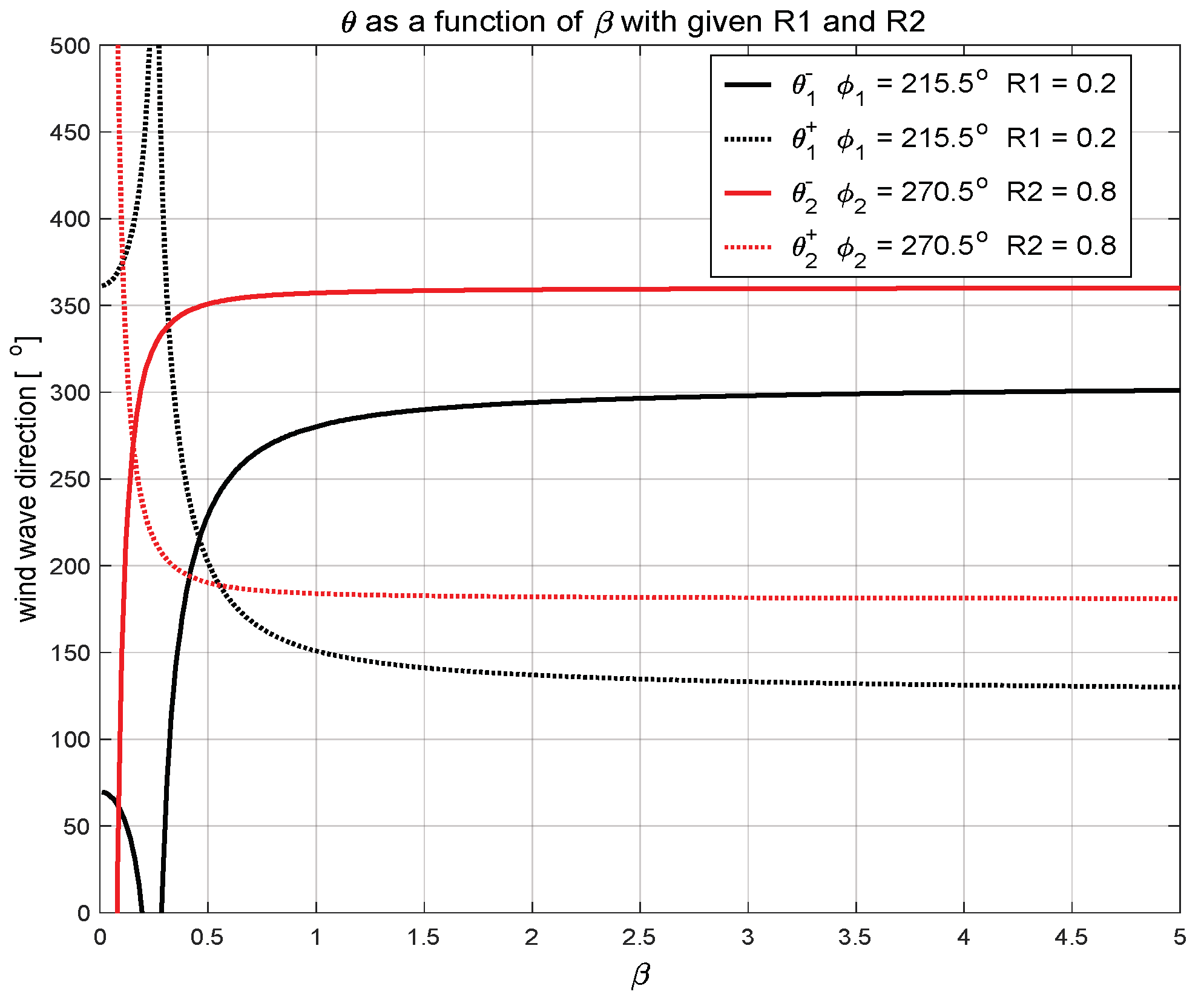
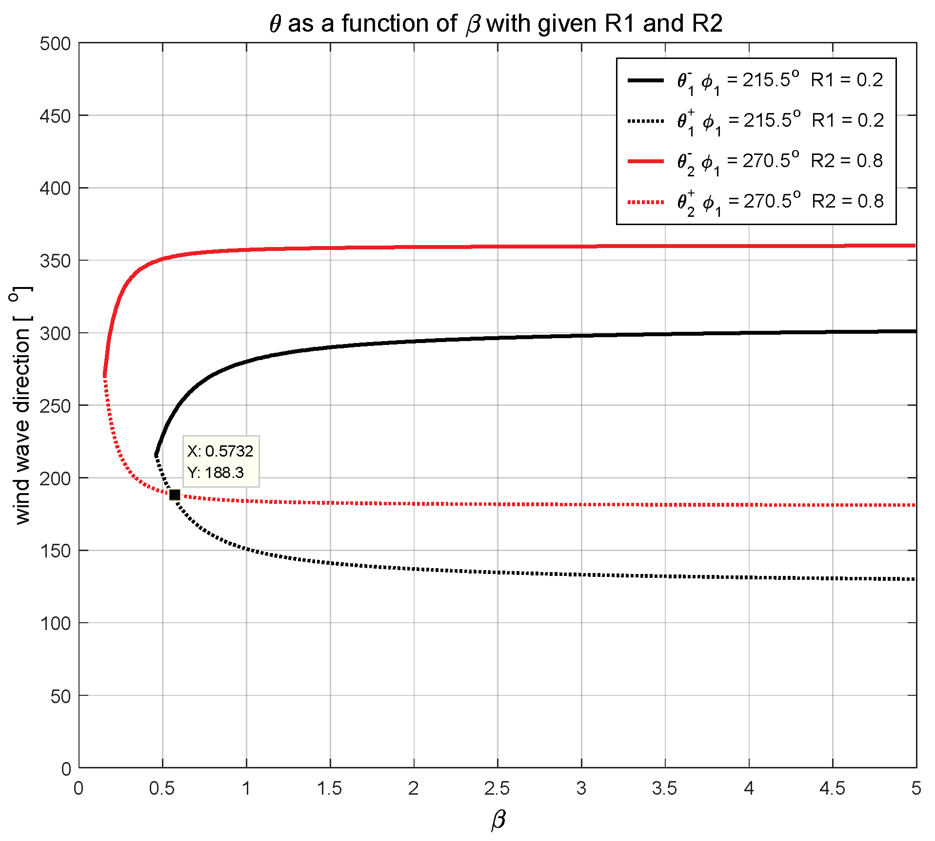
2.1. Power Ratio of a Radar’s First-Order Peaks and Wave Directional Distribution
2.2. Wind Direction Inversion from a Radar’s First-Order Backscatter
2.3. Proposed Pattern-Fitting Method for Wind Direction Inversion
2.4. Wind Direction and Wavelength of Resonant Waves
2.5. Wind Direction Inversion and Wind Speed
3. Experiments and Results
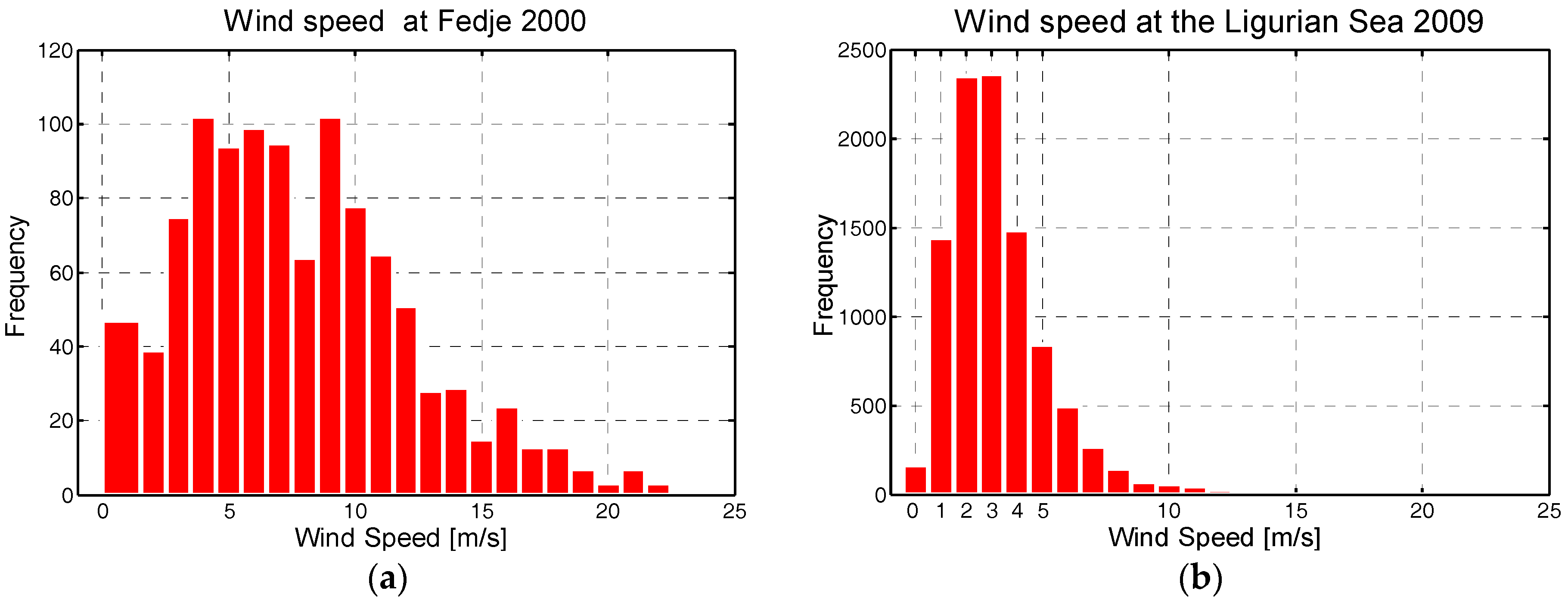
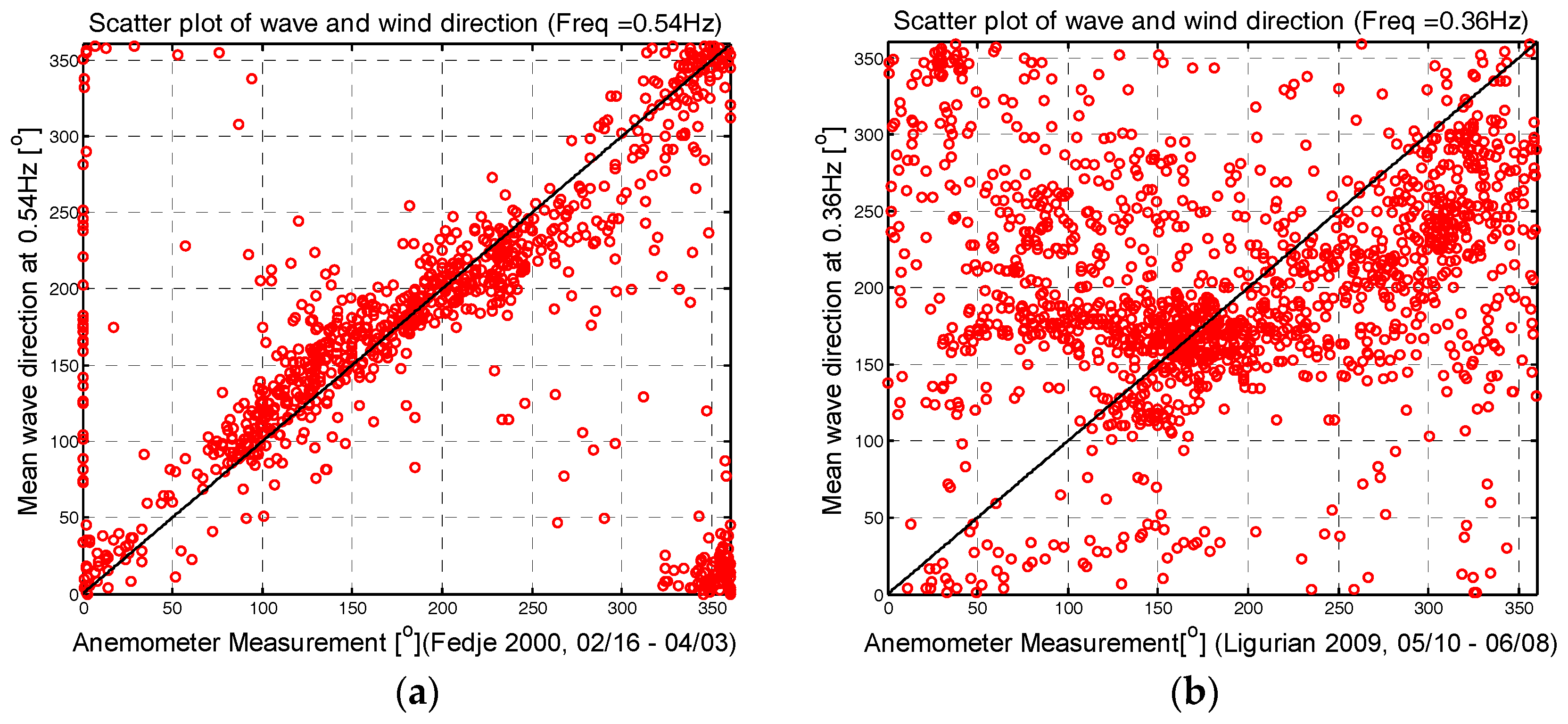
3.1. Introduction to Radar Experiments and Wind Conditions
3.2. Result of Experiments
4. Conclusions
Author Contributions
Funding
Acknowledgments
Conflicts of Interest
References
- Crombie, D.D. Doppler spectrum of sea echo at 13.56 mcs. Nature 1955, 4459, 681–682. [Google Scholar] [CrossRef]
- Long, A.E.; Trizna, D.B. Measurements and preliminary interpretation of hf radar Doppler spectra from the sea-echo of an atlantic storm. NRL Rep. 1972, 7456. [Google Scholar]
- Stewart, R.H.; Barnum, J.R. Radio measurements of oceanic winds at long ranges: An evaluation. Radio Sci. 1975, 10, 853–857. [Google Scholar] [CrossRef]
- Tyler, G.L.; Teague, C.C.; Stewart, R.H.; Peterson, A.M.; Munk, W.H.; Joy, J.W. Wave directional spectra from synthetic aperture observations of radio scatter. Deep Sea Res. Oceanogr. Abstr. 1974. [Google Scholar] [CrossRef]
- Zeng, Y.; Zhou, H.; Lai, Y.; Wen, B. Wind-direction mapping with a modified wind spreading function by broad-beam high-frequency radar. IEEE Geosci. Remote Sens. Lett. 2018, 15, 679–683. [Google Scholar] [CrossRef]
- Donelan, M.A.; Hamilton, J.; Hui, W.H. Directional spectra of wind-generated waves. Phil. Trans. R. Soc. Lond. 1985, 315, 509–562. [Google Scholar] [CrossRef]
- Gurgel, K.W.; Essen, H.H.; Schlick, T. An empirical method to derive ocean waves from second-order Bragg scattering: Prospects and limitations. IEEE J. Ocean. Eng. 2006, 31, 804–811. [Google Scholar] [CrossRef]
- Heron, M.L. Applying a unified directional wave spectrum to the remote sensing of wind wave directional spreading. Can. J. Remote Sens. 2002, 28, 346–353. [Google Scholar] [CrossRef]
- Heron, M.L.; Prytz, A. Wave height and wind direction from the hf coastal ocean surface radar. Can. J. Remote Sens. 2002, 28, 385–393. [Google Scholar] [CrossRef]
- Huang, W.; Gill, E.; Wu, S.; Wen, B.; Yang, Z.; Hou, J. Measuring surface wind direction by monostatic HF ground-wave radar at the eastern China sea. IEEE J. Ocean. Eng. 2004, 29, 1032–1037. [Google Scholar] [CrossRef]
- Chu, X.; Zhang, J.; Ji, Y.; Wang, Y.; Yang, L. Extraction of wind direction from the hf hybrid sky-surface wave radar sea echoes. IEEE Aerosp. Electron. Syst. Mag. 2018, 33, 42–47. [Google Scholar] [CrossRef]
- Shen, W.; Gurgel, K.W.; Voulgaris, G.; Schlick, T.; Stammer, D. Wind-speed inversion from HF radar first-order backscatter signal. Ocean. Dyn. 2012, 62, 105–121. [Google Scholar] [CrossRef]
- Hisaki, Y. Sea Surface Wind Correction Using HF Ocean Radar and Its Impact on Coastal Wave Prediction. J. Atmos. Ocean. Technol. 2017, 34, 2001–2020. [Google Scholar] [CrossRef]
- Kirincich, A. Toward real-time, remote observations of the coastal wind resource using high-frequency radar. Mar. Technol. Soc. J. 2013, 47, 206–217. [Google Scholar] [CrossRef]
- Kirincich, A. Remote Sensing of the Surface Wind Field over the Coastal Ocean via Direct Calibration of HF Radar Backscatter Power. J. Atmos. Ocean. Technol. 2016, 33, 1377–1392. [Google Scholar] [CrossRef] [Green Version]
- Zeng, Y.; Zhou, H.; Roarty, H.; Wen, B. Wind Speed Inversion in High Frequency Radar Based on Neural Network. Int. J. Antennas Propag. 2016, 2016. [Google Scholar] [CrossRef]
- Li, X.; Yu, C.; Su, F.; Quan, T.; Chu, X.; Wang, S. Significant wave height extraction using a low-frequency HFSWR system under low sea state. IET Radar Sonar Navig. 2018, 12, 671–677. [Google Scholar] [CrossRef]
- Halverson, M.; Pawlowicz, R.; Chavanne, C. Dependence of 25-MHz HF Radar Working Range on Near-Surface Conductivity, Sea State, and Tides. J. Atmos. Ocean. Technol. 2017, 34, 447–462. [Google Scholar] [CrossRef]
- Dexter, P.E.; Theodorides, S. Surface wind speed extraction from hf sky-wave radar doppler spectra. Radio Sci. 1982, 17, 643–652. [Google Scholar] [CrossRef]
- Hasselmann, D.E.; Dunckel, M.; Ewing, J.A. Directional wave spectra observing during jonswap 1973. J. Phys. Oceanogr. 1980, 10, 1264–1280. [Google Scholar] [CrossRef]
- Barrick, D.E. First-order theory and analysis of mf/hf/vhf surface from the sea. IEEE Trans. Atennas Propag. 1972, 20, 2–10. [Google Scholar] [CrossRef]
- Robson, R.E. Simplified theory of first- and second-order scattering of hf radio waves from the sea. Radio Sci. 1984, 19, 1499–1504. [Google Scholar] [CrossRef]
- Nagai, K. Diffraction of the irregular sea due to breakwaters. Coast. Eng. Japan. JSCE 1972, 15, 59–67. [Google Scholar] [CrossRef]
- Borgman, L.E. Directional spectrum estimation for the sxy gauges. Tech. Rep. Coast. Eng. Res. Center Vicksburg 1984. [Google Scholar]
- Longuet-Higgins, M.S.; Cartwright, D.E.; Smith, N.D. Observations of the directional spectrum of sea waves using the motions of a floating buoy. In Ocean Wave Spectra; Prentice-Hall Inc.: Upper Saddle River, NJ, USA, 1963; pp. 111–136. [Google Scholar]
- Mitsuyasu, H.; Tasai, F.; Suhara, T.; Mizuno, S.; Ohkusu, M.; Honda, T.; Rikiishi, K. Observations of the directional spectrum of ocean waves using a cloverleaf buoy. J. Phys. Oceanogr. 1975, 5, 750–761. [Google Scholar] [CrossRef]
- Chu, X.L.; Zhang, J.; Wang, S.Y.; Ji, Y.; et al. A Comparison of Algorithms for Extracting Wind Direction from the Monostatic HF Radar Sea Echoes. In Proceedings of the 2015 International Conference on Electronic Science and Automation Control, Zhengzhou, China, 15–16 August 2015. [Google Scholar]


| R1, R2 | Curves with a Cross-Point | Conditions | |
|---|---|---|---|
| R2 < R1 < 1 | 1 | ||
| R1 < R2 < 1 | 1 | ||
| R1 < 1, R2 < 1 | / |
| R1 and R2 | ||
|---|---|---|
| ; | ||
| ; | ||
| ; | ||
| ; | ||
| ; | ||
| ; | ||
| ; | ||
| ; | ||
| [1] | [2] |
| Radar Frequency (MHz) | Bragg Wave Frequency (Hz) | Bragg Wave Length (m) |
|---|---|---|
| 12 | 0.3534 | 12.5 |
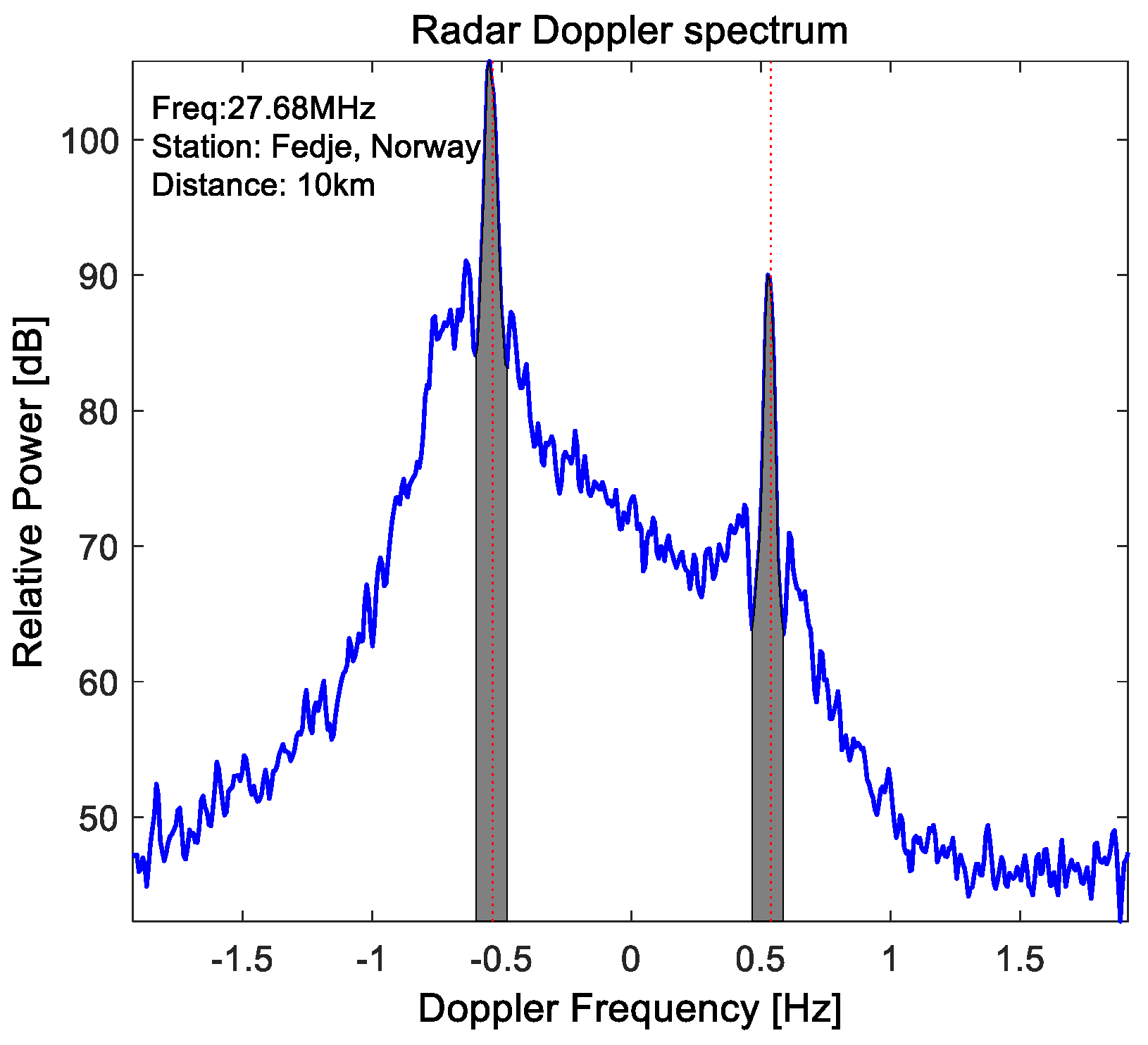
| 27.68 | 0.5368 | 5.419 |
| RMS Error for Wind Direction Measurements (°) | ||||
|---|---|---|---|---|
| Comparison of inversion method | Wind Speed (m/s) | Wind Speed Range (m/s) | ||
| U > 3 | 0 < U 3 | 3 < U 10 | U > 10 | |
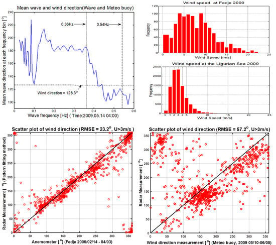
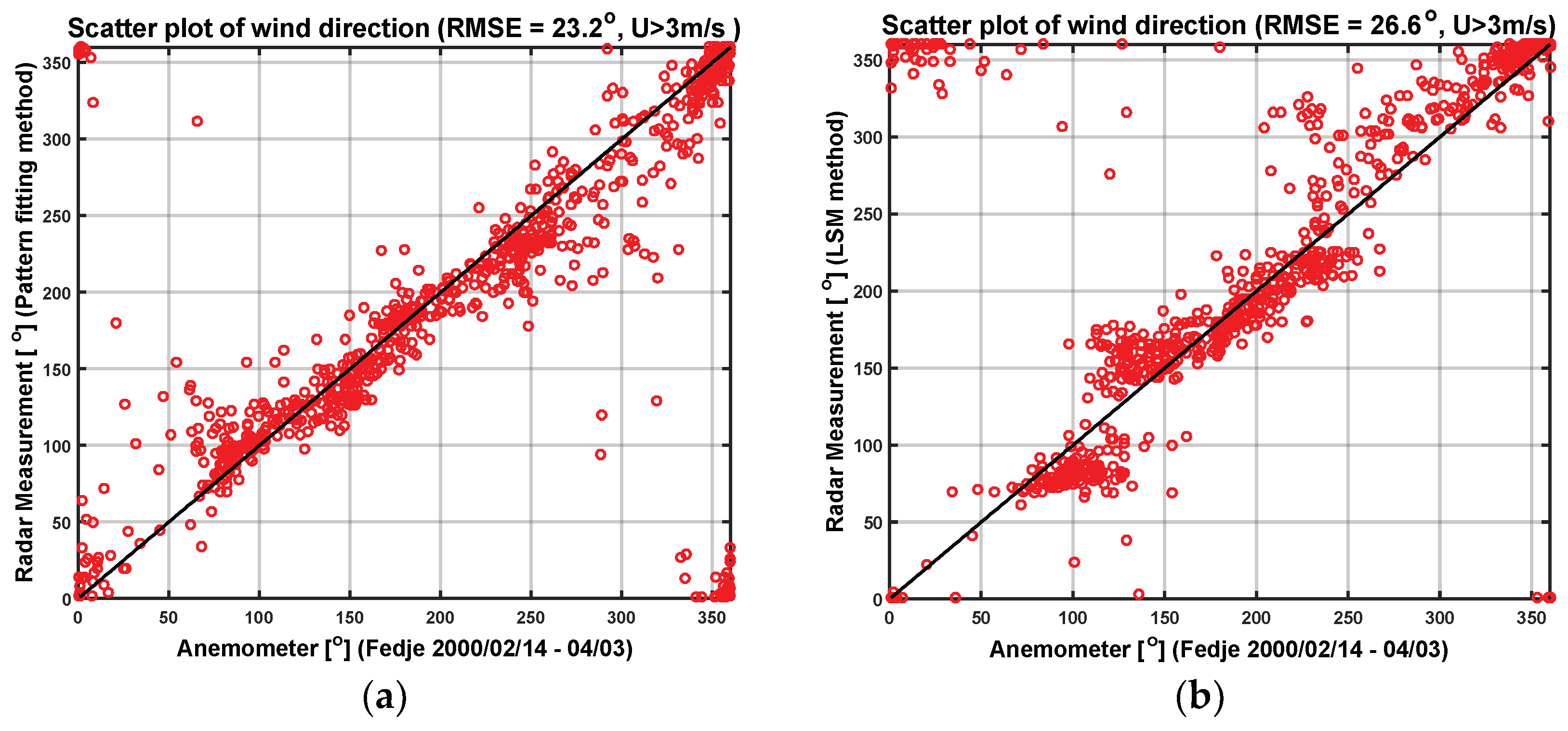
| Pattern-fitting method | 23.2 | 72.5 | 25.8 | 12.5 |
| LSM method | 26.6 | 75.9 | 29.5 | 14.8 |
| RMS Error for Wind Direction Measurements (°) | ||||
|---|---|---|---|---|
| Comparison of inversion method | Wind speed (m/s) | Wind speed range (m/s) | ||
| U > 3 | 0 < U 3 | 3 < U 10 | U > 10 | |
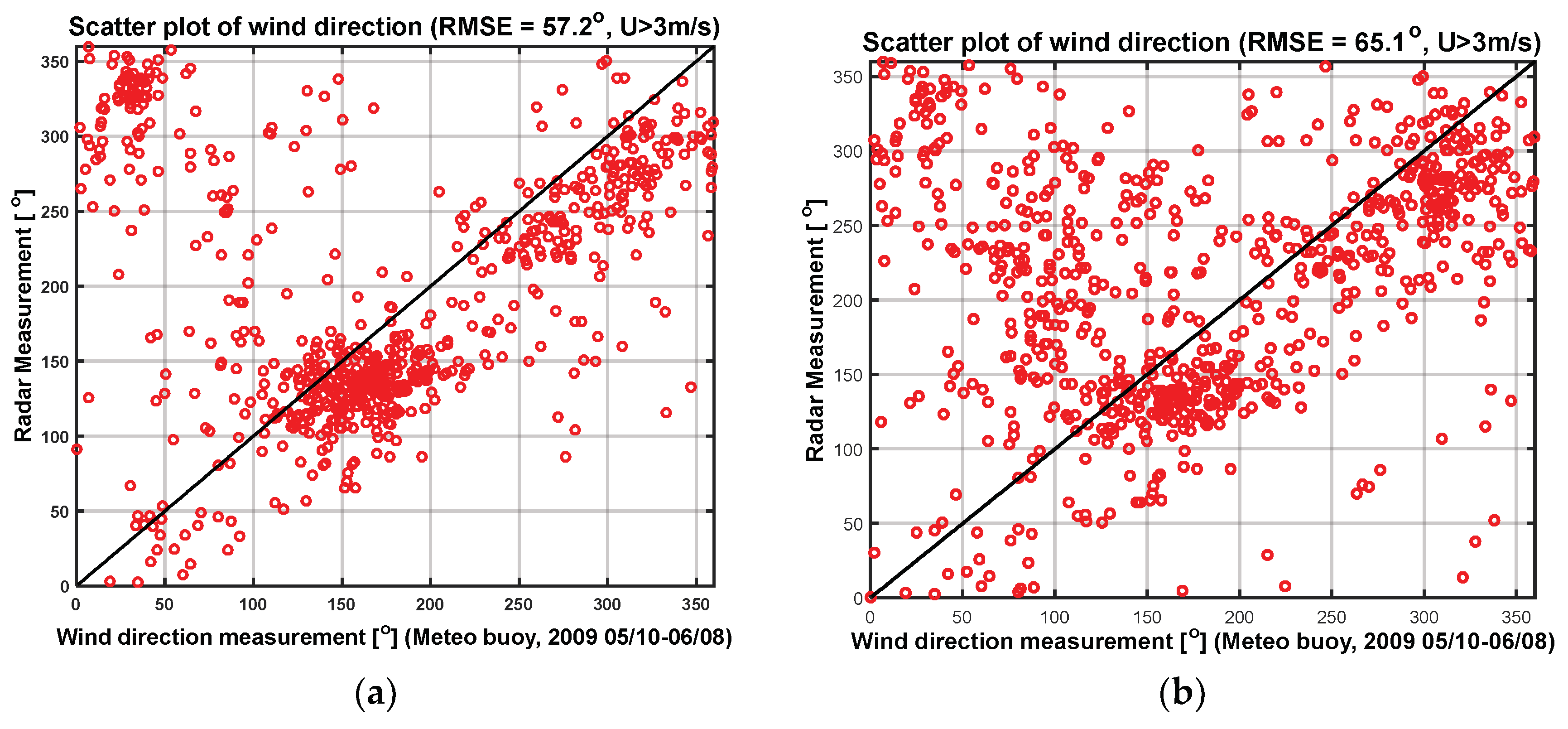
| Pattern-fitting method | 57.2 | 80.3 | 57.6 | 20.4 |
| LSM method | 65.1 | 84.6 | 64.7 | 24.1 |
© 2018 by the authors. Licensee MDPI, Basel, Switzerland. This article is an open access article distributed under the terms and conditions of the Creative Commons Attribution (CC BY) license (http://creativecommons.org/licenses/by/4.0/).
Share and Cite
Shen, W.; Gurgel, K.-W. Wind Direction Inversion from Narrow-Beam HF Radar Backscatter Signals in Low and High Wind Conditions at Different Radar Frequencies. Remote Sens. 2018, 10, 1480. https://0-doi-org.brum.beds.ac.uk/10.3390/rs10091480
Shen W, Gurgel K-W. Wind Direction Inversion from Narrow-Beam HF Radar Backscatter Signals in Low and High Wind Conditions at Different Radar Frequencies. Remote Sensing. 2018; 10(9):1480. https://0-doi-org.brum.beds.ac.uk/10.3390/rs10091480
Chicago/Turabian StyleShen, Wei, and Klaus-Werner Gurgel. 2018. "Wind Direction Inversion from Narrow-Beam HF Radar Backscatter Signals in Low and High Wind Conditions at Different Radar Frequencies" Remote Sensing 10, no. 9: 1480. https://0-doi-org.brum.beds.ac.uk/10.3390/rs10091480