Remotely Estimating Beneficial Arthropod Populations: Implications of a Low-Cost Small Unmanned Aerial System

Abstract
:
1. Introduction
2. Materials and Methods
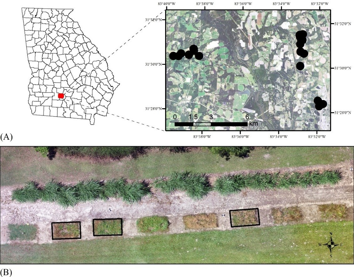
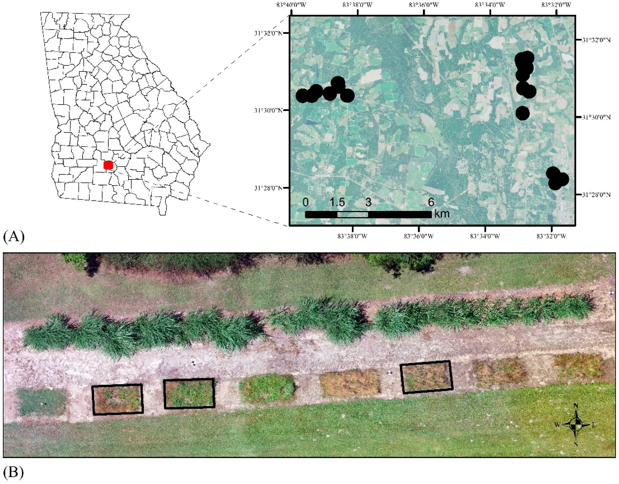
2.1. Field Sites
2.2. UAV Mission Preparation
2.3. Image Acquisition
2.4. Image Processing and Analysis
2.5. Vegetation and Arthropod Sampling
2.6. Statistical Analysis
3. Results
4. Discussion
5. Conclusions
Author Contributions
Funding
Acknowledgments
Conflicts of Interest
References
- Gurr, G.M.; Wratten, S.D.; Landis, D.A.; You, M. Habitat management to suppress pest populations: Progress and prospects. Annu. Rev. Entomol. 2017, 62, 91–109. [Google Scholar] [CrossRef] [PubMed]
- Landis, D.A. Designing agricultural landscapes for biodiversity-based ecosystem services. Basic Appl. Ecol. 2017, 18, 1–12. [Google Scholar] [CrossRef]
- Tschumi, M.; Albrecht, M.; Bärtschi, C.; Collatz, J.; Entling, M.H.; Jacot, K. Perennial, species-rich wildflower strips enhance pest control and crop yield. Agric. Ecosyst. Environ. 2016, 220, 97–103. [Google Scholar] [CrossRef]
- Tschumi, M.; Albrecht, M.; Collatz, J.; Dubsky, V.; Entling, M.H.; Najar-Rodriguez, A.J.; Jacot, K. Tailored flower strips promote natural enemy biodiversity and pest control in potato crops. J. Appl. Ecol. 2016, 53, 1169–1176. [Google Scholar] [CrossRef]
- Hatt, S.; Lopes, T.; Boeraeve, F.; Chen, J.; Francis, F. Pest regulation and support of natural enemies in agriculture: Experimental evidence of within field wildflower strips. Ecol. Eng. 2017, 98, 240–245. [Google Scholar] [CrossRef] [Green Version]
- Balzan, M.V.; Bocci, G.; Moonen, A.C. Utilisation of plant functional diversity in wildflower strips for the delivery of multiple agroecosystem services. Entomol. Exp. Appl. 2016, 158, 304–319. [Google Scholar] [CrossRef] [Green Version]
- Martin, E.A.; Seo, B.; Park, C.R.; Reineking, B.; Steffan-Dewenter, I. Scale-dependent effects of landscape composition and configuration on natural enemy diversity, crop herbivory, and yields. Ecol. Appl. 2016, 26, 448–462. [Google Scholar] [CrossRef] [PubMed]
- Fiedler, A.K.; Landis, D.A. Plant characteristics associated with natural enemy abundance at Michigan native plants. Environ. Entomol. 2007, 36, 878–886. [Google Scholar] [CrossRef] [PubMed]
- Tuell, J.K.; Fiedler, A.K.; Landis, D.; Isaacs, R. Visitation by wild and managed bees (Hymenoptera: Apoidea) to Eastern U.S. Native plants for use in conservation programs. Environ. Entomol. 2008, 37, 707–718. [Google Scholar] [CrossRef]
- Thorp, K.; Dierig, D. Color image segmentation approach to monitor flowering in lesquerella. Ind. Crop. Prod. 2011, 34, 1150–1159. [Google Scholar] [CrossRef]
- Fritz, S.; See, L.; McCallum, I.; You, L.; Bun, A.; Moltchanova, E.; Duerauer, M.; Albrecht, F.; Schill, C.; Perger, C. Mapping global cropland and field size. Glob. Chang. Biol. 2015, 21, 1980–1992. [Google Scholar] [CrossRef] [PubMed] [Green Version]
- Eberhardt, I.D.R.; Schultz, B.; Rizzi, R.; Sanches, I.D.A.; Formaggio, A.R.; Atzberger, C.; Mello, M.P.; Immitzer, M.; Trabaquini, K.; Foschiera, W.; et al. Cloud cover assessment for operational crop monitoring systems in tropical areas. Remote Sens. 2016, 8, 219. [Google Scholar] [CrossRef]
- Anderson, K.; Gaston, K.J. Lightweight unmanned aerial vehicles will revolutionize spatial ecology. Front. Ecol. Environ. 2013, 11, 138–146. [Google Scholar] [CrossRef] [Green Version]
- Cruzan, M.B.; Weinstein, B.G.; Grasty, M.R.; Kohrn, B.F.; Hendrickson, E.C.; Arredondo, T.M.; Thompson, P.G. Small unmanned aerial vehicles (micro-uavs, drones) in plant ecology. Appl. Plant Sci. 2016, 4, 1600041. [Google Scholar] [CrossRef] [PubMed]
- Zhang, C.; Kovacs, J.M. The application of small unmanned aerial systems for precision agriculture: A review. Precis. Agric. 2012, 13, 693–712. [Google Scholar] [CrossRef]
- Hardin, P.J.; Hardin, T.J. Small-scale remotely piloted vehicles in environmental research. Geogr. Compass 2010, 4, 1297–1311. [Google Scholar] [CrossRef]
- Lelong, C.C.; Burger, P.; Jubelin, G.; Roux, B.; Labbé, S.; Baret, F. Assessment of unmanned aerial vehicles imagery for quantitative monitoring of wheat crop in small plots. Sensors 2008, 8, 3557–3585. [Google Scholar] [CrossRef] [PubMed]
- Rango, A.; Laliberte, A.; Herrick, J.E.; Winters, C.; Havstad, K.; Steele, C.; Browning, D. Unmanned aerial vehicle-based remote sensing for rangeland assessment, monitoring, and management. J. Appl. Remote Sens. 2009, 3, 033542. [Google Scholar] [CrossRef]
- Biradar, B.V.; Shrikhande, S.P. Flower detection and counting using morphological and segmentation technique. Int. J. Comput. Sci. Inf. Technol. 2015, 6, 2498–2501. [Google Scholar]
- Siraj, F.; Salahuddin, M.A.; Yusof, S.A.M. Digital image classification for malaysian blooming flower. In Proceedings of the 2010 Second International Conference on Computational Intelligence, Modelling and Simulation (CIMSiM), Tuban, Indonesia, 28–30 September 2010; pp. 33–38. [Google Scholar]
- Thorp, K.; Wang, G.; Badaruddin, M.; Bronson, K. Lesquerella seed yield estimation using color image segmentation to track flowering dynamics in response to variable water and nitrogen management. Ind. Crop. Prod. 2016, 86, 186–195. [Google Scholar] [CrossRef]
- Swain, K.C.; Thomson, S.J.; Jayasuriya, H.P. Adoption of an unmanned helicopter for low-altitude remote sensing to estimate yield and total biomass of a rice crop. Trans. ASABE 2010, 53, 21–27. [Google Scholar] [CrossRef]
- Hunt, E.R.; Cavigelli, M.; Daughtry, C.S.; Mcmurtrey, J.E.; Walthall, C.L. Evaluation of digital photography from model aircraft for remote sensing of crop biomass and nitrogen status. Precis. Agric. 2005, 6, 359–378. [Google Scholar] [CrossRef]
- Agüera, F.; Carvajal, F.; Pérez, M. Measuring sunflower nitrogen status from an unmanned aerial vehicle-based system and an on the ground device. Int. Arch. Photogramm. Remote Sens. Spat. Inf. Sci. 2011, 38, 33–37. [Google Scholar] [CrossRef]
- Lehmann, J.R.K.; Nieberding, F.; Prinz, T.; Knoth, C. Analysis of unmanned aerial system-based images in forestry—A new perspective to monitor pest infestation levels. Forests 2015, 6, 594–612. [Google Scholar] [CrossRef] [Green Version]
- Näsi, R.; Honkavaara, E.; Lyytikäinen-Saarenmaa, P.; Blomqvist, M.; Litkey, P.; Hakala, T.; Viljanen, N.; Kantola, T.; Tanhuanpää, T.; Holopainen, M. Using uav-based photogrammetry and hyperspectral imaging for mapping bark beetle damage at tree-level. Remote Sens. 2015, 7, 15467–15493. [Google Scholar] [CrossRef]
- Cunliffe, A.M.; Brazier, R.E.; Anderson, K. Ultra-fine grain landscape-scale quantification of dryland vegetation structure with drone-acquired structure-from-motion photogrammetry. Remote Sens. Environ. 2016, 183, 129–143. [Google Scholar] [CrossRef] [Green Version]
- Calvario, G.; Sierra, B.; Alarcón, T.E.; Hernandez, C.; Dalmau, O. A multi-disciplinary approach to remote sensing through low-cost uavs. Sensors 2017, 17, 1411. [Google Scholar] [CrossRef] [PubMed]
- Fang, S.; Tang, W.; Peng, Y.; Gong, Y.; Dai, C.; Chai, R.; Liu, K. Remote estimation of vegetation fraction and flower fraction in oilseed rape with unmanned aerial vehicle data. Remote Sens. 2016, 8, 416. [Google Scholar] [CrossRef]
- Severtson, D.; Callow, N.; Flower, K.; Neuhaus, A.; Olejnik, M.; Nansen, C. Unmanned aerial vehicle canopy reflectance data detects potassium deficiency and green peach aphid susceptibility in canola. Precis. Agric. 2016, 17, 659–677. [Google Scholar] [CrossRef]
- Müllerová, J.; Bartaloš, T.; Brůna, J.; Dvořák, P.; Vítková, M. Unmanned aircraft in nature conservation: An example from plant invasions. Int. J. Remote Sens. 2017, 38, 2177–2198. [Google Scholar] [CrossRef]
- Michez, A.; Piégay, H.; Jonathan, L.; Claessens, H.; Lejeune, P. Mapping of riparian invasive species with supervised classification of unmanned aerial system (UAS) imagery. Int. J. Appl. Earth Obs. Geoinf. 2016, 44, 88–94. [Google Scholar] [CrossRef]
- Hill, D.J.; Tarasoff, C.; Whitworth, G.E.; Baron, J.; Bradshaw, J.L.; Church, J.S. Utility of unmanned aerial vehicles for mapping invasive plant species: A case study on yellow flag Iris (Iris pseudacorus L.). Int. J. Remote Sens. 2017, 38, 2083–2105. [Google Scholar] [CrossRef]
- Carl, C.; Landgraf, D.; van der Maaten-Theunissen, M.; Biber, P.; Pretzsch, H. Robinia pseudoacacia L. flowers analyzed by using Unmanned Aerial Vehicle (UAV). Remote Sens. 2017, 9, 1091. [Google Scholar] [CrossRef]
- Lino, A.C.L.; Sanches, J.; Moraes, G.; Dias-Tagliacozzo, I.; Augusto, F.; LIMA, B.; Nascimento, T.S. Flower classification supported by digital imaging techniques. J. Inf. Technol. Agric. 2011, 4, 1–6. [Google Scholar]
- Xavier, S.S.; Olson, D.M.; Coffin, A.W.; Strickland, T.C.; Schmidt, J.M. Perennial grass and native wildflowers: A synergistic approach to habitat management. Insects 2017, 8, 104. [Google Scholar] [CrossRef] [PubMed]
- Lillesand, T.M.; Kiefer, R.W.; Chipman, J.W. Remote Sensing and Image Interpretation; Wiley: New York, NY, USA, 2004; Volume 5. [Google Scholar]
- Agisoft. Agisoft Photoscan User Manual: Professional Edition, version 1.1; Agisoft, L.L.C.: St. Petersburg, Russia, 2014. [Google Scholar]
- Foody, G.M.; Campbell, N.; Trodd, N.; Wood, T. Derivation and applications of probabilistic measures of class membership from the maximum-likelihood classification. Photogramm. Eng. Remote Sens. 1992, 58, 1335–1341. [Google Scholar]
- Environmental System Research Institute (ESRI). Arcgis Desktop: Release 10.5.1; Environmental System Research Institute: Redlands, CA, USA, 2017. [Google Scholar]
- Fitzgerald, R.; Lees, B. Assessing the classification accuracy of multisource remote sensing data. Remote Sens. Environ. 1994, 47, 362–368. [Google Scholar] [CrossRef]
- RCoreTeam. R: A Language and Environment for Statistical Computing; R Foundation for Statistical Computing: Vienna, Austria, 2017. [Google Scholar]
- Szigeti, V.; Kőrösi, Á.; Harnos, A.; Nagy, J.; Kis, J. Measuring floral resource availability for insect pollinators in temperate grasslands—A review. Ecol. Entomol. 2016, 41, 231–240. [Google Scholar] [CrossRef]
- Wakakuwa, M.; Stavenga, D.G.; Arikawa, K. Spectral organization of ommatidia in flower-visiting insects†. Photochem. Photobiol. 2007, 83, 27–34. [Google Scholar] [CrossRef] [PubMed]
- Venturini, E.M.; Drummond, F.A.; Hoshide, A.K.; Dibble, A.C.; Stack, L.B. Pollination reservoirs for wild bee habitat enhancement in cropping systems: A review. Agroecol. Sustain. Food Syst. 2017, 41, 101–142. [Google Scholar] [CrossRef]
- Williams, N.M.; Ward, K.L.; Pope, N.; Isaacs, R.; Wilson, J.; May, E.A.; Ellis, J.; Daniels, J.; Pence, A.; Ullmann, K. Native wildflower plantings support wild bee abundance and diversity in agricultural landscapes across the united states. Ecol. Appl. 2015, 25, 2119–2131. [Google Scholar] [CrossRef] [PubMed]
- Szigeti, V.; Kőrösi, Á.; Harnos, A.; Nagy, J.; Kis, J. In Comparing two methods for estimating floral resource availability for insect pollinators in semi-natural habitats. Ann. Soc. Entomol. Fr. (NS) 2016, 52, 289–299. [Google Scholar] [CrossRef]
- Hatt, S.; Boeraeve, F.; Artru, S.; Dufrêne, M.; Francis, F. Spatial diversification of agroecosystems to enhance biological control and other regulating services: An agroecological perspective. Sci. Total. Environ. 2018, 621, 600–611. [Google Scholar] [CrossRef] [PubMed] [Green Version]
- Tscharntke, T.; Karp, D.S.; Chaplin-Kramer, R.; Batáry, P.; DeClerck, F.; Gratton, C.; Hunt, L.; Ives, A.; Jonsson, M.; Larsen, A. When natural habitat fails to enhance biological pest control–five hypotheses. Biol. Conserv. 2016, 204, 449–458. [Google Scholar] [CrossRef]
- McCabe, E.; Loeb, G.; Grab, H. Responses of crop pests and natural enemies to wildflower borders depends on functional group. Insects 2017, 8, 73. [Google Scholar] [CrossRef] [PubMed]
- Shackelford, G.; Steward, P.R.; Benton, T.G.; Kunin, W.E.; Potts, S.G.; Biesmeijer, J.C.; Sait, S.M. Comparison of pollinators and natural enemies: A meta-analysis of landscape and local effects on abundance and richness in crops. Biol. Rev. 2013, 88, 1002–1021. [Google Scholar] [CrossRef] [PubMed]


| Flower Description | 8 May 2017 | 8 June 2017 | 10 July 2017 | 7 August 2017 | 18 September 2017 | |||||||||||
|---|---|---|---|---|---|---|---|---|---|---|---|---|---|---|---|---|
| Eden | Ameri | High | Eden | Ameri | High | Eden | Ameri | High | Eden | Ameri | High | Eden | Ameri | High | Total | |
| Gaillardia pulchella | 83 | 121 | 106 | 122 | 119 | 151 | 148 | 182 | 152 | 223 | 289 | 249 | 161 | 202 | 160 | 2468 |
| Rudbeckia hirta | 0 | 1 | 0 | 127 | 160 | 103 | 111 | 131 | 59 | 37 | 28 | 15 | 20 | 23 | 20 | 835 |
| Coreopsis lanceolata | 75 | 49 | 145 | 1 | 0 | 21 | 21 | 10 | 37 | 0 | 0 | 1 | 0 | 1 | 0 | 361 |
| Coreopsis tinctoria | 61 | 7 | 0 | 42 | 24 | 30 | 0 | 0 | 0 | 0 | 0 | 0 | 0 | 0 | 0 | 164 |
| Centaurea cyanus | 69 | 0 | 0 | 27 | 0 | 0 | 0 | 0 | 0 | 0 | 0 | 0 | 0 | 0 | 0 | 96 |
| Rudbeckia gloriosa | 0 | 0 | 0 | 0 | 0 | 0 | 19 | 32 | 0 | 0 | 21 | 0 | 1 | 0 | 0 | 73 |
| Phlox drummondi | 12 | 0 | 0 | 9 | 0 | 0 | 0 | 0 | 0 | 13 | 0 | 0 | 0 | 0 | 0 | 34 |
| Linum grandiflorum | 33 | 0 | 0 | 0 | 0 | 0 | 0 | 0 | 0 | 0 | 0 | 0 | 0 | 0 | 0 | 33 |
| Cosmos sulphureus | 0 | 0 | 0 | 0 | 0 | 0 | 0 | 0 | 0 | 11 | 0 | 0 | 4 | 0 | 0 | 15 |
| Linaria maroccana | 0 | 12 | 2 | 0 | 0 | 0 | 0 | 0 | 0 | 0 | 0 | 0 | 0 | 0 | 0 | 14 |
| Monarda citriodora | 0 | 0 | 0 | 3 | 0 | 6 | 0 | 0 | 1 | 0 | 0 | 0 | 0 | 0 | 0 | 10 |
| Cosmos bipinnatus | 3 | 0 | 0 | 0 | 0 | 0 | 0 | 0 | 0 | 0 | 0 | 0 | 0 | 0 | 0 | 3 |
| Oenothera lamarckiana | 0 | 0 | 0 | 0 | 0 | 0 | 0 | 0 | 0 | 0 | 1 | 0 | 0 | 0 | 0 | 1 |
| Total | 336 | 190 | 253 | 331 | 303 | 311 | 299 | 355 | 249 | 284 | 339 | 265 | 186 | 226 | 180 | 4107 |
| Predictor Variable | Response Variable | Estimate (±SE) | t-Value | R2c | p-Value |
|---|---|---|---|---|---|
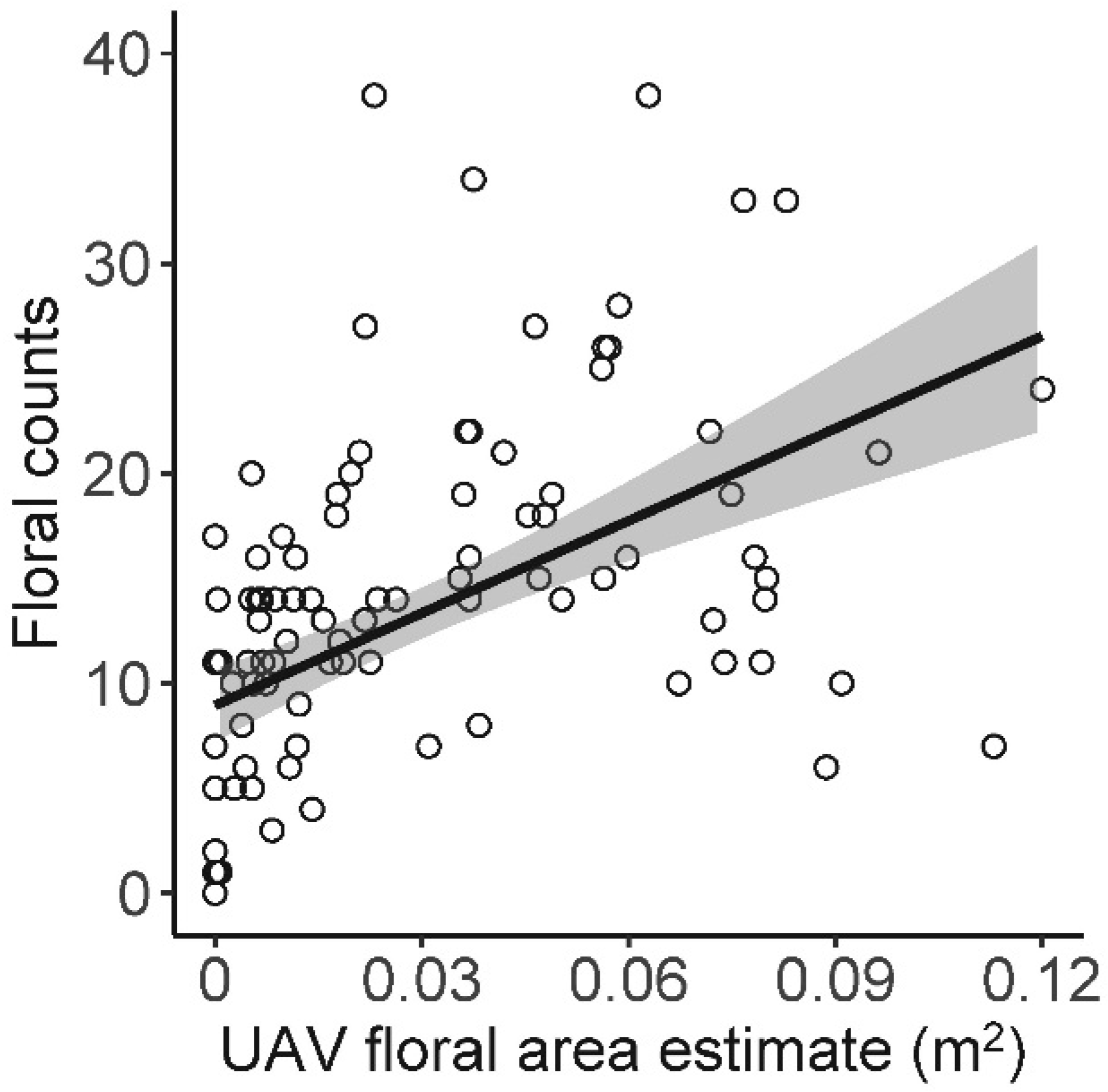
| UAV floral area | Floral counts | 13.127 (±2.53) | 5.192 | 0.26 | <0.001 |
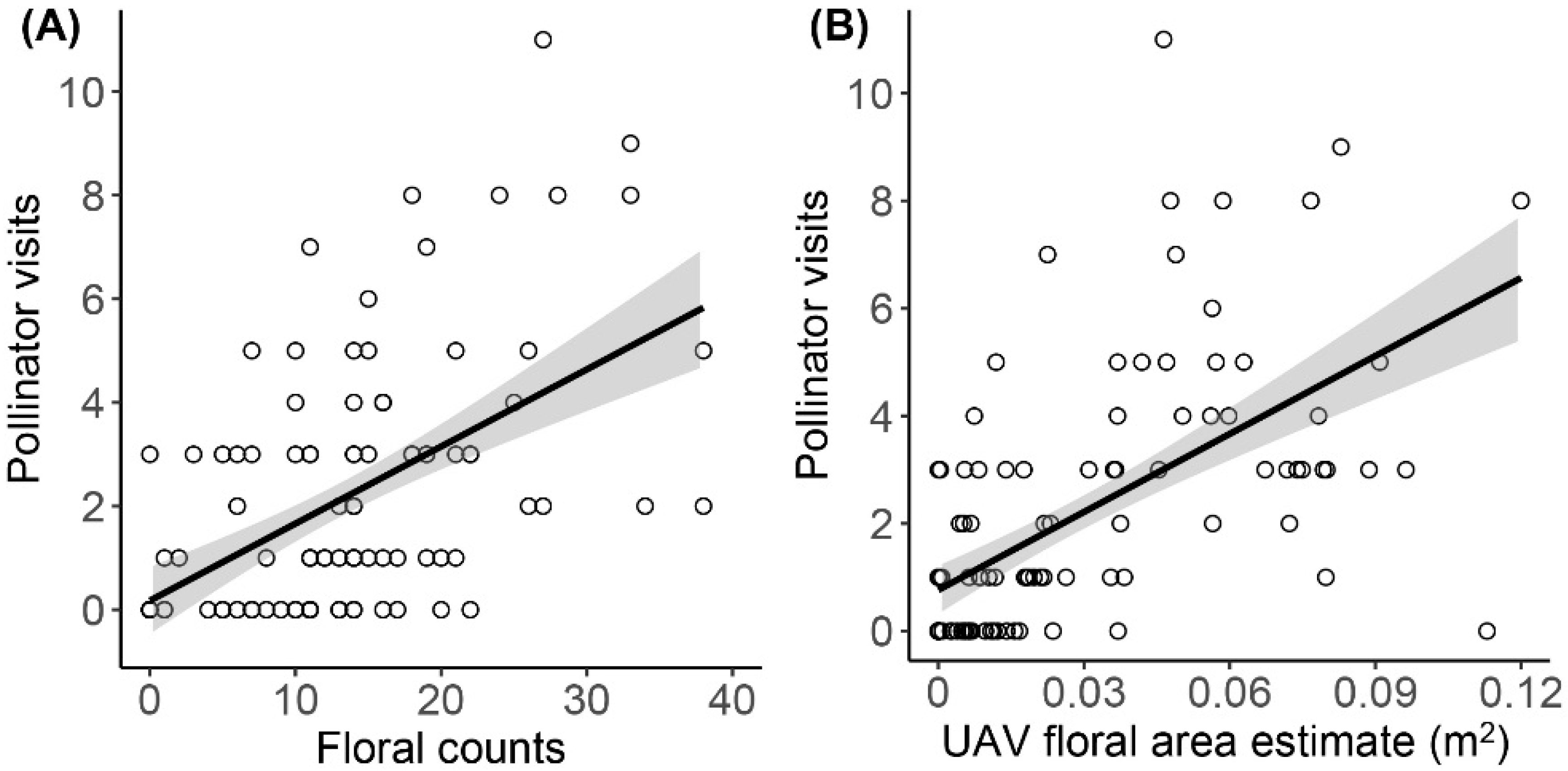
| Floral counts | Pollinator counts | 0.031 (±0.01) | 5.875 | 0.64 | <0.001 |
| UAV floral area | Pollinator counts | 6.340 (±1.81) | 3.502 | 0.51 | 0.0007 |
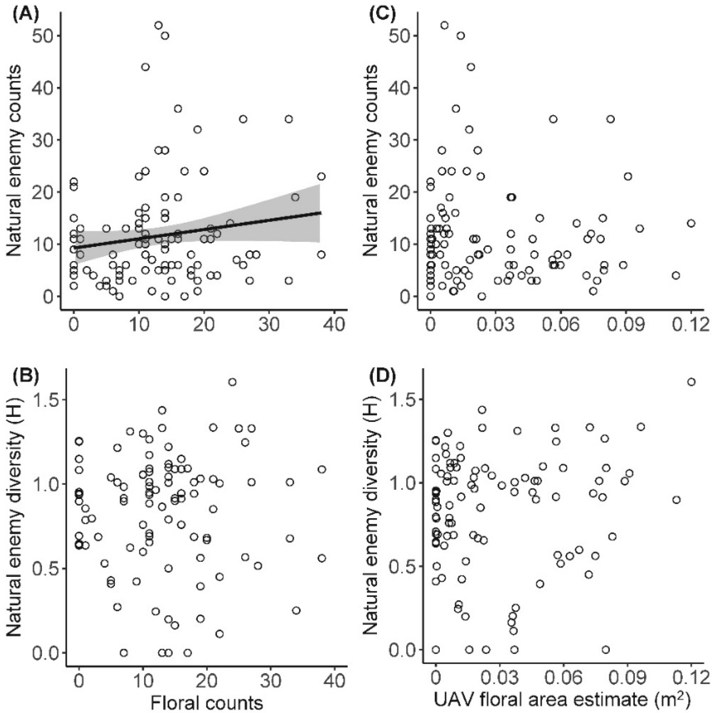
| Floral counts | Natural enemy counts | 0.019(±0.01) | 2.038 | 0.21 | 0.0443 |
| UAV floral area | Natural enemy counts | 2.785 (±2.71) | 1.025 | na | 0.3079 |
| Floral counts | Natural diversity | −0.000 (±0.002) | −0.072 | na | 0.9422 |
| UAV floral area | Natural diversity | 0.977 (±0.93) | 1.055 | na | 0.2939 |
| Date | Total | June | September |
|---|---|---|---|
| Araneae | 560 | 201, 3.72 (0.43) | 359, 6.65 (0.71) |
| Staphylinidae | 459 | 20, 0.37 (0.16) | 439, 8.13 (2.11) |
| Parasitica | 82 | 28, 0.52 (0.16) | 54, 1.00 (0.22) |
| Carabidae | 39 | 36, 0.67 (0.18) | 3, 0.06 (0.04) |
| Anthocoridae | 26 | 18, 0.33 (0.11) | 8, 0.15 (0.07) |
| Reduviidae | 23 | 15, 0.28 (0.09) | 8, 0.15 (0.06) |
| Coccinellidae | 17 | 5, 0.09 (0.05) | 12, 0.22 (0.09) |
| Braconidae | 10 | 1, 0.02 (0.02) | 9, 0.17 (0.05) |
| Ichneumonidae | 10 | 4, 0.07 (0.04) | 6, 0.11 (0.07) |
| Nabidae | 8 | 1, 0.02 (0.02) | 7, 0.13 (0.05) |
| Scoliidae | 3 | 3, 0.06 (0.03) | 0, 0 (0) |
| Tiphiidae | 3 | 3, 0.06 (0.04) | 0, 0 (0) |
| Sphecidae | 1 | 0, 0.00 (0.00) | 1, 0.02 (0.02) |
| Totals | 1241 | 335 | 906 |
© 2018 by the authors. Licensee MDPI, Basel, Switzerland. This article is an open access article distributed under the terms and conditions of the Creative Commons Attribution (CC BY) license (http://creativecommons.org/licenses/by/4.0/).
Share and Cite
Xavier, S.S.; Coffin, A.W.; Olson, D.M.; Schmidt, J.M. Remotely Estimating Beneficial Arthropod Populations: Implications of a Low-Cost Small Unmanned Aerial System. Remote Sens. 2018, 10, 1485. https://0-doi-org.brum.beds.ac.uk/10.3390/rs10091485
Xavier SS, Coffin AW, Olson DM, Schmidt JM. Remotely Estimating Beneficial Arthropod Populations: Implications of a Low-Cost Small Unmanned Aerial System. Remote Sensing. 2018; 10(9):1485. https://0-doi-org.brum.beds.ac.uk/10.3390/rs10091485
Chicago/Turabian StyleXavier, Shereen S., Alisa W. Coffin, Dawn M. Olson, and Jason M. Schmidt. 2018. "Remotely Estimating Beneficial Arthropod Populations: Implications of a Low-Cost Small Unmanned Aerial System" Remote Sensing 10, no. 9: 1485. https://0-doi-org.brum.beds.ac.uk/10.3390/rs10091485