Time-Varying SAR Interference Suppression Based on Delay-Doppler Iterative Decomposition Algorithm


1
School of Electronics and Information, Northwestern Polytechnical University, Xi’an 710072, China
2
School of Electronic Engineering, Xidian University, Xi’an 710071, China
3
School of Electrical and Electronic Engineering, The University of Adelaide, Adelaide, SA 5005, Australia
*
Author to whom correspondence should be addressed.
Remote Sens. 2018, 10(9), 1491; https://0-doi-org.brum.beds.ac.uk/10.3390/rs10091491
Submission received: 9 August 2018
/
Revised: 9 September 2018
/
Accepted: 14 September 2018
/
Published: 18 September 2018
(This article belongs to the Special Issue Radio Frequency Interference (RFI) in Microwave Remote Sensing)
Abstract
:Narrow-band interference (NBI) and Wide-band interference (WBI) are critical issues for synthetic aperture radar (SAR), which degrades the imaging quality severely. Since some complex signals can be modeled as linear frequency modulated (LFM) signals within a short time, LFM-WBI and NBI are mainly discussed in this paper. Due to its excellent energy concentration and useful properties (i.e., auto-terms pass through the origin of Delay-Doppler plane while cross-terms are away from it), a novel nonparametric interference suppression method using Delay-Doppler iterative decomposition algorithm is proposed. This algorithm consists of three stages. First, we present signal synthesis method (SSM) from ambiguity function (AF) and cross ambiguity function (CAF) based on the matrix rearrangement and eigenvalue decomposition. Compared with traditional SSM from Wigner distribution (WD), the proposed SSM can synthesize a signal faster and more accurately. Then, based on unique properties in Delay-Doppler domain, a mask algorithm is applied for interference identification and extraction using Radon and its inverse transformation. Finally, a signal iterative decomposition algorithm (IDA) is utilized to subtract the largest interference from the received signal one by one. After that, a well-focused SAR imagery is obtained by conventional imaging methods. The simulation and measured data results demonstrate that the proposed algorithm not only suppresses interference efficiently but also preserves the useful information as much as possible.
1. Introduction
Synthetic aperture radar (SAR) has become an important instrument for earth mapping and been widely utilized in both military surveillance and civilian exploration. However, well-focused SAR images are always prominently corrupted by untargeted interference caused by natural or man-made factors, especially the interferences whose frequencies fall into the frequency spectrum of useful signals [1,2]. Although the two-dimensional matched filter has an inherent ability in interference suppression, interferences with stronger power will defocus the image and degrade the imaging quality seriously [3,4].
Since the existence of interference would seriously degrade the quality of SAR imagery, interference detection and suppression have been paid increasing attention in the SAR community. In terms of ratio of the interference bandwidth to the useful signal, interference is generally categorized into two groups: narrowband interference (NBI, the ratio is smaller than 1%) and wideband interference (WBI, the ratio is greater than 1%). Compared with WBI, NBI is much easier to deal with. To obtain high-quality images, the NBI suppression algorithm can mainly be classified into two classes: parametric and non-parametric methods. In parametric approaches, the interferences are usually modeled as a summation of complex sinusoidal waves and their parameters, such as amplitude, frequency and phase, are estimated according to the least-mean square method [5,6,7] or maximum likelihood criteria [8]. Then, NBI can be reconstructed and subtracted from the received echoes. However, without prior knowledge, model mismatch will lead to an inaccurate estimated of the NBI and result in great degradation of the suppression performance. Additionally, it is difficult to obtain accurate high-dimensional parameters for non-stationary NBI. The other is the non-parametric method, including the notch filtering method [9,10,11,12,13] and the eigen-subspace projection method [14]. These methods avoid the complicated NBI modeling or multiparameter estimation. Notch filtering method is one of the most widely used interference suppression techniques in practice. Several excellent works are carried out on notch filter design, such as minimax optimization based IIR notch filter [10], Sliding DFT Phase Locking Scheme [11], adaptive filter [12,13], etc. They employ spectral estimation to distinguish the interference and design a proper filter to remove it in the frequency domain. These methods work based on the assumption that only a fraction of frequency bins of NBI are overlapped with that of useful signals. However, the frequency notch filtering method may cause the discontinuity of signal spectrum and further lead to the loss of useful signal. Thus, the signal-to-noise ratio (SNR) of the SAR image may degrade seriously. The eigen-subspace projection method projects echoes onto the interference subspace and the signal subspace, respectively. This approach has good performance for stationary interference suppression, while the suppression would lead to significant signal loss when time-varying interference exists. In addition, independent component analysis [15,16,17], empirical mode decomposition [18], sparsity and low-rank method [19], and the other excellent works [20,21,22] are proposed to cope with the time-varying interference with little useful signal loss.
By contrast, the WBI removal approaches are more complicated, since its bandwidth is large and occupies a large portion of the bandwidth of the useful SAR signal. The best choices of WBI suppression method are mainly based on multi-antenna, beamforming and space-time adaptive processing techniques, in which adaptive nulling is formed in the direction of the interference [23,24]. However, the hardware cost and complexity become more unaffordable, as the number of antennas increases [25]. Moreover, these methods perform poorly to counter jamming entering from the main lobe. Another WBI suppression framework is based on the analysis of the time–frequency (TF) properties of interference. TF based interference suppression methods can also be generally categorized into two groups: parametric and nonparametric approaches. In parametric methods, WBI is modeled as polynomial phase signal, whose parameters can be estimated by the fractional Fourier transform (FrFT) [26], polynomial phase transform (PPT) [27], high-order ambiguity function (HAF) [28], product high-order ambiguity function (PHAF) [29] and other time–frequency analysis-based parameter estimation methods [30,31,32,33]. Similar to the parametric methods in NBI suppression, model mismatch and parameter estimation error may lead to great degradation of the SAR image quality. Nonparametric methods mainly focus on TF characteristic analysis and TF filter design to remove the WBI and preserve the SAR signal. These methods usually assume that the WBI is concentrated in the TF domain. In this paper, we mainly focus on the linear frequency modulated (LFM) WBI (LFM-WBI), since some complex signal can be modeled as an LFM signal within a short time. Due to its good concentration at each time slice, short time Fourier transform (STFT) [34,35,36,37,38,39,40,41] has been shown as an effective tool for time-varying WBI suppression. The energy of interference concentrates in a few frequency bins in the instantaneous frequency spectrum at each time slice. However, its TF resolution varies with the bandwidth of signal, i.e., the larger the bandwidth is, the worse the TF resolution will be. Compared with STFT, Wigner distribution (WD) [42,43,44] is more effective for time-varying signal analysis due to its excellent energy concentration. For multiple components, WD’s bilinear transformation always produces unwanted cross-terms, which may severely impede auto-terms identification. Furthermore, the traditional signal synthesis method (SSM) from WD is quite time consuming and inaccurate. Ambiguity function (AF) [32,45] has the same energy concentration as WD does. Similarly, due to its bilinear transformation, AF will also suffer from the identifiability problem when dealing with multi-component signal. However, AF analysis tool has a useful property that auto-term passes through the origin of the AF plane and the cross-terms are away from it [32,45]. By making full use of this property, we propose an efficient interference suppression algorithm. First, we present an SSM from AF and cross AF (CAF). Then, a binary mask based on the Radon transform (RT) and its inverse transform is constructed for auto-terms extraction and cross-terms suppression, which overcomes the cross-terms identifiability issue in WD. Finally, an AF-CAF based iterative decomposition method (IDM) (AF-CAF-IDA) is presented to decompose a signal by subtracting the largest reconstructed interference component from the received signal one by one. After that, well-focused SAR imaging results can be obtained by conventional imaging methods. The proposed algorithm has three advantages: (1) both AF and CAF have excellent energy concentration; (2) auto-terms of interferences are more easily identified and extracted in the AF and CAF domains due to their useful properties; and (3) SSM from AF and CAF is faster and more accurate than the traditional SSM from WD. Thanks to these advantages, the proposed algorithm not only suppresses interference but also preserves the useful information as much as possible. The performance analyses of the simulated data and measured data demonstrate that the proposed algorithm outperforms the notch filtering method and the TF filtering method.
The paper is organized as follows. After the Introduction, the mathematical model of the received signal is given in Section 2. To identify and suppress the interference efficiently, AF-CAF-IDA based interference suppression algorithm is proposed in Section 3. The experimental analysis is illustrated in Section 4. Finally, conclusions are drawn in Section 5.
For readability, the main abbreviations used in this paper are listed in Table 1.
2. Mathematical Model of Received Signal
Assume that the SAR system transmits P pulses, and each received echo, during a pulse repetition time, consists of N range samples, then the useful signals with interference and noise can be modeled by
where is the useful signal, is the interference, is the additional noise, and is the fast time.
For NBI, its frequency spectrum usually concentrates within a narrow frequency bins, which can be written as [4]
where , and denote the amplitude, frequency and phase of the l-th NBI, respectively, and L represents the number of NBI.
For WBI, LFM-WBI is mainly discussed in this paper, which can be expressed as [36]
where is the l-th chirp rate of LFM-WBI.
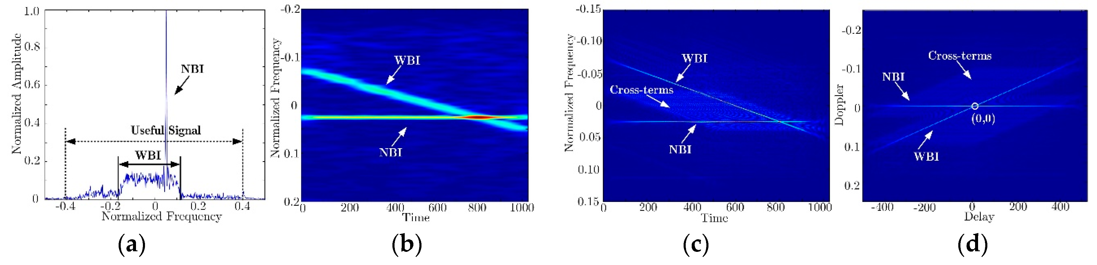
Figure 1a shows the frequency spectrum of received signal with NBI and LFM-WBI. It is obvious that NBI is easily captured according to its amplitude changes in frequency domain, while the spectrum of LFM-WBI distributes along the whole frequency band, which increases difficulties in interference identification and suppression. For STFT, the interferences are concentrated along the straight lines in the TF plane, which occupies much smaller frequency bins at each time slice than in the frequency domain, as illustrated in Figure 1b. For WD, it has a good energy concentration property for LFM signals. However, for multiple components, an unwanted cross-terms problem may severely impede auto-terms identification, as shown in Figure 1c. Although the cross-terms also occur in the AF plane, AF has a useful property that the auto-terms pass through the origin of AF plane and the cross-terms are away from it, as illustrated in Figure 1d. Based on this property, the auto-terms of interference are easily identified. Thus, an interference suppression algorithm in AF plane is proposed in the following.
3. Interference Suppression Algorithm Using AF-CAF-IDA
In this section, AF-CAF-IDA based interference suppression is introduced. This algorithm consists of three stages: (1) SSM from AF-CAF; (2) binary mask construction for interference identification and extraction; and (3) IDA using SSM and mask construction. In the following, interference suppression including SSM and binary mask construction is discussed in details.
3.1. SSM from AF-CAF for Mono-Component Signal
Assume a discrete mono-component signal with N samples in length, and its vector form is denoted as . To obtain its AF, symmetric instantaneous autocorrelation function (SIAF) of is calculated first, which can be expressed as
where is the conjugate operator. Matrix form of is written as
For the convenience of description, Figure 2 gives the structure of with N being 5. The AF of can be obtained by calculating the one-dimensional (1-D) inverse Fast Fourier Transform (IFFT) of each row of , defined by
According to above operations, the received echo can be transformed into AF plane. If is known, can be reconstructed by following steps.
First, calculate matrix by 1-D Fast Fourier Transform (FFT), which is expressed as
Here, we consider another matrix with its elements defined by , where . If matrix is given, the original signal can be obtained by eigenvalue decomposition (EVD), expressed as [42]
where and represent the eigenvalue and corresponding eigenvectors, respectively. The matrix of has only one nonzero eigenvalue, with which the original signal can be recovered as follows:
where is the constant phase.
The above signal synthesis method is under the assumption that is known. However, according to Equation (7), only matrix can be obtained from the AF. Fortunately, compared with , the relationship between and can be summarized as follows: the elements in the m-th row of are located at 2m-th auxiliary diagonal of , as shown in Figure 2. Based on this property, a new matrix can be constructed by matrix rearrangement, defined by
From Equation (10), it is clear that half of elements are zeros. To obtain the remaining elements in , CAF transform is introduced. Consider another discrete signal , the symmetric instantaneous cross-correlation function (SICF) between and is calculated by
Its matrix form can be written as
From Equation (12), the CAF of and can be obtained by calculating the 1-D IFFT of each row of , defined by
Similarly, if is given, can be calculated by 1-D FFT, depicted as
To obtain the remaining elements in the (2m − 1)-th auxiliary diagonal of , we let , then can be reconstructed, as shown in Figure 2. Compared with , we can draw another conclusion that the elements in the m-th row of are located at (2m − 1)-th auxiliary diagonal of upper triangular matrix in . The elements in the (2m − 1)-th auxiliary diagonal of lower triangular matrix in can be easily obtained, due to its characteristic of Hermitian matrix (i.e., ). According to this property, another new matrix can be constructed by matrix rearrangement, defined by
Therefore, can be obtained by combining with . Then, the original signal can be reconstructed by EVD.
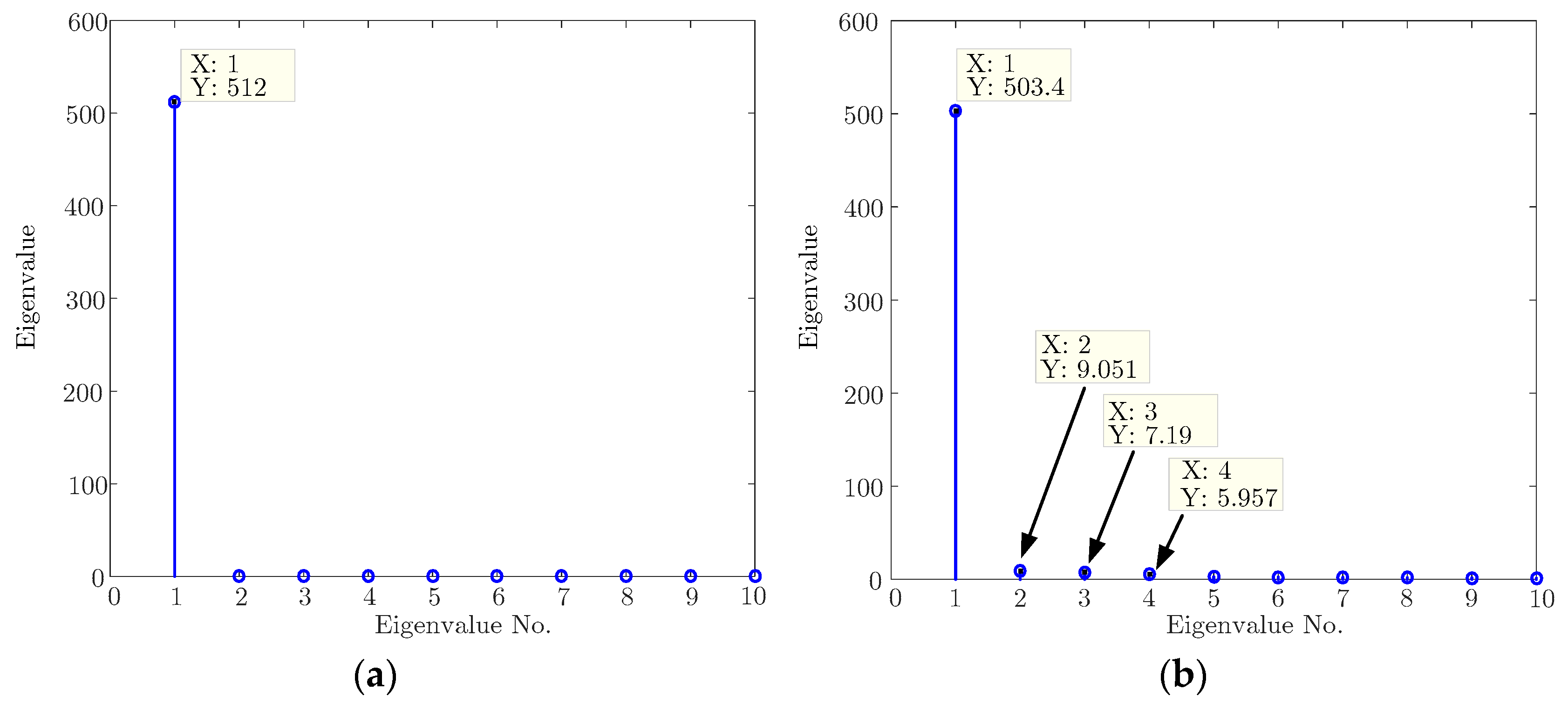
Compared with traditional SSM from WD, the major difference is the construction of matrix. In the traditional SSM from WD, an interpolation to WD is necessary, and all elements in the matrix R need to be calculated by discrete Fourier transform (DFT) one by one. In the SSM from AF-CAF, the matrix of R can be obtained by rearranging the matrix from the AF and CAF, and the elements in R can be calculated by FFT. Thus, it is time saving. Here, we take a signal with 512 samples in length as an example to check calculation time and signal energy loss. Results show that the calculation time of traditional synthesis method is 3.5 times of that of SSM from AF-CAF. The eigenvalues obtained by SSM from AF-CAF are shown in Figure 3a. There is only one nonzero eigenvalue with its energy being 512. Compared with traditional signal synthesis method, there are several nonzero eigenvalues, and the largest one is 503.4, as illustrated in Figure 3b. The signal energy loss is caused by the interpolation to the WD. Therefore, SSM from AF-CAF is more accurate.
3.2. SSM from AF-CAF for Multi-Component Signal
In this section, the SSM from AF-CAF for multi-component signal is presented. Consider a multi-component signal
where subscript i denotes the i-th component of signal. The SIAF of can be written as
Substituting Equation (17) into Equation (6) yields
where and represent the auto-terms and cross-terms, respectively. Suppose that the cross-terms have been eliminated completely, the masked AF (MAF) is equal to the sum of AFs of individual components, which can be expressed as follows:
Substituting Equation (19) into Equation (7), we have
From Equation (20), it is obvious that inverse MAF equals to the sum of the inverse AFs of individual components. After that, the matrix rearrangement is applied to reconstruct the matrix .
Similarly, the SICF of and () can be expressed as
The CAF of and can be given by
where and represent the auto-terms and cross-terms, respectively. Assume that the cross-terms in CAF domain are removed clearly; the mask CAF (MCAF) also equals the sum of the CAFs of individual components, expressed as
The inverse CAF of Equation (23) is given by
It can be seen that inverse MCAF equals the sum of the inverse CAFs of individual components and the matrix can be obtained by matrix rearrangement. After combining and , can be rewritten as follows:
After EVD, the multi-component signal can be synthesized by
3.3. Binary Mask Construction for Signal Extraction and Cross-Terms Suppression
The analysis above is based on the assumption that the cross-terms are removed clearly, otherwise Equation (26) would no longer hold. In this section, the mask algorithm is presented to suppress cross-terms. In the AF and CAF domain, the auto-terms of multi-LFM component signal have two properties:
Property 1.
Auto-terms have line-like features in the AF and CAF domains.
Property 2.
Auto-terms pass through the origins of the AF and CAF domains, while the cross-terms are away from the origins.
For detailed discussion and proof, please refer to Appendix A.
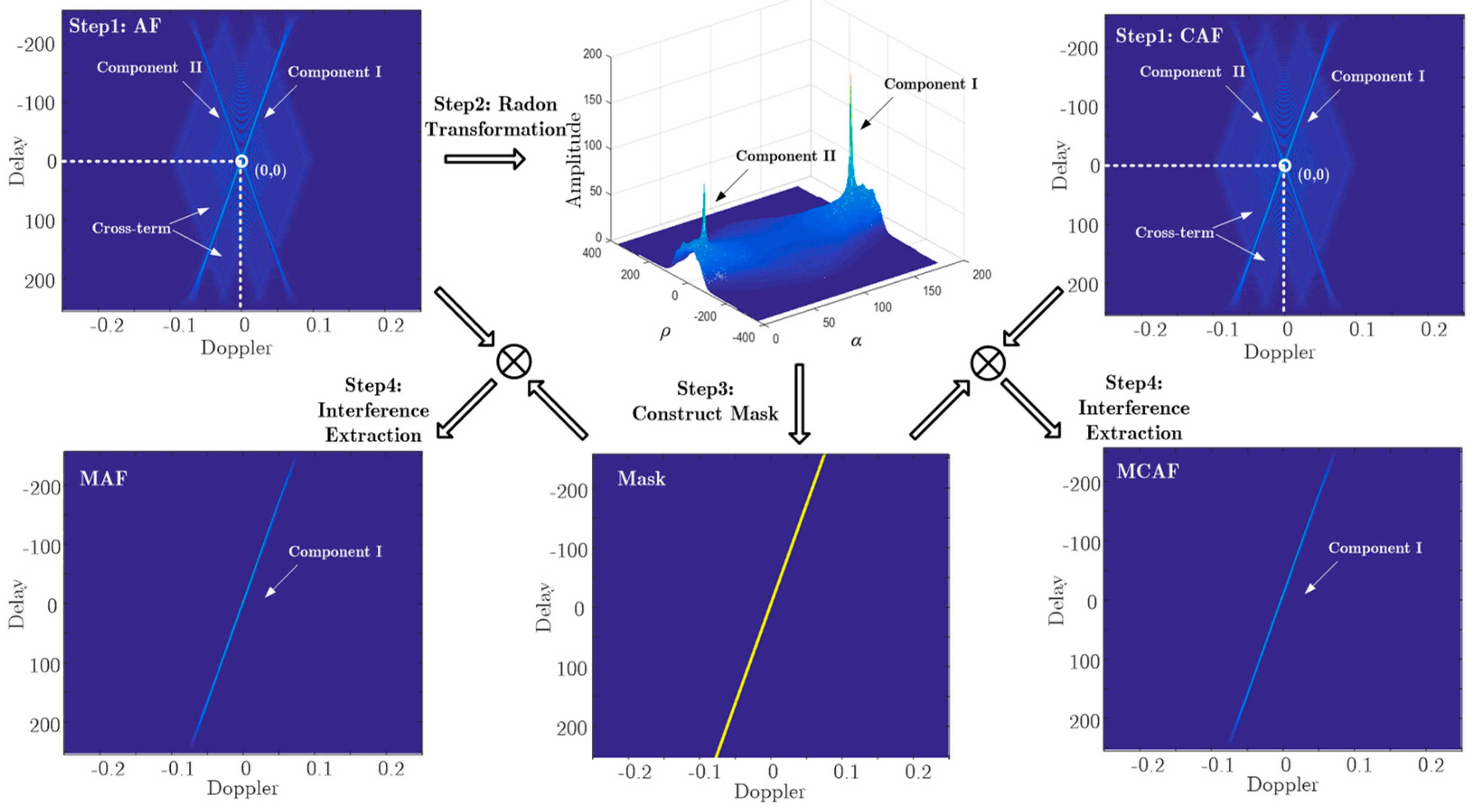
According to these two properties, an interference identification and cross-term suppression algorithm is proposed. Based on Property 1, Radon transform (RT) is utilized to integrate the auto-terms along the straight line and the integral value exhibits a distinct peak in the Radon AF (RAF) plane. The RT is defined by
where is the delta function, and and represent the polar distance and polar angle, respectively. Based on Property 2, auto-terms in the RAF plane are certainly located at zeros-polar distance slice (i.e., ). According to these properties, auto-terms of interference can be integrated and identified at slice in polar distance and polar angle () domain, as shown in Figure 4. If the amplitude at slice jumps with peaks much larger than the mean value, then one can conclude that the data may be contaminated by interferences. In addition, the inverse RT is utilized to extract the interference and suppress the cross-terms.
The processes of mask algorithm in the AF and CAF can be depicted as follows:
- (1)
- Calculate the AF () and CAF () of the received signals, respectively.
- (2)
- Determine the RAF (), and then perform a 1-D search at slice to identify the interference and record the maximum peak position . After that, compute the inverse RT with and , denoted as .
- (3)
- Compare the elements of with zero, and then binary mask can be expressed as follows:
- (4)
- Extract the interference in the AF and CAF plane as follows:
For simplicity, a flowchart of interference identification and extraction using mask algorithm is shown in Figure 4. After interference, identification and extraction, the interference can be recovered by SSM from MAF and MCAF.
3.4. SAR Imaging with AF-CAF-IDA Based Interference Suppression
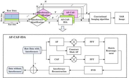
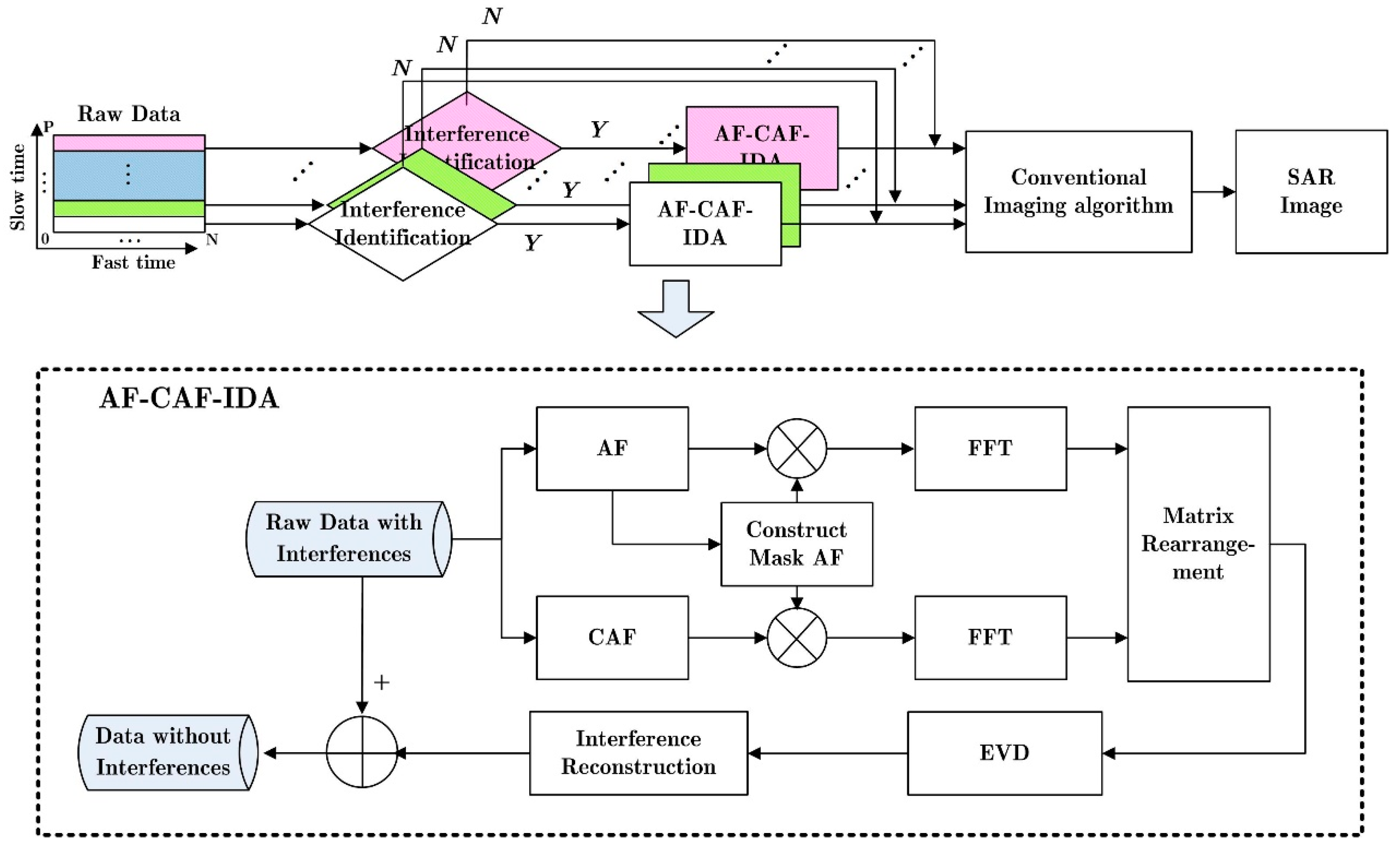
According to the aforementioned analysis, AF-CAF-IDA is proposed to identify and suppress the interference. For simplicity, the flowchart of SAR image formation from raw data contaminated by interferences using the proposed scheme is shown in Figure 5. The detailed procedures can be summarized as the following steps:
Step 1: Extract the p-th azimuth sample data , where , , N and P represent the total samples in fast time and slow time, respectively.
Step 2: Transform into the RAF domain to detect whether the interference exists. If interference exists, AF-CAF-IDM is utilized to suppress interference, as shown in dashed area of Figure 4; otherwise. go to Step 3. The AF-CAF-IDM consists of following steps:
- (1)
- Calculate the MAF and MCAF of received signal according to mask algorithm.
- (2)
- Rearrange the IFFT of MAF and MCAF and recovery the signal via EVD, and then estimate the parameter by solving the following equation:
- (3)
- Subtract the synthesized component from the received signal and iterate above steps until all interferences in the p-th azimuth sample data are suppressed.
Step 3: Let ; if p is less than or equal to P, iterate above steps to ensure interferences at each azimuth gate are completely eliminated. Finally, a well-focused SAR image is obtained by the conventional radar imaging algorithm.
To demonstrate the validity of AF-CAF-IDA, a chirp signal (i.e., useful signal) with NBI and LFM-WBI is generated. The signal can be modeled by
where
where , and represent the chirp signal, NBI and LFM-WBI, respectively. is additive Gaussian noise with the signal-to-noise-ratio (SNR) being 5 dB. Figure 6a shows the frequency spectrum of . In the presence of the interferences, the chirp signal is seriously contaminated by NBI and LFM-WBI. Figure 6b shows the WD of , where NBI and LFM-WBI are well concentrated in TF plane with cross-terms. However, it is difficult to distinguish the auto-terms and cross-terms in the WD domain. Figure 6c gives the AF of the received signal. It is obvious that the auto-terms of chirp signal, NBI and LFM-WBI pass through the origin of the AF plane, and cross-terms are away from it. Furthermore, the auto-terms of chirp signal is highly overlapped with that of LFM-WBI, since they have the same chirp rates. Therefore, two cases should be considered in this example.
Case (1): Mono-component signal synthesis. After conducting the mask algorithm, the greatest signal (i.e., NBI) is extracted, as shown in Figure 6d. By performing the EVD, only one large eigenvalue corresponding to the NBI is obtained, as illustrated in Figure 6e. In Figure 6f, a comparison between the reconstructed signal and the original NBI is presented, which implies that the synthesized signal is in good agreement with the original signal. It is obvious that the NBI is eliminated cleanly after subtracting reconstructed signal from the original signal, as shown in Figure 6g.
Case (2): Multi-component signal synthesis. After performing the mask algorithm, the MAF of the rest signal is equal to the sum AFs of chirp signal and LFM-WBI, as illustrated in Figure 6h. In Figure 6i, there are two large eigenvalues corresponding to the chirp signal and LFM-WBI, respectively, which is consistent with Equation (25). Figure 6j gives the comparison of the real part between the synthesized LFM-WBI and original component. It is clear that the synthesized component fits well with the original one. After subtracting the LFM-WBI from the rest signal, the desired chirp signal is obtained. Figure 6k,l presents the WD of the chirp signal and its real part, respectively. From this example, we can conclude that AF-CAF-IDA is effective for interference suppression with only a small loss of signal.
4. Experimental Analysis
The above sections have addressed interference suppression based on AF-CAF-IDA theory. In this section, we demonstrate the effectiveness of the interference suppression algorithm by dealing with SAR data.
4.1. Comparison between Interference Suppression Algorithms
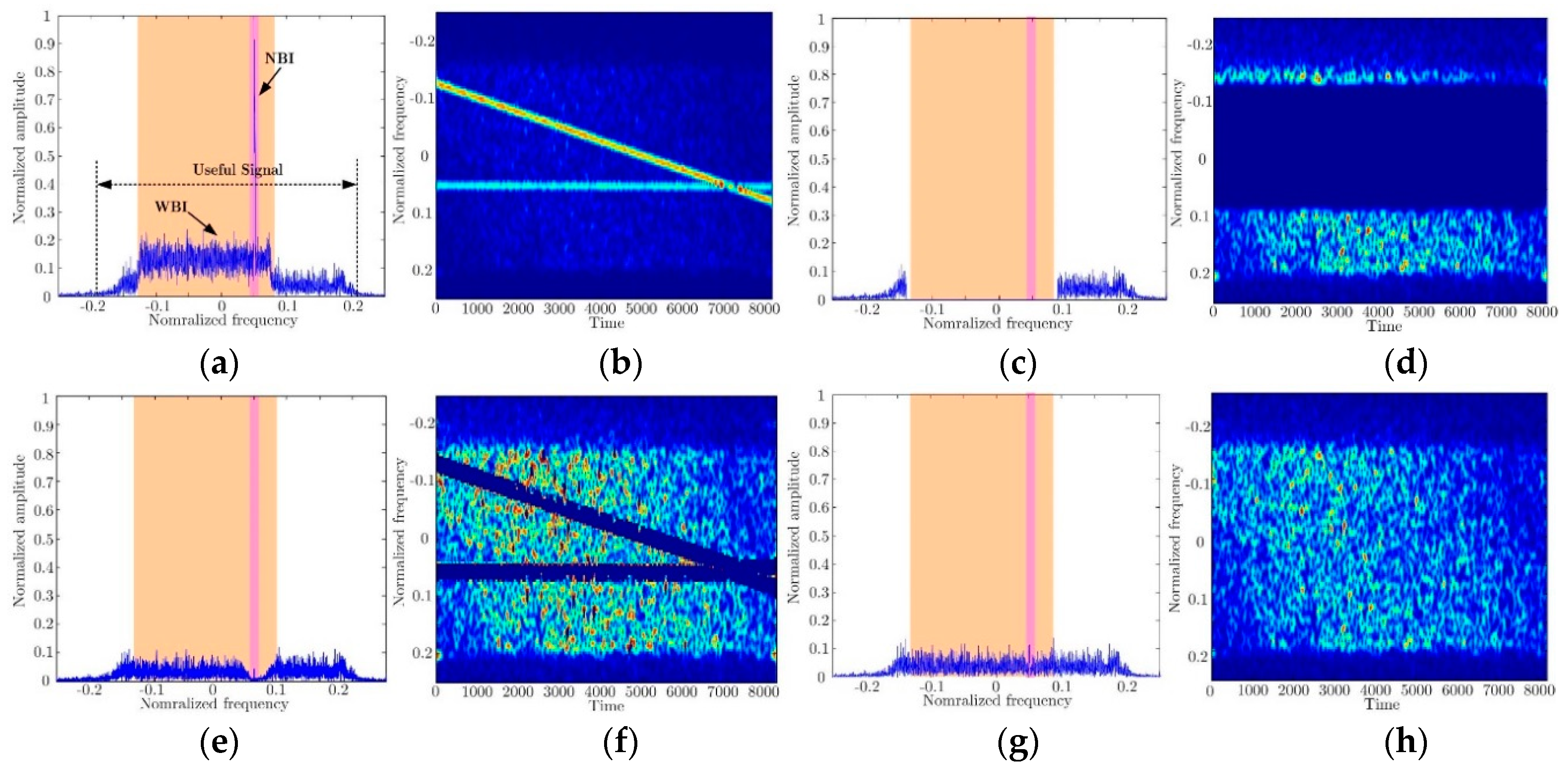
In this part, comparisons of the frequency-notch filtering, TF filtering and AF-CAF-IDA are provided. The simulated NBI and LFM-WBI are added to the real SAR data to verify the validity of AF-CAF-IDA. After range compression, Figure 7a,b presents the frequency spectrum and TF spectrogram of SAR echo with interferences, respectively. It is clear that the frequency spectrum of LFM-WBI occupies many frequency bins. If the frequency-domain notch filter is adopted, the useful information, which is overlapped with the LFM-WBI in the frequency spectrum, are also removed simultaneously, as shown in Figure 7a,d. The NBI and LFM-WBI are concentrated along the straight lines in the TF plane with only a fraction of frequency bins occupied at each time slices, as shown in Figure 7b. The filtering in the TF plane can suppress the interferences with smaller loss of the useful signal than frequency notch does, and its frequency spectrum and TF spectrogram are given in Figure 7e,f. Figure 7g,h illustrates the results of AF-CAF-IDA based interference suppression algorithm. In this figure, it is observed that interferences are eliminated completely while the useful signal is preserved well. To make a quantitative evaluation of the proposed algorithm, signal distortion ration (SDR) is introduced, which is defined by [36]
where represents the signal after interference suppression and denotes the original signal without interference. The SDR of these three algorithms are calculated and the results are listed in Table 2. In this table, it is noted that the signal losses of frequency-notch filtering and TF filtering are greater than that of the proposed algorithm, which implies that AF-CAF-IDA can not only suppresses the interference but also preserve the signal energy as much as possible.
4.2. Results of Measured Data
In this section, measured SAR data contaminated by serious interference are utilized. To present the image quality improvement of proposed algorithm, two metrics of SNR and contrast in the image domain [36] are introduced in the following discussion. The SNR is defined as
where represents the i-th prominent scatterer and denotes the j-th pixel of the surrounding region. and denote the number of prominent scatterer pixels and noise pixels, respectively. A greater SNR results in a better focused image. Another metric is image contrast. For a P × N SAR image (P is the number of pixels in range, and N is the number in the azimuth), its contrast can be defined as
where represents the (p-th, n-th) pixel in the SAR image; denotes the mean value of the signal. From Equation (35), the greater the contrast D is, the better the image quality well be.
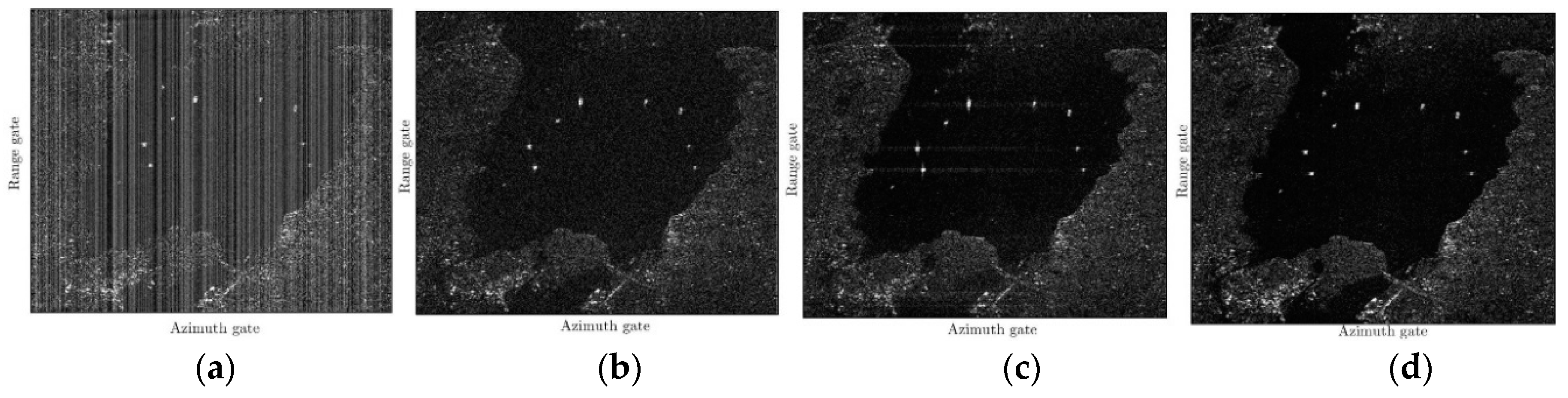
(1) Result of NBI Suppression: Figure 8a presents the SAR image with NBI, where the bright lines overshadow the important features, such as the ships and fields. Figure 8b presents the SAR image after frequency-domain notch filtering. Although the majority of interference energy in frequency bins has been suppressed, the useful information, which is located in the same bins, is also removed clearly. Due to significant portion loss of useful signal, the SNR of the imagery may degrade. Figure 8c shows the imaging result after NBI suppression using TF filtering. Compared with Figure 8b, only a small fractional of useful signal is lost and image contours have more clarity. However, it is clearly seen that the targets are defocused. Figure 8d presents the SAR image after AF-CAF-IDA. It is observed that the image is well focused and bright lines have been suppressed efficiently. In addition, the SNR and contrast D for three interference suppression algorithms are calculated. In Table 3, AF-CAF-IDA is with greater SNR and contrast than TF filter and notch filter methods, which not only suppresses the NBI but also preserves the useful information as much as possible.
(2) Result of WBI Suppression: Figure 9a shows the image with LFM-WBI, where most portion of the scene in the image is covered due to existence of LFM-WBI. Figure 9b,c presents the imaging result after frequency-domain notch filtering and TF filtering, respectively. Because the majority of useful signal is interfered and filtered, the image is contaminated by noise and we can only see blurred image contours. Figure 9d shows the imaging result after AF-CAF-IDA. A clear image with village, mountain, river and fields is presented. Furthermore, the results of SNR and contrast for these three interference suppression algorithms are listed in Table 4, indicating the advantages of the proposed algorithm over the others. To sum up, AF-CAF-IDA based interference algorithm can effectively suppress LFM-WBI with the useful signal being kept well.
5. Conclusions
In this paper, the Delay-Doppler distributions of time-varying SAR interferences (i.e., NBI and LFM-WBI) are analyzed via AF and CAF for the first time. By making full use of the properties in Delay-Doppler domain, a nonparametric interference suppression method based on the Delay-Doppler iterative decomposition algorithm is proposed. This algorithm has three advantages: (1) Compared with STFT, time-varying interference analysis in the Delay-Doppler domain has an excellent energy concentration property. (2) Compared with WD, AF has a unique property that the auto-terms pass through the origin of Delay-Doppler domain while cross-terms are away from it. Therefore, masking in the AF can solve the cross-terms identifiability problem and are very suitable for interference identification and extraction. (3) Since the matrix rearrangement and FFT are utilized, SSM from AF and CAF is more accurate and faster than the traditional SSM from WD. Thanks to these advantages, the proposed algorithm not only suppresses interference but also preserves the useful information as much as possible. The performance (such as SDR, SNR and Contrast) analyses of the simulated data and measured data demonstrate that the proposed algorithm outperforms the notch filtering method and the TF filtering method.
Author Contributions
Conceptualization, J.S.; Funding acquisition, J.S., M.T., J.X. and L.W.; Investigation, J.S. and M.T.; Methodology, J.S.; Supervision, H.T. and L.W.; Validation, H.T. and L.W.; Writing—original draft, J.S., M.T. and Y.W.; and Writing—review and editing, J.S., H.T., M.T., J.X., Y.W. and L.W.
Funding
This research was funded by National Nature Science Foundation of China (NSFC) under Grants 61701414, 61801390, 61601372 and 61601373. This work was also supported by Science and Technology Fund Project, Postdoctoral Innovation Talent Support Program under Grant BX201700199 and China Postdoctoral Science Foundation under Grant 2018M631123 and 2017M623240.
Acknowledgments
The authors would like to thank the reviewers for their very helpful and useful suggestions, which have considerably improved the quality of the manuscript.
Conflicts of Interest
The authors declare no conflict of interest.
Appendix A
To demonstrate two properties of the AF and CAF domains, we take a chirp signal (useful signal) contaminated by an LFM-WBI for example to discuss auto-terms and cross-terms of multi-component signal in AF plane, defined by
The SIAF of Equation (A1) can be written as follows:
where and represent the instantaneous autocorrelation of useful signal and LFM-WBI, respectively; denotes the cross correlation between useful signal and LFM-WBI; and indicates the real part operator. Therefore, the AF of mixed signal can be obtained by
where , and represent the auto-terms of useful signal and LFM-WBI, respectively, and represents the cross-terms. According to Equation (A3), we can conclude that the auto-terms of multi-component LFM signals in the AF plane have two properties: (Property 1) the auto-terms have line-like feature in the AF plane; and (Property 2) the auto-terms pass through the origin of the AF plane while the cross-terms are away from it.
The SICF of and can be expressed as
where represents the instantaneous cross-correlation between and ; , , and are defined in the same way as ; and , , , are given as
Thus, the CAF of and can be expressed as
where and represent the auto-terms of useful signal and LFM-WBI, respectively; and and are the cross-terms. Comparing Equations (A3) and (A6), the auto-terms have line-like feature (Property 1), while they do not pass through the origin of CAF plane. Fortunately, the chirp rate of LFM signal is usually within [−1/N, 1/N] to avoid the Doppler aliasing, which implies that the distances from auto-terms to origin are smaller than half of the Doppler bin. Thus, auto-terms in the CAF plane can be approximately considered as passing through the origin (Property 2).
References
- Huang, P.; Liao, G.; Yang, Z.; Xia, X.G.; Ma, J.T.; Ma, J. Long-time coherent integration for weak maneuvering target detection and high-order motion parameter estimation based on keystone transform. IEEE Trans. Signal Process. 2016, 64, 4013–4026. [Google Scholar] [CrossRef]
- Zhang, X.; Liao, G.; Zhu, S.; Zeng, C.; Shu, Y. Geometry-information-aided efficient radial velocity estimation for moving target imaging and location based on radon transform. IEEE Trans. Geosci. Remote Sens. 2015, 53, 1105–1117. [Google Scholar] [CrossRef]
- Natsuaki, R.; Motohka, T.; Watanabe, M.; Shimada, M.; Suzuki, S. An autocorrelation-based radio frequency interference detection and removal method in azimuth-frequency domain for SAR Image. IEEE J. Sel. Top. Appl. Earth Obs. Remote Sens. 2017, 10, 5736–5751. [Google Scholar] [CrossRef]
- Wang, W.-Q.; Shao, H. Radar-to-radar interference suppression for distributed radar sensor networks. Remote Sens. 2014, 6, 740–755. [Google Scholar] [CrossRef]
- Luo, X.; Ulander, L.M.; Askne, J.; Smith, G.; Frolind, P.O. RFI suppression in ultra-wideband SAR systems using LMS filters in frequency domain. Electron. Lett. 2001, 37, 241–243. [Google Scholar] [CrossRef]
- Miller, T.; Potter, L.; Mccorkle, J. RFI suppression for ultra wideband radar. IEEE Trans. Aerospace Electron. Syst. 1997, 33, 1142–1156. [Google Scholar] [CrossRef]
- Load, R.T.; Inggs, M.R. Efficient RFI suppression in SAR using LMS adaptive filter integrated with rang/Doppler algorithm. Electron. Lett. 1999, 35, 629–630. [Google Scholar] [CrossRef]
- Won, J.H.; Pany, T.; Eissfeller, B. Iterative Maximum Likelihood Estimators for High-Dynamic GNSS Signal Tracking. IEEE Trans. Aerosp. Electron. Syst. 2012, 48, 2875–2893. [Google Scholar] [CrossRef]
- Smith, T.L.; Hill, R.D.; Hayward, S.D.; Yates, G.; Blake, A. Filtering approaches for interference suppression in low-frequency SAR. IEE Proc. Radar Sonar Navig. 2006, 153, 338–344. [Google Scholar] [CrossRef]
- Jayant, H.K.; Rana, K.P.; Kumar, V.; Nair, S.S.; Mishra, P. Efficient IIR notch filter design using Minimax optimization for 50Hz noise suppression in ECG. In Proceedings of the 2015 IEEE International Conference on Signal Processing, Computing and Control, Waknaghat, India, 24–26 September 2015; pp. 290–295. [Google Scholar] [CrossRef]
- Mishra, S.; Das, D.; Kumar, R.; Sumathi, P. A Power-Line Interference Canceler Based on Sliding DFT Phase Locking Scheme for ECG Signals. IEEE Trans. Instrum. Meas. 2014, 64, 132–142. [Google Scholar] [CrossRef]
- Ren, A.; Du, Z.; Li, J.; Hu, F.; Yang, X.; Abbas, H. Adaptive Interference Cancellation of ECG Signals. Sensors 2017, 17, 942. [Google Scholar] [CrossRef] [PubMed]
- Thakor, N.V.; Zhu, Y.S. Applications of adaptive filtering to ECG analysis: Noise cancellation and arrhythmia detection. IEEE Trans. Biomed. Eng. 1991, 38, 785–794. [Google Scholar] [CrossRef] [PubMed]
- Zhou, F.; Wu, R.; Xing, M.; Bao, Z. Eigen subspace-based filtering with application in narrowband interference suppression for SAR. IEEE Geosci. Remote Sens. Lett. 2007, 4, 75–79. [Google Scholar] [CrossRef]
- Zhou, F.; Tao, M.; Bai, X.; Liu, J. Narrow-Band Interference Suppression for SAR Based on Independent Component Analysis. IEEE Trans. Geosci. Remote Sens. 2013, 51, 4952–4960. [Google Scholar] [CrossRef]
- Tao, M.; Zhou, F.; Liu, Y.; Zhang, Z. Tensorial Independent Component Analysis-Based Feature Extraction for Polarimetric SAR Data Classification. IEEE Trans. Geosci. Remote Sens. 2015, 53, 2481–2495. [Google Scholar] [CrossRef]
- Tao, M.; Zhou, F.; Liu, J.; Liu, Y.; Zhang, Z.; Bao, Z. Narrow-Band Interference Mitigation for SAR Using Independent Subspace Analysis. IEEE Trans. Geosci. Remote Sens. 2014, 52, 5289–5301. [Google Scholar] [CrossRef]
- Zhou, F.; Xing, M.; Bai, X.; Sun, G.; Bao, Z. Narrowband interference suppression for SAR based on complex empirical mode decomposition. IEEE Geosci. Remote Sens. Lett. 2009, 6, 423–427. [Google Scholar] [CrossRef]
- Huang, Y.; Liao, G.; Li, J.; Xu, J. Narrowband RFI suppression for SAR system via fast implementation of joint sparsity and low-rank property. IEEE Trans. Geosci. Remote Sens. 2018, 56, 2748–2761. [Google Scholar] [CrossRef]
- Darsena, D.; Gelli, G.; Paura, L.; Verde, F. NBI-resistant zero-forcing equalizers for OFDM systems. IEEE Commun. Lett. 2005, 9, 744–746. [Google Scholar] [CrossRef]
- Redfern, A.J. Receiver window design for multicarrier communication systems. IEEE J. Sel. Areas Commun. 2002, 20, 1029–1036. [Google Scholar] [CrossRef]
- Ding, M.; Redfern, A.J.; Evans, B.L. A dual-path TEQ structure for DMT-ADSL systems. In Proceedings of the 2002 IEEE International Conference on Acoustics, Speech, and Signal Processing, Orlando, FL, USA, 2002; pp. III-2573–III-2576. [Google Scholar] [CrossRef]
- Ma, X.Y.; Qin, J.M.; He, Z.H.; Yang, J.; Lu, Q.H. Three-channel cancellation of SAR blanketing jamming suppression. Acta Electron. Sin. 2007, 35, 1015–1020. [Google Scholar]
- Wang, H.L. Comparative analysis of adaptive beamforming algorithms for satellite multiple-beam antennas. Acta Electron. Sin. 2001, 29, 358–360. [Google Scholar]
- Liu, H.; Li, D.; Zhou, Y.; Truong, T.K. Simultaneous Radio Frequency and Wideband Interference Suppression in SAR Signals via Sparsity Exploitation in Time-Frequency Domain. IEEE Trans. Geosci. Remote Sens. 2018, 1–14. [Google Scholar] [CrossRef]
- Elgamel, S.A.; Soraghan, J.J. Using EMD-FrFT filtering to mitigate very high power interference in chirp tracking radars. IEEE Signal Process. Lett. 2011, 18, 263–266. [Google Scholar] [CrossRef] [Green Version]
- Peleg, S.; Friedlander, B. The discrete polynomial-phase transform. IEEE Trans. Signal Process. 1995, 43, 1901–1914. [Google Scholar] [CrossRef]
- Porat, B.; Friedlander, B. Asymptotic statistical analysis of the high-order ambiguity function for parameter estimation of polynomial-phase signals. IEEE Trans. Inf. Theory 1996, 42, 995–1001. [Google Scholar] [CrossRef]
- Djukanovic, S.; Popovic, V. A Parametric Method for Multicomponent Interference Suppression in Noise Radars. IEEE Trans. Aerospace Electron. Syst. 2012, 48, 2730–2738. [Google Scholar] [CrossRef]
- Barbarossa, S. Analysis of multicomponent LFM signals by a combined Wigner-Hough transform. IEEE Trans. Signal Process. 1995, 43, 1511–1515. [Google Scholar] [CrossRef]
- Wood, J.C.; Barry, D.T. Radon transformation of time-frequency distributions for analysis of multicomponent signals. IEEE Trans. Signal Process. 1994, 42, 3166–3177. [Google Scholar] [CrossRef]
- Wang, M.; Chan, A.K.; Chui, C.K. Linear frequency-modulated signal detection using Radon-ambiguity transform. IEEE Trans. Signal Process. 1998, 46, 571–586. [Google Scholar] [CrossRef]
- Su, J.; Tao, H.H.; Rao, X.; Xie, J.; Guo, X.L. Coherently integrated cubic phase function for multiple LFM signals analysis. Electron. Lett. 2015, 51, 411–413. [Google Scholar] [CrossRef]
- Sergio, B.; Anna, S. Adaptive time-varying cancellation of wideband interference in spread-spectrum communications based on time-frequency distributions. IEEE Trans. Signal Process. 1999, 47, 957–965. [Google Scholar] [CrossRef]
- Li, Y.; Ye, L.; Sha, X. Time-Frequency Energy Sensing of Communication Signals and Its Application in Co-Channel Interference Suppression. Sensors 2018, 18, 2378. [Google Scholar] [CrossRef] [PubMed]
- Zhang, S.; Xing, M.; Guo, R.; Zhang, L.; Bao, Z. Interference Suppression Algorithm for SAR based on time–frequency transform. IEEE Trans. Geosci. Remote Sens. 2011, 49, 3765–3779. [Google Scholar] [CrossRef]
- Zhao, T.; Zhang, Y.; Yang, L.; Dong, Z.; Liang, D. The RFI suppression method based on STFT applied to SAR. Prog. Electromagn. Res. M 2013, 31, 171–188. [Google Scholar] [CrossRef]
- Yang, Z.; Du, W.; Liu, Z.; Liao, G. WBI Suppression for SAR Using Iterative Adaptive Method. IEEE J. Sel. Top. Appl. Earth Obs. Remote Sens. 2016, 9, 1008–1014. [Google Scholar] [CrossRef]
- Tao, M.; Zhou, F.; Zhang, Z. Wideband Interference Mitigation in High-Resolution Airborne Synthetic Aperture Radar Data. IEEE Trans. Geosci. Remote Sens. 2015, 54, 74–87. [Google Scholar] [CrossRef]
- Lao, G.; Yin, C.; Ye, W.; Sun, Y.; Li, G. A Frequency Domain Extraction Based Adaptive Joint Time Frequency Decomposition Method of the Maneuvering Target Radar Echo. Remote Sens. 2018, 10, 266. [Google Scholar] [CrossRef]
- Su, J.; Tao, H.; Tao, M.; Wang, L.; Xie, J. Narrow-Band Interference Suppression via RPCA-Based Signal Separation in Time–Frequency Domain. IEEE J. Sel. Top. Appl. Earth Obs. Remote Sens. 2017, 10, 5016–5025. [Google Scholar] [CrossRef]
- Boudreaux-Bartels, G.; Parks, W. Time-varying filtering and signal estimation using Wigner distribution synthesis techniques. IEEE Trans. Acoust. Speech Signal Process. 1986, 34, 442–451. [Google Scholar] [CrossRef]
- Zuo, L.; Li, M.; Zhang, X.; Wang, Y.; Wu, Y. An Efficient Method for Detecting Slow-Moving Weak Targets in Sea Clutter Based on Time–Frequency Iteration Decomposition. IEEE Trans. Geosci. Remote Sens. 2013, 51, 3659–3672. [Google Scholar] [CrossRef]
- Li, D.; Liu, H.; Yang, L. Efficient time-varying interference suppression method for synthetic aperture radar imaging based on time-frequency reconstruction and mask technique. IET Radar Sonar Navig. 2015, 9, 827–834. [Google Scholar] [CrossRef]
- Sharif, M.R.; Abeysekera, S.S. Efficient wideband signal parameter estimation using a radon-ambiguity transform slice. IEEE Trans. Aerospace Electron. Syst. 2007, 43, 673–688. [Google Scholar] [CrossRef]
Figure 1.
The (a) frequency spectrum; (b) STFT; (c) WD; and (d) AF of NBI and LFM-WBI.

Figure 2.
Matrix rearrangement from AF and CAF.
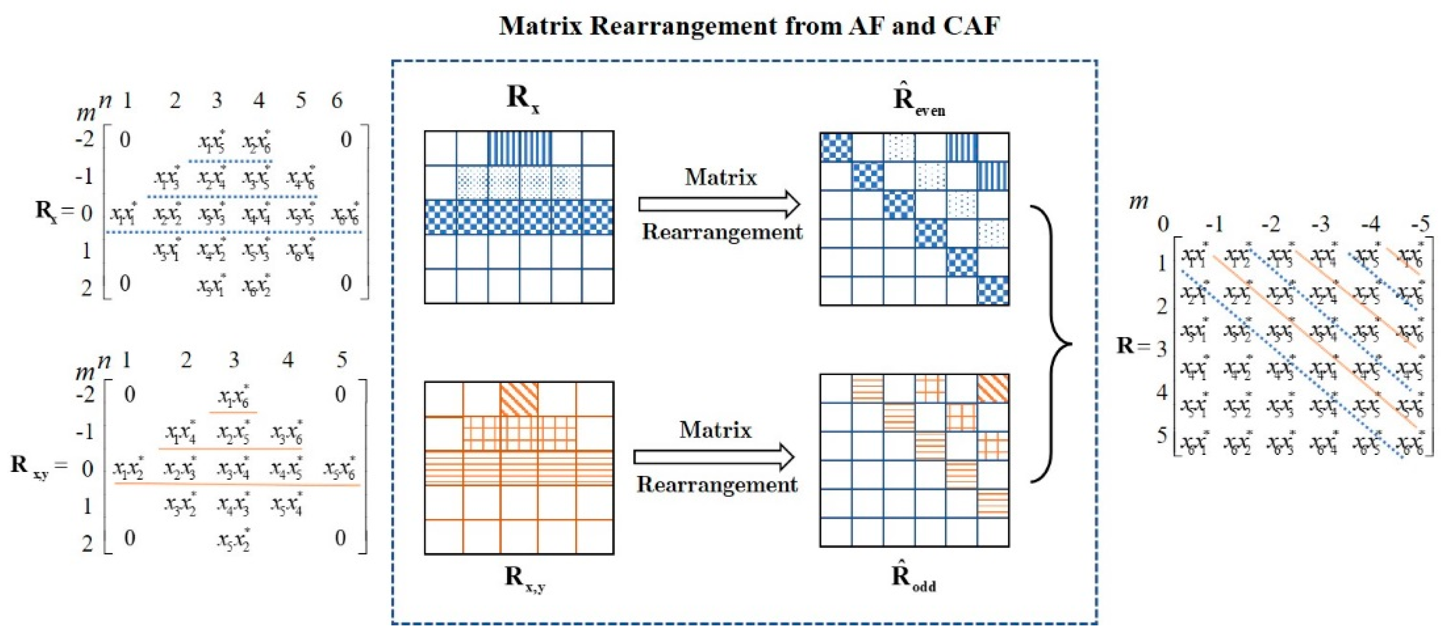
Figure 3.
Eigenvalues by the SSM from AF-CAF and traditional SSM from WD method: (a) SSM from AF-CAF; and (b) traditional SSM from WD.
Figure 3.
Eigenvalues by the SSM from AF-CAF and traditional SSM from WD method: (a) SSM from AF-CAF; and (b) traditional SSM from WD.

Figure 4.
The flowchart of interference identification and extraction using mask algorithm.

Figure 5.
Flowchart of AF-CAF-IDA based Interference Suppression.

Figure 6.
Interference suppression based on AF-CAF-IDA: (a) frequency spectrum of the original signal; (b) WD of the original signal. (c) AF of the original signal; (d) NBI extraction from the original signal; (e) eigenvalues obtained from masked signal (NBI); (f) real part of the reconstructed NBI; (g) AF of the rest signal; (h) MAF of the rest signal; (i) eigenvalues obtained from masked signal (LFM-WBI and chirp signal); (j) real part of the reconstructed LFM-WBI; (k) WD of the chirp signal; and (l) real part of the chirp signal.

Figure 7.
Comparison between interference suppression methods: (a) frequency spectrum of signal with interferences; (b) spectrogram of signal with interferences; (c) frequency spectrum of signal after frequency-domain notch filtering; (d) spectrogram of signal after frequency-domain notch filtering; (e) frequency spectrum of signal after TF filtering; (f) spectrogram of signal after TF filtering; (g) frequency spectrum of signal with LFM-WBI after AF-CAF-IDA; and (h) spectrogram of signal with LFM-WBI after AF-CAF-IDA.

Figure 8.
Imaging results of NBI suppression: (a) image of raw data; (b) image after frequency-domain notched filtering; (c) image using the TF filtering; and (d) image using AF-CAF-IDA.
Figure 8.
Imaging results of NBI suppression: (a) image of raw data; (b) image after frequency-domain notched filtering; (c) image using the TF filtering; and (d) image using AF-CAF-IDA.

Figure 9.
Imaging results of WBI suppression: (a) image of raw data; (b) image after frequency-domain notched filtering; (c) image using the TF filtering; and (d) image using AF-CAF-IDA.
Figure 9.
Imaging results of WBI suppression: (a) image of raw data; (b) image after frequency-domain notched filtering; (c) image using the TF filtering; and (d) image using AF-CAF-IDA.


Table 1.
Main abbreviations.
| Acronyms | Terms | Acronyms | Terms |
|---|---|---|---|
| SAR | Synthetic Aperture Radar | STFT | Short Time Fourier Transform |
| NBI | Narrowband interference | WD | Wigner Distribution |
| WBI | wideband interference | AF | Ambiguity Function |
| SNR | Signal-to-Noise Ratio | CAF | Cross Ambiguity Function |
| IDM | Iterative Decomposition Method | MAF | Masked Ambiguity Function |
| SSM | Signal Synthesis Method | RT | Radon Transform |
| EVD | Eigenvalue Decomposition | RAF | Radon Ambiguity Function |
Table 2.
Evaluation Metrics of Three Algorithms of Interference Suppression.
| Algorithm | Notch filter | TF filter | AF-CAF-IDA |
|---|---|---|---|
| SDR (dB) | −2.1216 | −8.8797 | −11.4218 |
Table 3.
Evaluation Metrics of Three Algorithms of NBI Suppression.
| Algorithm | Notch Filter | TF Filter | AF-CAF-IDA |
|---|---|---|---|
| SNR (dB) | 27.45 | 32.38 | 33.15 |
| Contrast (dB) | 59.99 | 65.80 | 68.43 |
Table 4.
Evaluation Metrics of Three Algorithms of LFM-WBI Suppression.
| Algorithm | Notch Filter | TF Filter | AF-CAF-IDA |
|---|---|---|---|
| SNR (dB) | 16.57 | 19.24 | 25.36 |
| Contrast (dB) | 78.15 | 80.04 | 83.36 |
© 2018 by the authors. Licensee MDPI, Basel, Switzerland. This article is an open access article distributed under the terms and conditions of the Creative Commons Attribution (CC BY) license (http://creativecommons.org/licenses/by/4.0/).
Share and Cite
MDPI and ACS Style
Su, J.; Tao, H.; Tao, M.; Xie, J.; Wang, Y.; Wang, L. Time-Varying SAR Interference Suppression Based on Delay-Doppler Iterative Decomposition Algorithm. Remote Sens. 2018, 10, 1491. https://0-doi-org.brum.beds.ac.uk/10.3390/rs10091491
AMA Style
Su J, Tao H, Tao M, Xie J, Wang Y, Wang L. Time-Varying SAR Interference Suppression Based on Delay-Doppler Iterative Decomposition Algorithm. Remote Sensing. 2018; 10(9):1491. https://0-doi-org.brum.beds.ac.uk/10.3390/rs10091491
Chicago/Turabian StyleSu, Jia, Haihong Tao, Mingliang Tao, Jian Xie, Yuexian Wang, and Ling Wang. 2018. "Time-Varying SAR Interference Suppression Based on Delay-Doppler Iterative Decomposition Algorithm" Remote Sensing 10, no. 9: 1491. https://0-doi-org.brum.beds.ac.uk/10.3390/rs10091491
Note that from the first issue of 2016, this journal uses article numbers instead of page numbers. See further details here.