Determining Subarctic Peatland Vegetation Using an Unmanned Aerial System (UAS)

Abstract

Rising global temperatures tied to increases in greenhouse gas emissions are impacting high latitude regions, leading to changes in vegetation composition and feedbacks to climate through increased methane (CH₄) emissions. In subarctic peatlands, permafrost collapse has led to shifts in vegetation species on landscape scales with high spatial heterogeneity. Our goal was to provide a baseline for vegetation distribution related to permafrost collapse and changes in biogeochemical processes. We collected unmanned aerial system (UAS) imagery at Stordalen Mire, Abisko, Sweden to classify vegetation cover types. A series of digital image processing routines were used to generate texture attributes within the image for the purpose of characterizing vegetative cover types. An artificial neural network (ANN) was developed to classify the image. The ANN used all texture variables and color bands (three spectral bands and six metrics) to generate a probability map for each of the eight cover classes. We used the highest probability for a class at each pixel to designate the cover type in the final map. Our overall misclassification rate was 32%, while omission and commission error by class ranged from 0% to 50%. We found that within our area of interest, cover classes most indicative of underlying permafrost (hummock and tall shrub) comprised 43.9% percent of the landscape. Our effort showed the capability of an ANN applied to UAS high-resolution imagery to develop a classification that focuses on vegetation types associated with permafrost status and therefore potentially changes in greenhouse gas exchange. We also used a method to examine the multiple probabilities representing cover class prediction at the pixel level to examine model confusion. UAS image collection can be inexpensive and a repeatable avenue to determine vegetation change at high latitudes, which can further be used to estimate and scale corresponding changes in CH₄ emissions.

1. Introduction

Subarctic regions are experiencing warming trends that result in permafrost thaw and collapse, which leads to large changes in the vegetative landscape [1]. The collapse of permafrost in peatlands often results in a transition from dry palsa and shrub communities to partially thawed, Sphagnum-dominated bogs and fully thawed, sedge-dominated fens [2]. These changes in vegetation composition can result in large increases in methane (CH₄) emissions [3,4,5], driven by changes in peat chemistry that support increased CH₄ production rates [6] as well as more efficient transport through sedges [7]. Changes in plant functional types and hydrology associated with thaw also correspond with changes in microbial communities including a change in the dominant methanogenic production pathway, which results in a shift in the isotopic composition of CH₄ emissions [8]. In addition, this changing vegetative and hydrologic landscape causes thaw ponds and open water to provide additional anoxic conditions that further drives methane release [2].

Vegetation mapping using optical satellites provides insight into plant species composition across broader spatial scales [9,10,11]. Landsat and MODIS provide moderate-resolution spectral and temporal coverage, as well as historical depth in time for understanding vegetation change [12,13,14,15]; however, for site-specific vegetation mapping applications, the coarse spatial resolution and inconsistent temporal resolution caused by cloud cover is insufficient [16]. Airborne optical and lidar imagery offer higher spatial resolution than satellite sensors but can be extremely expensive and still may lack the spatial resolution needed to untangle the complexity of landscape variability in these northern ecosystems [17]. Hyperspectral imagery, where the spectral range is divided into hundreds of bands, provides an additional opportunity due to the ability to discern vegetative species and foliar nutrients. Still, hyperspectral imagery is costly and has limited spatial coverage, often with a spatial resolution not sufficient for some vegetation characterization [18]. Others have coupled high-resolution satellite imagery with topography or digital elevation maps developed from stereo images [19]. At Stordalen Mire, a previous effort to classify vegetation functional type composition relied on airborne lidar [20]. Though the approach had success, even this method had limitations due to the inability to effectively capture at spatial scales less than one meter, when fine scale changes in topography drive vegetation composition [21].

High-resolution localized image collection coupled with field-based classification efforts is necessary to provide cover class and error estimates at scales useful for understanding permafrost collapse, thermokarst pond development, and vegetation change in high northern latitude ecosystems [22,23]. Because of recent developments of smaller GPS systems, gyroscopes, magnets to drive motors, miniaturization of sensors, and increases in data storage, there have been new avenues in the deployment of unmanned aerial systems (UASs) to study the environment [24]. UASs provide unique opportunities to collect high-resolution spatial data at relatively low cost. Though there have been thorough reviews of the benefits of using UAS image data in geological and ecological studies, there are inherent difficulties [25,26], including deployment in adverse weather conditions, instrument calibration, limited spatial coverage, terrain issues, and experience in flying. Additionally, proper location and georectification, image stitching, image processing, and statistical analysis coupled with linkage to field-based data are required [27,28]. Nonetheless, UAS-collected imagery has fundamentally changed the ability to rectify our understanding of vegetation distribution spatially across this landscape [17,29].

Use of remote sensing data can be used to develop models for continuous variables or discrete classes [9]. The type of model used for remote sensing is determined by the specific questions that are being addressed in the study, application, or the needs of the user [30,31]. Methods include simple linear regressions, lookup tables, indices, user-classification, spectral unmixing, and decision trees, to name a few [32]. Machine learning is increasingly being used to analyze satellite imagery with promising results. Machine learning algorithms include decision trees, random forests, boosted trees, vector machines, and artificial neural networks (ANNs) [33,34,35]. ANNs use a supervised classification to train and validate data, with intermediate nodes that develop a model [36,37] and have been used in remote sensing [38,39].

Mapping vegetation by functional cover types in subarctic regions provides an advantage over species-specific vegetation mapping because it simplifies the vegetation classification scheme as well as provides a more direct link to ongoing studies of carbon cycling and ecological processes [19,40]. Furthermore, the development of cover classification models can be applied to new regions, where the species might be slightly different but structurally share similar attributes and where overall ecosystem processes for a cover type function in a similar manner [19]. One of the primary complicating factors in estimating vegetation cover types across wetland ecosystems around the world is the high spatial variability [21]. This is evident in the efforts to examine how image spectral diversity changes with scale and impacts the predictive ability to determine species composition or diversity [41]. Characterization and quantification of vegetation cover types across a landscape that allows for linkage to field-based in situ measurements of soil carbon [19], or potentially CH₄ emissions, would also provide an opportunity to statistically link with coarser-resolution imagery at higher spectral, temporal, and spatial coverage [21].

Given the demonstrated links between functional cover types and CH₄ emissions in high latitudes, mapping vegetation using broad cover types that are related to CH₄ emission is useful for understanding the landscape change and provides context and evidence for changes in fluxes related to climate change [3]. The spatial heterogeneity of vegetation is high in northern peatlands, requiring methods to quantify vegetation composition on a landscape level [19]. Often, patch size of vegetative cover types is on the submeter scale. Studies have measured CH₄ exchange for specific cover types at high temporal resolution over multiple years [42]. A number of studies have provided cover type classifications related to the changes in permafrost stability and the species compositional response [20,43,44]. Working at Stordalen Mire in Sweden, Johansson et al. [2] provided a robust classification scheme that not only relates to CH₄ emissions but provides definitive cover classes that are easily distinguishable. Nonetheless, higher spatial resolution imagery that is contemporary with ongoing field measurements is an important component in our drive to develop a vegetation classification map for this site.

Estimation of vegetation cover types within a landscape is a key component of scaling CH₄ fluxes from northern regions. In this paper, we used an unmanned aerial system (UAS) to characterize subarctic mire vegetation located in the discontinuous permafrost region 200 km north of the Arctic Circle at Stordalen Mire, Abisko, Sweden. This was achieved through the collection of ground control points for georeferencing, development of a training dataset for classification, and use of texture analysis for additional understanding of spatial attributes in the imagery. We used an artificial neural network (ANN) to classify the imagery into one of eight classes. Because the ANN provides predictions for each cover class, we also present a method to examine the first and second highest probabilities for classes in an effort to understand potential confusion in the classification results.

2. Materials and Methods

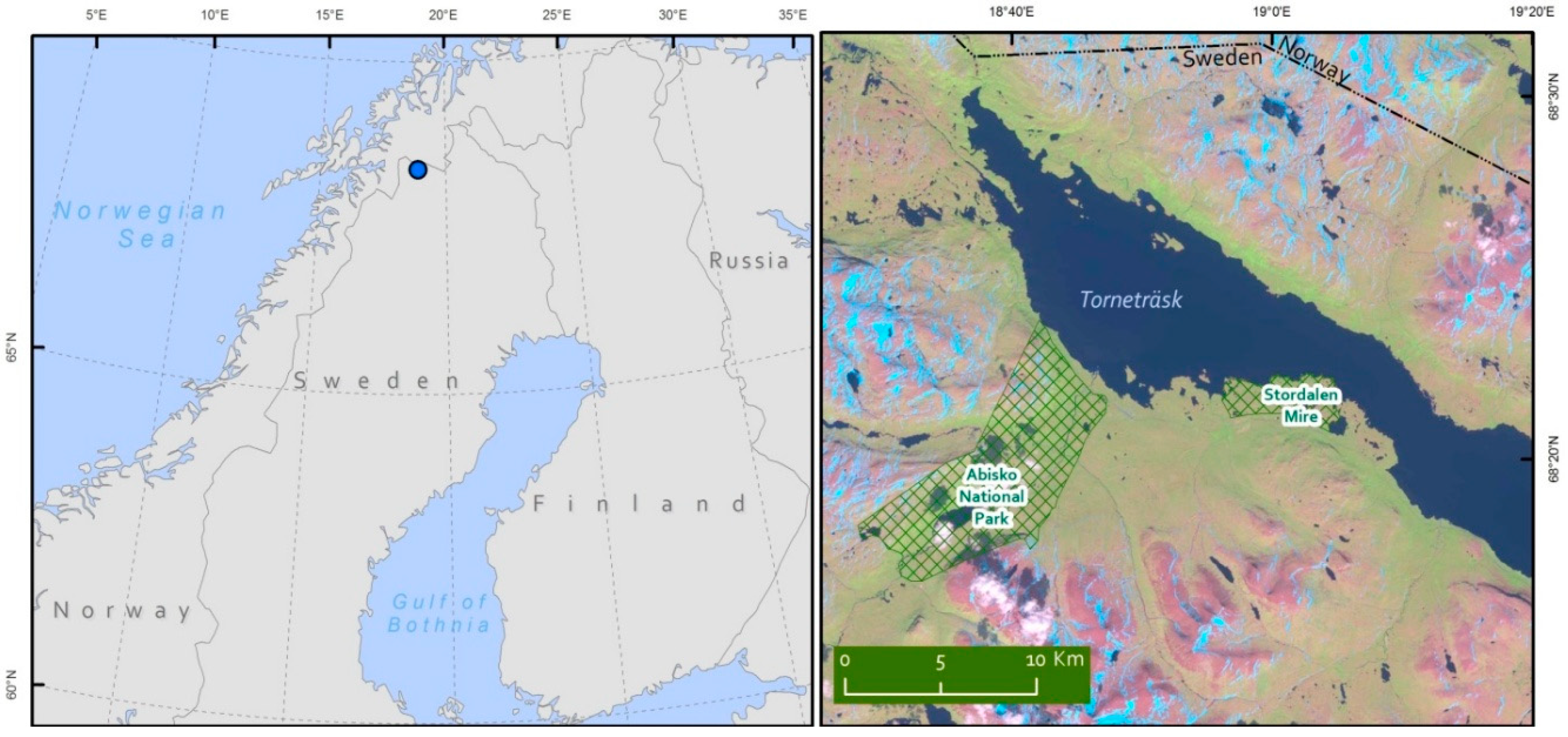
2.1. Study Site

Our study was conducted at Stordalen Mire, a palsa peatland in the discontinuous permafrost zone 11 km east of Abisko, Sweden (68°21′N,18°49′E) (Figure 1). The Abisko Scientific Research Station has supported ecological research and environmental monitoring for over a century, and the nearby Stordalen Mire has been a key research site for the study of the ecological impacts of permafrost degradation [43]. In this system, permafrost loss causes hydrologic and vegetation shifts characterized by the collapse of well-drained permafrost-supported palsas into wetter ecosystems characterized in part by partially thawed moss-dominated (Sphagnum spp.) bogs and fully thawed sedge-dominated (e.g., Eriophorum angustifolium and Carex spp.) fens [2]. Carbon flux measurements (carbon dioxide (CO₂), CH₄, and total hydrocarbons) using static chambers, automatic chambers, and eddy-flux towers have been conducted at this site for several decades and have shown that each habitat type along the thaw gradient has distinctive flux characteristics and that the thaw transition is accompanied by changes in CH₄ and CO₂ fluxes and an overall increase in radiative forcing [3,4,5,8,45].

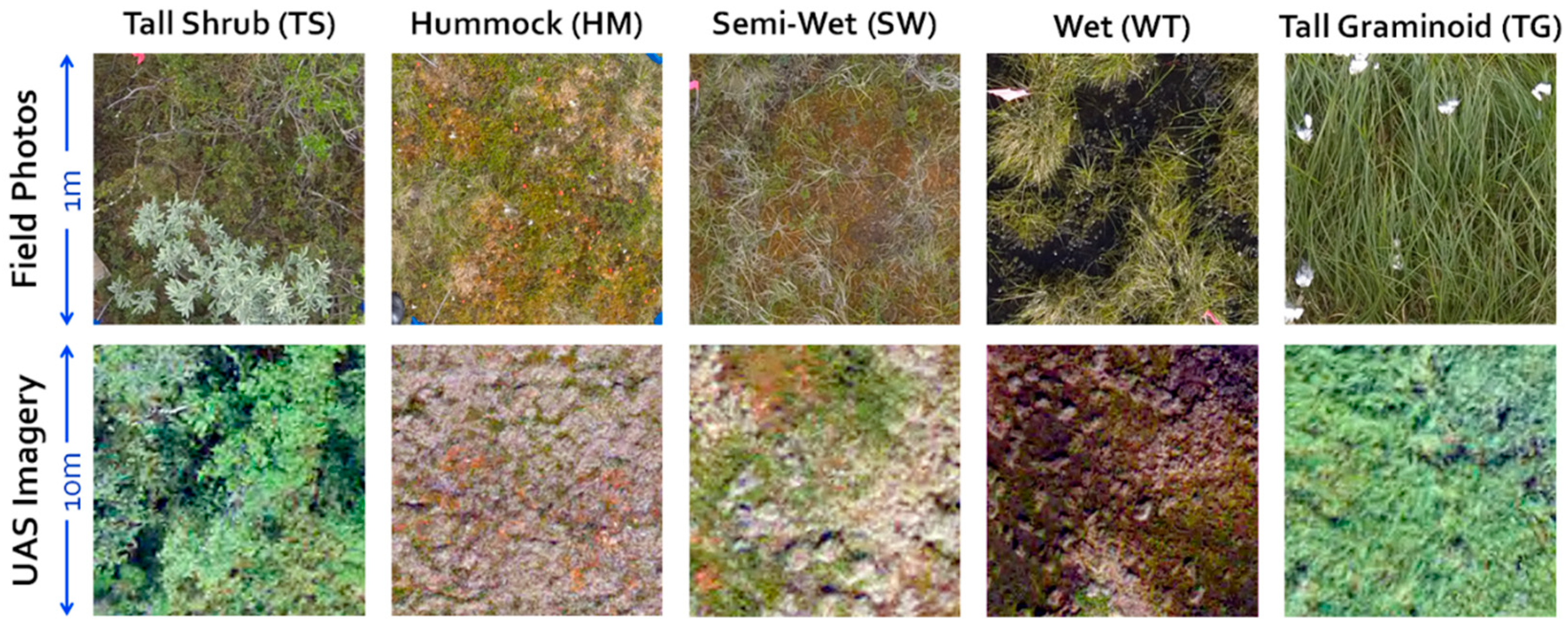
2.2. Vegetation Field Plots

In July 2014, 50 randomized square-meter plots were measured for vegetation composition across the mire and individually classified into one of the five cover types (10 plots in each cover class). Cover type classification of each plot was determined based on vegetation composition and the hydrological state of the landscape. GPS coordinates were collected at all four corners of each plot. These plots represented only a single cover type and did not consist of a mix of two cover types. GPS data collection was not accurate enough to use in model training and prediction. These vegetation field plots were only used in the development of species composition and dominant species for each cover type, as well as to calculate a species richness index. We used Shannon’s index of entropy [46]. To examine the differences in species richness between vegetation cover types, we used a Tukey test with an alpha value of 0.05 for indication of a significant difference. We used connecting letters to indicate differences between groups (

Table 1. Attributes of the five vegetation cover classes in our study. Rock cover type is defined as granite rock and stone pits. The Other cover type is human structures, boardwalk, and buildings.

Cover Type	Soils and Vegetation	Dominant Vegetative Species	%	Second Dominant Vegetative Species	%	Diversity Index	Connecting Letter Report
Tall Shrub	Ombrotrophic, found in dry areas	Dwarf Birch (Betula nana)	18.7	Cloudberry (Rubus chamaemorus)	11.4	1.53	A
Hummock	Ombrotrophic, on permafrost	Crowberry (Empetrum hermaphroditum)	16.9	Hares Tail (Eriophorum vaginatum)	16.1	1.44	A
Semi-Wet	Ombrotrophic or minerotrophic	Spagnum sp.	43.1	Hares Tail (Eriophorum vaginatum)	15.6	0.61	B
Wet	Ombrotrophic	Open Water	43.1	Spagnum	8.2	0.70	B
Tall Graminoid	Wet minerotrophic	Carex sp.	30.7	Cotton Tail (Eriophorum angustafolium)	11.5	0.90	B

).

2.3. UAS Image Data Collection

Aerial images of Stordalen Mire were collected on 11–12 July 2014 using cameras mounted on a fixed-wing unmanned aircraft system. Our choice of these dates was because this is a time of the year when vegetation is green, thaw ponds are evident, and there is no ice or snow. In addition, mid-July is a time of relatively clear and warm weather, allowing for imagery to be collected. This time of year also has a higher sun angle, providing better illumination and less shadow. A total of six flights were conducted during this time frame. The area of interest was an approximately 1 × 0.5 km area of the mire that has been rapidly undergoing permafrost thaw in the last decade and has been highly studied [47]. The fixed-wing plane developed by Robota (www.robota.us) was the Triton XL. This is a small compact vehicle that allows for 0.5 kg of payload. We used the Robota Goose autopilot for automated flight line planning and flight tracking. The autopilots on both UASs provide real-time telemetry of the UAS for tracking of the remaining battery charge, airspeed, altitude, and other UAS diagnostics, allowing for fail-safe flight and planning.

The fixed-wing UAS was flown at a 70-m altitude with a speed of 12 m/s. Flight lines were determined with 50% overlap between images based on designated flight speed, camera view angle, and altitude. Flight lines were extended well past the region of interest to both provide image overlap and avoid angled or oblique images. This overlap allowed for image stitching to be conducted. Imagery was collected using a three-band RGB Panasonic Lumix-GM1. Over 600 images were collected from each 30-min flight, with flights taking place over this two-day period. Flight lines were flown twice and images recorded every 2 s. Flights were begun at 11:30 a.m.

We used Photoscan to also estimate the quality of each image, which examines the sharpness at the most focused region of each picture. Additionally, all images were manually inspected for additional problems, such as tilt or blur, and only clear images were used in the final mosaic. Only images from July 11 were used in our study due to it being cloud free and the least wind during the time of flight. The six hundred images were stitched together using Photoscan Pro 1.2 by AgiSoft (www.agisoft.com) and resulted in a sub-centimeter photo mosaic. For the final product, we used the medium-to-highest setting for all Photoscan image stitching steps. This included Align Photos: Accuracy (High), Pair preselection (Generic), Build Dense Point Cloud: Quality (Medium), Depth Filtering (Aggressive), Build Mesh: Surface Type (Arbitrary), Source Data (Sparse Cloud), Face Count (Medium), Interpolation (Enabled), Build Texture: Mapping Mode (Adaptice Orthophoto), Blending Mode (Mosaic), Texture Size (10,000), and Build Tiled Model: Source Data (Mesh), Pixel Size (0.00074196), Tile Size (8192). An orthomosaic image was rendered from the stitched imagery. Though this resulted in added computational loads, it provided the best image for analysis. Stitching with lower setting was conducted on a laptop at the field site in order to determine if the collection of aerial images provided sufficient overlap (Figure 2).

A total of 457 images were used for stitching and 411 were used in the final stitched image. We used 161,125 tie points and generated a dense point cloud of 50,563,390 points. An orthomosaic image was rendered from final stitched image.

2.4. Georectification

Sixty-four ground control points (GCPs) were distributed throughout 25 hectares of the study area, including approximately 1.3 km of installed raised boardwalk. GCPs were placed strategically at boardwalk intersections or at board crosshatches that would be visible in imagery captured from the UAS. GCP locations were collected in July 2014. GCPs were recorded using a Trimble^® GeoXT™ 6000 handheld GNSS unit. An additional 78 GCPs were collected in July 2015 using a Trimble^® Geo7X GNSS receiver with a Tornado™ external antenna, where location accuracy was low in 2014. These data were corrected for positional accuracy using SWEPOS^® RINEX v2 navigation files collected from a GNSS base station less than 10 km away. GCPs from 2014 collected with differential GNSS had Root Mean Square Error (RMSE) between 36 and 140 cm (mean = 0.63 cm, standard deviation = 0.21 cm). GCPs from 2015 collected with the improved GNSS unit had RMSE +13 cm. The image was further cropped to focus on research sites and a region with less error. The final mosaicked UAS image had spatial dimensions of 0.3 × 0.6 km (14.2 ha) represented by 7724 × 20,357 pixels (Figure 2). Use of these GCPs for image georectification resulted in accuracies that were higher around the boardwalk and decreased in areas further from manmade features and in homogenous areas of vegetation. This corresponds with larger areas of tall grasses, which we attribute to blur caused by wind. We note that the GCPs were not solely limited to the boardwalk and were spread out across the area of study. The corrected GCPs were then used within ArcGIS to georectify the stitched photo mosaic using a second-order polynomial transformation. This allowed for the highest level of accuracy with the least amount of warping of the mosaic. The georectified image had a pixel resolution of 3 cm. Agisoft errors in image stitching were found in homogenous areas, such as water or when the plane banked while collecting images.

2.5. Texture Analysis

Code was developed to examine the relationship between each pixel and its neighbors. This is termed textural analysis and uses the spatial arrangement of pixels to determine additional properties of the image [48,49,50,51,52]. In computer vision applications, texture analysis is often used to segment the image [53,54,55,56]. We calculated entropy (ENT), evenness (EVN), and angular second momentum (ASM) as a moving window (17 × 17 pixels) for every pixel in the fully stitched-together image. The equations for these textural analyses are found in Hall-Beyer [57] and are common equations used in species diversity indices as well [46]. We tested red and blue bands and, due to correlation of spectral bands, we used only the green band for texture analysis used in the statistical model. The mean, mode, maximum, minimum, range, and standard deviation of pixel values were also calculated using the same moving window. These digital image processing routines provided additional metrics used in the development of the statistical model. Our routines were coded with first-order analysis, meaning that all pixels within a moving window were included in the analysis and no other spatial information within that moving window was included. Grey-level co-occurrence matrix (GLCM) often allows for second-order analysis in which the location within the moving window is included as an additional facet of the analysis [57]. With our moving window, the same resolution of the imagery was maintained, as the result of the moving window provided a value for the central pixel. Examples of imagery for the textural analysis are presented in Figure 3. Texture analysis was coded in Python (v. 2.7) using NumPy and SciPy extensions, along with Geospatial Data Abstraction and OGR Simple Feature Libraries.

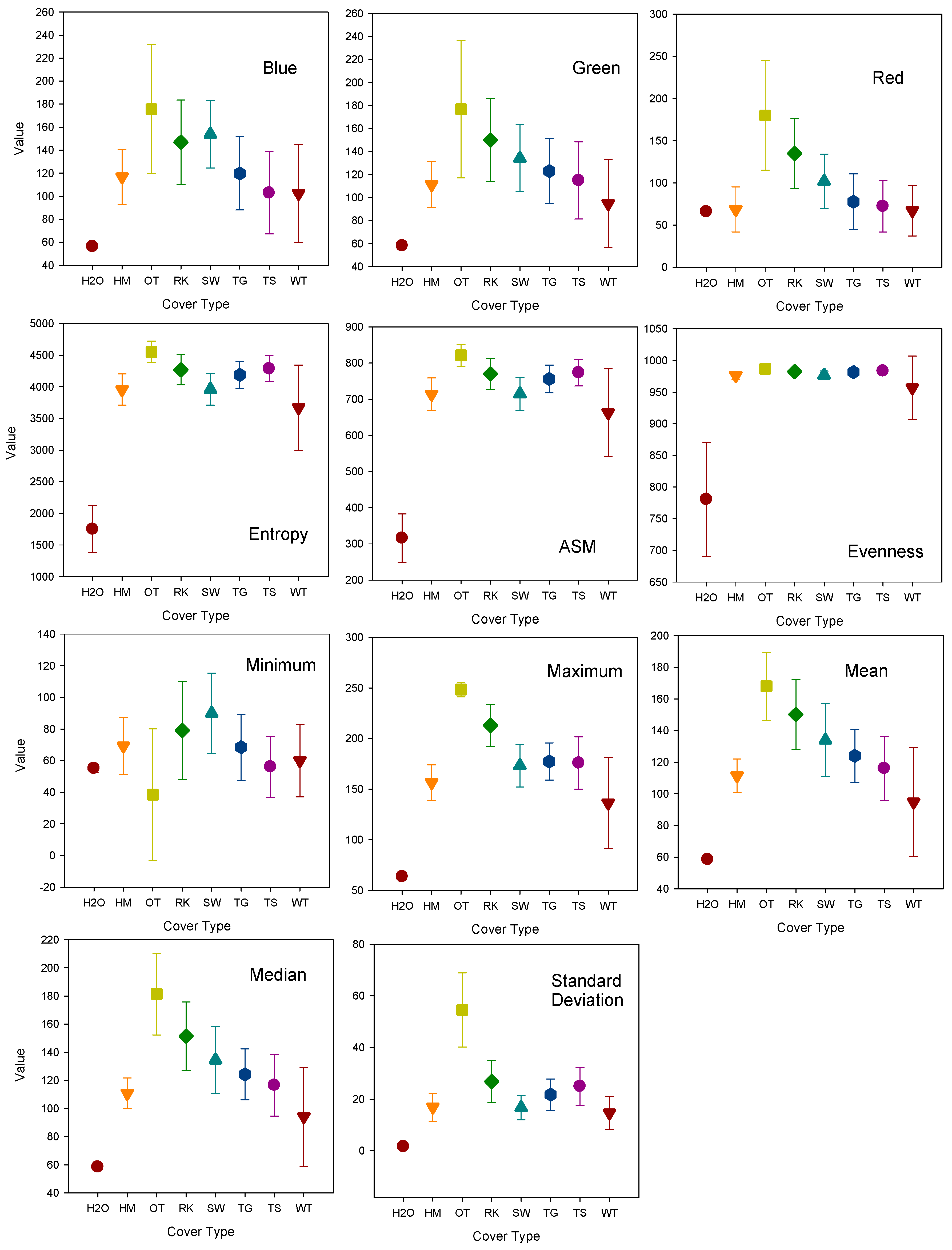
2.6. Data Extraction and Statistical Analysis

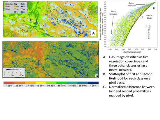
Two hundred randomly selected locations (0.5 × 0.5 m, corresponding to 71 × 71 pixels) were generated over the UAS imagery. Researchers familiar with both the vegetation at Stordalen Mire as well as the general landscape classified each of these training samples as one of eight classes (Figure 2). These classes included five vegetation classes, two nonvegetative classes, and open water (Figure 4. Table 1). All cover classes were represented in the randomly selected manual classified plots. Once the image was clipped, only 114 plots remained in our core region of study. This broke down to the numbers of samples for each cover type, with number in parenthesis: H₂O-Water (3), HM-Hummock (25), OT-Other (3), RK-Rock (5), SW-Semi-Wet (20), TG-Tall Graminoid (24), TS-Tall Shrub (24), and WT-Wet (8). Each plot consisted of 289 pixels with a total of 32,940 pixels with 12 bands used in our classification model. Zonal statistics were used to extract pixel values at these locations along with the user-defined cover class. All pixel values from these locations were imported into JMP Pro 12 statistical software to develop a statistical model for image classification that could then be applied across the entire UAS image. Graphs were generated using SigmaPlot 10.

Data was extracted for the randomly selected plots for manual interpretation into one of the eight cover classes (Figure 3, Figure 4 and Figure 5) and all pixels were extracted within a polygon. Using the data extracted from the imagery and the manually interpreted cover class, we developed a Bayesian artificial neural network [37]. Because training sample locations were randomly selected, no spatial component was included in the analysis. For training, we used 66% of that data and withheld 33% of the data for validation. This is a common split in supervised classification efforts with validation. Our hidden layer structure used five nodes with the hyperbolic tangent function (TanH) (Supplemental Material, Figure S1). We used a squared over-fitting penalty and ran the ANN for 100 tours. A probability map was generated for each of the eight classes (Supplemental Figure S2a–h), with the highest probability for each class indicating the final classification (Figure 6). A confusion matrix allowed us to determine which classes were erroneously classified and to which classes they were assigned. The individual probability maps allow us to also determine the error associated with the overall landcover classification. We report the training and validation confusion matrices as well as statistical estimate of correct class estimation.

In addition to calculating a confusion matrix, we assessed the ANN by calculating the receiver operating characteristic (ROC) to examine the performances of classifiers in discriminating the ANN to predict cover classes [36]. The receiver operating characteristics (ROC) were used to assess the performances of classifiers. The ROC curves represent rapid convergence to the best model among the eight cover classes used, indicating good model prediction (Supplemental Material Figure S2). The ROC uses true negatives, true positives, false negatives, and false positives to determine model prediction rates. A value of 1 indicates extremely good model prediction, while a value of 0.5 is considered to be chance performance.

A generalized r² value was determined for the training and validation datasets as a criterion to determine model strength [58]. Nagelkerke [58] discussed the modification of earlier definitions of r² as an indicator of the proportion of explained variance for different models. Paliwal and Kumar [59] reviewed studies’ statistical techniques for neural networks, assessing the validation methods and error measures, with r² being one of the methods. Others have looked at r² as a method for looking at generalized linear mixed-effects models [60,61]. Our ANN predicted categorical data and Nagelkerke [58] showed that it is possible to calculate an r² value for categorical models. This is sometimes referred to as a Nagelkerke or Craig and Uhler r² [58,62]. The deviation from the true class is used to determine the error in calculating the r² value but is scaled so that a value of one indicates a perfect fit, also known as a Cox and Snell pseudo r² [63]. Other measures of our ANN were also calculated, such as RMSE and an overall misclassification rate. We also calculated commission and omission errors by class. Pontius et al. [64] suggest using a disagreement estimate for accuracy assessment. We determined an overall disagreement estimate which included both quantity and allocation disagreement [64]. We also developed a prediction profiler to examine which parameters were used in determining specific cover classes.

We recoded the ANN in Python (v. 2.7) to classify all pixels in our image (Figure 6). For error estimation, we applied the confusion matrix to each pixel (Figure 7). We also examined the probability for each of the classes and made a composite image of the highest probability, which was used in our final classification for that pixel. In an effort to explore and utilize the multiple probability maps generated by the ANN for each cover class, we developed two methods. First, we calculated the difference between the probability of the highest ranked class and the second ranked class for each pixel. To examine these, we extracted the maximum probability (highest) and the second ranked class probability from the eight different cover type results and present this information as maps (Figure 8a). This is similar to the work done by Tapia and Bijker [65]. Second, we calculated the difference between the two values and generated a normalized difference, where the difference was divided by the highest probability (Figure 8b, Supplemental Material Figures S2–S9). The rationale for this was that although a difference might be small, if the maximum probability is low, the relative probability distance could be as large as two high probabilities. By utilizing two probabilities output from the ANN, we suggest that additional insight into model performance may be gleaned. This method, to look at model predictive confusion, indicates issues in the model when two classes have similar probabilities, indicating that it is harder to discern which is correct and warrants further examination by the researcher. We display these results as maps (Figure 8), scatterplots (Figure 9a,b), and box and whisker plots (Supplemental Material Figures S12 and S13). Our results when viewed across the spatial domain could indicate that certain cover types exhibit patterns of error or confusion reflective in the spatial pattern seen in cover class types.

3. Results

Across the manually interpreted plots, texture and reflectance values varied between and within cover classes for all metrics calculated and pixel values extracted for use in the ANN development (Figure 5). Because these plots were based on the image itself, there was no need to address errors between field plots and image data. Of the vegetation classes, Semi-Wet exhibited the highest green-band reflectance values on average. For textural metrics, Wet vegetation exhibited the lowest entropy, angle of second momentum (ASM), and evenness for vegetation classes, while Tall Shrubs tended to have higher texture values (Figure 6). Texture values were lowest for Water when comparing all classes.

Within the bounds of the image, cover classes indicative of permafrost (indicative of a thin active layer), i.e., Hummock and Tall Shrub, comprised 43.9% of the landscape (Figure 5 and

Table 2. Percentage and pixel number for each of the eight cover classes. H₂O-Water, HM-Hummock, OT-Other, RK-Rock, SW-Semi-Wet, TG-Tall Graminoid, TS-Tall Shrub, WT-Wet.

Cover Type	Abbrev.	Pixels	Percent
Other	OT	1,028,465	0.7%
Rock	RK	4,882,573	3.1%
Tall Graminoid	TG	38,379,784	24.4%
Hummock	HM	42,193,103	26.8%
Tall Shrub	TS	26,852,493	17.1%
Water	H2O	787,946	0.5%
Wet	WT	8,538,871	5.4%
Semi-Wet	SW	34,574,233.	22.0%
Total	TT	157,237,468	100.0%

). Tall Graminoid comprised 24.4% of the total area of our collected image and Semi-Wet was 22.0%. Cover classes of Rock and Other accounted for 3.7% of the landscape area and Water for 0.5% (Figure 5).

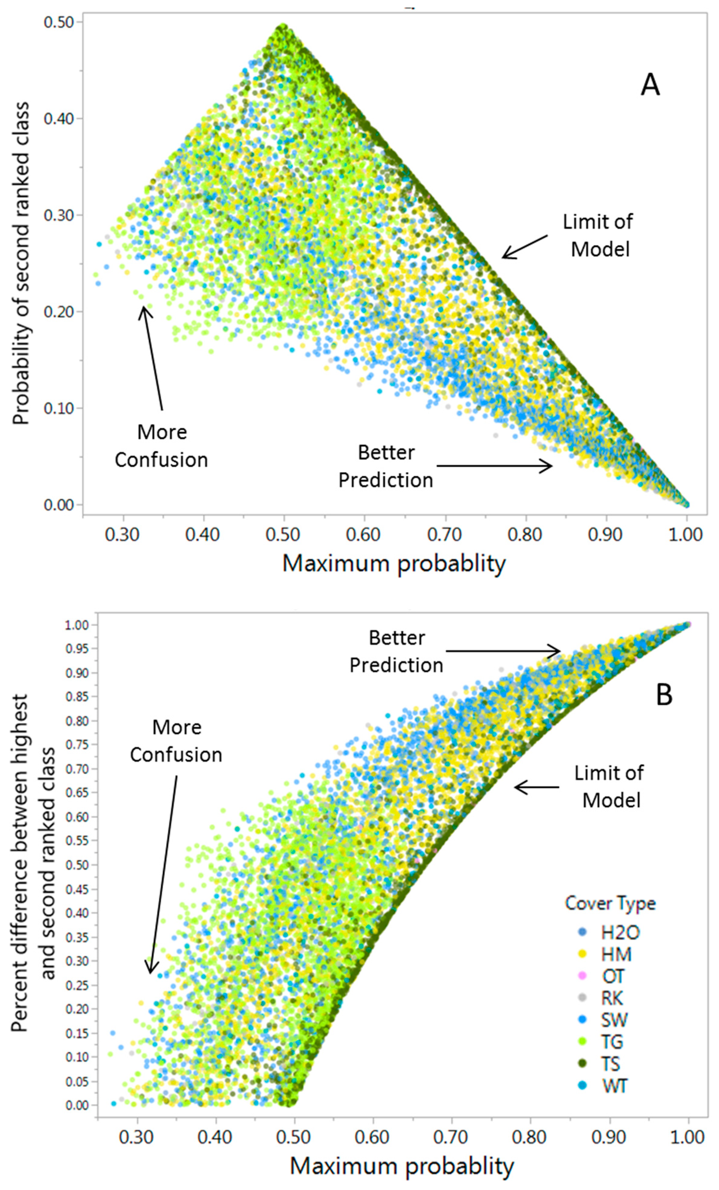
Error Analysis and Cover Class Assessment

Our training dataset had a generalized r² of 0.899 and our validation dataset result was 0.897. Our misclassification rate was 0.319 for our training dataset and 0.323 for the validation dataset. We calculated two different estimates of error from our model. Root mean square error for training was 0.509 and 0.512 for validation. Training and validation data are presented in

Table 3. Confusion matrix for training prediction rates from the ANN for cover type. H₂O-Water, HM-Hummock, OT-Other, RK-Rock, SW-Semi-Wet, TG-Tall Graminoid, TS-Tall Shrub, WT-Wet.

Training Prediction Rate
Classes	H2O	HM	OT	RK	SW	TG	TS	WT
H2O	1.00	0.00	0.00	0.00	0.00	0.00	0.00	0.00
HM	0.00	0.82	0.00	0.00	0.07	0.08	0.02	0.00
OT	0.00	0.00	0.96	0.04	0.00	0.00	0.00	0.00
RK	0.00	0.01	0.02	0.79	0.01	0.03	0.13	0.02
SW	0.00	0.13	0.00	0.01	0.77	0.08	0.00	0.02
TG	0.00	0.13	0.00	0.01	0.11	0.50	0.25	0.00
TS	0.00	0.04	0.00	0.02	0.03	0.32	0.59	0.00
WT	0.00	0.19	0.00	0.00	0.13	0.12	0.01	0.55

and

Table 4. Confusion matrix for validation prediction rates from the ANN for cover type. H₂O-Water, HM-Hummock, OT-Other, RK-Rock, SW-Semi-Wet, TG-Tall Graminoid, TS-Tall Shrub, WT-Wet.

Validation Prediction Rate
Classes	H2O	HM	OT	RK	SW	TG	TS	WT
H2O	1.00	0.00	0.00	0.00	0.00	0.00	0.00	0.00
HM	0.00	0.84	0.00	0.00	0.07	0.08	0.02	0.01
OT	0.00	0.00	0.95	0.05	0.00	0.00	0.00	0.00
RK	0.00	0.01	0.02	0.79	0.01	0.03	0.13	0.02
SW	0.00	0.14	0.00	0.00	0.75	0.08	0.00	0.02
TG	0.00	0.14	0.00	0.00	0.11	0.50	0.25	0.00
TS	0.00	0.04	0.00	0.02	0.03	0.33	0.58	0.00
WT	0.00	0.20	0.00	0.00	0.13	0.11	0.01	0.55

and provide insight into how the ANN performed for specific cover classes and what classes were erroneously assigned for a pixel. Commission and omission errors for each class are presented in

Table 5. Omission and commission errors for each cover class. H₂O-Water, HM-Hummock, OT-Other, RK-Rock, SW-Semi-Wet, TG-Tall Graminoid, TS-Tall Shrub, WT-Wet.

Classes	Training	Error	Validation	Error
	Omission	Comission	Omission	Comission
H2O	0.00	0.00	0.00	0.00
HM	0.29	0.18	0.30	0.16
OT	0.03	0.04	0.02	0.05
RK	0.20	0.21	0.17	0.21
SW	0.29	0.23	0.29	0.25
TG	0.52	0.50	0.52	0.50
TS	0.32	0.41	0.32	0.42
WT	0.13	0.45	0.15	0.46

for both training and validation efforts. Overall classification error was low, except for a few classes. This was primarily due to misclassification between two classes, Tall Graminoid and Tall Shrub. Tall Shrub was often classified as Tall Graminoid, while Tall Graminoid was often interpreted as Hummock or Tall Shrub. The Wet vegetation cover class was often classified as Hummock, Tall Graminoid, or Tall Shrub. All other classes had prediction rates higher that 75% (Table 3). The overall cover classification map is presented in Figure 6. Using the ROC to examine of our models’ predictive power, we found our models predicted well, with class Water being the strongest model and Tall Graminoid being the poorest model (Supplemental Material Figure S10). Our prediction profiler is presented in Supplemental Figure S11 and indicates specific responses of the model’s parameters to estimation of individual cover classes.

We mapped the prediction rate for each class from the ANN confusion matrix using the validation prediction rates (Supplemental Material, Figures S2–S9). This was done for each pixel across the landscape and provides an estimate of overall error that may have been made in the model prediction (Figure 7). The second estimate of error is to map the highest class probability for each pixel based on the ANN (Figure 8a). Each pixel had a probability of being in one of the classes, but we chose the highest class estimate for each pixel to be assigned that class. This provides an estimate of the predictive power of our model across the landscape.

Our method of examining probabilities for the highest and second highest class predictions at the pixel level are presented in Figure 8b,c. These maps indicate areas of red when the individual probabilities of two classes are small. Areas seen in blue are areas that have greater values between the highest and second highest probabilities and are class independent. Scatterplots of data from individual pixels (data from Figure 8a–c) are presented in Figure 9a,b. These plots indicate the limits of the model, better predictive regimes, and pixels that exhibit confusion because the probability space is similar between the best predictive classes. Colors of individual points in the scatterplots indicate cover class.

4. Discussion

Image Classification and Error Estimates

Our efforts to develop techniques for UAS-based mapping and cover type classification provided a robust, inexpensive, and repeatable method for examining subarctic vegetation in peatlands. Cover classes have an advantage for scaling to new areas and linkage to coarser-resolution remote sensing [21]. Because functional cover types have been linked to CH₄ emissions in high latitudes, mapping vegetation using broad cover types that are related to CH₄ emissions is useful for understanding landscape change and provides context and evidence for changes in fluxes related to climate change as well as ties to field observations [3,42,66].

The spatial resolution of the UAS collection and subsequent georeferencing of the image provided the ability to examine the complex spatial heterogeneity of vegetation across the mire. The textural analysis that we used expanded upon the three optical bands, which are often highly correlated. The majority of the eight cover types had low misclassification rates. The ROC and AUC values indicated that the model was predicting better than random. A confusion matrix helped to identify issues with discriminating between Tall Graminoid and Tall Shrub classes.

The prediction profiler indicates that Water was classified primarily by one variable—Evenness. Some cover classes, like Other and Rock, primarily leveraged two remote sensing variables in the ANN. Hummock and Tall Graminoid show responses in model prediction from almost all remote sensing parameters. Cover types that leverage more variables indicated from the prediction profiler primarily had higher misclassification rates, indicating that these cover types might be more complex, both in species and structural diversity. This is supported in the species richness values in Table 1 for the cover types. Tall Shrub and Hummock had significantly higher diversity indices than the three other classes when compared using a Tukey test (Table 1). Understanding these complexities in classification could provide insight into what additional variables could be derived that might further improve classification for those specific cover types.

Water had the lowest omission and commission errors for both training and validation results, with no pixels being erroneously assigned. The Other cover class had the next lowest error in classification. These two cover classes tend to be defined by smooth, even pixel variation and relied on the texture features in the prediction profiler. We suggest that texture features are useful indicators of these classes and could be used singularly if only those cover classes were necessary to quantify in the landscape. The highest errors were found for Tall Graminoid. The Wet cover class had differences between omission and commission errors (0.13, 0.45 training and 0.15, 0.46 validation). This indicates that less Wet pixels were omitted in prediction but more pixels of other classes were erroneously assigned the Wet cover class. The number of samples differed between classes. Water, Rock, and Other had low sample numbers by high classification rates. This suggests that sampling these cover classes might not require as many samples as other cover classes. The Wet cover class only had eight plot samples and though the number of pixels was 2312 used in the ANN, they might still might have been improved with a higher number of samples in this class. We suggest that using the omission and commission errors can provide insight into cover class model strengths and weaknesses when used in conjunction with the prediction profiler. Our method for looking at confusion predictions based on the two highest probable cover classes for a pixel provide addition insight.

By comparing the two highest probable cover class values from the ANN, it is possible to determine when the model distinctions in predictive power between two classes are low at the pixel level. This has been defined as confusion estimate in defining predictive power for a model, again at an individual pixel level between two classes [65]. Tapia and Bijker [65] used a K-means unsupervised classification to determine the ideal number of classes when analyzing continuous variables (topography, slope, and normalized difference vegetation index). They termed this a confusion estimate and used it to develop a sampling strategy. We used the confusion estimate in an effort to examine model results for cover classes that have potential problems and as a means to suggest further remote sensing analytical development for those classes. We also plotted our results as a scatter plot, allowing for use to discern areas of confusion for cover classes. Finally, we developed a normalized confusion estimate because the probability distances between two classes that are 90% and 80% are not different than two classes that are 45% and 40%. This rationale is that though the model prediction might be low, it is still much better than the second best classification probability. Figure 9a,b shows areas in the scatterplot where the model provides better prediction and areas in the scatterplot that are more prone to confusion. Both the omission and commission error calculations and our estimate of difference between model predictive probabilities on a pixel level still require the need for interpretation and understanding based on field-based data. Even though our model has high spatial resolution at 3 cm, structural components of vegetative species may display a mix of optical properties or similarity between species.

A confusion matrix (Table 3 and Table 4) showed issues with determining Tall Graminoid and Tall Shrub classes, which were often classified as each other. This misclassification may be due to both classes containing a species from the same genus, both which look similar from an aerial view. The Tall Graminoid cover class consists of open water, Carex spp., and E. angustifolium, with E. angustifolium being the majority. The Tall Shrub cover class consists of mainly Betula nana and Betula pubescens, however, Eriophorum vaginatum is often found mixed in with the birch shrubs. E. angustifolium and E. vaginatum differ from one another in their habitat and morphology. E. angustifolium has multiple flower heads and grows from rhizomes, while E. vaginatum has a single flower head and grows from dense tussocks (Figure 10). The imagery was unable to differentiate between the number of flower heads, thus misclassifying the Tall Graminoid and Tall Shrub classes. These two species also differ in height. E. vaginatum grows 30–50 cm high (Wein 1973), while E. angustifolium grows 60–100 cm high (Wein 1973). The tall thin linear vegetation structure was similar to Carex spp. and our texture analysis appears to have results that were similar for two very different cover types.

Topography is a key feature in the permafrost collapse transition for vegetation cover, primarily due to changes in the hydrology and inundation to water. Lidar has been used for understanding forest structure and estimating microtopography [17,67,68,69], and specifically at Abisko and Stordalen, Sweden, it was used in a cover type classification [19]. This is a highly useful method for classification of mires and fens but is expensive and requires computation time and expertise in analysis [27]. In addition, optical spectra are often not included with such lidar collections and thus vegetation cover may be difficult to discern. In future efforts, we suggest using optical imagery from a UAS with overlapping images to examine the use of parallax and use Structure from Motion (SfM). From this, a plant height model can be developed which may be used as an additional component in the machine learning analysis [28].

The UAS imagery we collected does not include topography; therefore, vegetation height was not used for the classification process. Since the most easily distinguishable difference between E. angustifolium and E. vaginatum is plant height, topographical analyses may aid in the separation of the Tall Shrub and Tall Graminoid cover classes [44]. Malhotra et al. [44] showed that microtopography is related to litter decomposition rates, further suggesting the importance of topographic data from a UAS in the understanding other ecosystem processes. The confusion between the two aforementioned classes (Tall Shrub and Tall Graminoid) may be due to the difficulty in collecting tall shrub plots in the field, thus underclassifying this cover type. B. pubescens ssp. czerepanovii grows as tall as 5–7 feet at Stordalen Mire; therefore, it was not practicable to place the quadrat on these taller shrubs. If plots were able to be collected at these taller shrubs and thus be used for classification, then the Tall Shrub cover class may have been better differentiated.

Environments like Stordalen Mire are associated with inconsistencies in UAS image data acquisition caused by blur from wind, poor light conditions, and cloud cover. An examination of Landsat imagery at Stordalen Mire over 35 years (1984–2018) (1624 images) indicates that at the collection time, image tiles have an average of 57% cloud cover (Supplemental Material, Table S1). This stresses the opportunistic advantage of UAS image collection at a specific location, with flying specific clear days and even flying between passing clouds. To overcome these issues, we conducted flights as close to solar noon as possible and made multiple passes over the area of interest. We stress that multiple overpasses to collect images provides more data than is necessary but maximizes the coverage area with quality images, while only marginally increasing the amount of time spent in the field and the burden on the UAS.

Collection of data even without the ideal sensor package or issues with georeferencing still provides an important contribution to the long-term understanding of a site. It is far better to have some imagery than none, but we do stress the need to utilize best practices for georeferencing and transparency in classification methods. ANN is sometimes considered a black box, but with presenting software and parameter settings along with training and validation methodology, such a process can be repeatable. We also suggest the use of other machine learning techniques such as random forest for classification efforts. The characterization of this mire provides a much needed high-resolution classification of this study site to examine submeter vegetation change associated with permafrost thaw and collapse.

5. Conclusions

Arctic peatlands, including fens and mires, have great spatial heterogeneity in regard to vegetation composition. Vegetative species have been tied to biogeochemical processes through associative vegetation cover classes that have been instrumented and measured. Cover classes are advantageous as they allow scaling and linkages to biogeochemical measurements and modeling efforts and allow application to new locations. These species often are structurally similar across locations, allowing for UAS classification to be a robust method for high-resolution image classification. We used a simple RGB camera with texture analysis to develop an ANN to provide a cover classification map with error estimates. Textural analysis of the image provided additional metrics for classification and showed importance when classifying specific classes. Misclassification rates were higher for specific classes, indicating a need for additional field plots as well as the potential value of using topographic estimates provided by parallax on stereo images or lidar data. Presentation of probability maps for the highest and second highest classes and difference between these two classes provides a method for presenting the confusion of classification on a pixel by pixel level, allowing for cover type and spatial influences on classification to be examined. We have developed a high spatial resolution (3 cm) cover classification that focuses on vegetation cover types that represent biogeochemical processes related to CH₄ production. Our classification provides a contemporary dataset to be used along with ongoing field measurements that can be compared with historical classification efforts at the site.

References

1. Schuur, E.A.G.; McGuire, A.D.; Schädel, C.; Grosse, G.; Harden, J.W.; Hayes, D.J.; Hugelius, G.; Koven, C.D.; Kuhry, P.; Lawrence, D.M.; et al. Climate change and the permafrost carbon feedback. Nature 2015, 520, 171. [Google Scholar] [CrossRef] [PubMed]
2. Johansson, T.; Malmer, N.; Crill, P.M.; Friborg, T.; ÅKerman, J.H.; Mastepanov, M.; Christensen, T.R. Decadal vegetation changes in a northern peatland, greenhouse gas fluxes and net radiative forcing. Glob. Chang. Biol. 2006, 12, 2352–2369. [Google Scholar] [CrossRef]
3. Christensen, T.R.; Johansson, T.; Åkerman, H.J.; Mastepanov, M.; Malmer, N.; Friborg, T.; Crill, P.; Svensson, B.H. Thawing sub-arctic permafrost: Effects on vegetation and methane emissions. Hydrol. Land Surf. Stud. 2004, 31. [Google Scholar] [CrossRef] [Green Version]
4. Bäckstrand, K.; Crill, P.M.; Jackowicz-Korczyñski, M.; Mastepanov, M.; Christensen, T.R.; Bastviken, D. Annual carbon gas budget for a subarctic peatland, Northern Sweden. Biogeosciences 2010, 7, 95–108. [Google Scholar] [CrossRef] [Green Version]
5. Malhotra, A.; Roulet, N.T. Environmental correlates of peatland carbon fluxes in a thawing landscape: Do transitional thaw stages matter? Biogeosciences 2015, 12, 3119–3130. [Google Scholar] [CrossRef]
6. Hodgkins, S.B.; Tfaily, M.M.; McCalley, C.K.; Logan, T.A.; Crill, P.M.; Saleska, S.R.; Rich, V.I.; Chanton, J.P. Changes in peat chemistry associated with permafrost thaw increase greenhouse gas production. Proc. Natl. Acad. Sci. USA 2014, 111, 5819–5824. [Google Scholar] [CrossRef] [PubMed] [Green Version]
7. Ström, L.; Mastepanov, M.; Christensen, T.R.J.B. Species-specific Effects of Vascular Plants on Carbon Turnover and Methane Emissions from Wetlands. Biogeochemistry 2005, 75, 65–82. [Google Scholar] [CrossRef]
8. McCalley, C.K.; Woodcroft, B.J.; Hodgkins, S.B.; Wehr, R.A.; Kim, E.-H.; Mondav, R.; Crill, P.M.; Chanton, J.P.; Rich, V.I.; Tyson, G.W.; et al. Methane dynamics regulated by microbial community response to permafrost thaw. Nature 2014, 514, 478. [Google Scholar] [CrossRef] [PubMed]
9. Chambers, J.Q.; Asner, G.P.; Morton, D.C.; Anderson, L.O.; Saatchi, S.S.; Espirito-Santo, F.D.; Palace, M.; Souza, C., Jr. Regional ecosystem structure and function: Ecological insights from remote sensing of tropical forests. Trends Ecol. Evol. 2007, 22, 414–423. [Google Scholar] [CrossRef] [PubMed]
10. Harris, A.; Bryant, R.G. A multi-scale remote sensing approach for monitoring northern peatland hydrology: Present possibilities and future challenges. J. Environ. Manag. 2009, 90, 2178–2188. [Google Scholar] [CrossRef] [PubMed]
11. Hill, M.J.; Zhou, Q.; Sun, Q.; Schaaf, C.B.; Palace, M. Relationships between vegetation indices, fractional cover retrievals and the structure and composition of Brazilian Cerrado natural vegetation. Int. J. Remote Sens. 2017, 38, 874–905. [Google Scholar] [CrossRef]
12. Morton, D.C.; Nagol, J.; Carabajal, C.C.; Rosette, J.; Palace, M.; Cook, B.D.; Vermote, E.F.; Harding, D.J.; North, P.R.J. Amazon forests maintain consistent canopy structure and greenness during the dry season. Nature 2014, 506, 221. [Google Scholar] [CrossRef] [PubMed]
13. McMichael, C.H.; Bush, M.B.; Silman, M.R.; Piperno, D.R.; Raczka, M.; Lobato, L.C.; Zimmerman, M.; Hagen, S.; Palace, M. Historical fire and bamboo dynamics in western Amazonia. J. Biogeogr. 2012, 40, 299–309. [Google Scholar] [CrossRef]
14. Palace, M.W.; McMichael, C.N.H.; Braswell, B.H.; Hagen, S.C.; Bush, M.B.; Neves, E.; Tamanaha, E.; Herrick, C.; Frolking, S. Ancient Amazonian populations left lasting impacts on forest structure. Ecosphere 2017, 8, e02035. [Google Scholar] [CrossRef] [Green Version]
15. Lees, K.J.; Quaife, T.; Artz, R.R.E.; Khomik, M.; Clark, J.M. Potential for using remote sensing to estimate carbon fluxes across northern peatlands—A review. Sci. Total Environ. 2018, 615, 857–874. [Google Scholar] [CrossRef] [PubMed]
16. Liu, Y.; Key, J.R. Assessment of Arctic Cloud Cover Anomalies in Atmospheric Reanalysis Products Using Satellite Data. J. Clim. 2016, 29, 6065–6083. [Google Scholar] [CrossRef]
17. Arroyo-Mora, J.P.; Kalacska, M.; Soffer, R.J.; Moore, T.R.; Roulet, N.T.; Juutinen, S.; Ifimov, G.; Leblanc, G.; Inamdar, D. Airborne Hyperspectral Evaluation of Maximum Gross Photosynthesis, Gravimetric Water Content, and CO2 Uptake Efficiency of the Mer Bleue Ombrotrophic Peatland. Remote Sens. 2018, 10, 565. [Google Scholar] [CrossRef]
18. Pellissier, P.A.; Ollinger, S.V.; Lepine, L.C.; Palace, M.W.; McDowell, W.H. Remote sensing of foliar nitrogen in cultivated grasslands of human dominated landscapes. Remote Sens. Environ. 2015, 167, 88–97. [Google Scholar] [CrossRef] [Green Version]
19. Siewert, M.B. High-resolution digital mapping of soil organic carbon in permafrost terrain using machine learning: A case study in a sub-Arctic peatland environment. Biogeosciences 2018, 15, 1663–1682. [Google Scholar] [CrossRef]
20. Malmer, N.; Johansson, T.; Olsrud, M.; Christensen, T.R. Vegetation, climatic changes and net carbon sequestration in a North-Scandinavian subarctic mire over 30 years. Glob. Chang. Biol. 2005, 11, 1895–1909. [Google Scholar] [CrossRef]
21. Virtanen, T.; Ek, M. The fragmented nature of tundra landscape. Int. J. Appl. Earth Obs. 2014, 27, 4–12. [Google Scholar] [CrossRef]
22. Lovitt, J.; Rahman, M.M.; Saraswati, S.; McDermid, G.J.; Strack, M.; Xu, B. UAV Remote Sensing Can Reveal the Effects of Low-Impact Seismic Lines on Surface Morphology, Hydrology, and Methane (CH4) Release in a Boreal Treed Bog. J. Geophys. Res.-Biogeosci. 2018, 123, 1117–1129. [Google Scholar] [CrossRef]
23. Rahman, M.M.; McDermid, G.J.; Strack, M.; Lovitt, J. A New Method to Map Groundwater Table in Peatlands Using Unmanned Aerial Vehicles. Remote Sens. 2017, 9, 1057. [Google Scholar] [CrossRef]
24. Anderson, K.; Gaston, K.J. Lightweight unmanned aerial vehicles will revolutionize spatial ecology. Front. Ecol. Environ. 2013, 11, 138–146. [Google Scholar] [CrossRef] [Green Version]
25. Marris, E. Drones in science: Fly, and bring me data. Nature 2013, 498, 156–158. [Google Scholar] [CrossRef] [PubMed] [Green Version]
26. Bemis, S.P.; Micklethwaite, S.; Turner, D.; James, M.R.; Akciz, S.; Thiele, S.T.; Bangash, H.A. Ground-based and UAV-Based photogrammetry: A multi-scale, high-resolution mapping tool for structural geology and paleoseismology. J. Struct. Geol. 2014, 69, 163–178. [Google Scholar] [CrossRef]
27. Turner, D.; Lucieer, A.; Watson, C. An Automated Technique for Generating Georectified Mosaics from Ultra-High Resolution Unmanned Aerial Vehicle (UAV) Imagery, Based on Structure from Motion (SfM) Point Clouds. Remote Sens. 2012, 4, 1392–1410. [Google Scholar] [CrossRef] [Green Version]
28. Sona, G.; Pinto, L.; Pagliari, D.; Passoni, D.; Gini, R. Experimental analysis of different software packages for orientation and digital surface modelling from UAV images. Earth Sci. Inf. 2014, 7, 97–107. [Google Scholar] [CrossRef]
29. Laliberte, A.S.; Goforth, M.A.; Steele, C.M.; Rango, A. Multispectral Remote Sensing from Unmanned Aircraft: Image Processing Workflows and Applications for Rangeland Environments. Remote Sens. 2011, 3, 2529–2551. [Google Scholar] [CrossRef] [Green Version]
30. Strahler, A.H.; Woodcock, C.E.; Smith, J.A. On the nature of models in remote sensing. Remote Sens. Environ. 1986, 20, 121–139. [Google Scholar] [CrossRef]
31. Frolking, S.; Palace, M.W.; Clark, D.B.; Chambers, J.Q.; Shugart, H.H.; Hurtt, G.C. Forest disturbance and recovery: A general review in the context of spaceborne remote sensing of impacts on aboveground biomass and canopy structure. J. Geophys. Res.-Biogeosci. 2009, 114. [Google Scholar] [CrossRef] [Green Version]
32. Xie, Y.; Sha, Z.; Yu, M. Remote sensing imagery in vegetation mapping: A review. J. Plant Ecol. 2008, 1, 9–23. [Google Scholar] [CrossRef]
33. Pal, M. Random forest classifier for remote sensing classification. Int. J. Remote Sens. 2005, 26, 217–222. [Google Scholar] [CrossRef]
34. Pal, M.; Mather, P.M. Support vector machines for classification in remote sensing. Int. J. Remote Sens. 2005, 26, 1007–1011. [Google Scholar] [CrossRef]
35. Cracknell, M.J.; Reading, A.M. Geological mapping using remote sensing data: A comparison of five machine learning algorithms, their response to variations in the spatial distribution of training data and the use of explicit spatial information. Comput. Geosci. 2014, 63, 22–33. [Google Scholar] [CrossRef]
36. Englemann, B.; Hayden, E.; Tasche, D. Measuring the Discriminative Power of Rating Systems. In Discussion Paper Series 2: Banking and Financial Studies; Deutsche Bundesbank: Frankfurt am Main, Germany, 2003; p. 24. [Google Scholar]
37. Mahmon, N.A.; Ya’acob, N. A review on classification of satellite image using Artificial Neural Network (ANN). In Proceedings of the 2014 IEEE 5th Control and System Graduate Research Colloquium, Shah Alam, Malaysia, 11–12 August 2014; pp. 153–157. [Google Scholar]
38. Atkinson, P.M.; Tatnall, A.R.L. Introduction Neural networks in remote sensing. Int. J. Remote Sens. 1997, 18, 699–709. [Google Scholar] [CrossRef]
39. Nogueira, K.; Penatti, O.A.B.; dos Santos, J.A. Towards better exploiting convolutional neural networks for remote sensing scene classification. Pattern Recognit. 2017, 61, 539–556. [Google Scholar] [CrossRef] [Green Version]
40. Turner, D.; Lucieer, A.; Malenovský, Z.; King, D.; Robinson, S. Spatial Co-Registration of Ultra-High Resolution Visible, Multispectral and Thermal Images Acquired with a Micro-UAV over Antarctic Moss Beds. Remote Sens. 2014, 6, 4003–4024. [Google Scholar] [CrossRef] [Green Version]
41. Wang, R.; Gamon, J.A.; Cavender-Bares, J.; Townsend, P.A.; Zygielbaum, A.I. The spatial sensitivity of the spectral diversity–biodiversity relationship: An experimental test in a prairie grassland. Ecol. Appl. 2017, 28, 541–556. [Google Scholar] [CrossRef] [PubMed]
42. Treat, C.C.; Marushchak, M.E.; Voigt, C.; Zhang, Y.; Tan, Z.; Zhuang, Q.; Virtanen, T.A.; Räsänen, A.; Biasi, C.; Hugelius, G.; et al. Tundra landscape heterogeneity, not inter-annual variability, controls the decadal regional carbon balance in the Western Russian Arctic. Glob. Chang. Biol. 2018. [Google Scholar] [CrossRef] [PubMed]
43. Jonasson, C.; Sonesson, M.; Christensen, T.R.; Callaghan, T.V. Environmental monitoring and research in the Abisko area-an overview. Ambio 2012, 41 (Suppl. 3), 178–186. [Google Scholar] [CrossRef]
44. Malhotra, A.; Moore, T.R.; Limpens, J.; Roulet, N.T. Post-thaw variability in litter decomposition best explained by microtopography at an ice-rich permafrost peatland. Arct. Antarct. Alp. Res. 2018, 50, e1415622. [Google Scholar] [CrossRef]
45. Jackowicz-Korczyński, M.; Christensen, T.R.; Bäckstrand, K.; Crill, P.; Friborg, T.; Mastepanov, M.; Ström, L. Annual cycle of methane emission from a subarctic peatland. J. Geophys. Res.-Biogeosci. 2010, 115. [Google Scholar] [CrossRef] [Green Version]
46. Mouillot, D.; Leprêtre, A. A comparison of species diversity estimators. Res. Popul. Ecol. 1999, 41, 203–215. [Google Scholar] [CrossRef]
47. Lupascu, M.; Wadham, J.L.; Hornibrook, E.R.C.; Pancost, R.D. Temperature Sensitivity of Methane Production in the Permafrost Active Layer at Stordalen, Sweden: A Comparison with Non-permafrost Northern Wetlands. Arct. Antarct. Alp. Res. 2012, 44, 469–482. [Google Scholar] [CrossRef] [Green Version]
48. Haralick, R.M. Statistical and structural approaches to texture. Proc. IEEE 1979, 67, 786–804. [Google Scholar] [CrossRef]
49. Haralick, R.M.; Shanmugam, K.; Dinstein, I. Textural Features for Image Classification. IEEE Trans. Syst. Man Cyb. 1973, SMC-3, 610–621. [Google Scholar] [CrossRef]
50. Soares, J.V.; Rennó, C.D.; Formaggio, A.R.; da Costa Freitas Yanasse, C.; Frery, A.C. An investigation of the selection of texture features for crop discrimination using SAR imagery. Remote Sens. Environ. 1997, 59, 234–247. [Google Scholar] [CrossRef]
51. Hudak, A.T.; Wessman, C.A. Textural Analysis of Historical Aerial Photography to Characterize Woody Plant Encroachment in South African Savanna. Remote Sens. Environ. 1998, 66, 317–330. [Google Scholar] [CrossRef]
52. Ouma, Y.O.; Tetuko, J.; Tateishi, R. Analysis of co-occurrence and discrete wavelet transform textures for differentiation of forest and non-forest vegetation in very-high-resolution optical-sensor imagery. Int. J. Remote Sens. 2008, 29, 3417–3456. [Google Scholar] [CrossRef]
53. Palace, M.; Keller, M.; Asner, G.P.; Hagen, S.; Braswell, B. Amazon Forest Structure from IKONOS Satellite Data and the Automated Characterization of Forest Canopy Properties. Biotropica 2007, 40, 141–150. [Google Scholar] [CrossRef]
54. Gonzalez, P.; Asner, G.P.; Battles, J.J.; Lefsky, M.A.; Waring, K.M.; Palace, M. Forest carbon densities and uncertainties from Lidar, QuickBird, and field measurements in California. Remote Sens. Environ. 2010, 114, 1561–1575. [Google Scholar] [CrossRef]
55. Ahmed, A.; Gibbs, P.; Pickles, M.; Turnbull, L. Texture analysis in assessment and prediction of chemotherapy response in breast cancer. J. Magn. Reson. Imaging 2013, 38, 89–101. [Google Scholar] [CrossRef] [PubMed]
56. Yuan, J.; Wang, D.; Li, R. Remote Sensing Image Segmentation by Combining Spectral and Texture Features. IEEE Trans. Geosci. Remote 2014, 52, 16–24. [Google Scholar] [CrossRef]
57. Hall-Beyer, M. Practical guidelines for choosing GLCM textures to use in landscape classification tasks over a range of moderate spatial scales. Int. J. Remote Sens. 2017, 38, 1312–1338. [Google Scholar] [CrossRef]
58. Nagelkerke, N.J.D. A note on a general definition of the coefficient of determination. Biometrika 1991, 78, 691–692. [Google Scholar] [CrossRef]
59. Paliwal, M.; Kumar, U.A. Neural networks and statistical techniques: A review of applications. Expert Syst. Appl. 2009, 36, 2–17. [Google Scholar] [CrossRef]
60. Guisan, A.; Zimmermann, N.E. Predictive habitat distribution models in ecology. Ecol. Model. 2000, 135, 147–186. [Google Scholar] [CrossRef]
61. Nakagawa, S.; Schielzeth, H. A general and simple method for obtaining R2 from generalized linear mixed-effects models. Methods Ecol. Evol. 2012, 4, 133–142. [Google Scholar] [CrossRef]
62. Cragg, J.G.; Uhler, R.S. The Demand for Automobiles. Can. J. Econ. Rev. Can. d’Econ. 1970, 3, 386–406. [Google Scholar] [CrossRef]
63. Cox, D.R.; Snell, E.J. The Analysis of Binary Data, 2nd ed.; Chapman and Hall/CRC: London, UK, 1989; p. 240. [Google Scholar]
64. Pontius, R.G.; Millones, M. Death to Kappa: Birth of quantity disagreement and allocation disagreement for accuracy assessment. Int. J. Remote Sens. 2011, 32, 4407–4429. [Google Scholar] [CrossRef]
65. Tapia, R.; Stein, A.; Bijker, W. Optimization of sampling schemes for vegetation mapping using fuzzy classification. Remote Sens. Environ. 2005, 99, 425–433. [Google Scholar] [CrossRef]
66. Mikola, J.; Virtanen, T.; Linkosalmi, M.; Vähä, E.; Nyman, J.; Postanogova, O.; Räsänen, A.; Kotze, D.J.; Laurila, T.; Juutinen, S.; et al. Spatial variation and linkages of soil and vegetation in the Siberian Arctic tundra—Coupling field observations with remote sensing data. Biogeosciences 2018, 15, 2781–2801. [Google Scholar] [CrossRef]
67. Palace, M.W.; Sullivan, F.B.; Ducey, M.J.; Treuhaft, R.N.; Herrick, C.; Shimbo, J.Z.; Mota-E-Silva, J. Estimating forest structure in a tropical forest using field measurements, a synthetic model and discrete return lidar data. Remote Sens. Environ. 2015, 161, 1–11. [Google Scholar] [CrossRef]
68. Palace, M.; Sullivan, F.B.; Ducey, M.; Herrick, C. Estimating Tropical Forest Structure Using a Terrestrial Lidar. PLoS ONE 2016, 11, e0154115. [Google Scholar] [CrossRef] [PubMed]
69. Howey, M.C.L.; Sullivan, F.B.; Tallant, J.; Kopple, R.V.; Palace, M.W. Detecting Precontact Anthropogenic Microtopographic Features in a Forested Landscape with Lidar: A Case Study from the Upper Great Lakes Region, AD 1000–1600. PLoS ONE 2016, 11, e0162062. [Google Scholar] [CrossRef] [PubMed]
Figure 1. Overview of study region (left) and Abisko region (right, Landsat FCC); aerial image of study area in Stordalen Mire acquired from an unmanned aerial system (UAS) (far right).
Remotesensing 10 01498 g001
Figure 2. Location of training samples across the Stordalen Mire, Sweden.
Remotesensing 10 01498 g002
Figure 3. UAS imagery collected over a research shack at Stordalen Mire. Left is RGB imagery and the right is entropy calculated on a 17 × 17 pixel moving window on just the green band.
Remotesensing 10 01498 g003
Figure 4. Five vegetation cover classes determined in our study. They range from permafrost to thawed peat, forming wetlands with carex or tall graminoid as the dominate species. Additional land cover types included water, rock, and other (usually manmade structures and research equipment).
Remotesensing 10 01498 g004
Figure 5. Image band and textural analyzed raster data used in our artificial neural network (ANN) determining eight cover types. H2O-Water, HM-Hummock, OT-Other, RK-Rock, SW-Semi-Wet, TG-Tall graminoid, TS-Tall shrub, WT-wet.
Remotesensing 10 01498 g005
Figure 6. Classification across the landscape of Stordalen Mire into seven cover class (five of which are vegetation cover types) using an artificial neural network. H2O-Water, HM-Hummock, OT-Other, RK-Rock, SW-Semi-Wet, TG-Tall Graminoid, TS-Tall Shrub, WT-Wet.
Remotesensing 10 01498 g006
Figure 7. Prediction rate mapped across the mire based on training prediction rates.
Remotesensing 10 01498 g007
Figure 8. Error analysis of image classification. (Panel A) highest probability. (Panel B) difference between two highest probability classes. (Panel C) normalized difference in probability of two highest ranked classes.
Remotesensing 10 01498 g008
Figure 9. (A) Scatterplot of maximum and second ranked probability for classes, (B) maximum probability and difference between first and second ranked probability for classes.
Remotesensing 10 01498 g009
Figure 10. Image of plants with similar structure found in palsa and mire locations. Left (Eriophorum angustifolium) and right (Eriophorum vaginatum). Photos by Shaleen Humphreys and used with Creative Commons License. Found on http://arcticplants.myspecies.info.
Remotesensing 10 01498 g010