Forest Height Estimation Based on Constrained Gaussian Vertical Backscatter Model Using Multi-Baseline P-Band Pol-InSAR Data

Abstract

In the case of low frequencies (e.g., P-band) radar observations, the Gaussian Vertical Backscatter (GVB) model, a model that takes into account the vertical heterogeneity of the wave-canopy interactions, can describe the forest vertical backscatter profile (VBP) more accurately. However, the GVB model is highly complex, seriously reducing the inversion efficiency because of a number of variables. Given that concern, this paper proposes a constrained Gaussian Vertical Backscatter (CGVB) model to reduce the complexity of the GVB model by establishing a constraint relationship between forest height and the backscattering vertical fluctuation (BVF) of the GVB model. The CGVB model takes into account the influence of incidence angle on scattering mechanisms. The BVF of VBP described by the CGVB model is expressed with forest height and a polynomial function of incidence angle. In order to build the CGVB model, this paper proposes the supervised learning based on RANSAC (SLBR). The proposed SLBR method used forest height as a prior knowledge to determine the function of incidence angle in the CGVB model. In this process, the Random Sample Consensus (RANSAC) method is applied to perform function fitting. Before building the CGVB model, iterative weighted complex least squares (IWCLS) is employed to extract the required volume coherence. Based on the CGVB model, forest height estimation was obtained by nonlinear least squares optimization. E-SAR P-band polarimetric interferometric synthetic aperture radar (Pol-InSAR) data acquired during the BIOSAR 2008 campaign was used to test the performance of the proposed CGVB model. It can be observed that, compared with Random Volume over Ground (RVoG) model, the proposed CGVB model improves the estimation accuracy of the areas with incidence angle less than $0.8$ rad and less than $0.6$ rad by $28.57\%$ and $40.35\%$, respectively.

1. Introduction

Forest height is an important parameter for biomass extraction and forest dynamics research which are significant for studying the environment and climate, but the estimation of structure brings a considerable constraint in the biomass estimation. Polarimetric interferometric synthetic aperture radar (Pol-InSAR) provides a promising remote-sensing technique which can be used to extract forest height and structure since it is highly sensitive to forest vertical structure [1,2]. Previous work has shown that P-band SAR systems are capable of obtaining more abundant information than high frequencies (e.g., X-, C- and L-band) SAR system by deeper sampling of the forest vertical structure [3]. This is because P-band electromagnetic wave generally possesses higher penetration and interacts with the large-scale forest structural elements in the entire range of forest height [4,5,6]. In that case, the heterogeneity of the vertical scattering power distribution should be considered in the forest scattering model and can be used to estimate forest height and structure.

Forest parameter information is generally inverted from the volume coherence which is directly linked to the forest vertical backscatter profile (VBP). Up to now, two different approaches to obtain VBP have been discussed [7]. The first one is to decompose VBP based on orthogonal function. The advantage of this approach is that it is of high accuracy and without limiting the shape of VBP. However, a crucial number of baselines are required to estimate realistic VBP and a large amount of computation is involved [8,9], which is not possible in spaceborne conditions. Moreover, the approach will be biased by the temporal decorrelation and the fluctuation of ground-to-volume ratio (GVR). The second approach is to model VBP by fixing its shape. The approach does not rely on the variation of GVR to estimate volume coherence, and can select the most coherent pairs assuming that temporal decorrelation can be neglected, especially at a low frequency. Based on the second approach, Random Volume over Ground (RVoG) model uses exponential attenuation to describe the shape of VBP [10,11,12], depicting forest canopy as a homogeneous layer with a fixed extinction. The RVoG model has been widely used in forest height estimation at high frequencies that mainly interact with leaves and twigs inside the forest canopy. To describe the heterogeneity of VBP, F. Garestier et al. have proposed Gaussian Vertical Backscatter (GVB) model [4,5,6], using Gaussian distribution to limit the shape of VBP. The GVB model takes into account predominant contributions in the vegetation layer for forest height inversion [4,5,6], and consists of three parameters, so it can describe more VBP shapes than RVoG model. In theory, this means that the inversion based on the GVB model can obtain a more accurate forest height. However, the high complexity also makes the direct mathematical solution based on the GVB model easier to contradict with the physical meaning. In the case of quad-polarimetric single-baseline (SB) observation, the inversion based on RVoG model is a six-dimensional parameter nonlinear optimization problem [7,10,11,13,14]. Due to the formal characteristics of the optimization equation, the inversion cannot be uniquely solved even though quad-polarimetric SB provides three independently complex coherences. The way to enable the equation to work out a unique solution is to use multi-baseline (MB) to increase the observation space [7,15,16,17,18], or to use the null ground-to-volume ratio (NGVR) assumption, reasonable exclusively in the condition of acquisitions at high frequencies. However, due to a strong penetration, the NGVR assumption is not anymore valid at P-band. Therefore, for P-band Pol-InSAR, the inversion based on either RVoG model or GVB model generally requires quad-polarimetric MB data. Despite this, there were still studies that attempted to use SB data to invert the forest model at P-band under each following three cases. Based on RVoG model, one way to still estimate forest height with SB P-band data is to fix the extinction value [14]. Based on Oriented Volume over Ground (OVoG) model [2,3,19], F. Garestier et al. have used SB P-band data to estimate forest height after exerting time-frequency optimization to separate the phase centers of the ground and canopy [20]. Based on GVB model, F. Garestier et al. have used SB P-band data to estimate forest height by determining the relationship between the parameters of Gaussian distribution and tree height [6]. However, all the three methods rely heavily on data characteristics, indicating the limitation of application in other forest environments. In addition, H. Fu et al. have employed GVB model for direct inversion [21], yet high complexity and large amounts of computation are comprised in this method.

To deal with forest vertical heterogeneity at P-band, this paper utilizes the GVB model instead of the RVoG model for Pol-InSAR inversion. In order to improve the efficiency of model inversion, this paper employs the constrained Gaussian Vertical Backscatter (CGVB) model to reduce the complexity of the GVB model by linking backscattering vertical fluctuation (BVF) with forest height. In addition, the effect of the incidence angle on the BVF of the GVB model is taken into consideration, when it comes to constructing the CGVB model. The iterative weighted complex least squares (IWCLS) [2,10,21,22,23,24] method is employed to estimate volume coherence. In IWCLS, in order to curb the influence of noise, the truncated singular value decomposition [25] was applied to cut off the small singular values of the observation matrix. The supervised learning based on RANSAC (SLBR) method is put forward to establish CGVB model. In SLBR, standard deviation (STDEV) model was established using the linear relationship between BVF and forest height [6]. The prior knowledge of forest height was used to obtain the training data, with which a statistical model describing the constraint relationship of incidence angle and the BVF in CGVB model was established by Random Sample Consensus (RANSAC) method. Finally, the genetic algorithm was applied to optimize the parameters of CGVB model.

This paper proceeds as follows. Section 2 develops the formula of CGVB, while Section 3 presents the principle of IWCLS. Besides, forest height estimation method based on SLBR is introduced in Section 4. Section 5 is the summary of the proposed models and methods used in this paper. The verification of the real E-SAR P-band data is presented in Section 6. Finally, Section 7 discusses and Section 8 concludes, respectively.

2. Derivation of CGVB Model

2.1. GVB Model

GVB [4,5,6] model has used a Gaussian distribution to describe the heterogeneity of the forest VBP. Based on GVB model, the backscattered power height distribution is expressed as

$$\begin{array}{c}P\left(z,\delta ,\chi \right)=e^{-\frac{{\left(z-\delta \right)}^2}{2{\chi }^2}}\end{array}$$

(1)

where $\delta$ is the mean of Gaussian distribution representing the strongest scattering elevation of VBP. $\chi$ is the STDEV of Gaussian distribution indicating the BVF of VBP. Then the volume coherence based on GVB model is expressed as

$$\begin{array}{cc}\hfill {\gamma }_{GVB}\left(h_v,\delta ,\chi \right)& =\frac{{\int }_0^{h_v}{e}^{-\frac{{\left(z-\delta \right)}^2}{2{\chi }^2}+j{k}_{z}z}dz}{{\int }_0^{h_v}{e}^{-\frac{{\left(z-\delta \right)}^2}{2{\chi }^2}}dz}\hfill \\ & =e^{-\frac{{\chi }^2{k}_z^2}{2}+j\delta k_z}\frac{erf\left(\frac{1}{\sqrt{2}}\left(j\chi k_z+\frac{\delta }{\chi }\right)\right)-erf\left(\frac{1}{\sqrt{2}}\left(j\chi k_z+\frac{\delta -h_v}{\chi }\right)\right)}{erf\left(\frac{h_v-\delta }{\sqrt{2}\chi }\right)+erf\left(\frac{\delta }{\sqrt{2}\chi }\right)}\hfill \end{array}$$

(2)

where $h_v$ is the forest height. $\mathit{erf}\left(•\right)$ is the Gaussian error function. $k_z$ is the vertical wavenumber, which can be expressed as

$$\begin{array}{c}\hfill k_z=\frac{4\pi }{\lambda sin\theta }\Delta \theta \end{array}$$

(3)

where $\lambda$ is the radar wavelength. $\theta$ represents the incidence angle and $\Delta \theta$ indicates the incidence angle difference between master and slave antenna of interference.

2.2. CGVB Model

When using GVB model to study forest VBP, F. Garestier et al. found the relationship shown in Equation (4) as a possible solution over a temperate forest of coniferous trees [6]

$$\begin{array}{c}\hfill \chi =\alpha h_v\end{array}$$

(4)

where $\alpha$ is a constant representing the ratio between BVF of GVB model and forest height. However, the BVF describing the attenuation in GVB model is directly relevant to radar incidence angle. The power distribution position in vertical direction corresponding to a small incidence angle is lower than that corresponding to a large incidence angle. Therefore, the change of incidence angle is expected to cause a change of attenuation in vertical direction. It means that with the change of incidence angle, the linear relationship described in Equation (4) also needs to be adjusted accordingly. In other words, the VBP associated with the interaction of radar wave with forest structural elements can also be influenced by attenuation which is related to incidence angle. Therefore, forest structure and attenuation are expected to be the two dominant things that influence the power of backscattered signal. Since other incoherent parts of the signal are seen as noise by cross-correlation estimators, it is reasonable to assume that structure and attenuation are mainly related to interferometric coherence. When the species and forest heights are assumed to be distributed randomly in range, the sole difference between small and large incidence angle is attenuation while the structure remains uncorrelated to this dimension. Therefore, this paper proposes the STDEV model with an assumption that $\alpha$ in Equation (4) is a function of incidence angle $\theta$. Thereby, Equation (4) is rewritten as

$$\begin{array}{c}\hfill \chi =\alpha \left(\theta \right)h_v\end{array}$$

(5)

Under the assumption of the STDEV model, Equation (2) is rewritten as

$$\begin{array}{c}{\gamma }_{CGVB}\left(h_v,\delta ,\alpha \left(\theta \right)\right)=\frac{{\int }_0^{h_v}{e}^{-\frac{{\left(z-\delta \right)}^2}{2{\left(\alpha \left(\theta \right)h_v\right)}^2}+j{k}_{z}z}dz}{{\int }_0^{h_v}{e}^{-\frac{{\left(z-\delta \right)}^2}{2{\left(\alpha \left(\theta \right)h_v\right)}^2}}dz}\hfill \\ =e^{-\frac{{\left(\alpha \left(\theta \right)h_v\right)}^2{k}_z^2}{2}+j\delta k_z}\frac{erf\left(\frac{1}{\sqrt{2}}\left(j\alpha \left(\theta \right)h_v{k}_z+\frac{\delta }{\alpha \left(\theta \right)h_v}\right)\right)-erf\left(\frac{1}{\sqrt{2}}\left(j\alpha \left(\theta \right)h_v{k}_z+\frac{\delta -h_v}{\alpha \left(\theta \right)h_v}\right)\right)}{erf\left(\frac{h_v-\delta }{\sqrt{2}\alpha \left(\theta \right)h_v}\right)+erf\left(\frac{\delta }{\sqrt{2}\alpha \left(\theta \right)h_v}\right)}\hfill \end{array}$$

(6)

where ${\gamma }_{CGVB}$ is the volume coherence based on CGVB model. By Equation (6), the CGVB model is defined. Since the BVF is constrained by forest height and incidence angle, the CGVB model only contains two parameters, $h_v$ and $\delta$, which means that the parameters of the model are reduced from three dimensions of the GVB model to two dimensions.

3. Estimation of Volume Coherence with IWCLS

3.1. Establishment of Vector Observation Model

Under the assumption of the volume over ground model, a two-layer model [10,11], the interferometric coherence corresponding to a given polarimetric state is

$$\begin{array}{cc}\hfill \gamma \left(\mathbf{\omega }\right)& =e^{j{\varphi }_0}\frac{{\gamma }_v+\mu \left(\mathbf{\omega }\right)}{1+\mu \left(\mathbf{\omega }\right)}\hfill \\ & =e^{j{\varphi }_0}\left[{\gamma }_v+L\left(\mathbf{\omega }\right)\left(1-{\gamma }_v\right)\right]\hfill \\ \hfill L\left(\mathbf{\omega }\right)& =\frac{\mu \left(\mathbf{\omega }\right)}{1+\mu \left(\mathbf{\omega }\right)}\hfill \\ \hfill 0& \le L\left(\mathbf{\omega }\right)<1\hfill \\ \hfill 0& \le \mu \left(\mathbf{\omega }\right)<+\infty \hfill \end{array}$$

(7)

where ${\varphi }_0$ is the ground interferometric phase. ${\gamma }_v$ is the volume coherence. $\mu \left(\mathit{\omega }\right)$ is the GVR at a given polarimetric state $\mathit{\omega }$.

According to Equation (7), the interferometric coherences distribute along a straight line called coherence line on the complex plane. This paper uses total least squares (TLS) [26] method to fit the coherence line. The ground interferomeric phase ${\varphi }_0$ then hinges on one of the intersections between the coherence line and the unit circle [11]. Without the assumption of NGVR, Equation (7) ensures unique solution when there are at least two observation baselines [7]. When the volume coherence ${\gamma }_v^m$ is expressed in $a^m+j{b}^m$ and $L_n$ is assumed to be constant in different baselines with the same polarization state [15], function $g_n^m\left(Z\right)$ can be defined according to Equation (7) as

$$\begin{array}{c}\hfill g_n^m\left(Z\right)=e^{-j{\varphi }_0^m}\gamma \left({\mathbf{\omega }}_n\right)=a^m+L_n-L_n{a}^m+j\left(b^m-L_n{b}^m\right)\end{array}$$

(8)

where $m=1,2,\cdots ,p$ and $n=1,2,\cdots ,q$ represent different baselines and different polarization states respectively. p and q are the number of baselines and the number of polarization states independently. $Z={\left(a^1,\cdots ,a^p,b^1,\cdots ,b^p,L_1,\cdots ,L_q\right)}^T$ are the unknown parameters. Equation (8) is referred to as vector observation model in this paper.

Thus, the unknown parameters Z can be acquired from Equation (8). In this paper, the sum of the squares of the residuals of the complex observations is used as the cost function of the optimization [21], which is a complex least squares problem. The corresponding expression is

$$\begin{array}{c}\widehat{Z}={\left({\widehat{a}}^1,\cdots ,{\widehat{a}}^p,{\widehat{b}}^1,\cdots ,{\widehat{b}}^p,{\widehat{L}}_1,\cdots ,{\widehat{L}}_q\right)}^T=\underset{\left(Z\right)}{Argmin}\left\{\sum _{m=1}^p\sum _{n=1}^q{\left|g_n^m\left(Z\right)-{\widehat{g}}_n^m\left(Z\right)\right|}^2\right\}\end{array}$$

(9)

where $\widehat{Z}$ is the estimator of Z. ${\widehat{g}}_n^m\left(Z\right)$ is the observational value constructed on the basis of Equation (8). In order to solve the cost function in Equation (9) using least squares (LS), Equation (8) is divided into real and imaginary parts, as is shown in the following equation

$$\begin{array}{c}\hfill \left\{\begin{array}{c}re{g}_n^m\left(Z\right)=Re\left\{g_n^m\left(Z\right)\right\}=a^m+L_n-L_n{a}^m\hfill \\ im{g}_n^m\left(Z\right)=Im\left\{g_n^m\left(Z\right)\right\}=b^m-L_n{b}^m\hfill \end{array}\right.\end{array}$$

(10)

where $re{g}_n^m\left(Z\right)$ and $im{g}_n^m\left(Z\right)$ denote the real and imaginary parts of $g_n^m\left(Z\right)$, respectively.

3.2. Linearization of Nonlinear Optimized Equation with Taylor Expansion

The estimation of parameters in Equation (9) is a nonlinear optimized problem. A widely adopted strategy is to use Taylor expansion that applies an expanded polynomial for approximating the original function, to transform the nonlinear optimization problem into a linear optimization problem. For Equation (10), previous work [22] has demonstrated that the error of the first-order Taylor expansion can be accepted. Therefore, Equation (10) is expanded at $Z_0={\left({a^1}_0,\cdots ,{a^p}_0,{b^1}_0,\cdots ,{b^p}_0,{L_1}_0,\cdots ,{L_q}_0\right)}^T$ by the first-order Taylor formula of the multivariate function

$$\begin{array}{c}\hfill \left\{\begin{array}{c}re{g}_n^m\left(Z\right)=re{g}_n^m\left(Z_0\right)\hfill \\ +\left(\left(\frac{\partial }{\partial a^1}\left(a^1-{a^1}_0\right)+\cdots +\frac{\partial }{\partial a^p}\left(a^p-{a^p}_0\right)\right)+\left(\frac{\partial }{\partial b^1}\left(b^1-{b^1}_0\right)+\cdots +\frac{\partial }{\partial b^p}\left(b^p-{b^p}_0\right)\right)\right.\hfill \\ +\left.\left(\frac{\partial }{\partial L_1}\left(L_1-{L_1}_0\right)+\cdots +\frac{\partial }{\partial L_q}\left(L_q-{L_q}_0\right)\right)\right)re{g}_n^m\left(Z_0\right)+{R_1}_n^m\hfill \\ \begin{array}{c}im{g}_n^m\left(Z\right)=im{g}_n^m\left(Z_0\right)\hfill \\ +\left(\left(\frac{\partial }{\partial a^1}\left(a^1-{a^1}_0\right)+\cdots +\frac{\partial }{\partial a^p}\left(a^p-{a^p}_0\right)\right)+\left(\frac{\partial }{\partial b^1}\left(b^1-{b^1}_0\right)+\cdots +\frac{\partial }{\partial b^p}\left(b^p-{b^p}_0\right)\right)\right.\hfill \end{array}\hfill \\ +\left.\left(\frac{\partial }{\partial L_1}\left(L_1-{L_1}_0\right)+\cdots +\frac{\partial }{\partial L_q}\left(L_q-{L_q}_0\right)\right)\right)im{g}_n^m\left(Z_0\right)+{R_2}_n^m\hfill \end{array}\right.\end{array}$$

(11)

where ∂ represents the partial derivative operation. ${R_1}_n^m$ and ${R_2}_n^m$ are the remainders of the Taylor formula. Equation (11) is represented as matrix

$$\begin{array}{c}\hfill \begin{array}{c}{\left[\begin{array}{c}{V}_{re}\\ V_{im}\end{array}\right]}_{2pq\times 1}={\left[\begin{array}{c}{H}_{re}\\ H_{im}\end{array}\right]}_{2pq\times \left(2p+q\right)}{X}_{\left(2p+q\right)\times 1}+{\left[\begin{array}{c}{R}_{re}\\ R_{im}\end{array}\right]}_{2pq\times 1}\\ with\left\{\begin{array}{c}{V}_{re}=re{g}_n^m\left(Z\right)-re{g}_n^m\left(Z_0\right),V_{im}=im{g}_n^m\left(Z\right)-im{g}_n^m\left(Z_0\right)\hfill \\ \hfill \\ X={\left[x_1,\cdots ,x_p,x_{p+1},\cdots ,x_{2p},x_{2p+1},\cdots ,x_{2p+q}\right]}^T\hfill \\ ={\left[\left(a^1-{a^1}_0\right),\cdots ,\left(a^p-{a^p}_0\right),\left(b^1-{b^1}_0\right),\cdots ,\left(b^p-{b^p}_0\right),\left(L_1-{L_1}_0\right),\cdots ,\left(L_q-{L_q}_0\right)\right]}^T\hfill \end{array}\right.\end{array}\end{array}$$

(12)

3.3. Estimation of Volume Coherence

Since the temporal decorrelation between various interferometric pairs are different and the noise levels between various polarizations are distinct, the contributions of observation error to parameter estimation are varied. With the purpose of adjusting the contribution of each observation in Equation (11), the observation matrix generally requires to be weighted. With the aim of obtaining a weighting matrix, some work [21] straightly assumed that the fluctuation of the coherence magnitude is approximately equal to its Cramer-Rao lower bound [27], based on which a weighting method with coherence magnitude error is used. However, the specific choice of the weighting matrix needs to be determined in conjunction with the actual situation, on account of the requirement that the optimal weighting method ought to reflect the characteristics of the data.

Equation (12) is virtually a linear weighted least squares (WLS) optimized problem whose cost function can be expressed as

$$\begin{array}{c}\hfill J\left(\widehat{X}\right)={\left(V-H\widehat{X}\right)}^{T}W\left(V-H\widehat{X}\right)\end{array}$$

(13)

where $\widehat{X}$ is the estimator of X and W is the weighted matrix. The WLS solution of Equation (12) accords with taking the cost function $J\left(\widehat{X}\right)$ in Equation (13) to a minimum. Therefore, the linear WLS solution is obtained by having the partial derivative of cost function $J\left(\widehat{X}\right)$ equal to zero. The corresponding expression process is

$$\begin{array}{c}\hfill \begin{array}{c}\frac{\partial J\left(\widehat{X}\right)}{\partial \widehat{X}}={\left.-2H^{T}W\left(V-H\widehat{X}\right)\right|}_{\widehat{X}={\widehat{X}}_{WLS}}=0\hfill \\ \Rightarrow {\widehat{X}}_{WLS}={\left(H^{T}WH\right)}^{-1}{H}^{T}WV\hfill \end{array}\end{array}$$

(14)

where ${\widehat{X}}_{WLS}$ is the WLS estimator of X. Yet the observation matrix H in Equation (14) is occasionally ill-conditioned [21], which means that even the subtle changes in observation will cause significant errors of ${\widehat{X}}_{WLS}$. In order to overcome this limitation, truncated singular value decomposition [25] is employed to adjust the estimation of Equation (14). The modified WLS solution can be expressed as

$$\begin{array}{c}\hfill {\widehat{X}}_{WLS}=H_1^{+}{V}_{1}with\left\{\begin{array}{c}{H}_1={\left(chol\left(W^{-1}\right)\right)}^{-1}H\hfill \\ V_1={\left(chol\left(W^{-1}\right)\right)}^{-1}V\hfill \end{array}\right.\end{array}$$

(15)

where $chol$ represents Cholesky decomposition operation. $H_1^{+}$ is the Moore-Penrose inverse of $H_1$ obtained by truncated singular value decomposition. In order to obtain accurate and stable estimation, iterative weighted least squares is used in this paper. The initial value update used for each iteration can be expressed as

$$\begin{array}{c}\hfill \left\{\begin{array}{c}{\left(Z_0\right)}_1=Z_0\hfill \\ {\left(Z_0\right)}_{k+1}={\left(Z_0\right)}_k+{\widehat{X}}_{WLS}\hfill \end{array}\right.\end{array}$$

(16)

where $k=1,2,3\dots$ is the number of iterations. The value updated by the last iteration in Equation (16) is the final estimator $\widehat{Z}$ of the unknown parameter Z. Then the estimator of volume coherence ${\widehat{\gamma }}_v^m$ of different baseline can be obtained from $\widehat{Z}$ directly.

4. Forest Height Estimation Based on CGVB Model

4.1. Establishment of Statistical Model with SLBR

A supervised learning approach was applied to determine the relationship between $\alpha$ and $\theta$ in Equation (5). To be specific, the process is to use ground measurement stands coupled with the prior knowledge of forest height to estimate $\alpha \left(\theta \right)$ with Equation (6). Thus, the relationship between $\alpha \left(\theta \right)$ and $\theta$ is able to be determined by curve fitting. In order to obtain the tendency of $\alpha \left(\theta \right)$ changing with $\theta$, the choice of stands is required to correspond to the entire range of $\theta$ in experimental area. For each pixel of ground measurement stand with known incidence angle $\theta$, $\alpha \left(\theta \right)$ is estimated with Equation (6) according to the following relationship

$$\begin{array}{c}\widehat{\alpha }\left(\theta \right)=\underset{\left(h_v,\delta ,\alpha \right)}{Argmin}\left\{\sum _{m=1}^p{\left|{\gamma }_{CGVB}^m\left(h_v,\delta ,\alpha \left(\theta \right)\right)-{\widehat{\gamma }}_{CGVB}^m\left(h_v,\delta ,\alpha \left(\theta \right)\right)\right|}^2\right\}\hfill \\ \stackrel{h_v=h_i}{\Rightarrow }\left\{\begin{array}{c}{\widehat{\alpha }}_i\left(\theta \right)=\underset{\alpha }{Argmin}\left\{\left|h_i-{\widehat{h}}_i\right|\right\}\\ {\left.{\widehat{h}}_i\right|}_{{\alpha }^{{}^{\prime }}}=\underset{\left(h_v,\delta \right)}{Argmin}\left\{{\displaystyle \sum _{m=1}^p}{\left|{\gamma }_{CGVB}^m\left(h_v,\delta ,\alpha \left(\theta \right)\right)-{\widehat{\gamma }}_{CGVB}^m\left(h_v,\delta ,\alpha \left(\theta \right)\right)\right|}^2\right\}\end{array}\right.\hfill \end{array}$$

(17)

where $\widehat{\alpha }\left(\theta \right)$ is the estimator of $\alpha \left(\theta \right)$. ${\widehat{\gamma }}_{CGVB}^m$ is the volume coherence etimated with IWCLS method in Section 3. ${\gamma }_{CGVB}^m$ represents the theoretical volume coherence calculated according to the model. r is the number of ground measurement stands engaging in the estimation. $h_i\left(i=1,\dots ,r\right)$ is the real forest height of the stand measured on the ground. ${\widehat{\alpha }}_i\left(\theta \right)$ is obtained by traversing $\alpha$ in Equation (17). For each given ${\alpha }^{{}^{\prime }}$ in traversing, ${\left.{\widehat{h}}_i\right|}_{{\alpha }^{{}^{\prime }}}$ represents the estimator of $h_v$. The most accurate ${\widehat{\alpha }}_i\left(\theta \right)$ is pinpointed based on the minimum distance between $h_i$ and ${\widehat{h}}_i$. In this paper, Equation (17) is solved using genetic algorithm. $\left(\theta ,\widehat{\alpha }\left(\theta \right)\right)$ is referred to as training data in SLBR. Afterwards, the relationship between $\alpha \left(\theta \right)$ and $\theta$ can be obtained by modeling and fitting the curve of $\widehat{\alpha }\left(\theta \right)$ changing with $\theta$.

In order to mitigate the influence of noise on the observation data of ground stands, this paper uses the RANSAC method to fit the relationship of training data. The processing flow based on RANSAC is as follows

(1) A sample set S is randomly selected from training data set T which is obtained with Equation (17), and then the model M is estimated with S by the LS method.

(2) According to the model M which is obtained in (1), the eligible samples are selected from T by setting a threshold t. Then the selected samples form the consensus set $S^{\ast }$.

(3) Repeat the process in (1) and (2), then select the optimal consensus set $S_{opt}^{\ast }$ corresponding to $S^{\ast }$ which contains the largest number of samples. Then the model fitted with $S_{opt}^{\ast }$ is used as the final valid model $M_{opt}^{\ast }$.

(4) When the model $M_{opt}^{\ast }$ is estimated by the optimal consensus set $S_{opt}^{\ast }$, all the samples in T as long as the error of the model $M_{opt}^{\ast }$ is less than t can be added to $S_{opt}^{\ast }$. Then $M_{opt}^{\ast }$ is recalculated, taken as the final estimation of model.

After processing using the RANSAC method, the statistical model $M_{opt}^{\ast }\left(\theta ,\widehat{\alpha }\left(\theta \right)\right)$ interpreting the relationship between $\alpha \left(\theta \right)$ and $\theta$ is established.

4.2. Establishment of CGVB Model

With the precondition of the statistical model $M_{opt}^{\ast }\left(\theta ,\widehat{\alpha }\left(\theta \right)\right)$, Equation (6) is updated by $\alpha \left(\theta \right)$ to get CGVB model which rests only on $h_v$ and $\delta$. The corresponding expression is

$$\begin{array}{c}\hfill {\gamma }_{CGVB}\left(h_v,\delta ,\alpha \left(\theta \right)\right)\stackrel{M_{opt}^{\ast }\left(\theta ,\widehat{\alpha }\left(\theta \right)\right)}{\Rightarrow }{\gamma }_{CGVB}\left(h_v,\delta \right)\end{array}$$

(18)

4.3. Forest Height Estimation

Utilizing the volume coherence estimsted by IWCLS in Section 3, forest height estimation is a nonlinear complex least squares problem, as is shown in the following formula

$$\begin{array}{c}\hfill {\widehat{h}}_v=\underset{\left(h_v,\delta \right)}{Argmin}\left\{\sum _{m=1}^p{\left|{\gamma }_{CGVB}^m\left(h_v,\delta \right)-{\widehat{\gamma }}_{CGVB}^m\left(h_v,\delta \right)\right|}^2\right\}\end{array}$$

(19)

where ${\widehat{h}}_v$ is the final forest height estimator. In this paper, Equation (19) is solved using genetic algorithm.

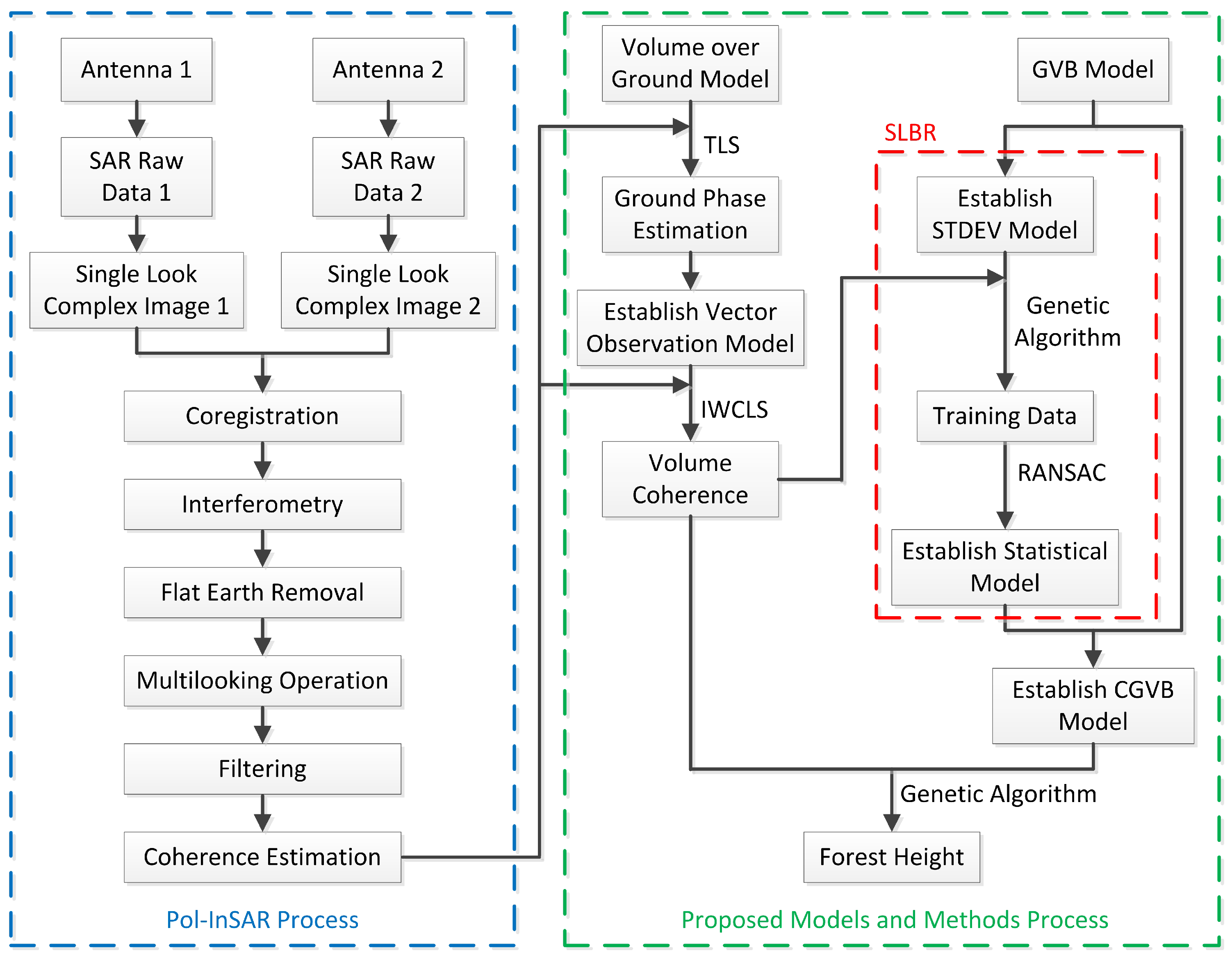
5. Summary of the Proposed Models and Methods

The flowchart of the proposed models and methods is shown in Figure 1. The entire process is divided into two parts. The first part corresponds to the Pol-InSAR data processing consisting of radar echo imaging for two antennas, coregistration, interferometry, flat earth removal, multilooking operation, filtering and coherence estimation, as is revealed in the blue dotted line frame in Figure 1. Most importantly, the proposed models and methods, making up the second part, are the innovation of this paper, divided into three steps. Firstly, based upon volume over ground model, the ground interferometric phase is estimated using the TLS method. Next, the vector observation model is constructed, based on which volume coherence is estimated by IWCLS. Secondly, on the basis of GVB model, the STDEV model is proposed, with which the training data is obtained with genetic algorithm. Using the training data, the statistical model is then constructed and estimated with RANSAC method. Finally, CGVB model is established with the statistical model. Thereby, based on CGVB model the forest height is estimated in virtue of genetic algorithm.

6. Verification of the Proposed CGVB Model and SLBR Method

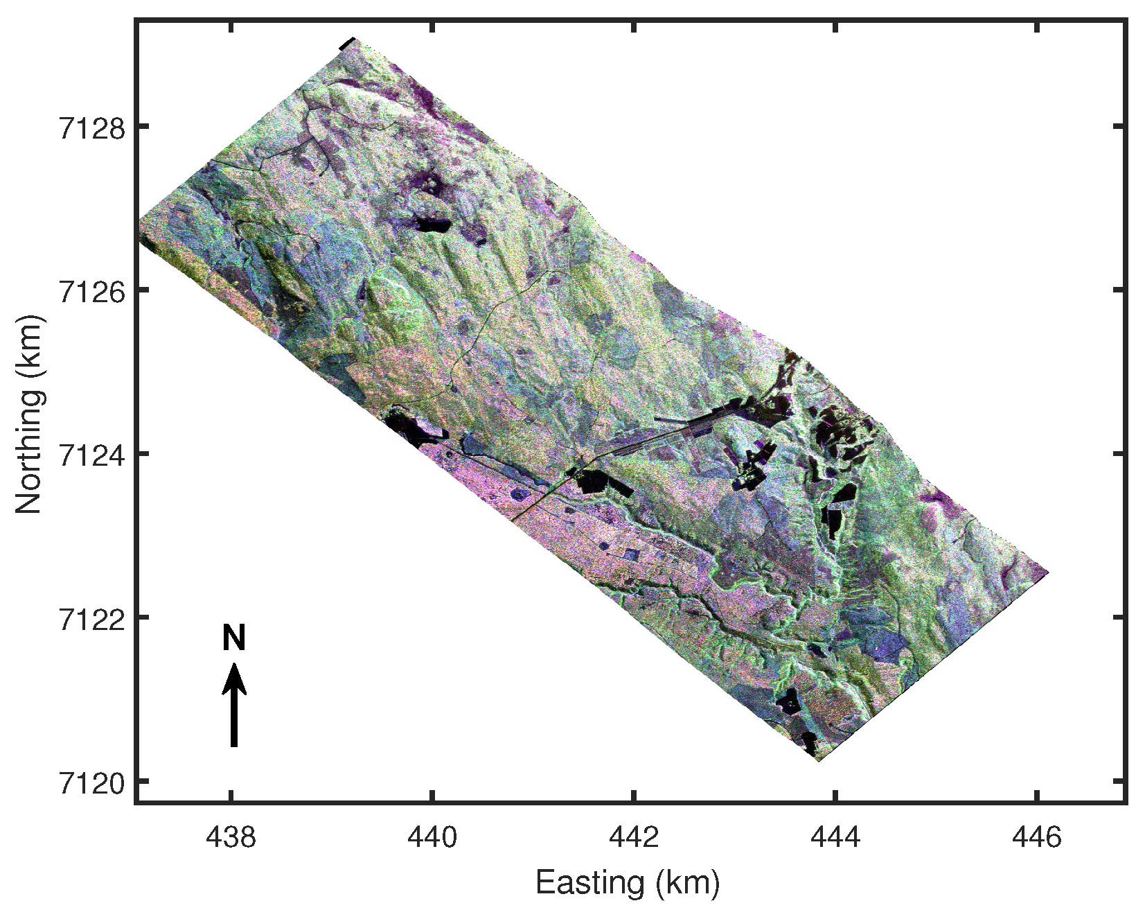
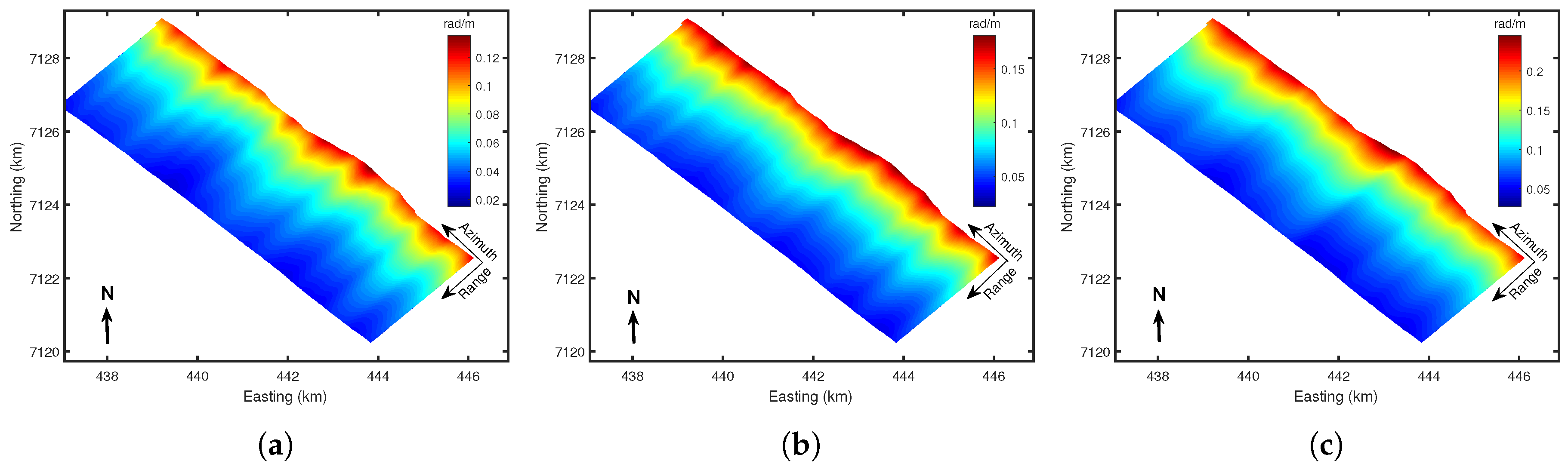
6.1. E-SAR P-Band Pol-InSAR Data

The performance of the proposed CGVB model and SLBR method is evaluated with real airborne repeat-pass E-SAR P-band data. The SAR data was collected in the BIOSAR 2008 campaign by the European Space Agency (ESA) over boreal forest of the Krycklan catchment, Northern Sweden. The Pauli-basis polarimetric composite map of experimental area is shown in Figure 2. The terrain in this area ranges from about 180 to 350 m above the sea level, which can cause conspicuous errors in forest height estimation [28,29,30,31]. Therefore, forest height estimation of this data set requires terrain compensation. The forest height acquired by the lidar is used as true value to evaluate the performance of the proposed CGVB model and SLBR method. Since at least two baselines are required to solve the vector observation model in Equation (8), this paper uses a total of three interferometric pairs, as is shown in

Table 1. Pol-InSAR data used in this paper.

Track	Baseline (m)	${\mathit{k}}_{\mathit{z}}$ Range	Band	Polarization
08biosar0103	Master	Master	P	Quad
08biosar0107	16	0.014–0.135	P	Quad
08biosar0109	24	0.021–0.181	P	Quad
08biosar0111	32	0.026–0.245	P	Quad

. Figure 3 shows the interferometric vertical wavenumbers which correspond to the baselines in Table 1, respectively. Note that the vertical wavenumber here is not corrected by the terrain.

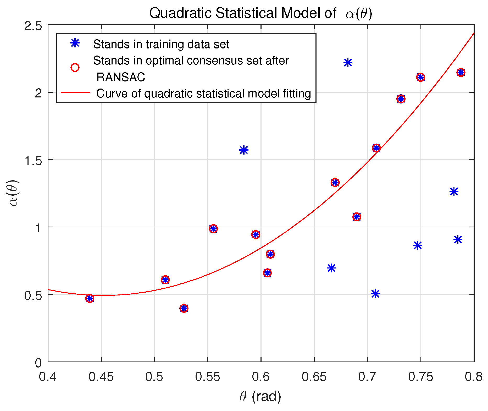
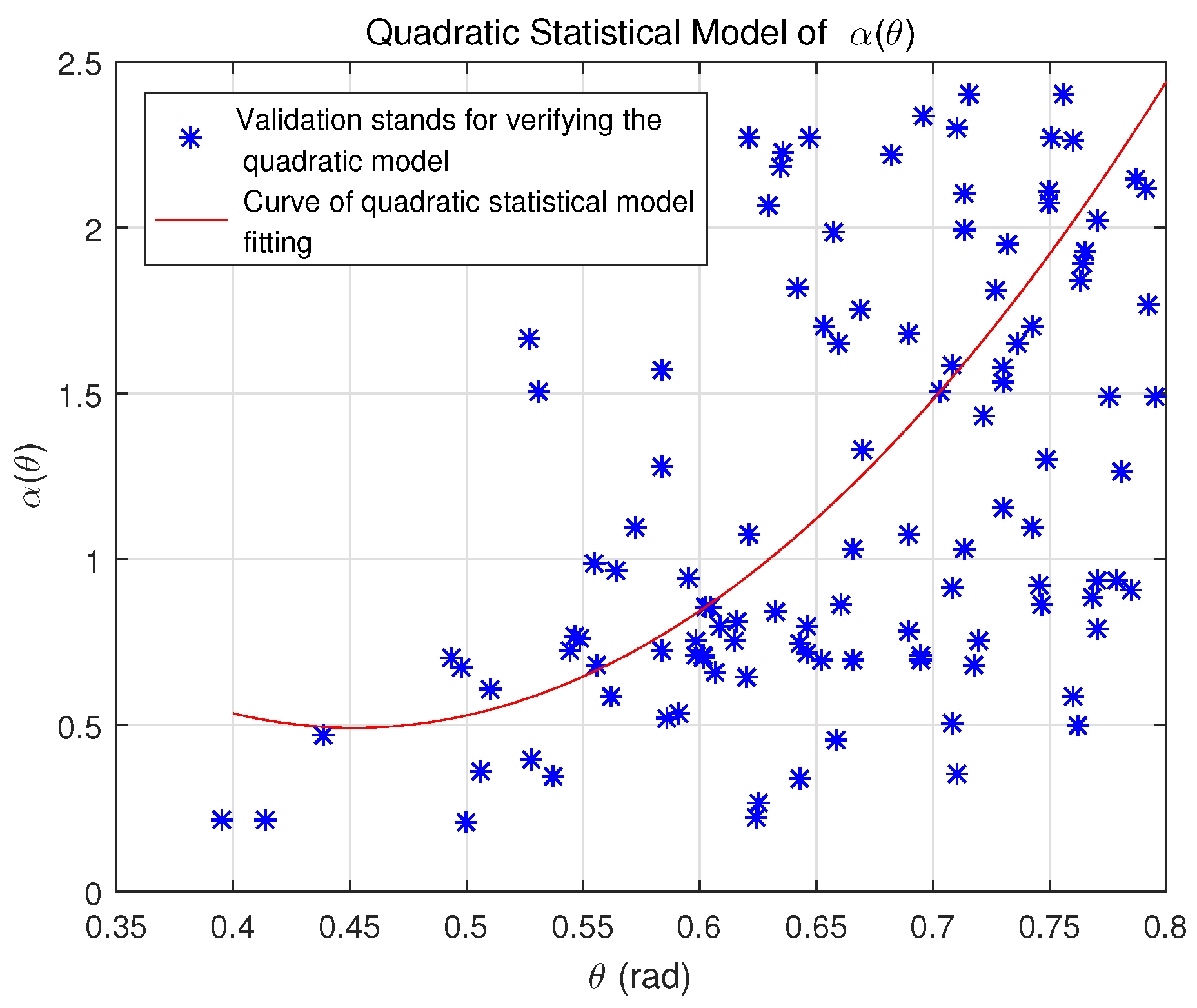
6.2. Establish Quadratic Statistical Model with E-SAR P-Band Pol-InSAR Data

A total of 20 stands (5 × 5 pixels) with uniform forest height were randomly selected to research for the statistical relationship between $\alpha \left(\theta \right)$ and $\theta$ in line with Equation (17). Quadratic function was used to model the curve of training data, and the model parameters were estimated by the RANSAC method. For each selected stand, the LS estimation under the assumption of the quadratic model can be expressed as

$$\begin{array}{c}\hfill {\widehat{\alpha }}_i\left(\theta \right)={\beta }_1{{\theta }_i}^2+{\beta }_2{\theta }_i+{\beta }_3+{\epsilon }_i\end{array}$$

(20)

where ${\beta }_i$ represents the model parameter to be sought and ${\epsilon }_i$ represents noise. Equation (20) is represented by matrix as

$$\begin{array}{c}\widehat{A}=\Theta B+E\hfill \\ {\widehat{A}}_{u\times 1}={\left[{\widehat{\alpha }}_1\left(\theta \right),\dots ,{\widehat{\alpha }}_u\left(\theta \right)\right]}^T\hfill \\ {\Theta }_{u\times 3}=\left[{{\theta }_i}^2,{\theta }_i,1\right]\hfill \\ B_{3\times 1}={\left[{\beta }_1,{\beta }_2,{\beta }_3\right]}^T\hfill \\ E_{u\times 1}={\left[{\epsilon }_1,\dots ,{\epsilon }_u\right]}^T\hfill \end{array}$$

(21)

where u represents the number of stands in the optimal consensus set $S_{opt}^{\ast }$ selected to engage in the model estimation using the RANSAC method. The LS solution of Equation (21) is as follows

$$\begin{array}{c}\hfill \begin{array}{c}\frac{\partial J\left(\widehat{B}\right)}{\partial \widehat{B}}={\left.-2{\Theta }^T\left(\widehat{A}-\Theta \widehat{B}\right)\right|}_{\widehat{B}={\widehat{B}}_{RANSAC}}=0\hfill \\ \Rightarrow {\widehat{B}}_{RANSAC}={\left({\Theta }^T\Theta \right)}^{-1}{\Theta }^T\widehat{A}\hfill \end{array}\end{array}$$

(22)

where $\widehat{B}$ is the estimator of B. ${\widehat{B}}_{RANSAC}$ is the RANSAC estimator of B. $J\left(\widehat{B}\right)$ is the cost function of LS.

Quadratic statistical model was finally established with Equation (22), as is shown in Figure 4. The blue star points indicate the stands in training data set T. The red bubble points represent the stands in the optimal consensus set $S_{opt}^{\ast }$ that was filtered by RANSAC and participated in LS estimation. The red curve represents the statistical model fitting result. Using the statistical model determined by Equation (22), $\alpha \left(\theta \right)$ at each location in the observation area can be obtained. The interferometric coherence of volume layer ${\gamma }_{CGVB}\left(h_v,\delta \right)$ lying exclusively on $h_v$ and $\delta$ in Equation (6) was then determined with $\alpha \left(\theta \right)$, as is shown in Equation (18). Finally, forest height was estimated with Equation (19).

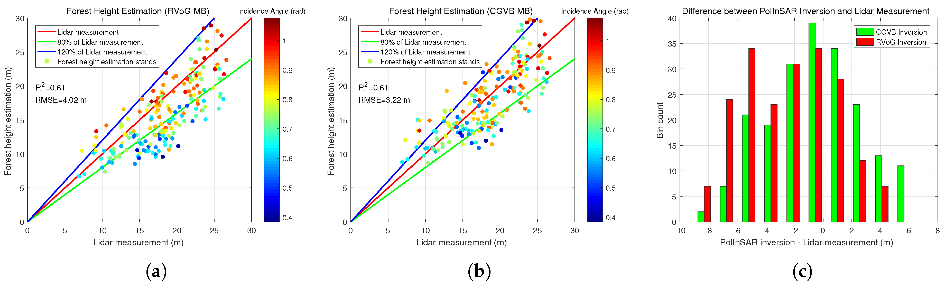
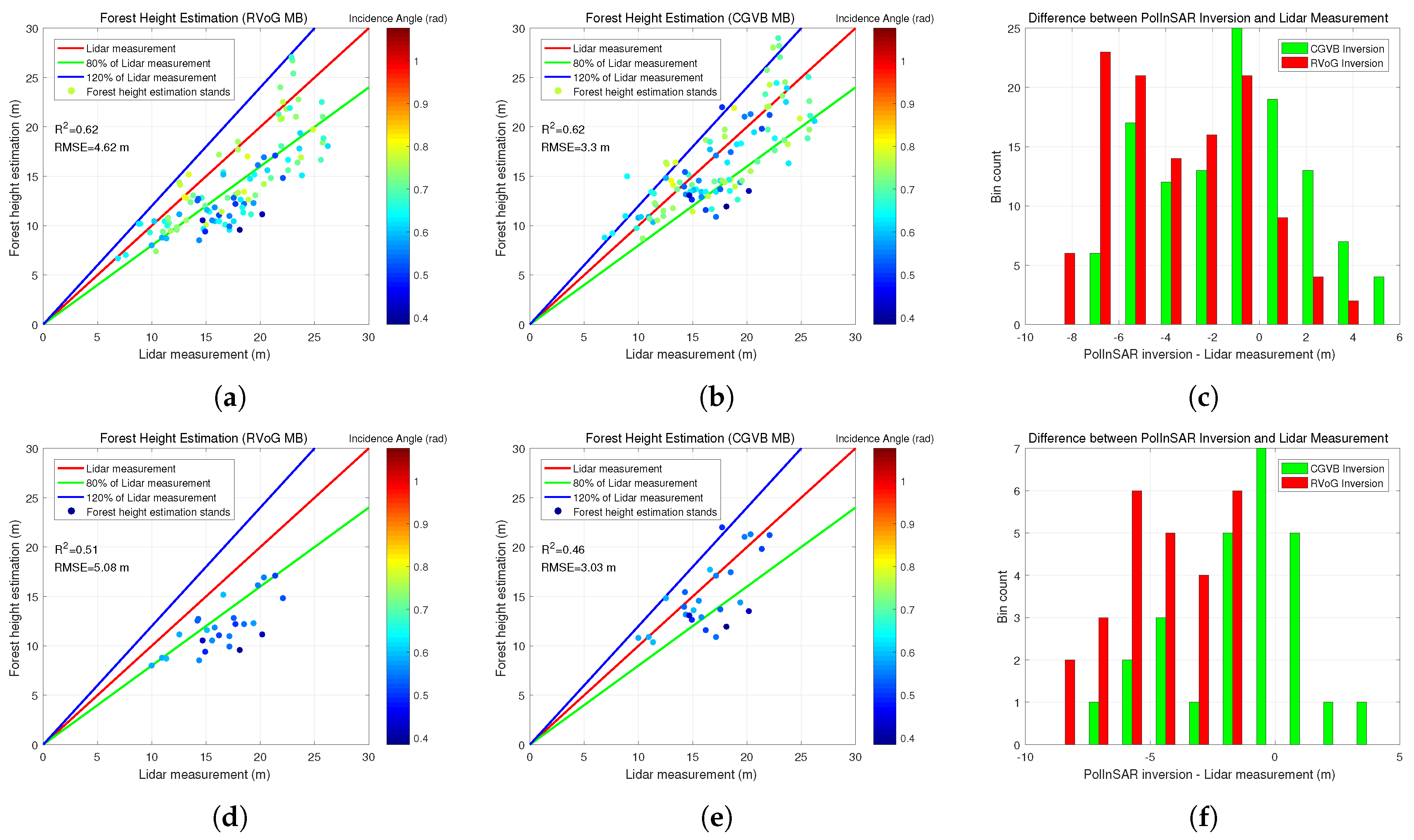
6.3. Forest Height Estimation

As is shown in the flow chart of Figure 1, Pol-InSAR process was carried out to estimate the interferometric coherences of the specified polarization channels for the three baselines presented in Table 1. In order to diminish the influence of temporal decorrelation [32,33] and noise, phase diversity (PD) [34] and magnitude diversity (MD) [10] optimizations were implemented to estimate the canopy-dominated and ground-dominated coherences [21]. That is to say, the interferometric coherences in five polarization channels (PDHigh, PDLow, Opt1, Opt2 and Opt3) were chosen for forest height estimation. In this paper, a window size of 11 × 11 pixels was used to estimate coherences. With the aim of mitigating the effects of observation errors, the time-frequency optimization [20] method was used to preprocess the data before coherence line fitting. The weighting matrix W in Equation (13) is determined by equal weight in this paper to obtain a general conclusion. For fear of obtaining non-physical or local optimal solutions from IWCLS and genetic algorithm, the initial values and constraints of the optimization equation should be circumspectly considered [21]. In this paper, the position relationship of coherences on complex plane [26] were used to determine the initial values and constraints of IWCLS [21]. At the same time, the initial values and constraints of genetic algorithm were set in accordance with the two empirical models introduced in [5,6]. Since each baseline provides five interferometric coherences to calculate the volume coherence, the inversion framework of IWCLS consists of 11 unknowns and 30 equations. Then, the forest height was retrieved in light of the proposed CGVB model and SLBR method, as is shown in Figure 1. In addition, owing to the large terrain fluctuations in the experimental area, this paper used the lidar dem to compensate in the forest height estimation process [28,29,30,31].

In order to compare the performance of RVoG model with the proposed CGVB model, forest height estimation based on each of the two models were obtained, as is shown in Figure 5. Using volume coherence estimated with IWCLS in Section 3 of this paper, forest height estimations on the basis of RVoG and CGVB models are shown in Figure 5a,b, respectively. Since the small incidence angle is not suitable for the RVoG model, the proposed model mainly works on the small incidence angle region, while the large incidence angle region still retains the inversion based on the RVoG model. As can be seen from Figure 5a, the RVoG estimation is significantly underestimated at close range corresponding to smaller incidence angle. However, the CGVB estimation substantially alleviates the underestimation, as is shown in Figure 5b. One noteworthy issue is that the proposed CGVB model overestimates particularly high trees, as is shown in the black circle label in Figure 5b. In order to accurately evaluate the inversion performance of RVoG model and the raised CGVB model, 200 validation stands (10 × 10 pixels) with uniform forest height are randomly selected, and the contrasts between the estimation based on each of the two models and the lidar forest height are shown in Figure 6a,b, respectively. The distributions in Figure 6a,b possess similar correlation coefficients. However, the Root Mean Square Error (RMSE) of Figure 6a is $4.02$ m, while that of Figure 6b is $3.22$ m, $19.9\%$ lower than that of Figure 6a. Note that the CGVB inversion has a certain overestimation in the low forest area. Figure 6c is the histogram of the difference between Pol-InSAR inversion and lidar measurement corresponding to the stands in Figure 6a,b.

Table 2. RMSE varies with forest height.

Lidar Forest Height (m)	$\left(5,10\right]$	$\left(10,15\right]$	$\left(15,20\right]$	$\left(20,25\right]$	$\left(25,30\right]$
Number of stands	10	39	74	62	15
RMSE (RVoG) (m)	2.23	2.72	4.38	4.26	4.8
RMSE (CGVB) (m)	3.85	1.99	3.24	3.57	3.68

shows the relationship between RMSE and lidar forest height. It can be found that in the low forest height range (below 10 m), the inversion based on RVoG model has a better performance, while the advantage of CGVB model is more obvious in the high forest height range (above 10 m). This may be because when P-band is used to observe sparse boreal forest, the shorter forest is no longer suitable for model-based inversion.

As the forest height underestimation based on RVoG model is mainly concentrated in the low incidence angle region, the performance evaluation of the proposed CGVB model is supposed to revolve around this region as well. The forest height estimation of validation stands in the region where the incidence angle is less than $0.8$ rad is shown in Figure 7a,b corresponding to RVoG model and the proposed CGVB model, respectively. The distributions in Figure 7a,b possess similar correlation coefficients. The RMSE of Figure 7a is $4.62$ m, while that of Figure 7b is $3.3$ m, $28.57\%$ lower than that of Figure 7a. Figure 7c is the histogram of the difference between Pol-InSAR inversion and lidar measurement corresponding to the stands in Figure 7a,b. Further focus on the area accords with the smaller incidence angle. The forest height estimation of validation stands in the region where the incidence angle is less than $0.6$ rad is shown in Figure 7d,e corresponding to RVoG model and the proposed CGVB model, respectively. The RMSE of Figure 7d is $5.08$ m, while that of Figure 7e is $3.03$ m, which is $40.35\%$ lower than that of Figure 7d. Figure 7f is the histogram of the difference between Pol-InSAR inversion and lidar measurement corresponding to the stands in Figure 7d,e.

To illustrate the advantages of the GVB or CGVB model over the RVoG model, this paper selected several stands for further study, as is shown in Figure 8. These stands correspond to the CGVB inversion with better performance, while the inversion performance for the RVoG model is poor in Figure 6. Note that the inversion of relative elevation is affected by the constraints in the optimization, so Figure 8 is only a qualitative result. As is illustrated in Figure 8, there is no notable relationship between relative elevation and lidar measurement or incidence angle. However, it can be seen that most of the relative elevations fall into the range less than zero. This means that the relative elevation of strongest backscattered power is located in the lower part of the forest, which is identical to the theoretical analysis of P-band observation. In this case, in virtue of the greater penetration depth [35,36] of the small incidence angle region, the VBP of a small BVF located in this region corresponds to a lower vertical position of power distribution, which is consistent with the expectation of a smaller attenuation in this region. In particular, it should be highlighted that the stands corresponding to the estimated relative elevation below zero indicate that the actual strongest backscattered power is located at the basis of the canopy. It means that the VBP tends to turn into a reversed exponential. That is because the integral limit of the VBP in Equation (2) or Equation (6) is greater than zero. In other words, VBP is meaningless in the part where the vertical coordinate is less than zero. The position relationship between VBP and forest height is illustrated in Figure 9. When the relative elevation is greater than 1, in $(0,1)$, and less than 0, the indications of VBP correspond to (a), (b), and (c) of Figure 9, respectively. Since the RVoG model describes VBP using exponential decay, this case corresponds to (a) in Figure 9. That means the RVoG model fails to describe the VBP in accordance with (b) and (c) in Figure 9, while these two cases can be depicted with GVB model. In other words, RVoG model is described by GVB model when the relative elevation is greater than 1. Owing to the strong penetrability of P-band, VBP is expected to correspond more to the two cases of (b) and (c) in Figure 9. Therefore, GVB model has an edge over RVoG model at P-band.

7. Discussion

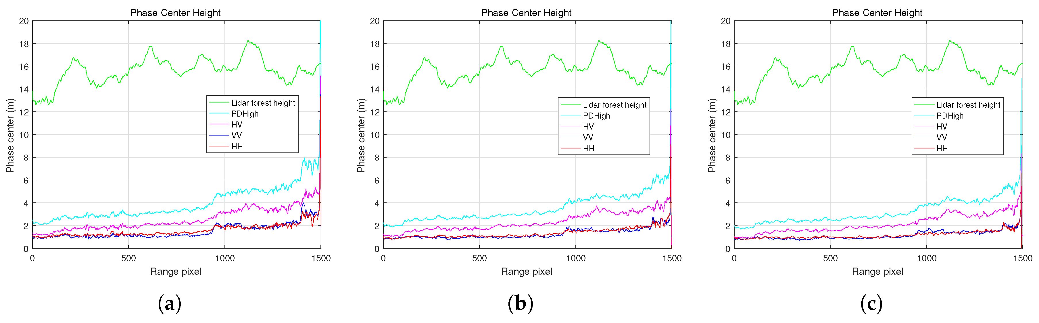
7.1. Phase Center Height of BIOSAR 2008 P-Band Pol-InSAR Data

Since the experimental area of BIOSAR 2008 is covered by sparse boreal forest, there is some aliasing between the phase centers of different polarization channels because of the strong penetration at P-band. It can be seen from Figure 10 that the phase centers of the HH and VV channels are almost completely overlapped. The phase center of the HV channel is slightly higher because it corresponds to the volume scattering of canopy. For the purpose of separating the phase center, PD optimization is implemented to obtain the highest and lowest phase centers. Yet, the phase centers after PD optimization are still close together. This phenomenon is due to the strong penetrability of P-band. Therefore, phase center aliasing will critically affect the effectiveness of the methods which directly take the HV channel as volume scattering for forest height inversion.

7.2. Underestimation Based on RVoG Model

Previous studies upon RVoG model found that the forest height inversion performance using P-band Pol-InSAR data varied with incidence angle [28]. Estimation corresponding to small incidence angle is significantly lower [28,30,37]. According to Equation (3), the vertical wavenumber $k_z$ with small incidence angle is relatively larger due to a large effective baseline [28]. Based on RVoG model, larger vertical wavenumber is not sensitive to forest height inversion using P-band data with strong penetration. On the other hand, a small incidence angle corresponds to a stronger penetration depth, which will lead to a larger error in the inversion based on RVoG model. Therefore, the RVoG model has a significant underestimation in the area correspongding to small incidence angle at P-band. It can be derived from Equation (3) that $k_z$ is relevant to $\theta$ and $\Delta \theta$. Since the change in $\Delta \theta$ with range is exceedingly small when the SAR system parameters are determined, its influence on $k_z$ can be neglected. Therefore, the change trend with range of the inversion performance is basically consistent with that of the incidence angle. Since $\theta$ and $\Delta \theta$ are affected by the system parameters, the value of $k_z$ can be adjusted by SAR system parameters. Thereby, $k_z$ can act within a smaller scope by letting $\theta$ larger or letting $\Delta \theta$ smaller. However, an excessive $\theta$ will cause shadow problem and introduce more noise into the observation data. A smaller $\Delta \theta$ can be achieved by reducing the length of the effective baseline. Yet the reduction of the effective baseline results in a decrease in the accuracy of the elevation measurement. Therefore, in order to reduce noise and increase measurement accuracy, a relatively large $k_z$ is inevitable. In summary, the RVoG model describing homogeneous VBP fails to accurately interpret the heterogeneous VBP under P-band observation, which results in an underestimation of forest height. At the same time, since a small incidence angle corresponds to a stronger penetration depth and the large $k_z$ is not sensitive to the forest height inversion based on RVoG model, especially at P-band, the underestimation phenomenon becomes more serious, resulting in the variation of the inversion performance with the incidence angle. Therefore, this paper uses the GVB model instead of the RVoG model for forest height inversion, considering the influence of incidence angle on the forest model.

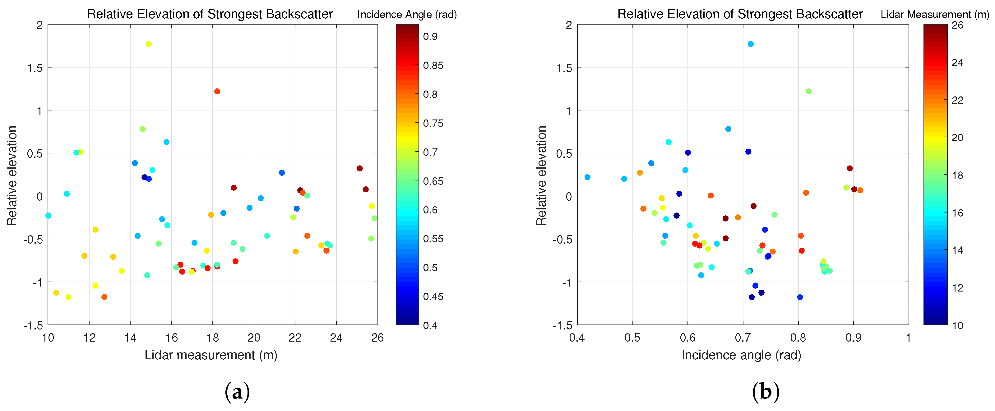
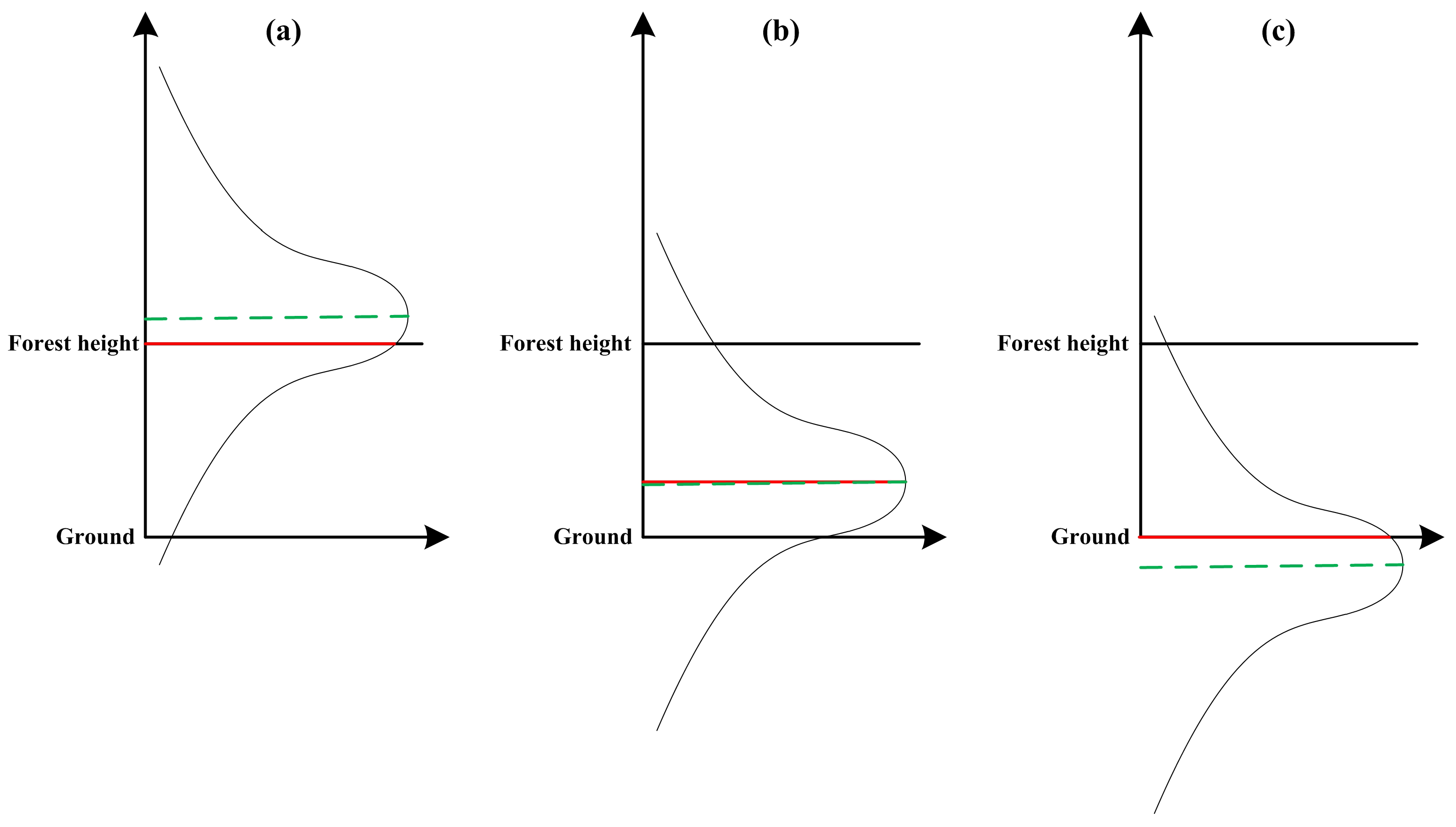
7.3. Influence of Incidence Angle on Vertical Backscatter Profile

To qualitatively evaluate the quadratic model, the optimal $\widehat{\alpha }\left(\theta \right)$ corresponding to 118 validation stands randomly selected in the small incidence angle region are estimated according to Equation (17), as is shown in Figure 11. The red curve is the quadratic statistical model fitting in Figure 4. It can be seen that the model can roughly reflect the correlation between $\alpha \left(\theta \right)$ and $\theta$. Note that the quadratic model is relatively insignificant due to model error, temporal decorrelation, residual noise, as well as a small range of incidence angle variation. In the experiment we found that even when the BVF was fixed to a constant, the underestimation based on RVoG model would be significantly improved. However, when the swath is relatively wide, that is, the incidence angle changes relatively large, it is an unscientific method to approximate the BVF with a constant. Note that a particularly large incidence angle corresponds to a larger $\alpha \left(\theta \right)$, indicating that the power is nearly evenly distributed in the vertical direction. It means that the model has reached a critical state of describing the profile, because a larger $\alpha \left(\theta \right)$ will no longer have any meaning.

7.4. Challenges and Promising Solutions for P-Band Pol-InSAR

For P-band Pol-InSAR, the VBP is heterogeneous and the power distribution is more concentrated in the lower layer of the forest in virtue of the strong penetrability of this frequency. The advantage of this characteristic is that it is capable of getting more abundant information about the vertical structure of the forest. Yet two issues arise out of this characteristic. First, the classic RVoG model describing a homogeneous canopy is a model based on exponential distribution that does not describe the heterogeneous VBP at P-band. Second, for Pol-InSAR at the high-frequency bands, it is generally assumed that there is at least one polarization channel whose GVR is zero. The assumption of NGVR enables the Pol-InSAR inversion (RVoG model) to have unique solution in the case of SB observation. However, since the P-band SAR systems have strong penetrability on the forest area, the assumption of NGVR is no longer valid.

To cope with the first issue, this paper used the GVB model describing heterogeneous VBP instead of the RVoG model to estimate forest height. However, the GVB model is highly complex and has three model parameters. Apart from that, the solution of GVB model is very easy to fall into local optimum. Therefore, this paper applied a prior knowledge of forest height, combined with a linear relationship between forest height and BVF in GVB model [6], to constrain the GVB model in the entire research area with incidence angle, thus reducing the complexity of the GVB model. The new constrained GVB model is called the CGVB model in this paper. Compared with the GVB model with three unknown parameters, CGVB model with only two unknown parameters makes it possible to efficiently extract forest height and structure. Suffice it to say that, it provides an effective alternative model for large-scale forest height extraction. In addition, since CGVB model has only two unknown parameters, it provides a potentiality for SB inversion when some pre-processing methods can be used to obtain accurate volume coherence with SB data, such as [20]. In order to solve the second issue, researchers generally use MB Pol-InSAR data for model inversion. This paper also employed the IWCLS method to estimate volume coherence based on MB data. Comparing with the inversion based on RVoG model, the forest height estimation with IWCLS method applied in this paper is basically consistent with that obtained by previous work [28]. Therefore, IWCLS provides a choice for MB Pol-InSAR model optimization.

7.5. Limitations of the Proposed Models and Methods

Three limitations of the models and methods proposed in this paper also need to be highlighted. Firstly, since the establishment of the vector observation model in Equation (8) requires to use ground phase, the accuracy of the ground phase estimation directly affects the estimation of volume coherence using IWCLS. This paper used TLS method introduced in [26] to fit coherence line and estimate the ground phase. The implementation of TLS method is relatively simple, however, so that it will introduce some errors especially when temporal decorrelation and noise are large. Therefore, some more robust coherence line fitting and ground phase estimation methods are necessary to be adopted, such as the coherence region method [38] and the Maximum Likelihood method [18]. Secondly, in some cases the orientations of crown structure should be considered [20]. Although [6] used ground phases measured over close bare surfaces to see how the extracted VBP varies with polarization, this paper assumes that GVB model is an random volume -based model, to simplify model estimation. Random volume assumes that the attenuation coefficient at different polarization states is the same. However, the hypothesis of random volume is invalid when the canopy structure presents dominant orientations, which means further research is needed to figure out the GVB model considering oriented volume. Finally, this paper only considered forest height as prior information when using the RANSAC method to establish the statistical model. This strategy is very straightforward and simple. When the tree species in the research area is relatively single, such as the BIOSAR 2008 experimental area, which mainly has boreal forests cover, SLBR proposed in this paper is valid. However, when the tree species in the research area is complicated, the STDEV model represented in Equation (5) is not only related to forest height and incidence angle, but also linked to tree species. Consequently, the strategy of establishing the STDEV model and statistical model proposed in this paper is no longer valid. Another factor that can cause errors in STDEV model is forest density. Both tree species and forest density can affect penetration depth which is directly related to BVF. Therefore, when these two factors change relatively large in the research area, the STDEV model cannot be universally applied to the entire research area. One way to solve this problem is to introduce tree species and forest density information into Equation (5) and thereby create the new STDEV model and statistical model. This work will be very meaningful as it will extend the application scope of the models and methods proposed in this paper.

8. Conclusions

With the aim of resolving the problem of heterogeneous VBP under P-band observation, this paper used GVB model to describe the interaction of radar wave with forest structural elements. In addition, to settle the problem that the NGVR hypothesis is invalid under P-band observation, MB optimization was adopted in this paper. The interferometric coherences of the specified polarization channels were estimated with Pol-InSAR process. To establish the vector observation model, the TLS method was employed for coherence line fitting and ground phase estimation. The IWCLS method was employed to estimate volume coherence. A STDEV model depicting the relationship between BVF and forest height was used to simplify the GVB model. Furthermore, considering the effect of the incidence angle on the power decay trend, the incidence angle was introduced into the STDEV model. To determine the influence of the incidence angle on STDEV model, a statistical model based on prior knowledge of forest height was constructed, which was estimated by the RANSAC method. Thereby, with the SLBR method, the CGVB model was established. Finally, according to the CGVB model, forest height was estimated using genetic algorithm from volume coherence.

The proposed CGVB model and SLBR method in this paper effectively alleviate the underestimation of forest height in the close range based on RVoG model. The results with E-SAR data in Figure 6 show that the proposed CGVB model and SLBR method improve the inversion RMSE by $19.9\%$. Besides, Figure 7 demonstrates that the proposed CGVB model and SLBR method improve the inversion RMSE by $28.57\%$ and $40.35\%$ when the incidence angle is less than $0.8$ rad and $0.6$ rad, respectively. Therefore, drawn from real E-SAR data experiments, the conclusion is that the models and methods proposed in this paper provide an effective potentiality for large-scale forest height mapping under P-band observation.

References

1. Treuhaft, R.N.; Madsen, S.N.; Moghaddam, M.; Zyl, J.J.V. Vegetation characteristics and underlying topography from interferometric radar. Radio Sci. 1996, 31, 1449–1485. [Google Scholar] [CrossRef]
2. Treuhaft, R.N.; Siqueira, P.R. Vertical structure of vegetated land surfaces from interferometric and polarimetric radar. Radio Sci. 2000, 35, 141–177. [Google Scholar] [CrossRef] [Green Version]
3. Garestier, F.; Duboisfernandez, P.C.; Guyon, D.; Toan, T.L. Forest biophysical parameter estimation using l- and p-band polarimetric sar data. IEEE Trans. Geosci. Remote Sens. 2009, 47, 3379–3388. [Google Scholar] [CrossRef]
4. Garestier, F.; Toan, T.L. Vegetation modelling for height inversion using insar/pol-insar data. In Proceedings of the IEEE International Geoscience and Remote Sensing Symposium, Barcelona, Spain, 23–27 July 2007; pp. 2322–2325. [Google Scholar]
5. Garestier, F.; Toan, T.L. Forest modeling for height inversion using single-baseline insar/pol-insar data. IEEE Trans. Geosci. Remote Sens. 2010, 48, 1528–1539. [Google Scholar] [CrossRef]
6. Garestier, F.; Toan, T.L. Estimation of the backscatter vertical profile of a pine forest using single baseline p-band (pol-)insar data. IEEE Trans. Geosci. Remote Sens. 2010, 48, 3340–3348. [Google Scholar] [CrossRef]
7. Kugler, F.; Lee, S.K.; Papathanassiou, K.P. Estimation of forest vertical structure parameter by means of multi-baseline pol-insar. In Proceedings of the IEEE International Geoscience and Remote Sensing Symposium, Cape Town, South Africa, 12–17 July 2009; pp. 721–724. [Google Scholar]
8. Cloude, S.R. Polarization coherence tomography. Radio Science 2006, 41, 1–27. [Google Scholar] [CrossRef]
9. Cloude, S.R. Dual-baseline coherence tomography. IEEE Geosci. Remote Sens. Lett. 2007, 4, 127–131. [Google Scholar] [CrossRef]
10. Papathanassiou, K.P.; Cloude, S.R. Single-baseline polarimetric sar interferometry. Geosci. Remote Sens. IEEE Trans. 2001, 39, 2352–2363. [Google Scholar] [CrossRef]
11. Cloude, S.R.; Papathanassiou, K.P. Three-stage inversion process for polarimetric sar interferometry. IEE Proc. Radar Sonar Navig. 2003, 150, 125–134. [Google Scholar] [CrossRef]
12. Roueff, A.; Arnaubec, A.; Dubois-Fernandez, P.C.; Refregier, P. Cramercrao lower bound analysis of vegetation height estimation with random volume over ground model and polarimetric sar interferometry. IEEE Geosci. Remote Sens. Lett. 2011, 8, 1115–1119. [Google Scholar] [CrossRef]
13. Lee, S.K.; Kugler, F.; Hajnsek, I.; Papathanassiou, K. The potential and challenges of polarimetric sar interferometry techniques for forest parameter estimation at p-band. In Proceedings of the European Conference on Synthetic Aperture Radar, Aachen, Germany, 7–10 June 2010; pp. 503–505. [Google Scholar]
14. Kugler, F.; Koudogbo, F.; Gutjahr, K.; Papathanassiou, K. Frequency effects in pol-insar forest height estimation. In Proceedings of the European Conference on Synthetic Aperture Radar, Dresden, Germany, 16–18 May 2006; pp. 1–4. [Google Scholar]
15. Lavalle, M.; Khun, K. Three-baseline insar estimation of forest height. IEEE Geosci. Remote Sens. Lett. 2014, 11, 1737–1741. [Google Scholar] [CrossRef]
16. Neumann, M.; Ferro-Famil, L.; Reigber, A. Estimation of forest structure, ground, and canopy layer characteristics from multibaseline polarimetric interferometric sar data. IEEE Trans. Geosci. Remote Sens. 2010, 48, 1086–1104. [Google Scholar] [CrossRef]
17. Lee, S.K.; Kugler, F.; Papathanassiou, K.; Hajnsek, I. Multibaseline polarimetric sar interferometry forest height inversion approaches. In Proceedings of the ESA POLinSAR Workshop, Frascati, Italy, 19–23 September 2011; pp. 1473–1477. [Google Scholar]
18. Ferro-Famil, L.; Neumann, M.; Huang, Y. Multi-baseline pol-insar statistical techniques for the characterization of distributed media. In Proceedings of the 2009 IEEE International Geoscience and Remote Sensing Symposium, IGARSS, Cape Town, South Africa, 12–17 July 2009; pp. 971–974. [Google Scholar]
19. Treuhaft, R.N.; Cloude, S.R. The structure of oriented vegetation from polarimetric interferometry. IEEE Trans. Geosci. Remote Sens. 1999, 37, 2620–2624. [Google Scholar] [CrossRef]
20. Garestier, F.; Dubois-Fernandez, P.C.; Champion, I. Forest height inversion using high-resolution p-band pol-insar data. IEEE Trans. Geosci. Remote Sens. 2008, 46, 3544–3559. [Google Scholar] [CrossRef]
21. Fu, H.; Wang, C.; Zhu, J.; Xie, Q.; Zhang, B. Estimation of pine forest height and underlying dem using multi-baseline p-band polinsar data. Remote Sens. 2016, 8, 820. [Google Scholar] [CrossRef]
22. Fu, H.Q.; Wang, C.C.; Zhu, J.J.; Xie, Q.H.; Zhao, R. Inversion of vegetation height from polinsar using complex least squares adjustment method. Sci. China Earth Sci. 2015, 58, 1018–1031. [Google Scholar] [CrossRef]
23. Miller, K.S. Complex linear least squares. Siam Rev. 1973, 15, 706–726. [Google Scholar] [CrossRef]
24. Tebaldini, S.; Rocca, F. Multibaseline polarimetric sar tomography of a boreal forest at p- and l-bands. IEEE Trans. Geosci. Remote Sens. 2012, 50, 232–246. [Google Scholar] [CrossRef]
25. Fornaro, G.; Serafino, F.; Soldovieri, F. Three-dimensional focusing with multipass sar data. IEEE Trans. Geosci. Remote Sens. 2003, 41, 507–517. [Google Scholar] [CrossRef]
26. Cloude, S.R. Polarisation: Applications in Remote Sensing; Oxford University Press: New York, NY, USA, 2009. [Google Scholar]
27. Seymour, M.S.; Cumming, I.G. Maximum likelihood estimation for sar interferometry. In Proceedings of the International Geoscience and Remote Sensing Symposium, IGARSS’94, Surface and Atmospheric Remote Sensing: Technologies, Data Analysis and Interpretation, Pasadena, CA, USA, 8–12 August 1994; Volume 4, pp. 2272–2275. [Google Scholar]
28. Hajnsek, I.; Scheiber, R.; Keller, M.; Horn, R.; Lee, S.; Ulander, L.; Gustavsson, A.; Sandberg, G.; Toan, T.L.; Tebaldini, S. Biosar 2008: Final Report. 2009. Available online: https://earth.esa.int/c/document_library/get_file?folderId=21020&name=DLFE-903.pdf (accessed on 21 November 2018).
29. Park, S.E.; Moon, W.M.; Pottier, E. Assessment of scattering mechanism of polarimetric sar signal from mountainous forest areas. IEEE Trans. Geosci. Remote Sens. 2012, 50, 4711–4719. [Google Scholar] [CrossRef]
30. Kugler, F.; Lee, S.K.; Hajnsek, I.; Papathanassiou, K.P. Forest height estimation by means of pol-insar data inversion: The role of the vertical wavenumber. IEEE Trans. Geosci. Remote Sens. 2015, 53, 5294–5311. [Google Scholar] [CrossRef]
31. Xie, Q.; Zhu, J.; Wang, C.; Fu, H.; Lopezsanchez, J.M.; Ballesterberman, J.D. A modified dual-baseline polinsar method for forest height estimation. Remote Sens. 2017, 9, 819. [Google Scholar] [CrossRef]
32. Papathanassiou, K.P.; Cloude, S.R. The effect of temporal decorrelation on the inversion of forest parameters from pol-insar data. In Proceedings of the 2003 IEEE International Geoscience and Remote Sensing Symposium, IGARSS’03, Toulouse, France, 21–25 July 2003; pp. 1429–1431. [Google Scholar]
33. Lavalle, M.; Simard, M.; Hensley, S. A temporal decorrelation model for polarimetric radar interferometers. IEEE Trans. Geosci. Remote Sens. 2012, 50, 2880–2888. [Google Scholar] [CrossRef]
34. Tabb, M.; Orrey, J.; Flymn, T.; Carande, R. Phase diversity: A decomposition for vegetation parameter estimation using polarimetric SAR interferometry. In Proceedings of the EUSAR 2002, Cologne, Germany, 4–6 June 2002; pp. 721–724. [Google Scholar]
35. Managhebi, T.; Maghsoudi, Y.; Zoej, M.J.V. An improved three-stage inversion algorithm in forest height estimation using single-baseline polarimetric sar interferometry data. IEEE Geosci. Remote Sens. Lett. 2018, 15, 887–891. [Google Scholar] [CrossRef]
36. Managhebi, T.; Maghsoudi, Y.; Zoej, M.J.V. Four-Stage Inversion Algorithm for Forest Height Estimation Using Repeat Pass Polarimetric SAR Interferometry Data. Remote Sens. 2018, 10, 1174. [Google Scholar] [CrossRef]
37. Lee, S.K.; Fatoyinbo, T.E.; Lagomasino, D.; Feliciano, E.; Trettin, C. Multibaseline tandem-x mangrove height estimation: The selection of the vertical wavenumber. IEEE J. Sel. Top. Appl. Earth Observ. Remote Sens. 2018, 99, 1–9. [Google Scholar] [CrossRef]
38. Flynn, T.; Tabb, M.; Carande, R. Coherence region shape extraction for vegetation parameter estimation in polarimetric sar interferometry. In Proceedings of the IEEE International Geoscience and Remote Sensing Symposium, IGARSS’02, Valencia, Spain, 22–27 July 2002; Volume 5, pp. 2596–2598. [Google Scholar]
Figure 1. Flowchart of the proposed models and methods.
Remotesensing 11 00042 g001
Figure 2. Pauli-basis polarimetric composite map of experimental area.
Remotesensing 11 00042 g002
Figure 3. Interferometric vertical wavenumber corresponding to baseline lengths of 16 m (a), 24 m (b) and 32 m (c), respectively.
Remotesensing 11 00042 g003
Figure 4. Quadratic statistical model describing the relationship between α ( θ ) and θ .
Remotesensing 11 00042 g004
Figure 5. Forest height estimation with RVoG model (a) and CGVB model (b), respectively.
Remotesensing 11 00042 g005
Figure 6. (a,b): Forest height estimation of validation stands with RVoG model (a) and CGVB model (b), compared with forest height measured by lidar. The color of the dots represents the incidence angle and scales the entire range of incidence angle in the experimental area. (c): Histogram of the difference between PolInSAR inversion and lidar measurement with RVoG model and CGVB model, respectively. The stands that are counted correspond to the stands in (a,b).
Remotesensing 11 00042 g006
Figure 7. (a,b) Forest height estimation of validation stands with RVoG model (a) and CGVB model (b), compared with forest height measured by lidar. The color of the dots represents the incidence angle, scaled from the minimum of incidence angle to 0.8 rad. (c) Histogram of the difference between PolInSAR inversion and lidar measurement with RVoG model and CGVB model, respectively. The stands that are counted correspond to the stands in (a,b). (d,e) Forest height estimation of validation stands with RVoG model (d) and CGVB model (e), compared with forest height measured by lidar. The color of the dots represents the incidence angle, scaled from the minimum of incidence angle to 0.6 rad. (f) Histogram of the difference between PolInSAR inversion and lidar measurement with RVoG model and CGVB model, respectively. The stands that are counted correspond to the stands in (d,e).
Remotesensing 11 00042 g007
Figure 8. Relative elevation of strongest backscatter. Relative elevation is normalized using the lidar measurement. Forest stands correspond to the stands in Figure 6 that satisfy the following two conditions: (1) The inversion error based on the CGVB model is lower than 20 % of lidar measurement; (2) The inversion performance based on CGVB model improves that based on RVoG model by more than 5 % of lidar measurement.
Remotesensing 11 00042 g008
Figure 9. Vertical backscatter profile (VBP) corresponding to three cases: (a) The estimated strongest backscattered power elevation is higher than forest height; (b) The estimated strongest backscattered power elevation is located in canopy; (c) The estimated strongest backscattered power elevation is lower than ground. The green dashed line indicates the estimated strongest backscattered power elevation. The red solid line indicates the actual strongest backscattered power elevation.
Remotesensing 11 00042 g009
Figure 10. Phase center height for different polarization channels, corresponding to baseline lengths of 16 m (a), 24 m (b) and 32 m (c), respectively. The PDLow obtained by phase diversity (PD) optimization is assumed to correspond to ground scattering. The phase centers are processed by averaging along the azimuth direction.
Remotesensing 11 00042 g010
Figure 11. Verification of quadratic statistical model.
Remotesensing 11 00042 g011