Cloud Detection for FY Meteorology Satellite Based on Ensemble Thresholds and Random Forests Approach

Abstract

Cloud detection is the first step for the practical processing of meteorology satellite images, and also determines the accuracy of subsequent applications. For Chinese FY serial satellite, the National Meteorological Satellite Center (NSMC) officially provides the cloud detection products. In practical applications, there still are some misdetection regions. Therefore, this paper proposes a cloud detection method trying to improve NSMC’s products based on ensemble threshold and random forest. The binarization is firstly performed using ten threshold methods of the first infrared band and visible channel of the image, and the binarized images are obtained by the voting strategy. Secondly, the binarized images of the two channels are combined to form an ensemble threshold image. Then the middle part of the ensemble threshold image and the upper and lower margins of NSMC’s cloud detection result are used as the sample collection source data for the random forest. Training samples rely only on source image data at one moment, and then the trained random forest model is applied to images of other times to obtain the final cloud detection results. This method performs well on FY-2G images and can effectively detect incorrect areas of the cloud detection products of the NSMC. The accuracy of the algorithm is evaluated by manually labeled ground truth using different methods and objective evaluation indices including Probability of Detection (POD), False Alarm Rate (FAR), Critical Success Index (CSI) and the average and standard deviation of all indices. The accuracy results show that the proposed method performs better than the other methods with less incorrect detection regions. Though the proposed approach is simple enough, it is a useful attempt to improve the cloud detection result, and there is plenty of room for further improvement.

1. Introduction

According to the global cloud data provided by the International Satellite Cloud Climate Program, clouds cover more than 60% of the earth’s surface [1]. Therefore, remote sensing observations inevitably require cloud detection. For the resource remote sensing, the satellite image is blocked by the cloud during the imaging process. This results in the spectral distortion of the original object, which affects the mapping product and image interpretation, and has a great influence on information extraction. Therefore, the cloud detection before remote sensing image processing has important practical significance [2,3]. While for the meteorology research, cloud itself is the observation object since many meteorological process and weather events are reflected on the behavior of clouds. Hence, the first process step of meteorological satellite images is cloud detection, and the accuracy of cloud detection directly determine the accuracy of meteorological parameter extraction.

FY serial meteorological satellites have made great contributions to meteorology, oceanography, agriculture, forestry, water conservancy, aviation, navigation, and environmental protection [4,5,6]. Cloud detection and quantitative discriminant and its computer implementation in the meteorological satellite cloud map are the main tasks of meteorological satellite cloud map information processing. There are many researches focusing on cloud detection of other meteorological satellites [7], however, for FY satellites, the most authoritative results are from National Satellite Meteorological Centre (NSMC). In practical applications, we found that the officially provided cloud products may have more detection and misdetection in some regions; therefore, it is necessary to try to improve the cloud detection performance in these regions.

There are many cloud detection methods for resource satellites, but accurate cloud detection is still an easily overlooked aspect of remote sensing processing and analysis [2,3,8]. The existing algorithms based on image processing mainly use the characteristics of the spectrum [4,9,10,11,12], frequency [10], texture of the cloud [2,13,14], threshold method [15,16,17,18,19], support vector machine method [20,21], and clustering method to perform detection [22]. The spectral and threshold combination method mainly utilizes the characteristics of what the cloud strongly reflects on the visible band, but these types of methods are highly sensitive to the threshold. The detection threshold for the same satellite data will change greatly due to time and weather, which increases the limitations of these methods [23,24]. The frequency combined threshold method mainly uses the low-frequency characteristics of the cloud and obtains the low-frequency information of the image through wavelet analysis, Fourier transform, etc. to perform cloud detection. However, due to ground-based low-frequency information interference, multi-layer wavelet transform is usually used to eliminate this interference, which greatly reduces the efficiency of cloud detection [25,26,27]. The texture feature-based method utilizes differences between cloud and ground texture features, often using sub-block sub-graphs as the unit, combining second-order moments, fractal dimensions, gray-level co-occurrence matrix, and multiple bilateral filters to calculate texture features. This type of method needs to obtain reliable cloud feature intervals in advance to ensure the accuracy of classification and low efficiency [2]. Support vector machine and clustering method need to acquire many training samples, which requires high selection of classification features, and needs to re-select samples for different data, resulting in the low efficiency [2,18,20,21,28].

In recent years, machine learning has achieved great success in ecology, medicine, remote sensing, transportation and other fields [3,29,30,31,32,33]. In the context of remote sensing image data, through the training of remote sensing images, it is possible to explore the potential complex and rich information of the image through machine learning ideas [34,35]. This paper proposes a cloud detection method based on ensemble threshold method and random forest (RF) algorithm for FY-2G satellite imagery. This method first proposes an ensemble threshold method to perform preliminary cloud detection on remote sensing images. The obtained results are integrated with the NSMC FY-2G product to obtain RF training samples. Secondly, the RF algorithm is used to train the samples to obtain the model, and then the test samples of the original FY-2G images are tested using the trained RF model. Finally, the results of the proposed method are compared with officially provided products by subjective and objective indices.

The remainder of this manuscript is organized as follows. Section 2 describes the official procedure of cloud detection products. The proposed methodology for cloud detection is introduced in Section 3 including the ensemble threshold method and RF-based approach, followed by the cloud detection experiments and results in Section 4. Further discussions and conclusions are arranged in Section 5 where we give a brief summary of our works.

2. Materials and Methods

2.1. NSMC Cloud Detection

The information of FY-2G remote sensing images from the National Satellite Meteorological Center in the format HDF5 is shown in

Table 1. bands information of FY-2G.

Band	Wavelength	Band Name	Spatial Resolution
1	0.55–0.9 µm	Visible (VIS)	1.25 km
2	10.3–11.3 µm	Thermal infrared (IR1)	5 km
3	11.5–12.5 µm	Thermal infrared (IR2)	5 km
4	6.3–7.6 µm	Water vapor (IR3)	5 km
5	3.5–4.0 µm	Mid-infrared (IR4)	5 km

. The image consists of five bands:

The NSMC has developed an operational cloud detection system for FY serial images which can be divided into the following steps.

• Dividing the images into blocks and calculating the mean and variance of the large pixels. For each block, taking the mean value of large pixels as the abscissa and the variance of large pixels as the ordinate, the block structure can be obtained as shown in the following figure (Figure 1).
• For each block, finding the parameters of the parabola model and removing the pixels outside the parabola.

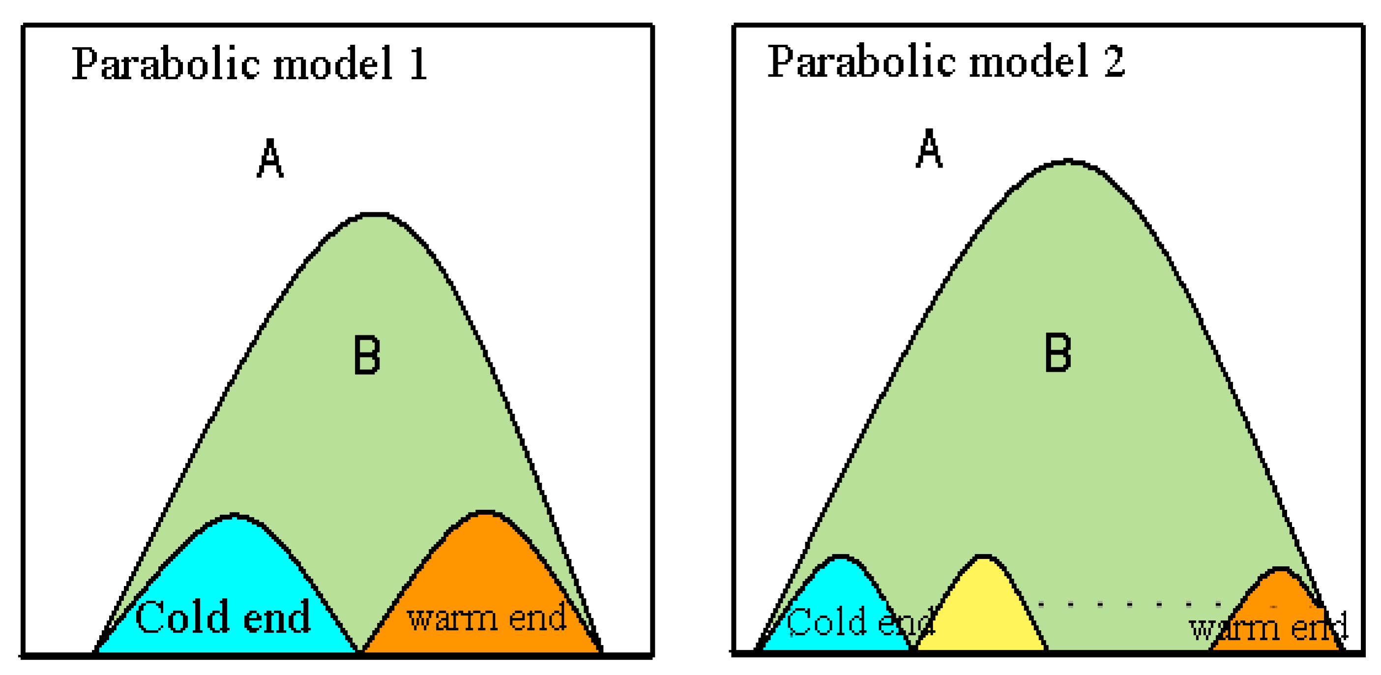
The pixels outside the parabola of Figure 2 (A-zone) are the mixed pixels of the cold and warm ends, which are generally located at the boundary of the two clouds. For the interior of the parabola, except for the cold end and the warm end, there should also be some categories. Each category also has a cold end and a warm end. The same parabolic equation is used to get the parabolic structures of all intermediate categories. It is possible to get the pixels contained in each category.

3.

Extracting uniform pixels. The analysis shows that the variance behavior of large pixels reflects the uniformity of pixel distribution. In the histogram of variance of large pixels, the small part of the variance accounts for a large proportion and becomes larger within a block. A maximum peak could be found from the histogram of the pixel-variance, and the valley on the right side of the peak is used as the threshold. If the number of pixels obtained is greater than 5% of the total number of pixels in the block, this threshold is used as the uniform cell threshold. The number of pixels is accumulated from the minimum value on the histogram until the number of obtained pixels exceeds 5% of the total number of pixels as a threshold. The pixels in the block can be obtained based on the obtained threshold.

4.

The uniform pixel can be analyzed using the histogram and water vapor infrared band. Firstly, the histogram of water vapor band is analyzed to get the corresponding category, and then the histogram of infrared band is used for each category for further classification, thus the uniform pixels can be divided into multiple categories. Histogram analysis involves histogram smoothing, automatic identification of peaks and valleys, and fault-tolerant processing.

5.

Using the minimum distance method to classify the remaining pixels into the corresponding categories.

6.

According to the slope of the infrared-water vapor scatter, the obtained categories are identified as specific clouds.

7.

Since segmentation according to a segment area may cause discontinuity of cloud types between two adjacent segments, a re-matching process between segments is finally required.

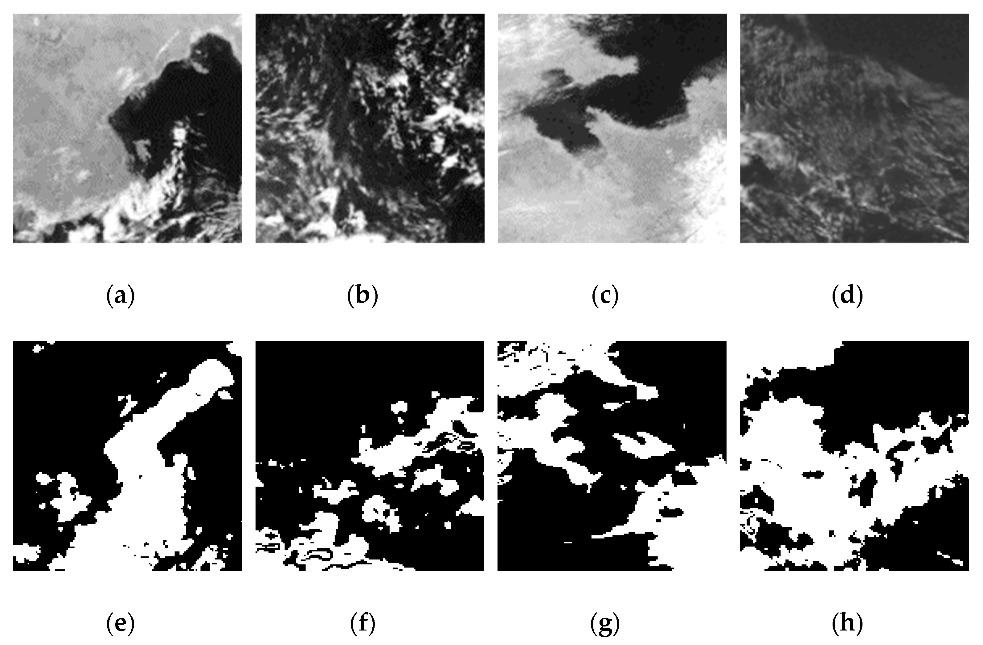
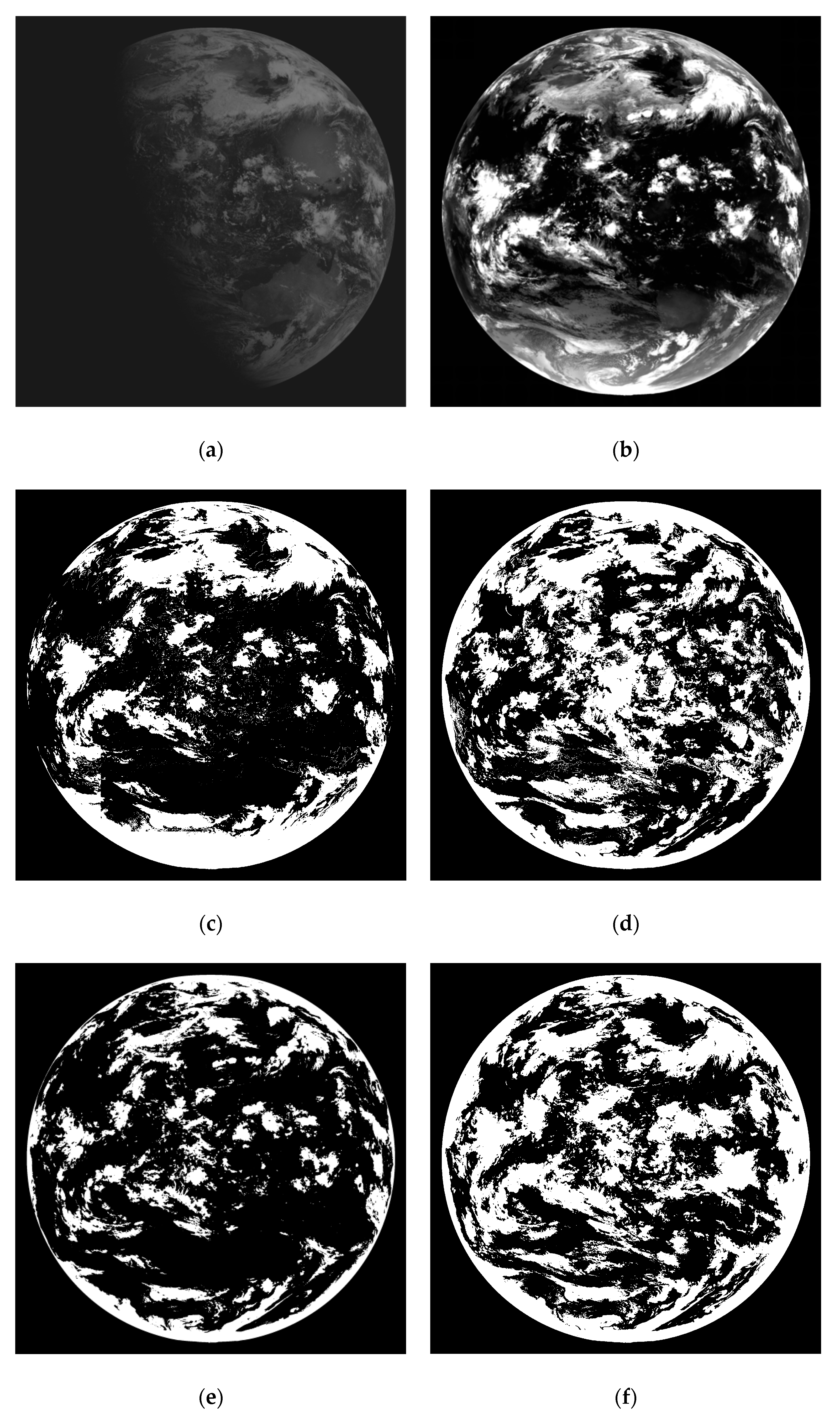
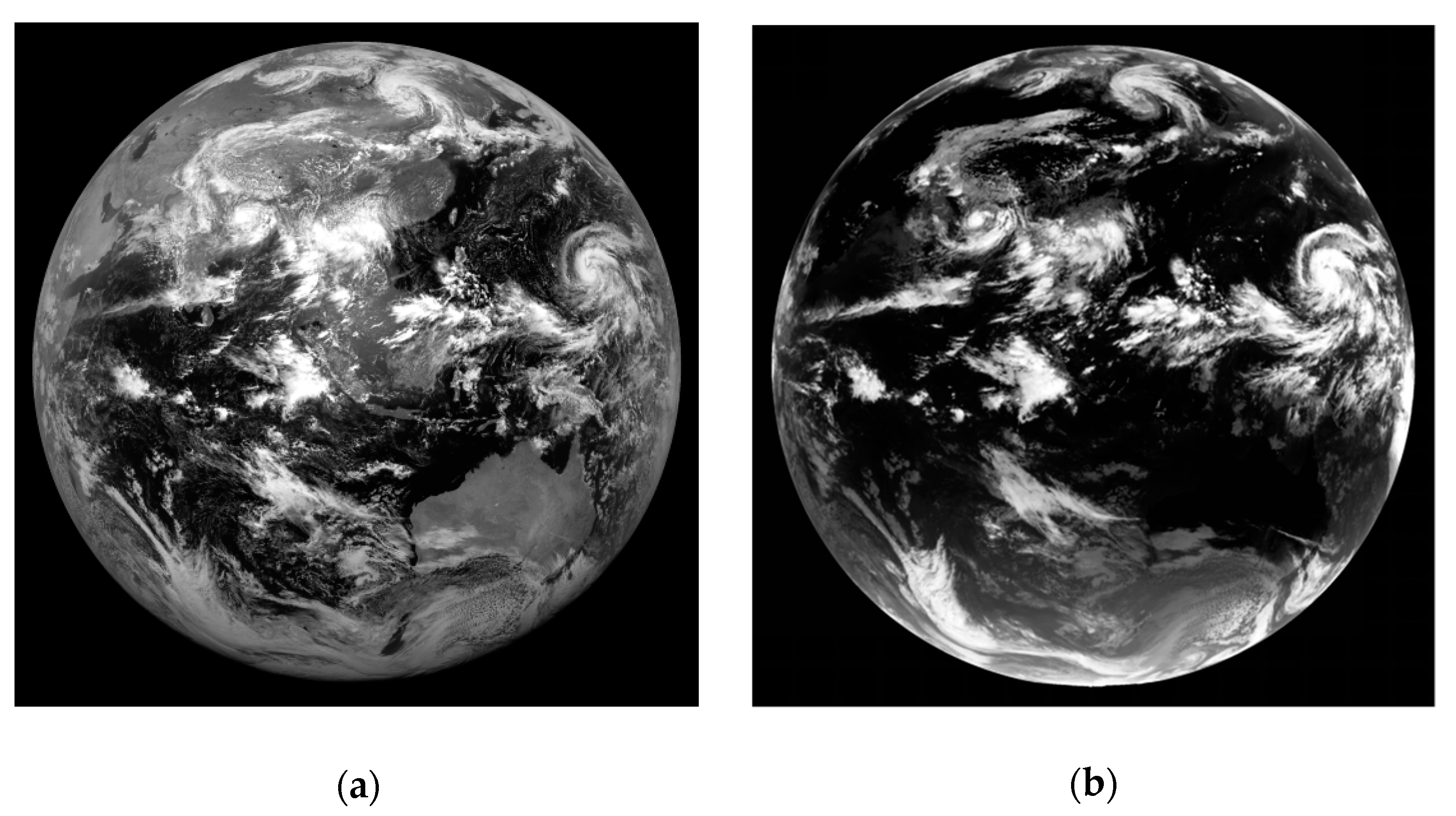
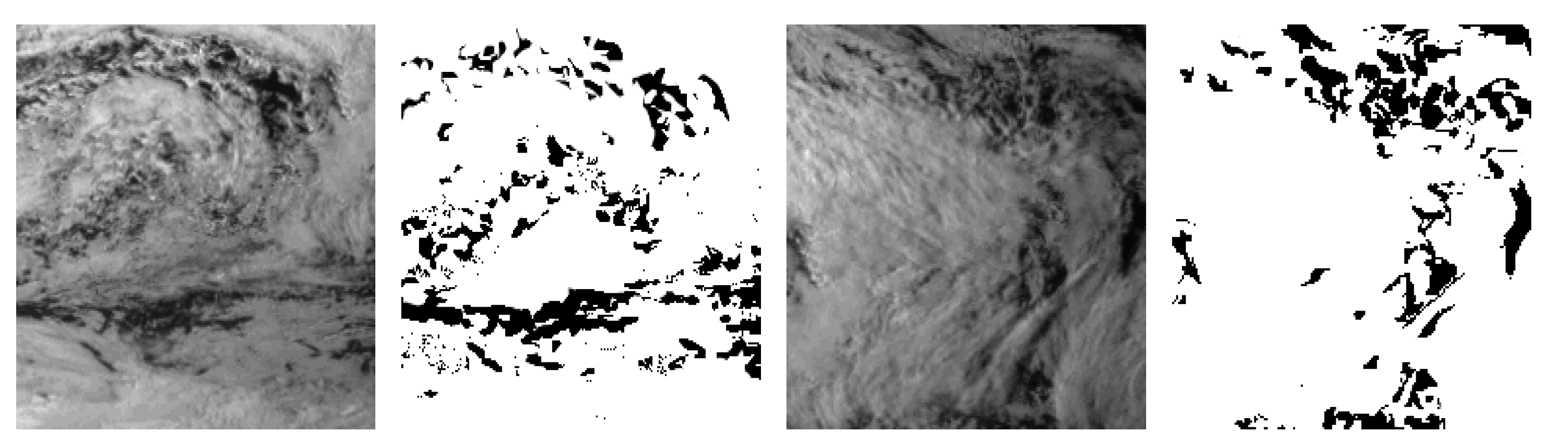
In most cases, the NSMC’s cloud products show good accuracy, however in some areas, there still exists more detections and misdetections in some regions as shown in Figure 3. The Figure 3a–d are the original images, and the Figure 3e–h are the corresponding cloud detection results. It is obvious that there are many misdetections. Therefore, this paper aims to improve the NSMC cloud detection product. This method firstly uses the ensemble thresholds approach to perform preliminary cloud detection on FY-2G remote sensing image, and then selects the training and testing samples for random forest technology from the preliminary result combined with NSMC result to obtain the final cloud detection results. This paper provides a simple way to make full use of the FY-2G satellite cloud classification results of the NSMC.

2.2. Random Forest Algorithm

The RF algorithm is an ensemble learning strategy based on the divide-and-conquer idea and a multi-classifier model for the Categorical and Regression Tree (CART) decision tree. RF consists of many decision trees. Each tree depends on a random vector, and all vectors are independent and identically distributed. Each tree is independently classified to obtain its own classification result, and the final result is voted according to the classification result of each tree.

In the RF algorithm, parameters m and n need to be defined first, where n represents the number of decision trees and m denotes the number of attribute features on each node. Firstly, n samples are extracted from the original training sample set, and the remaining data are used to estimate the classification error. Then, each sample set is used as a training set to generate a single decision tree. At each node of the tree, m feature variables are randomly selected from the feature variables as predictors, and an optimal feature variable is selected for classification. RF uses the CART algorithm to generate a decision tree. In the CART algorithm, each node selects the optimal splitting tree according to the GINI index. For a given training set, the GINI index formula is as follows:

$$GINI={\displaystyle \sum {\displaystyle \sum _{i\ne j}[f(C_{i}T)/|T|][f(C_{j}T)/|T|]}}$$

(1)

where T is the number of learner sets $\{h_1,h_2,\dots ,h_T\}$, $f(C_{i}T)/\left|T\right|$ is the probability that the selected class belongs to $C$.

The GINI index can measure the differences between classes. When the GINI index increases, the differences between classes increase and vice versa. If the GINI index of the child node is smaller than the parent node, then the node is split. When the GINI index is 0, the division is terminated, and one class is separated. When decision trees generate forests, the prediction results of these decision trees are used to predict new data sets. For classification procedure, learner $h_i$ predicts a class from class set $(c_1,c_2,\dots ,c_N)$. The most common classification method is voting. The predicted output of $h_i$ on the test sample could be denoted as an N-dimensional vector $(h_i^1(x),h_i^2(x),\dots ,h_i^N(x))$, and then the formula for majority voting methods is as follows:

$$H(x)=\{\begin{array}{l}{c}_{j}f{\displaystyle \sum _{i=1}^T{h}_i^j(x)>0.5{\displaystyle \sum _{k=1}^N{\displaystyle \sum _{i=1}^T{h}_i^k(x)}}}\\ rejectotherwise\end{array}$$

(2)

where $h_i^j$ is the output of $h_i$ in the class $c_j$. If a class gets more than half of the votes, then the prediction result is this class, otherwise the prediction is rejected.

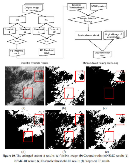
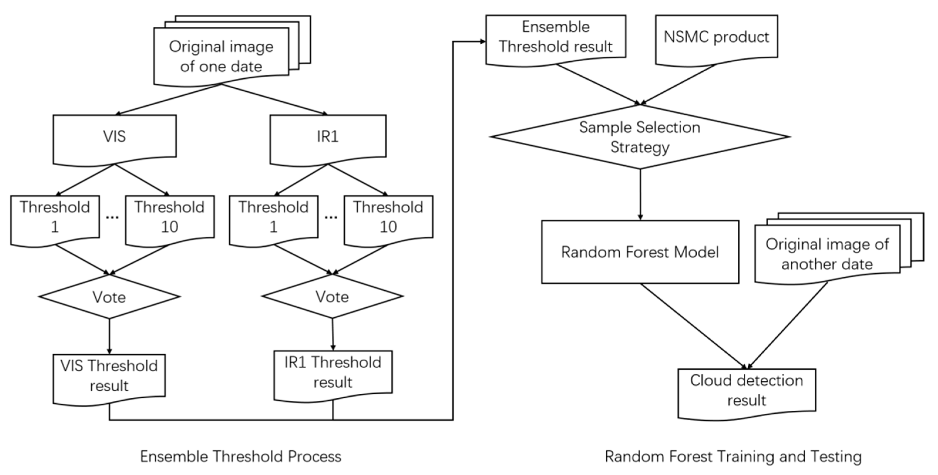
2.3. The Overall Flow Chart of the Proposed Method

The experiment requires the IR1 and visible bands of the source image for ensemble threshold method. Firstly, the IR1 image and visible image are binarized using various threshold methods respectively. Then the obtained binarized images are voted to get threshold images respectively. The IR1 threshold image and visible threshold image are combined to obtain the ensemble threshold image. Due to the fact that the middle part of the ensemble threshold image has good detection, but the marginal parts have poor detection, the marginal parts of the NSMC cloud detection are well performed but the middle part is partially misdetection. The method proposed in this paper tries to take full advantage of the ensemble threshold detection and NSMC’s cloud detection. For the training step, the upper and lower 1/4 part of NSMC result and the middle part of ensemble threshold result forms a cloud detection image R. The training samples are selected from this image R and the corresponding five-band source image. The trained model is then used on the other images obtained on other date, i.e., the training processing is performed on a source image of one date and the testing is on the other date. The following flow figure (Figure 4) illustrates the main steps of the proposed method.

2.4. Various Threshold Methods

2.4.1. OTSU

The OTSU algorithm, also known as the largest inter-class difference method, was proposed by OTSU in 1979. This method is simple to calculate and is not affected by the brightness and contrast of images. It divides the image into two parts, the background and the foreground, according to the gray characteristic of the image. The grayscale average of foreground, the probability of foreground pixels to the total pixels, the grayscale average of background, the probability of the background pixels to the total pixels, the mean and variance of the image are obtained. Since the variance is a measure of the uniformity of the gray distribution, the greater the variance between the background and the foreground, the greater the difference between the two parts that make up the image. When the foreground pixels are misclassified into the background or the background pixels are misclassified into the foreground, the difference between the two parts will become smaller. Therefore, the segmentation that maximizes the variance between classes means that the probability of wrong division is the smallest.

2.4.2. Block OTSU Method

The block OTSU method divides the image into different blocks of the same size, and then uses the OTSU threshold method for each block. Therefore, the blocked OTSU method could better preserve the local features and make the details more visible.

2.4.3. Local Dynamic Threshold Method

The threshold for each pixel is not fixed but is determined by the distribution of neighboring pixels around it. The threshold of the image region with higher luminance is usually bigger, and the threshold of the image region with lower luminance is smaller. Local image regions with different brightness, contrast, and texture will have corresponding local thresholds.

2.4.4. Combining Global Thresholds with Local Thresholds

Firstly, an initial estimated value T (average gray-scale of the image) is selected for the global threshold, and the image is binarized by T. The segmentation result consists of two types of pixels: G1 is composed of pixels having a gray value greater than T, and G2 is composed of pixels less than T. After calculating the average values m1 and m2 of G1, G2 respectively, the new threshold is (m1 + m2)/2, and the previous steps are repeated until the difference between the two T values in consecutive iterations is zero. Local thresholds are obtained using the similar approach. Better binarization results could be obtained by combining the local and global thresholds.

2.4.5. Weller Adaptive Threshold

Assuming that each line of the image is a row vector, the Weller adaptive threshold method first goes through the image and calculates a moving average for each pixel. If the value of a pixel is significantly smaller than this average, this pixel is set to black, otherwise it is set to white.

Suppose $p_n$ is the pixel at point $n$ in the image, $f_s(n)$ is the sum of the last s pixels at point n, and the final image $T(n)$ is 1 (white) or 0 (black), depending on whether it is darker than t% of the average of its first s pixels. The formula is as follows:

$$T(n)=\{\begin{array}{l}1if{p}_n<(\frac{f_s(n)}{s})(\frac{100-t}{100})\\ 0otherwise\end{array}$$

(3)

2.4.6. Minimum Error Method

The assumption of the minimum error method is that the gray-scale image consists of target and background, and the target and the background satisfy a mixed Gaussian distribution. The mean and variance of the target and the background are calculated, and the objective function is the minimum classification error. The minimum threshold is the optimal threshold. Finally, the image is transformed to binary images using this optimal threshold.

2.4.7. Bimodal Method

The bimodal method is a simple segmentation algorithm which is based on the threshold obtained by the double peak method. There are two peak-like histogram distributions. The two peaks are Hmax1 and Hmax2. Their corresponding gray values are T1 and T2, respectively. The idea of bimodal image segmentation is to find the lowest value of the valley between the two peaks of the histogram, that is, to find the threshold $T_h$ within the gray range of [T1, T2] where the number of corresponding pixels is minimum, and the image is segmented with $T_h$.

2.4.8. Iterative Threshold Method

The algorithm of the iterative image binarization is that, first, a threshold $T_h$ is initialized, and then this threshold is continuously updated by iteration according to a certain strategy until a given constraint condition is satisfied. The basic steps are as follows: for an image, assuming that the current pixel is $f(x,y)$ and a threshold $T_h$, according to the current threshold, the image is divided into two sets of pixel sets: A, B; then the averages of A and B sets are calculated as ${\mu }_A$ and ${\mu }_B$, and the updated threshold $T_h$ is the mean value of ${\mu }_A$ and ${\mu }_B$. Finally, the current threshold and the last calculated threshold are determined whether their difference satisfies the constraint condition. If it is less than the current threshold $T_h$, then the optimal threshold is obtained; otherwise, the averages of A and B sets are calculated as ${\mu }_A$ and ${\mu }_B$, and the previous steps are repeated.

2.4.9. Maximum Entropy Threshold Method

The maximum entropy-based image segmentation method uses the gray distribution density function of the image to define the information entropy of an image. By optimizing a certain entropy criterion to obtain the threshold corresponding to the maximum entropy, the image segmentation threshold is obtained. Firstly, for a gray-scale image with the gray-scale range [0, L−1], the minimum gray-scale level is min and the maximum gray-scale level is max. Secondly, according to the formula of entropy, the entropy $E(t)$ corresponding to gray t is obtained. Finally, the entropy value $E(t)$ corresponding to different gray levels $t$ from the minimum gray level min to the maximum gray level max is calculated to obtain the gray level $t$ corresponding to the maximum entropy, which is the desired threshold value $T_h$.

2.4.10. Fixed Threshold Segmentation

Fixed threshold segmentation means artificially setting a threshold value $T_h$. The threshold value needs to be empirically determined. The threshold value directly affects the quality of the binarization result. Therefore, when setting the threshold value, the previous thresholds from the above mentioned nine methods are calculated and the average threshold is set to be a fixed threshold. When the gray value of current pixel is smaller than this threshold, the pixel is set to be 0, otherwise it is set to be 1.

2.5. Ensemble Threshold Cloud Detection Method

The ensemble threshold cloud detection method is based on multiple threshold segmentation algorithms. The main idea is that the results obtained by the single threshold segmentation method may be inaccurate, while the cloud detection results obtained by ensemble multiple threshold segmentation images through a combination strategy can lead to a better result.

In the process of ensemble threshold cloud detection, the parameter that affects the final detection is the voting coefficient $\delta$ which determines the degree of the combination strategy. This paper uses the results of a series of threshold detections described above to apply the ensemble threshold cloud detection. According to various threshold segmentation methods, the cloud detection results are $(F_1,F_2,\dots ,F_p)$, where $F_p$ is the cloud detection result corresponding to the p-th threshold segmentation method. In order to find the best δ value, we use the $\delta$ sequence $({\delta }_i,{\delta }_2,\dots ,{\delta }_i)$ as the voting coefficient to vote for multiple threshold cloud detection results and obtain the ensemble results $(F_{{\delta }_1},F_{{\delta }_2},\dots ,F_{{\delta }_i})$. Some subareas with manually labeled clouds are used to determine the accuracy of ensemble results, and $\delta$ value according to the highest accuracy is the final voting coefficient. The final ensemble result is the one using the final voting coefficient. In our experiments, we find that the voting coefficient setting as 7 would lead to the best ensemble result, that means, if there are more than 7 threshold method indicating a pixel as cloud, it is the cloud. It should be noted that the voting coefficient 7 is an empirical parameter; maybe another value would be better for other experiments.

2.6. Random Forest Method Based on Ensemble Threshold and NSMC Cloud Detection

2.6.1. Training Samples Selection

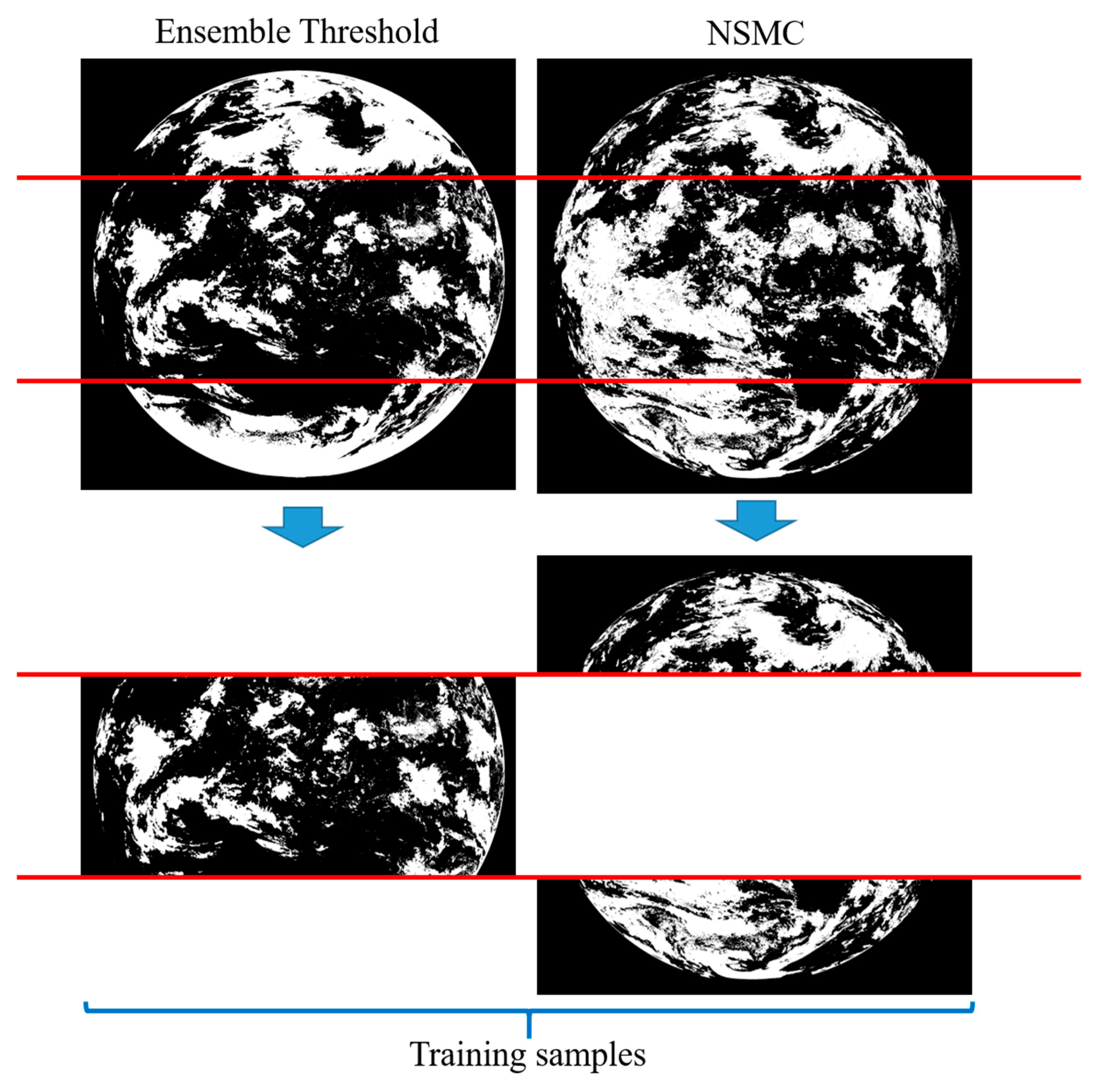
For the FY-2G satellite cloud detection, the NSMC results perform well at the marginal areas, especially at the top and bottom of the image, but there are partial misdetections at the local central part, such as mistakenly detecting part of the water or land as clouds. However, the cloud detection results based on the ensemble threshold method performed well in the middle part of the images, but misdetections exist in the marginal detection. Therefore, in order to ensure the accuracy of the cloud detection, we use the 1/4 of the upper and lower parts of the NSMC cloud detection results and the middle 1/2 part of the ensemble threshold cloud detection results as the training data. Since the random forest training model has good portability, this paper only uses the source image data of one moment to choose the training samples, and then uses the sample to conduct random forest training to get the corresponding model, which is used to perform cloud detection on images acquired on other dates or other moments. Figure 5 illustrates the sample selection procedure.

A certain number of representative pixels are randomly selected from the source image at one moment to form a total training sample set. The boot-strap resampling method is used to generate a training set, i.e., a new training set is formed by extracting N times in a put-back manner from the total training set. Secondly, the appropriate features are selected as the classification attributes. Then, the RF uses each training set to generate a corresponding decision tree for classification. Finally, the test sample sets are obtained from other date/time images, and each test tree is used to classify the test samples. Using the voting strategy in Section 3.3, the category with the most output of the RF is taken as the class which the test sample belongs to.

2.6.2. Parameters of Random Forest

The two main parameters of random forest in FY-2G image cloud detection are the random attribute vector m (abbreviated as feature quantity) and the number of final generated decision tree n of the decision tree. Selecting the suitable parameters can improve the accuracy of classification. The size of m determines the classification capacity of the decision tree and the correlation between decision trees. The number n of decision trees in the RF determines the number of votes and the accuracy of RF. According to the large number theory, larger n could lead to smaller model generalization error.

A key issue of random forest principle is the feature importance evaluation which is calculated in the following steps:

• For each decision tree in the random forest, using the corresponding OOB (out of bag data) data to calculate its out-of-bag data error, denoted as errOOB1;
• Randomly adding noise interference to the specific feature of all samples of the out-of-bag data OOB so as to randomly change the value of the sample at this feature, and calculating its out-of-bag data error again, denoted as errOOB2;
• Assuming that there are N trees in the random forest, then the importance of this feature is ∑(errOOB2 − errOOB1)/N. The reason why this expression can be used as a measure of the importance of the corresponding feature is that, after the addition of noise to a certain feature randomly, if the accuracy of the OOB is greatly reduced, then it indicates that this feature has a great influence on the classification result of the sample; that is, its importance is relatively high.

Then the process of selecting features in RF is as follows:

• Calculating the importance of each feature and sorting them in descending order;
• Determining the proportion to be eliminated, and removing the corresponding proportion of features according to the importance of features and getting a new feature set;
• Repeating the above steps with a new feature set until there are m features left;
• According to the OOB error rate corresponding to each feature set and feature set obtained in the above steps, the feature set with the lowest out-of-bag error rate is selected.

In order to find the best m and n, multiple combinations of multiple parameters are selected for experimentation. In the sampling process, the out of bag data is used for internal error estimation to generate OOB error, and OOB is used to predict the correct rate of classification. The best number of features and decision trees are selected by comparing the OOB of different combinations.

2.6.3. Training

The training steps for RF are as follows:

1. training sample selection

The training sample is a representative sample of the entire area to be classified. The selection of the sample affects the accuracy of the classification. In order to avoid the effect of the selected sample on the accuracy of the classification, the training sample need to be typicality and randomness. This paper selects clouded pixels $q_1$ and cloudless pixels $q_2$ randomly from the result of ensemble threshold method and NSMC in Section 2.6.1 as the training samples.

2. training features selection

To improve the model prediction ability of RF, this paper applies a certain enhancement processing on the training sample, i.e., in addition to selecting the current pixel, the pixels in the k×k neighborhood of the current pixel are also taken to form the training sample. The reason is that the pixels of the k × k neighborhood near the sample pixels have affinity with the sample pixel which has strong credibility. Finally, the gray value of the five bands pixels of the sample, the mean value and variance of the five bands gray values, and the cloud and non-cloud labels are selected as the training features. For the $i$-th sample pixel, taking its 3×3 neighborhood, the training sample format is as follows:

$$<x_1,x_2,\dots ,x_{45},x_{46},\dots ,x_{55}{>}_i,y_i$$

(4)

where $x_1$ to $x_{45}$ are the gray values of the 3 × 3 neighborhood of each sample pixel of the five bands. $x_{46}$ to $x_{55}$ are the mean and variance of the gray values of the 3 × 3 neighborhood sample pixels of the five bands. $y_i$ is the label of cloud or non-cloud for the sample pixel.

2.6.4. Testing

The test sample is used as input data into RF model to test the results of its classification. The steps to select test data are as follows: firstly, the gray value, mean and variance of the neighborhood for each pixel of the five-band image are used to form the test sample. Secondly, we use the model obtained by RF training to classify the test samples. Finally, the above operations are performed on all pixels of the image to get the cloud detection results. Considering that the training and testing samples should be independent, we select the training sample on one date, and choose testing samples on another date.

3. Results

3.1. Datasets

The IR1 band and VIS band of the images are firstly extracted from HDF5. Then, the ensemble threshold cloud detection method is used on each of the two bands and the results of the two bands are voted by the voting rules to get the ensemble threshold cloud detection results respectively. Finally, the ensemble threshold detection results of the two bands are combined using simple union to obtain the final ensemble threshold detection results. The final detection result is then used for the following training samples selection procedure.

The training data used in this paper are the images in HDF5 format of the FY-2G satellite at 8:00 on 3 June 2015. 300,000 cloud pixels and 300,000 cloudless pixels are randomly selected from the 1/4 of the upper and lower ends of the NSMC image as training samples; and another 300,000 cloud pixels and 300,000 cloudless pixels at the 1/4–3/4 central part of the ensemble threshold cloud detection result are randomly selected. Thus, 600,000 cloud and 600,000 cloudless pixels are selected as training samples for RF. A RF model is obtained using these samples and this model is directly applied on the original images randomly acquired on the other date. Due to the page limitation, we only display the detection results on images at 16:30 on 17 March 2015 and 13:00 on 2 August 2015 in the following experimental sections.

Similarly, taking full advantage of the five bands images of the other date/time except the date of training sample set, according to the affinity of the adjacent pixels, all the pixels in the 3 × 3 neighborhood, and the mean and variance of the 3 × 3 neighborhood of each pixel are taken as the testing set. The detail of sample structure is described in Section 2.6.3.

Meanwhile, for the comparison with other approaches, we train another two RF models, i.e., selecting 600,000 cloud and 600,000 cloudless pixels in NSMC result of the same day to train a model named NSMC-RF model, and the same operation is done on the ensemble threshold (ET) result to obtain a model named Ensemble Threshold-RF (ET-RF) model. These two models are also directly applied on the original images of the other date.

3.2. Evaluation Criteria

Since there is no completely true cloud detection result at present, this paper uses the manually labeled cloud results as the ground truth and compares the experimental results with the manually labeled cloud classification results.

The Probability of Detection (POD), False Alarm Ratio (FAR) and Critical Success Index (CSI) are used to evaluate the performance of all employed methods. The expression of each evaluation index is as follows:

$$\{\begin{array}{l}POD=\frac{N_H}{N_H+N_M}\\ FAR=\frac{N_F}{N_H+N_F}\\ CSI=\frac{N_H}{N_H+N_M+N_F}\end{array}$$

(5)

The meanings of variables in the above formula are explained as follows (

Table 2. The meanings of variables.

	Detection	Cloud	Non-Cloud
True
cloud		$N_H$	$N_M$
Non-cloud		$N_F$	-

):

3.3. Comparison of Thresholds and Ensemble Threshold Results at 8:00 on 3 June 2015

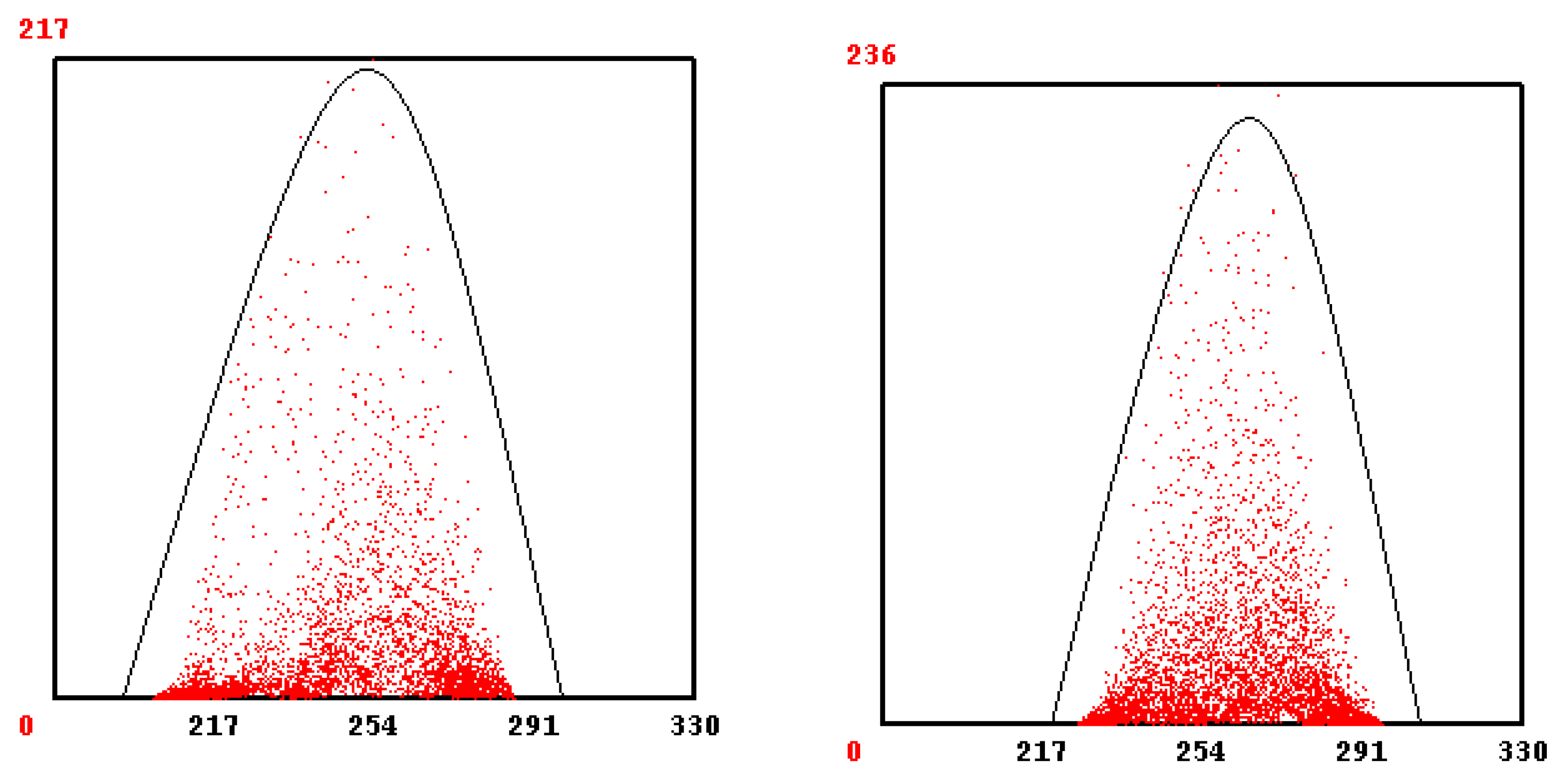
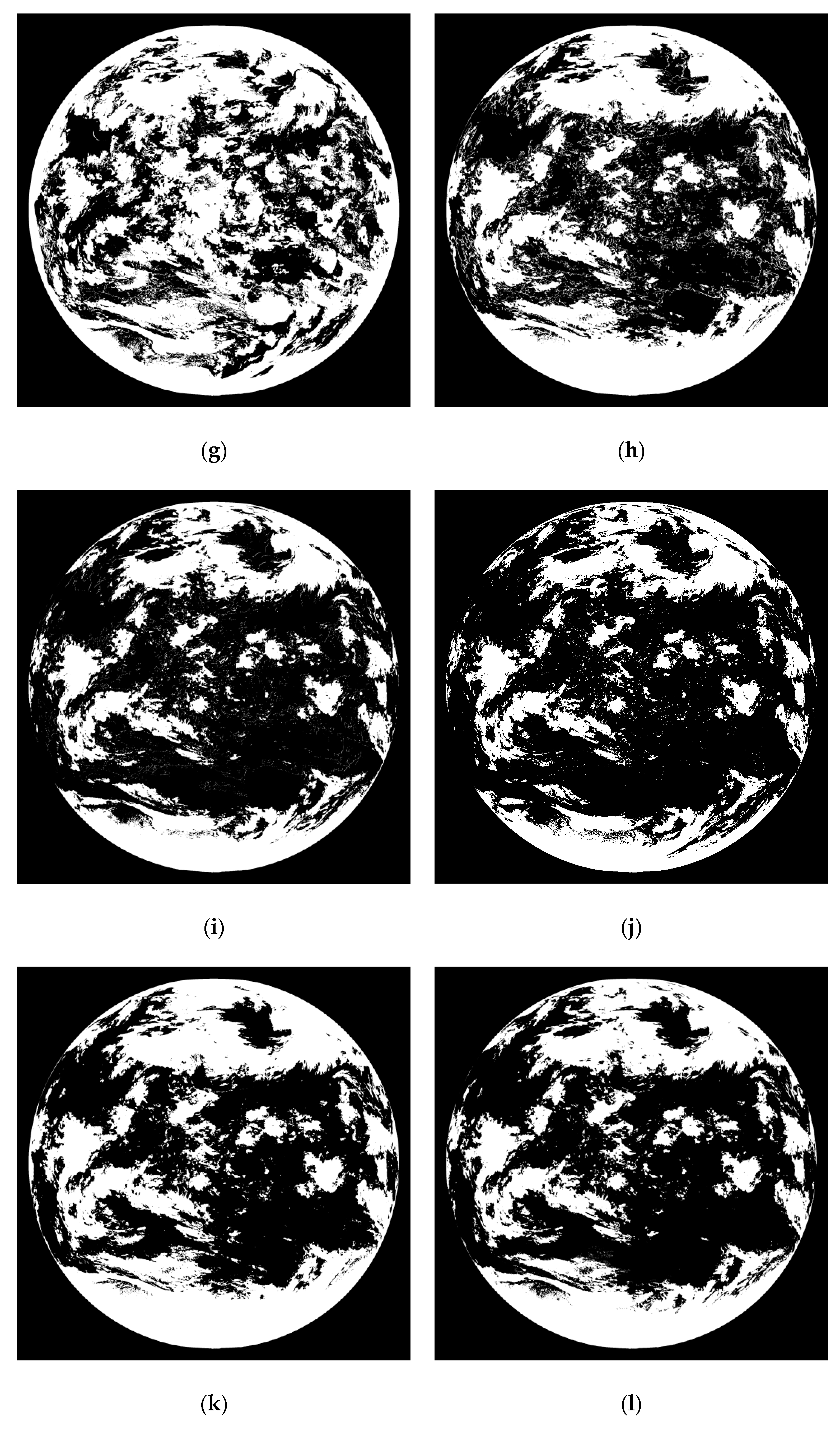
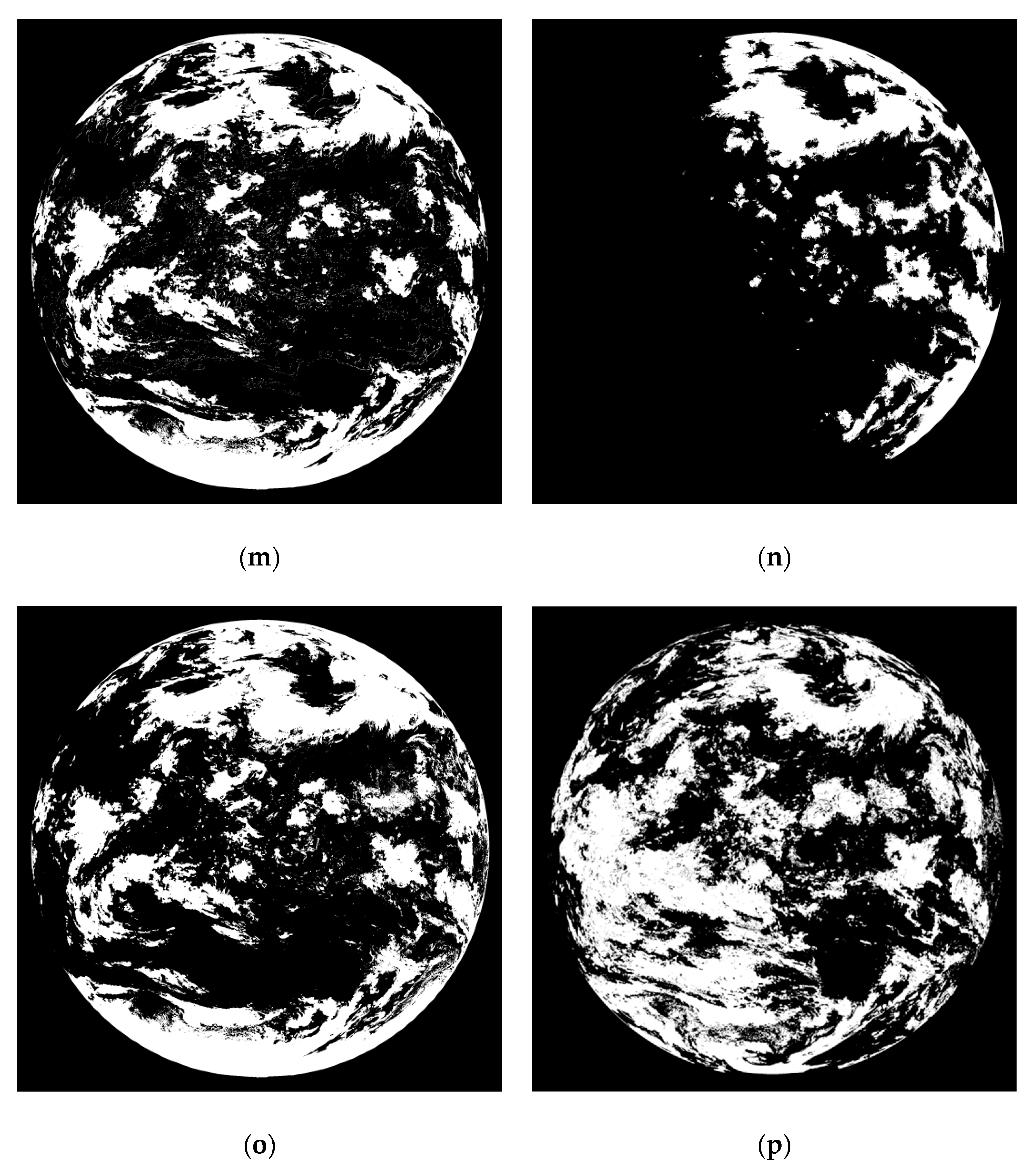
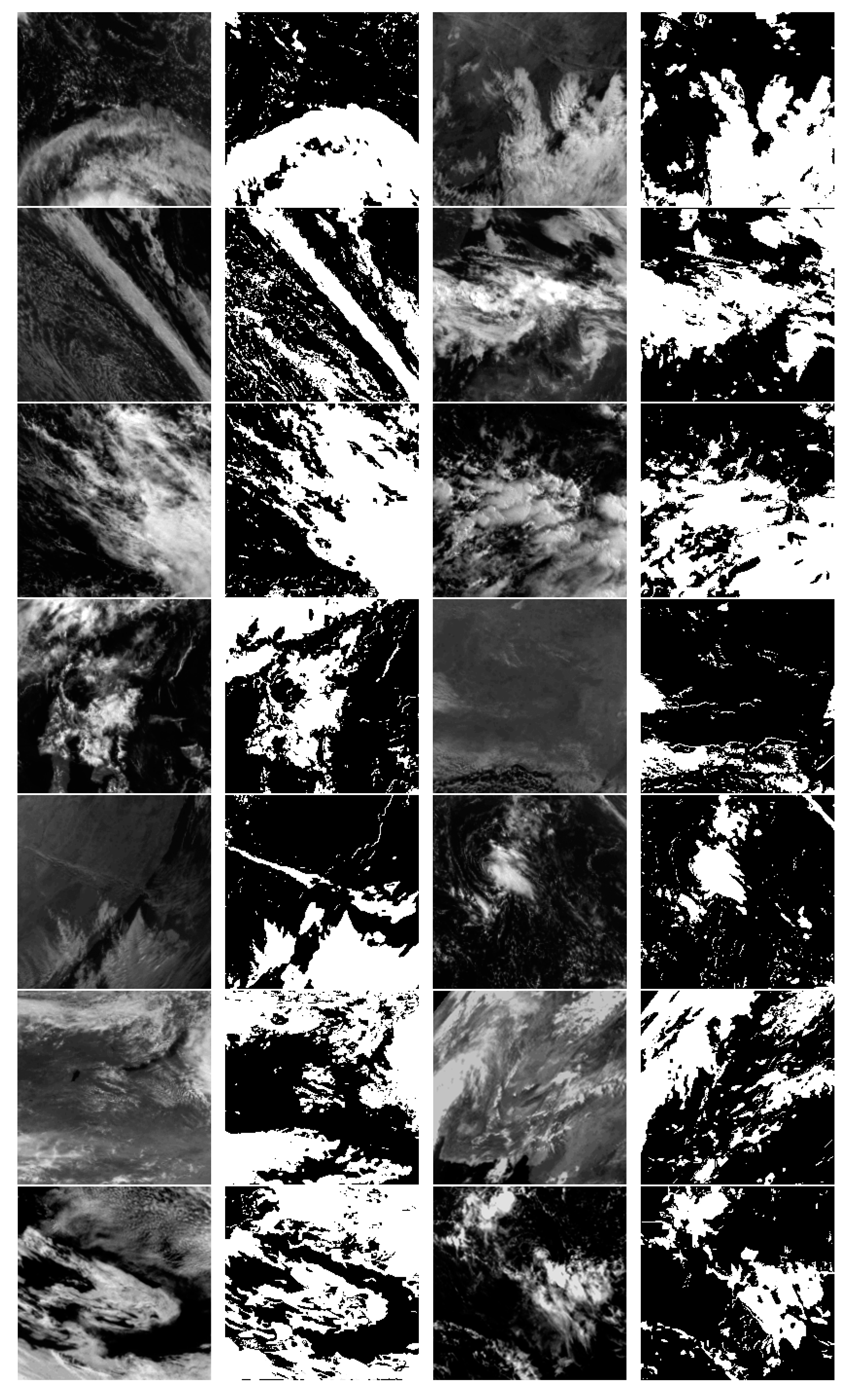
We use the IR1 and VIS images at 8:00 on 3 June 2015 for ensemble threshold analysis. The results of the cloud detection for each threshold method are as follows. It should be noted that the IR1 image and the VIS image in the following figure were enhanced for better display using linear transform.

Figure 6c–l are results of ten employed threshold-based methods using IR1 image, and limited to page length, the single result of each method using the VIS image is not shown, which is more or less the same as the corresponding IR1 result. From Figure 6, we can see that different threshold-based methods show different performance, and there are many misdetection regions for a specific method. For example, the block OTSU method can better preserve local cloud information. It can judge the land and water area as non-cloud correctly. However, the cloud detection performance at the bottom of the image is poor. For Wellner’s adaptive threshold method in Figure 6f, it can be seen that this method performs poorly at the marginal areas, but it performs well locally, and can identify non-cloud areas well. This situation is normal as expected, since the binarization capacity of a threshold is limited. By integrating the results of all the threshold-based methods, as shown in Figure 6n, and comparing with the original IR1 and VIS images and the NSMC result, we can find that in the central areas, the ensemble result shows very good performance in cloud detection and there are not so many misdetections. However, for the surrounding areas, especially for the bottom areas, the ensemble threshold method shows much poorer performance than the NSMC result. It is obvious that the ensemble threshold method treats many non-cloud areas as cloud areas while the NSMC result could distinguish non-cloud and cloud areas well in these regions. At the same time, there are partial misdetections at the central of the NSMC cloud detection results. But the cloud detection results at the upper and bottom areas of the NSMC show good performance. Therefore, we use the upper and bottom areas of the NSMC and the central part of the ensemble threshold result as the sample selection for the RF model.

3.4. Comparison of Various Cloud Detection Methods for Source Data at 16:30 on 17 March 2015

In this section, we improve the experiment based on the above results in Section 3.3. The upper and lower 1/4 portions of the NSMC result and the middle 1/2 part of the ensemble threshold result are taken as the samples to generate the training data set which is used for training in RF, and the test result of RF is compared with the NSMC result.

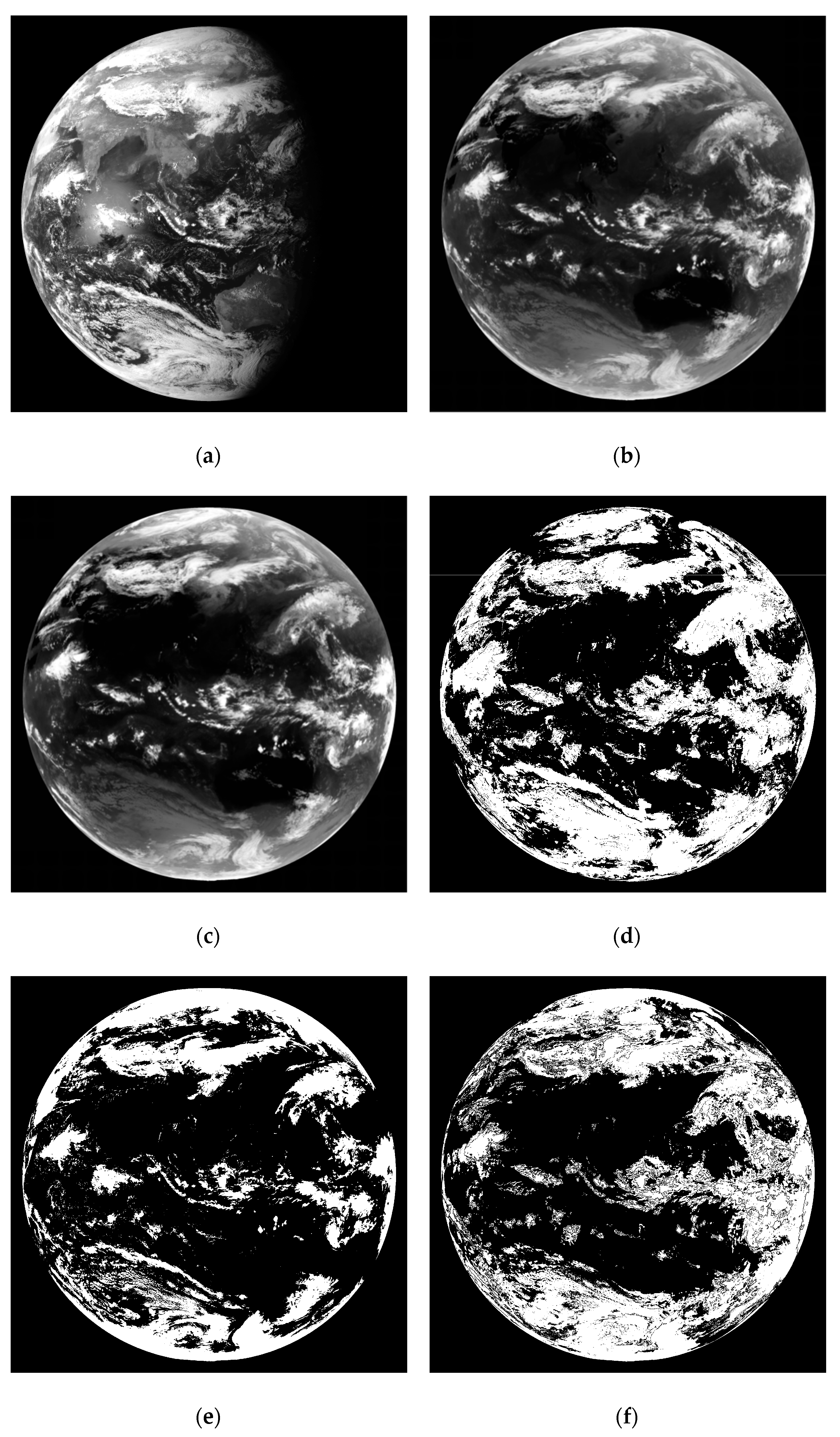
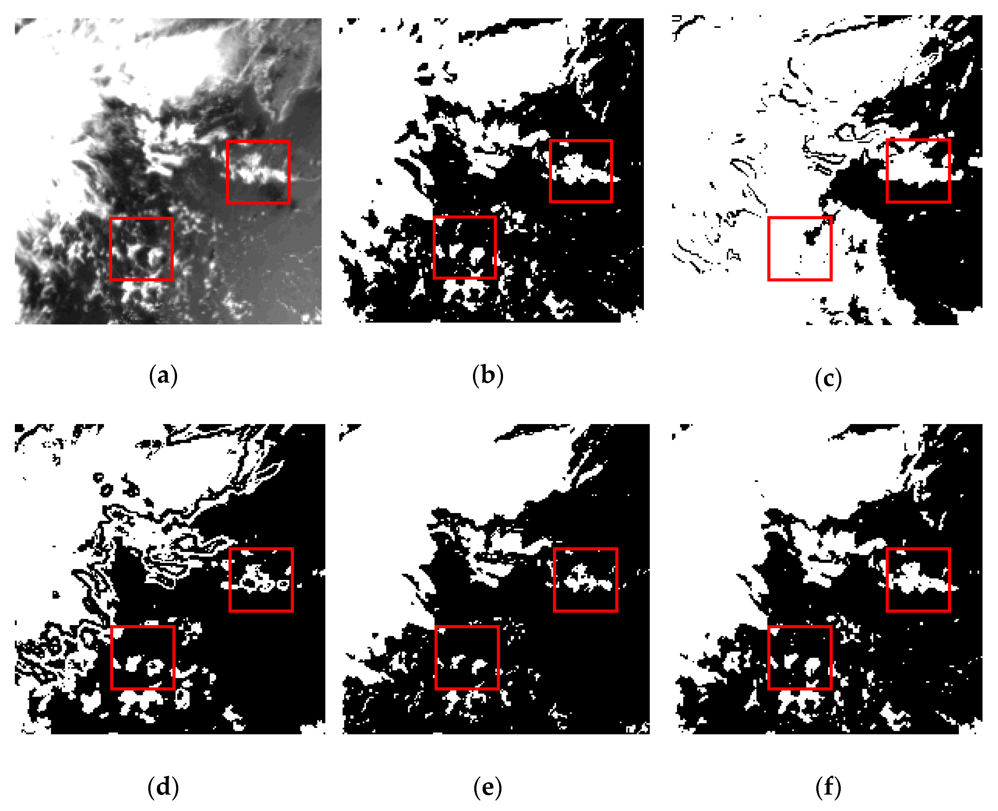
The test data used in this experiment is obtained at 16:30, on 17 March 2015, a different date to the training model. The original images and cloud detection results using different methods are shown in Figure 7. It should be noted that the IR1, IR2 and the visible images in the following figure are enhanced using linear transform for better display.

Compared with original VIS and IR1 images, the original NSMC result in Figure 7d shows many more detection regions which is slightly improved by NSMC-RF result in Figure 7f, however there are still many misdetection regions in the NSMC-RF result. The ensemble threshold result still has poor performance at the upper and lower parts, but with good performance at the middle areas. The ensemble threshold-RF result in Figure 7g is worse than the original ensemble threshold at the upper and lower parts. These results indicate that the incorrect samples of RF model will lead to worse performance, since the original NSMC result obviously has more detection regions and the original ensemble threshold result shows many wrong detections at the upper and lower parts. The proposed RF result in the Figure 7h makes up the deficiencies between NSMC and ensemble threshold-based RF models, which can be seen from the better performance on the accurate cloud regions and upper and lower parts.

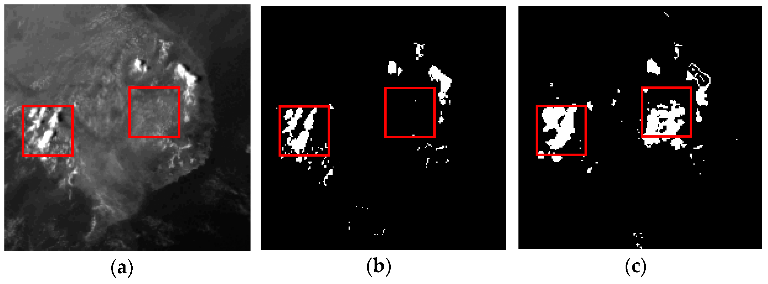
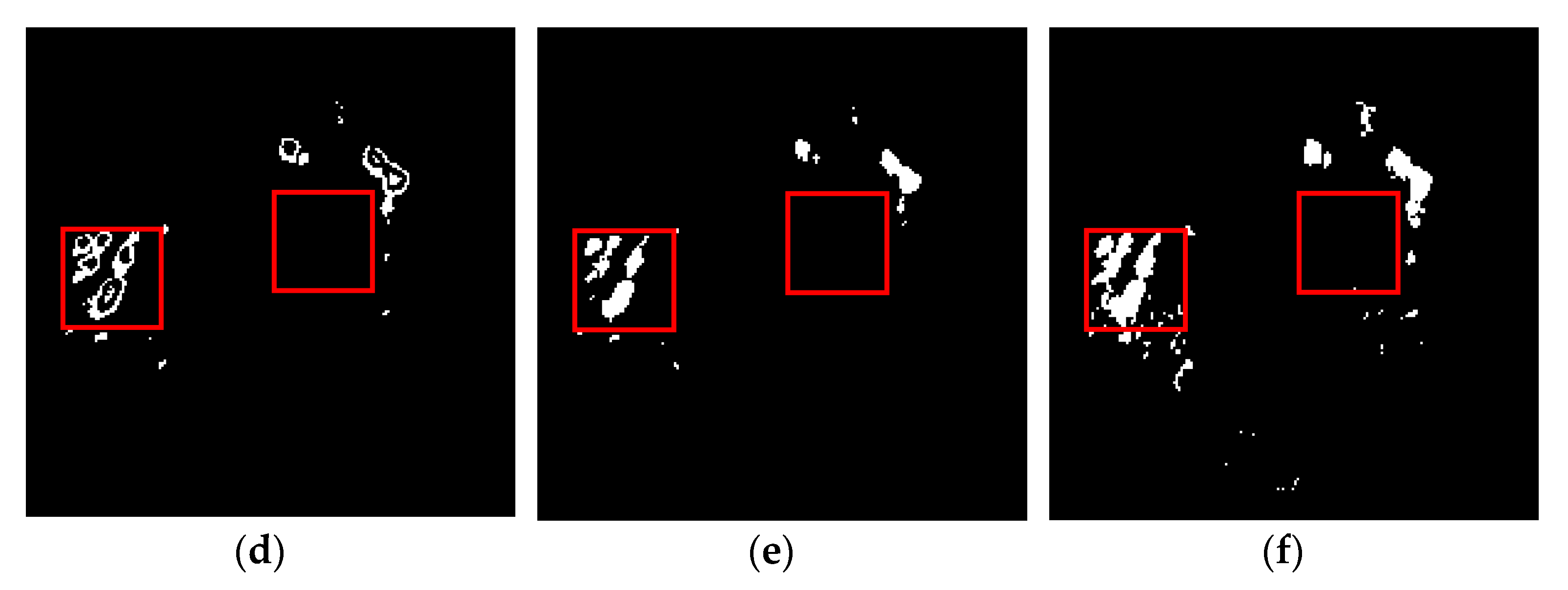
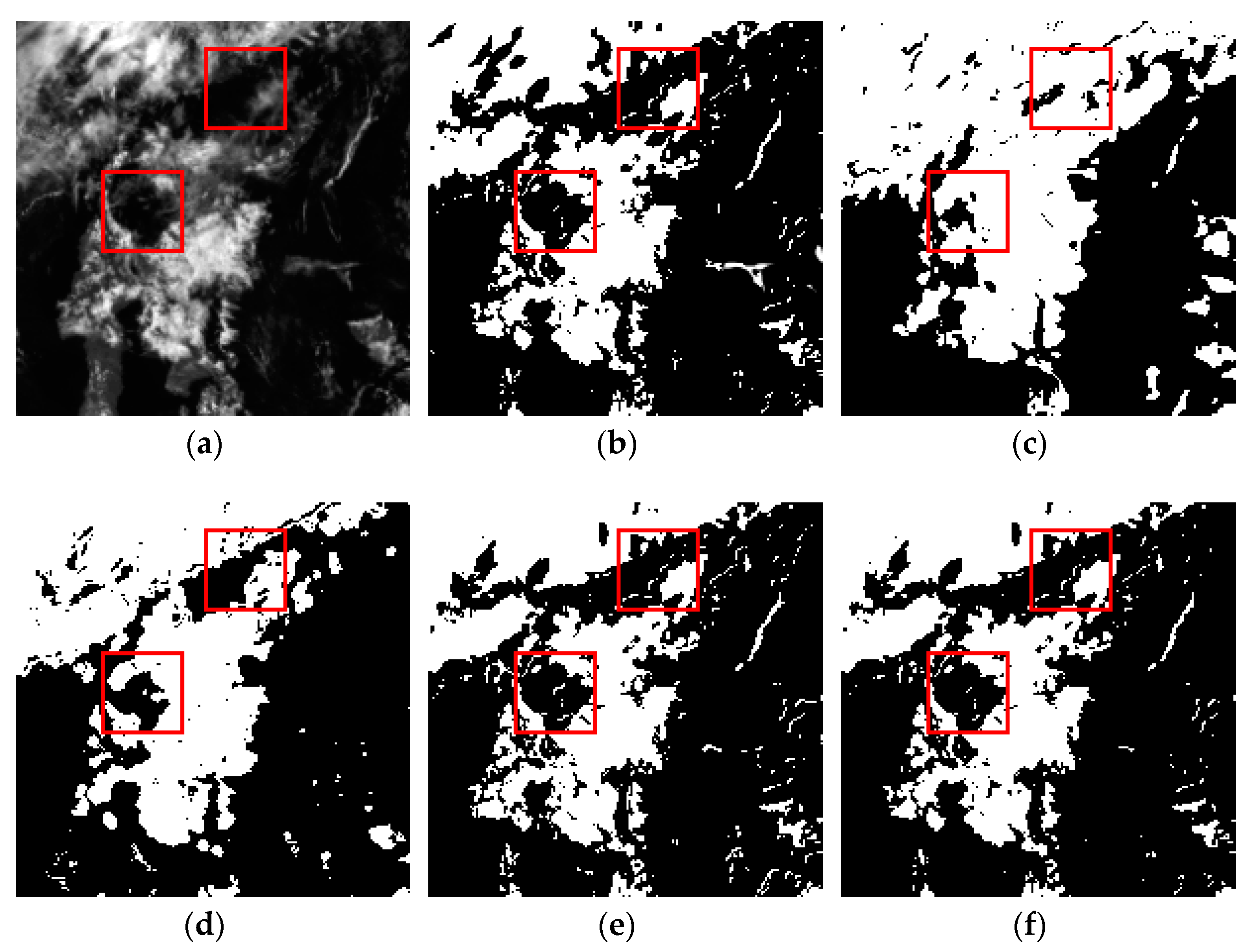
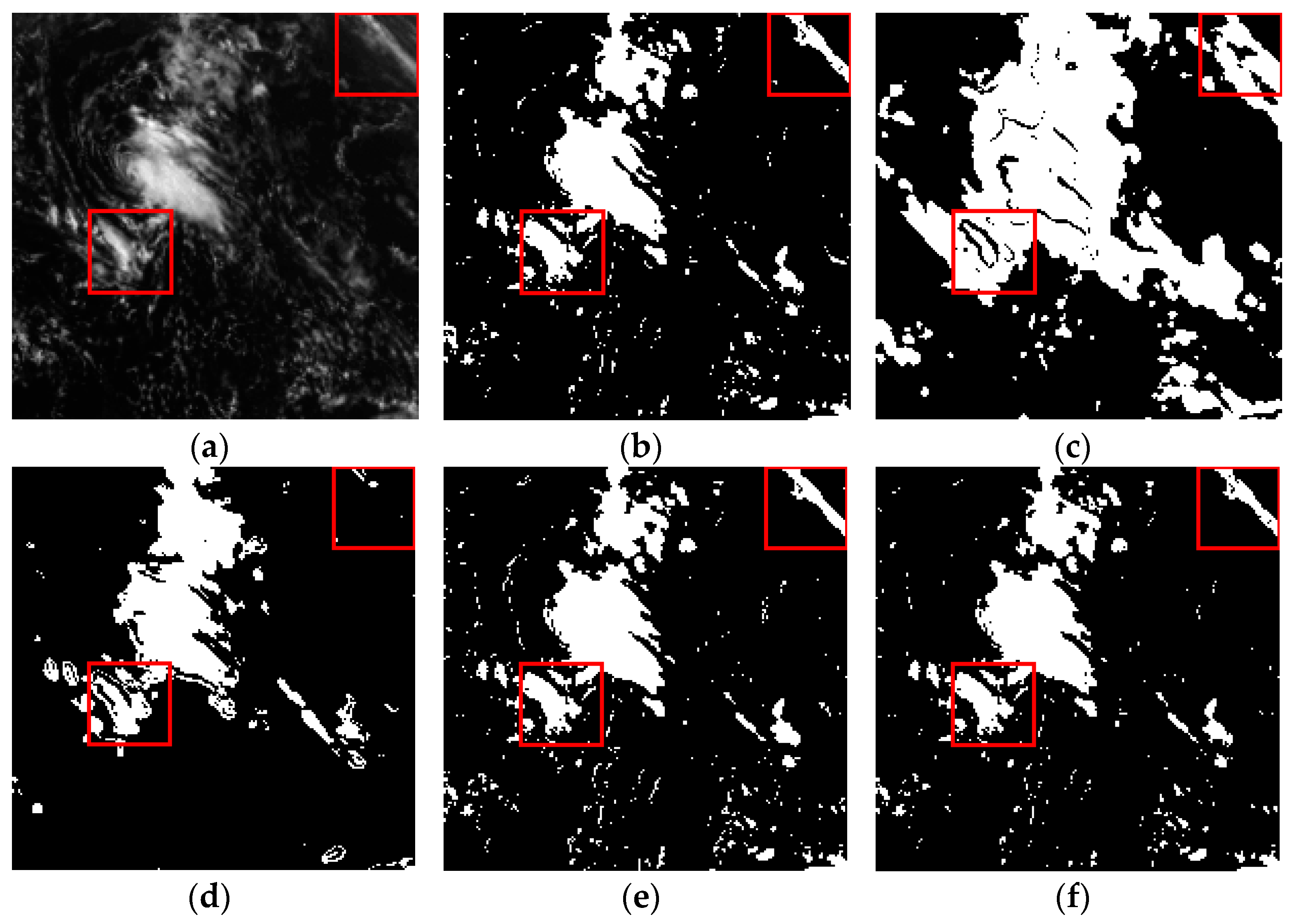
We manually label the thin and thick clouds in some areas as the ground truth to better illustrate the above experimental results, and the comparison results are shown in Figure 8, Figure 9 and Figure 10. The performance could be compared through the differences in the regions with red rectangles.

From the above figures, it can be seen clearly that the original NSMC results have many more detections in Figure 8c and (c and less detections in Figure 10c, while the NSMC-RF results show a little improvement in more detections but still have many incorrect detection regions. The ensemble threshold-RF results show better detection performance than the NSMC and NSMC-RF results in the above three sub-images but still have some differences with the ground truths. The proposed RF results show the best performance since the detection results are similar with the ground truth.

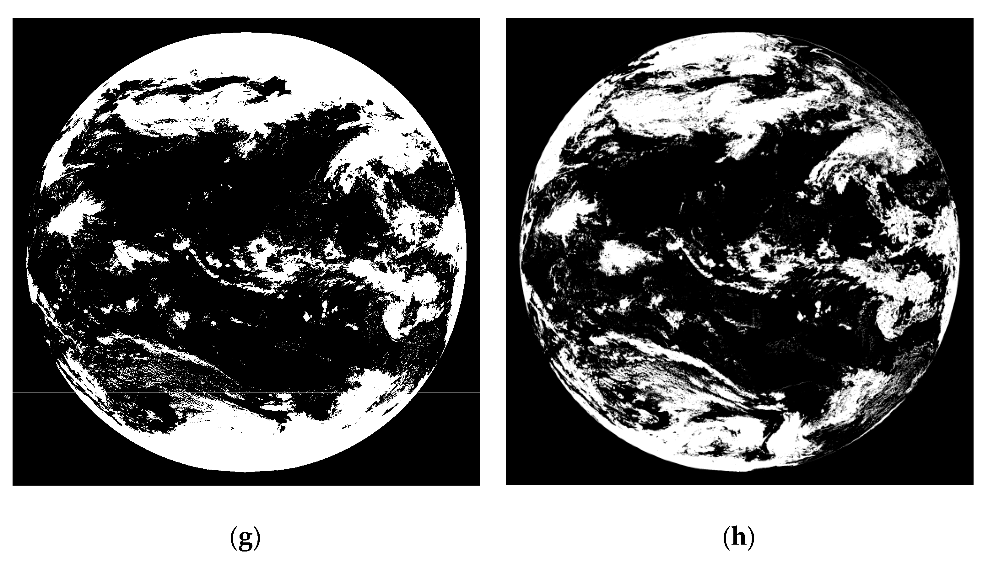
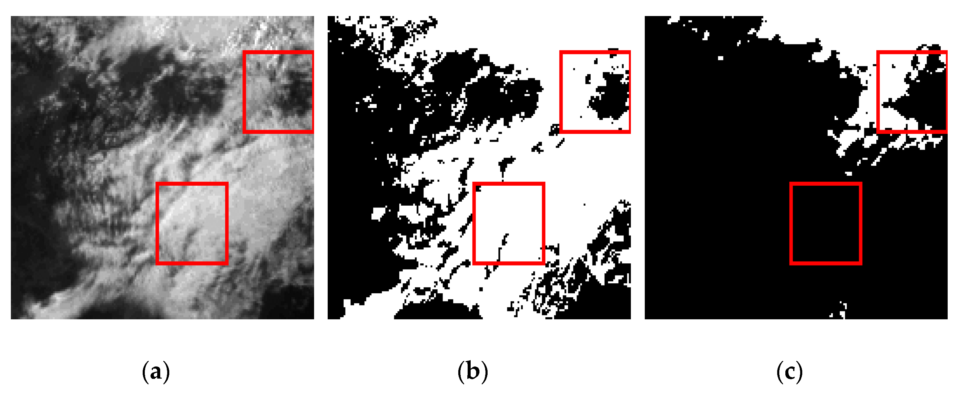
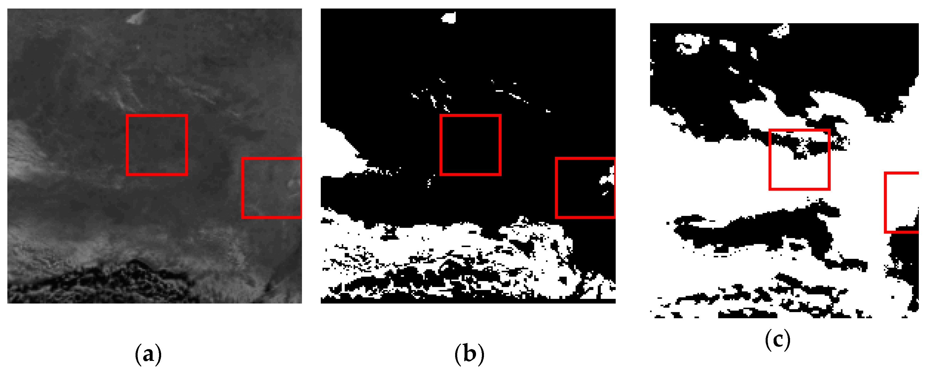
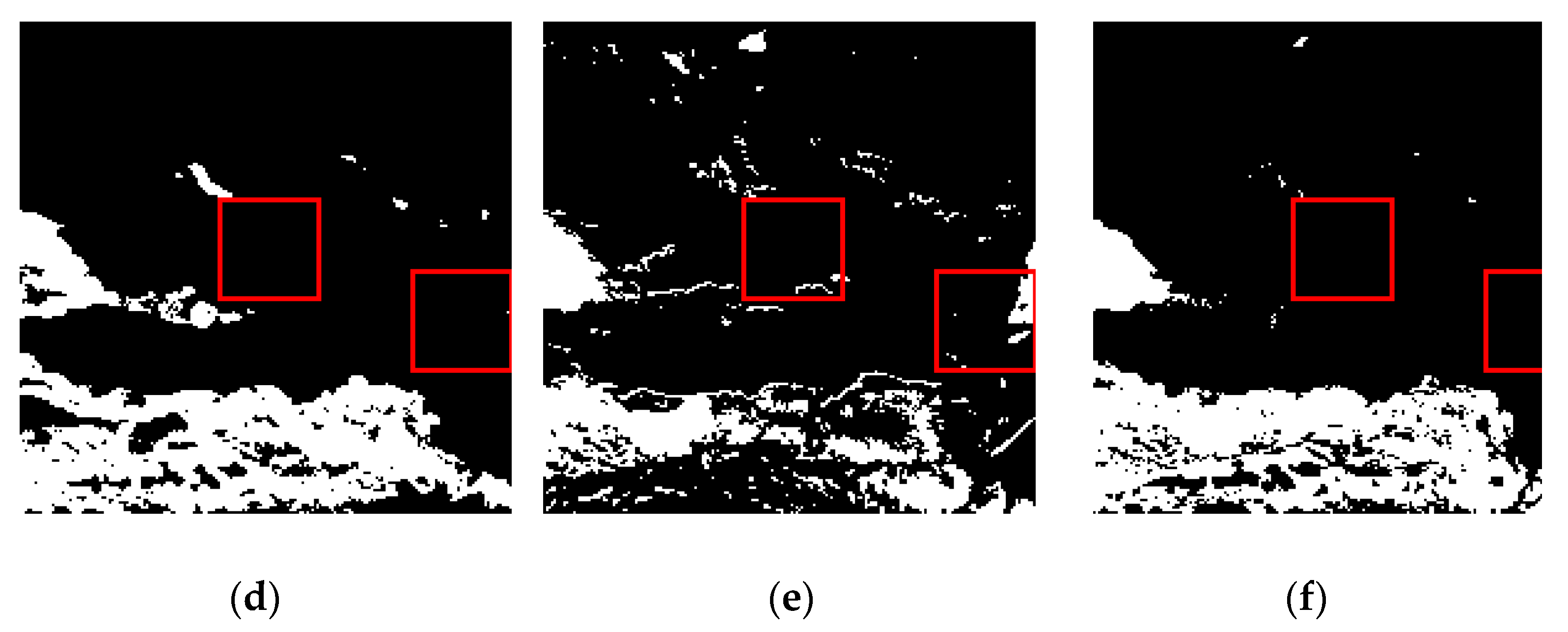
3.5. Comparison of Various Cloud Detection Methods for Source Data at 13:00 on 2 August 2015

Through the same method, we tested the proposed RF model on the image obtained at 13:00 on 2 August 2015, and the result is compared with the original NSMC, ensemble threshold, NSMC-RF and ensemble threshold-RF models. All the results are shown in Figure 11, and the original IR1, IR2 and visible images are enhanced for better display.

Comparing Figure 7 and Figure 11 we can see that the trends of differences between different methods are the same. The original NSMC result in Figure 11d has many more detection regions, and the NSMC-RF result in Figure 11f shows a slight improvement in reducing more detection regions. The ensemble threshold-RF result has worse performance in upper and lower parts but better performance in middle areas than that of the NSMC and NSMC-RF results. The proposed RF result takes into account the advantages of NSMC and ensemble threshold results and shows best performance in accurate cloud detection.

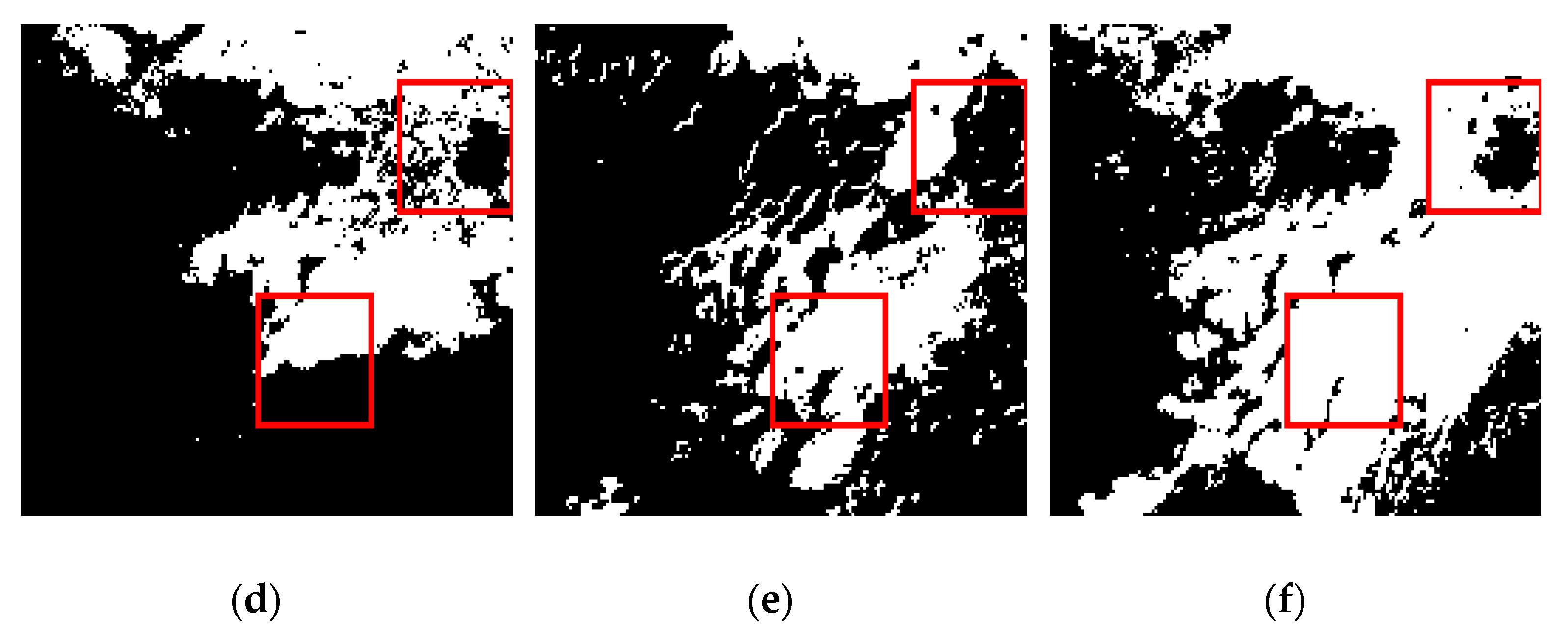
Figure 12, Figure 13 and Figure 14 show the cloud detection results in some sub-images covered by thin and thick clouds. The ground truth is manually labeled, and the red rectangles indicate the results with obvious differences.

Analogous to Figure 8, Figure 9 and Figure 10 in Section 3.4, we can find out that the NSMC results have much more obvious detection regions and NSMC-RF results show less more-detection areas. The ensemble threshold-RF results show better performance than NSMC and NSMC-RF results since the sub-images are obtained in the middle parts of original images. The proposed RF method could provide more accurate cloud detection results which are similar with the ground truths.

3.6. Objective Evaluation

To further compare the detection results, three evaluation indicators POD, FAR, CSI are used to objectively evaluate the performance of all employed methods including NSMC, NSMC-RF, Ensemble Threshold (ET), Ensemble Threshold-RF (ET-RF) and proposed RF. Sixteen sub images are randomly cropped from original images used in Section 3.4 and Section 3.5 and the corresponding clouds are manually labeled as the ground truth. Then all the detection results are compared with the ground truth and the objective evaluation is performed. 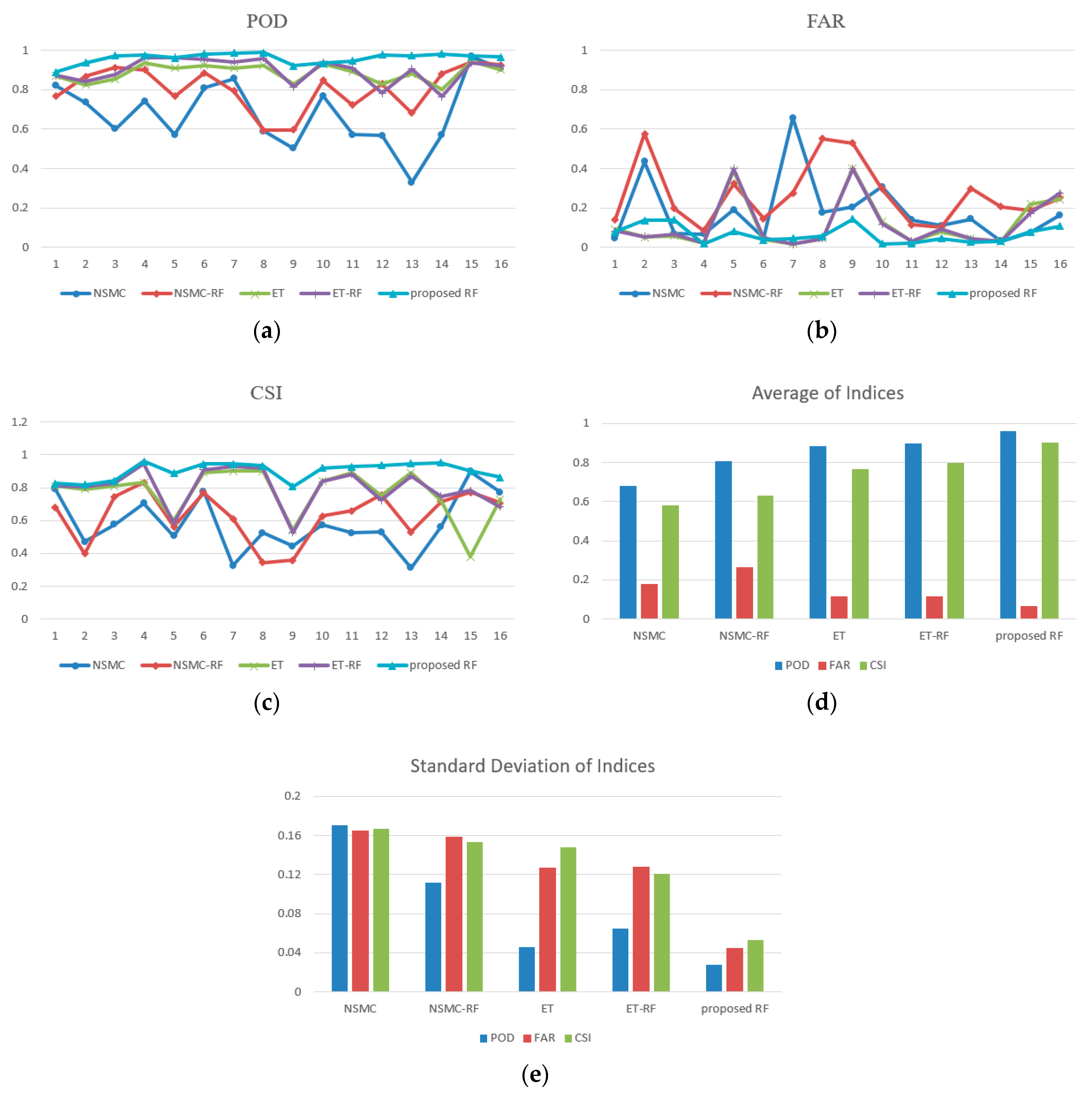The 16 sub images and corresponding ground truth are shown as Figure 15, and the 15th and 16th sub images are from the marginal parts of the whole images.

The evaluation results and the average and variance of each indicator are shown as Figure 16.

The POD values of the proposed method are always the highest, indicating that the real clouds are mostly detected as clouds. The curve of NSMC shocks between different images and almost shows the lowest POD values due to the misdetection of clouds. The ET and ET-RF methods also perform well, especially for the 15th and 16th sub images since the over detection of clouds. According to the definition of POD, the regions where the non-cloud is detected as cloud have no influence on POD value. Hence for ET and ET-RF methods, although for the 15th and 16th sub images they have over detection clouds, the POD is still high. However, in this situation, their FAR values are also higher than the other methods since FAR is an index which is sensitive of the regions where non-cloud is detected as cloud. In some sub images, the NSMC and NSMC-RF results show higher FAR values indicating that they have many incorrect detection regions. The CSI is a comprehensive index that takes into account the more detection and less detection regions. From the CSI index, we can see that the proposed RF method performs best in all cases and the other methods shock heavily between different cases. The ET and ET-RF methods are better than NSMC and NSMC-RF methods except for the 15th and 16th cases, since these two cases are from the marginal areas. The average indices show that the proposed RF method has highest POD and CSI, and lowest FAR; the ET-RF and ET methods have similar performances. The standard deviation of indicator aims to evaluate the stability when the methods are used in different cases, and the results indicate that the proposed RF method could provide more stable cloud detection results.

4. Discussion

An important task for meteorology satellite is to monitor the dynamic changes of clouds. Therefore, the accurate cloud detection is essential for meteorology satellite image processing since it is the first step after the image acquisition. The NSMC provides the official operational cloud detection products. In practical application, there still exists some regions with incorrect detection results. Considering that there are few cloud detection algorithms for FY meteorology satellite images except for the NSMC’s method, this paper proposes a new and ensemble cloud detection method via machine learning approach.

Compared with the NSMC’s algorithm, the proposed method has three features.

The first feature of the proposed method is the ensemble threshold method which could avoid the manual choosing of the threshold in many existing methods. Threshold-based binarization is a common technology in cloud detection algorithms, however the results of these methods mostly relay on the proper threshold. How to determine an optimal threshold is the main concern of these methods. Usually one threshold-based method could not generate satisfied result, but maybe more threshold-based methods could obtain a good result by majority voting, and this is the main principle of the proposed ensemble threshold method. In this paper, we use 10 widely used threshold methods to verify this possibility, and it really works well. Perhaps some methods are not the best, or some other methods are better, hence in the future, we will try many other threshold methods since the ensemble threshold methods are proven to be effective.

The second feature is very simple and the original random forest approach is directly used for cloud detection without complex feature selection. The features are just the original gray values and simple statistical variables of neighborhood pixels since we suppose that these values contain specific information of cloud and non-cloud areas. This simple approach is not the best way to use random forest, however, though it is so simple, it shows good performance. We provide a feasible way to use the machine learning approach to achieve high accuracy cloud detection. If more proper feature selection methods and advanced machine learning approaches are employed, the cloud detection performance would be better. The proper features could derive from image processing itself; maybe the features from atmospheric physical parameters could achieve more amazing results. As shown in [36,37], the water vapor plays a very important role in the relationship between aerosol and cloud for all cloud heights. The physical parameters such as aerosol optical depth, cloud Fraction, cloud optical depth, water vapor and cloud top pressure and other satellite-based parameters may have huge potential in accurately distinguishing cloud and non-cloud areas, or even recognizing cloud types and cloud in different heights. Therefore, combining the machine learning technologies and physical parameters is one of our future aims.

The third feature is that the training model on one image of a moment could be used for another image of another moment. For example, the data at 8:00 on 3 June 2015 is trained, and the model performs well on image at 16:30 on 17 March 2015 and 13:00 on 2 August 2015. This transfer capacity could be very useful in practical application. However, as for other satellite images, there are some problems for this transfer capacity since the imaging condition and atmospheric radiation are different every day, while for the FY meteorological satellite, we find that this transfer capacity cloud works well for different days. Meanwhile, it should be noted that this transfer capacity might not be universal. For example, the model trained in summer maybe works less well for images of winter. In this case, perhaps more models are needed to cover all the situations. Fortunately, these situations in meteorology satellites are relatively simple. Hence, how to maximize this transfer capacity is our future aim.

5. Conclusions

Accurate cloud detection is an important step for the application of meteorology satellite images. For FY serial satellites, the officially provided cloud detection products perform well in most cases. However, in some local regions, there still exists some misdetections. To further improve the cloud detection accuracy, an ensemble strategy-based method is proposed. An integration of the ten threshold-based methods are used for majority voting; the result is then combined with NSMC’s cloud detection product to generate the training samples for random forest algorithm; and finally, the trained model is used to detect clouds in other images. The proposed approach is very simple and there is more room for further improvement. For example, a more proper ensemble strategy of different threshold methods could be helpful for improving the performance on marginal regions, and more proper feature selection could achieve higher accuracy. Meanwhile, more tests should be done for other FY serial satellite images to improve the stability of this approach. These are all the main focus in the future.