Indoor Topological Localization Using a Visual Landmark Sequence
by
 , , ,
, , ,
Jiasong Zhu
1, 
Qing Li
1,2,3,*,
Rui Cao
1,3,4,
Ke Sun
1,
Tao Liu
5,
Jonathan M. Garibaldi
2,
Qingquan Li
1,
Bozhi Liu
3 and
Guoping Qiu
2,3 1
Shenzhen Key Laboratory of Spatial Smart Sensing and Services & Key Laboratory for Geo-Environmental Monitoring of Coastal Zone of the National Administration of Surveying, Mapping and Geoinformation, Shenzhen University, Shenzhen 518060, China
2
School of Computer Science, The University of Nottingham, Nottingham NG8 1BB, UK
3
College of Information Engineering & Guangdong Key Laboratory of Intelligent Information Processing, Shenzhen University, Shenzhen 518060, China
4
International Doctoral Innovation Centre & School of Computer Science, The University of Nottingham Ningbo China, Ningbo 315100, China
5
College of Resource and Environment, Henan University of Economics and Law, Zhengzhou 450046, China
*
Author to whom correspondence should be addressed.
Remote Sens. 2019, 11(1), 73; https://0-doi-org.brum.beds.ac.uk/10.3390/rs11010073
Submission received: 7 November 2018
/
Revised: 30 December 2018
/
Accepted: 31 December 2018
/
Published: 3 January 2019
(This article belongs to the Special Issue Mobile Mapping Technologies)
Abstract
:This paper presents a novel indoor topological localization method based on mobile phone videos. Conventional methods suffer from indoor dynamic environmental changes and scene ambiguity. The proposed Visual Landmark Sequence-based Indoor Localization (VLSIL) method is capable of addressing problems by taking steady indoor objects as landmarks. Unlike many feature or appearance matching-based localization methods, our method utilizes highly abstracted landmark sematic information to represent locations and thus is invariant to illumination changes, temporal variations, and occlusions. We match consistently detected landmarks against the topological map based on the occurrence order in the videos. The proposed approach contains two components: a convolutional neural network (CNN)-based landmark detector and a topological matching algorithm. The proposed detector is capable of reliably and accurately detecting landmarks. The other part is the matching algorithm built on the second order hidden Markov model and it can successfully handle the environmental ambiguity by fusing sematic and connectivity information of landmarks. To evaluate the method, we conduct extensive experiments on the real world dataset collected in two indoor environments, and the results show that our deep neural network-based indoor landmark detector accurately detects all landmarks and is expected to be utilized in similar environments without retraining and that VLSIL can effectively localize indoor landmarks.
1. Introduction
Topological localization is a fundamental component for pedestrians and robots localization, navigation, and mobile mapping [1,2]. It is compatible with human understanding as topological maps utilize highly abstracted knowledge of present locations. Represented by a graph, a topological map is a compact and memory-saving way to represent an environment, and thus is suitable for large-scale scene localization [3]. Each node of it indicates a region of the environment, which is associated with a visual feature vector to represent it. The vital problem of the technique is to design robust and distinctive features to represent nodes identically.
Many handcrafted features have been devised based on colors, gradients [3], lines [4], or distinctive points to represent the nodes. Previous work also entails learning the representation of the nodes using machine learning techniques [5]. However, most of them fail in dynamic indoor environments due to camera noise, illumination and perspective changes, or temporal variations. Another serious problem is that there are numbers of visually similar locations in the same environment, which further adds the difficulty of finding the proper visual location representation. Therefore, it still remains a challenging problem to find the robust visual representation for image-based indoor localization.
Exploiting semantic information from videos for localization is more feasible and human-friendly compared to conventional features or appearance matching-based methods. Finding matched features in large scenes is inefficient, and it often fails due to the amount of visually similar locations. In addition, matching multi-modality images is also a problem. Steady elements in the environment are robust representations of locations as they are salient and insensitive to occlusions, illuminations, and view variations. Their ground truth locations are also fixed and known.
In this paper, we propose a novel visual landmark sequence-based approach that exploits the steady objects for indoor topological localization. In the approach, sematic information of steady objects on the wall is used to represent locations, and their occurrence order in the video is used for localization through matching against the topological map. A topological map constructed with the prior of floor plan map of the environment is used to store connectivity information between landmarks. Each node on the map indicates a local region of the environment and is represented by landmark sematic information. To address the environmental ambiguity problem, we extract landmark sequence from a mobile phone video, and match them using the proposed matching algorithm based on their occurrence order. We make the following original contributions:
- We propose a novel visual landmark sequence-based indoor localization (VLSIL) framework to acquire indoor location through smartphone videos.
- We propose a novel topological node representation using sematic information of indoor objects.
- We present a robust landmark detector using a convolutional neural network (CNN) for landmark detection that does not need to retrain for new environments.
- We present a novel landmark localization system built on a second order hidden Markov model to combine landmark sematic and connectivity information for localization, which is shown to relieve the scene ambiguity problem where traditional methods have failed.
Part of the content is included in our conference paper [6]. Compared to the conference paper, we show the following expansions:
- We modified the HMM2-based localization algorithm to make it work in the case where part of the multiple-object landmark is detected.
- We have conducted more comprehensive experiments to demonstrate that our landmark detector outperforms detectors based on handcrafted features.
- We further tested the algorithm in a new experimental site to verify the generality of the detector and the localization method.
- We also conducted further analysis over the factors, including landmark sequence length and map complexity, that affect the performance of the algorithm.
The rest of the paper is organized as follows. In Section 2, we review related work on visual landmark representation and image-based localization. In Section 3, we illustrate the basic concept of visual landmark sequence-based indoor localization. Section 4 presents the detail of the CNN-based detector, which detects landmarks from smartphone videos. Section 5 elaborates the proposed matching algorithm based on a second order hidden Markov model. Section 6 presents extensive experimental results, and Section 7 concludes the paper.
2. Related Work
The proposed method is highly related to visual landmark representation and image-based localization methods. We briefly review related works in the two fields.
2.1. Visual Landmark Representation
Visual landmarks can be divided into two categories: artificial landmarks and natural landmarks. Artificial landmarks are purposefully designed to be salient in the environment. Ahn et al. [7] designed a circular coded landmark that is robust with perspective variations. Jang et al. [8] devised landmarks based on color information and recognized them using color distribution. Basiri et al. [9] developed a landmark-based navigation system using QR codes as landmarks, and the user’s location was determined and navigated by recognizing the quick response code registered in the landmark’s location. Briggs et al. [10] utilized self-similar landmarks based on barcodes and were able to perform localization in real time. Artificial landmarks can be precisely detected since they are manufactured based on prior rules. Such rules allow them to stay robust, facing challenges of the varying illuminations, view points, and scales in images, and help to devise the landmark detectors. Their position can also be coded in the landmark appearance. However, deploying artificial landmarks changes building decorations, which might not be feasible due to economic reasons or the owners’ favor. Natural landmarks avoid changing indoor surfaces by exploiting physical objects or scenes in the environment. Common objects such as doors, elevators, and fire extinguishers are good natural landmarks. They remain unchanged over a relatively long period and are common in indoor environments.
Many methods have been proposed to represent locations using natural landmarks [11,12,13]. Some of them are based on handcrafted features, which make use of color, gradients, or geometric information. Planar and quadrangular objects are viewed as landmarks and are detected based on geometric rules [11,12]. Tian et al. [13] identified indoor objects such as doors, elevators, and cabinets by judging whether detected lines and corners satisfy indoor object shape constraints. SIFT features were chosen to perform natural landmark recognition in [14,15]. Serrão et al. [16] proposed a natural landmark detection approach by leveraging SURF features and line segments. It performed well in detecting doors, stairs, and tags in the environment. Kawaji et al. [17] used omnidirectional panoramic images taken in different positions as landmarks, and PCA-SIFT was applied to perform image matching. Moreover, shape [4,18], light strength [19], or region connection relations [20] have also been exploited to represent landmarks for localizations. Kosmopoulos et al. [21] developed a landmark detection approach based on edges and corners. These methods have achieved good results on specified objects in certain scenes. However, they are likely to fail in other scenes due to the variations in doors and stairs.
In this paper, we propose a robust landmark representation using sematic information. A CNN-based landmark detector is proposed to determine landmark type. Unlike previous approaches using handcrafted features, our detector learns the distinctive features to distinguish target objects and background. Moreover, it can be used for off-the-shelf scenes without changing. The learned features are not derived from a single space but from a combination of color, gradients, and geometric space. With a proper training dataset, it stays robust to landmark variations caused by illumination and other deformations. CNN was selected due to its high performance in image classification [22] and indoor scene recognition [23] and outperforms approaches based on handcrafted features.
2.2. Image-Based Localization
As mobile computing and smartphones are becoming readily accessible, there have been attempts to use smartphone cameras for indoor localization [17,24,25,26,27,28,29,30,31,32,33,34,35,36]. These methods exploit computer vision techniques to estimate people’s location and mainly fall into two categories: image retrieval-based methods and 3D model-based methods. The former uses images captured by the smartphone camera to search for similar images in the image dataset whose positions and orientations are already known. The pose of the query image is determined with poses of similar images. This approach not only requires significant offline processing but can also easily get stuck in situations where different locations have a similar appearance. The latter approaches estimate location by building corresponding 2D–3D matches. However, they do not work in low texture environments, and they suffer from image blurring caused by camera motion. In addition, environment change significantly decreases the performance of the two types of methods, which frequently occurs in indoor environments.
Many positioning algorithms have introduced landmarks for indoor localization. Basically, landmarks are taken as supporting information to reduce the error drift of dead reckon approaches [37,38,39]. In this paper, we focus on performing indoor topological localization with only visual landmark information since landmarks play an important role in localizing and navigating pedestrians in an unfamiliar environment [40].
Many approaches perform landmark-based localization under a geometric scheme. Triangle intersection theory is applied to localize users using more than three landmarks [41]. Jang et al. [8] presented an approach with a single landmark. The user’s position was estimated based on an affine camera model between the three-dimensional space and the projected image space.
Another type of landmark-based localization utilizes landmark recognition techniques. It assumes that users are close to the detected landmarks. The landmark is identified based on their visual representations [11,12,19]. However, in indoor environments, it is usually not feasible to match landmarks based only on visual features, since locations can have a similar appearance. Additional information is needed to distinguish different landmarks. Tian et al. [13] exploited textual information around doors to address this problem. However, it is not always possible to have tags of text around doors. Contextual information between landmarks was exploited through a hidden Markov model (HMM) to recognize landmarks and achieve good results in [42,43,44]. However, an HMM model only takes a previous landmark to recognize a current landmark and fails in scenes of high ambiguity.
In this paper, we propose a matching algorithm based on a second order hidden Markov model (HMM2) to utilize landmark connecting information and sematic information for landmark recognition. An HMM2 is able to involve the walking direction in the process of landmark recognition. The walking direction is introduced to constrain the landmark connectivity. In this manner, more contextual information is taken into account for landmark localization, so indoor scene ambiguity is reduced.
3. Visual Landmark Sequence-Based Indoor Localization (VLSIL)
We propose a novel visual landmark sequence-based indoor localization (VLSIL) framework, and we first illustrate its basic idea. Suppose there is an indoor space that has seven locations as shown in Figure 1a. For each location, there is a landmark representing it as shown in Figure 1b and the color indicates the landmark type. Pedestrians can only walk from one location to the others linked by a path. Suppose pedestrians reach the location L(2) without knowing it and observe the red landmark. Their locations cannot be determined since there is more than one location denoted by the red landmark (e.g., LM(5) and LM(7)). Suppose pedestrians observe red, green, and blue landmarks in sequence in their path. They can be sure they start from LM(2), go through LM(4), and arrive at LM(6), because LM(2), LM(4), and LM(6) are the only valid path. The VLSIL achieves localization through taking photos (video) of a location to determine the current position by matching a sequence of previously discovered landmarks against the topological map of the space.
4. Landmark Detection
The landmark detection process consists of two phases: the offline phase and the online phase. During the offline phase, landmark types are pre-defined from common indoor objects and scenes, and a CNN is trained to recognize them. The online phase performs the landmark detection from the captured videos. It includes frame extraction, region proposal, and landmark type determination. Figure 2 illustrates the whole process. The offline phase is highlighted with a light blue background, and the rest of it is the online phase.
In the real scene, many of the extracted images only capture the background information, which is usually representative of walls. Applying a selective search to these images is not necessary and decreases the efficiency. Therefore, we first determine whether the extracted image belongs to a wall (the background). If so, the next image is proceeded. If not, a selective search is performed, and proposed patches are identified.
The rest of this section provides a detailed introduction of the offline and online phases of the process.
4.1. Offline Phase
4.1.1. Landmark Definition
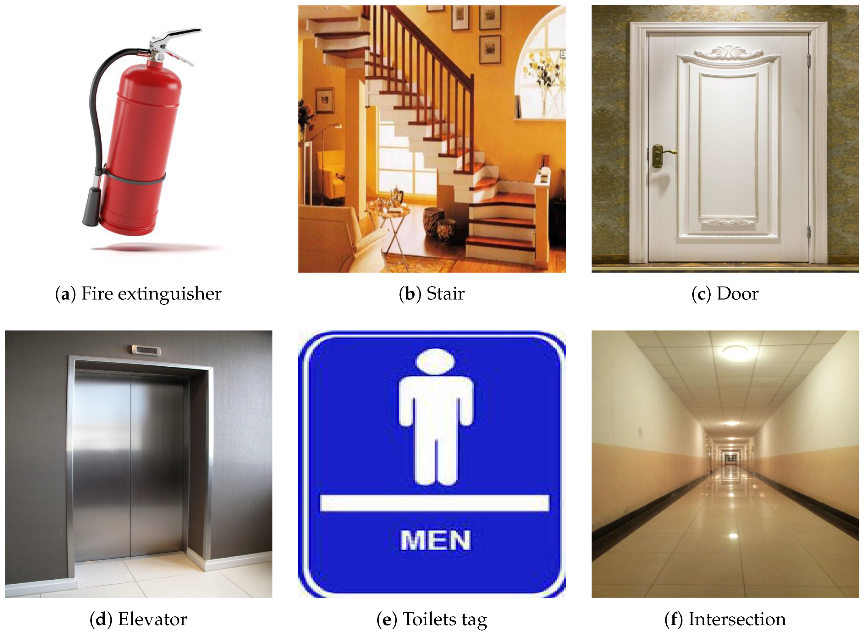
In this paper, landmarks are defined using common indoor objects such as doors, fire extinguishers, stairs, and indoor structure locations. Some examples of common objects are shown in Figure 3. Other indoor objects such as chairs and desks are not used because their positions are not fixed.
Three types of landmarks are defined: single-object landmarks, multiple-object landmarks, and scene landmarks. Single-object landmarks consist of one object such as a fire extinguisher or an elevator. Multiple-object landmarks are defined with more than one object. For instance, office doors are multiple-object landmarks, as they include a doorplate and a door. Combining multiple objects enlarges the landmark distinctiveness and reduces ambiguity of the map. We do not utilize the texts in the doorplate to further distinguish the office doors because motion blur makes text recognition very challenging. Scene landmarks are key locations of the indoor structure such as corners, intersections, or halls that have unique visual patterns.
4.1.2. Training CNN-Based Indoor Object Classifier
Our landmark detection relies on the object detection results of the extracted images. The high accuracy and real-time performance of the CNN on object detection inspired us to use it for our application [45]. In the application, we developed our CNN-based landmark detector by modifying AlexNet [46]. The modified AlexNet contains five convolutional layers and two fully connected layers. Each convolutional layer is tailed by a max pooling layer. Two fully connected layers are used to assemble information from the convolutional layers. AlexNet was selected for two reasons. The first is that its high performance in image classification has been demonstrated in ImageNet competition. Secondly, it is relatively easy to converge since it has relatively few layers compared to other more complex networks.
Several tricks were applied to train AlexNet for our indoor object detection. Firstly, the output layer was modified to recognize the target indoor objects. AlexNet was originally designed for ImageNet competition, which aims to recognize 1000 types of objects. However, not all indoor objects of our interest were included. We replaced the output layer with new one, in which the number of neurons equals the number of our interesting indoor objects. The softmax function was chosen as the activation function of output layer neurons. Secondly, we retrained AlexNet with a finetuning technique. Only the newly added layer was allowed to retrain, while the weights of the rest of the layers were fixed when fine-tuning. Finally, to eliminate the object variations caused by illuminations, rotations, and movement, we conducted data augmentation by pre-processing the original images. For each original image, we change its brightness by adding 10, 30, −10, and −30 to produce new images. We rotated the original image by 5, 10, −5, and −10. The movement of pedestrians led to the partial occlusion of targets of interest. We also generated new images by randomly cropping original images to sizes of . The brightness and rotating images were altered with the original images, and cropping was done in the training stage. In this way, we enlarged the training dataset, and the trained network was robust to those variations.
4.2. Online Phase
The online phase consists of frame extraction, region proposal, indoor object recognition, and landmark type determination. We elaborate the procedures in detail, except the indoor object recognition step, which simply feeds the image patches into the classifier.
4.2.1. Frame Extraction
During the online phase, smartphone videos are sampled at a given rate. The sampling rate is a vital parameter as it impairs landmark detection accuracy and efficiency. Low sampling rate results in low overlap or even no overlap between successive images, which leads to a loss of tracking of certain objects in the image sequence. A high sampling rate leads to large information redundancy, resulting in low landmark detection efficiency, as more images are to be processed. Overlap can be roughly estimated using Equations (1) and (2). They are applied in two scenarios: walking along a line and turning to another direction.
where V represents walking speed, and H is the average distance between camera and surrounding environment. is the field of view of camera in each mobile phone. represents sampling rate. is the angular velocity. Empirically, a sampling rate of 3–5 frames per second would work well.
4.2.2. Region Proposal
Cutting target objects out of extracted images is crucial for landmark detection. Feeding images that contain background and target objects directly into the classifier decreases object recognition accuracy. It is because training samples are covered with indoor objects in the majority of image space, while in extracted images target objects may occupy only a small part of it. Therefore, we have to crop the patches with target objects taking up most of the space. Here we choose the selective search algorithm to generate patches of interest from images [47]. Selective search employs a bottom-up strategy to generate patches. The process contains two steps. At first, an over-segmentation algorithm is applied to generate massive initial regions in a variety of color spaces with a range of different parameters. A hierarchical grouping approach is then performed based on diverse similarity measurements including color, texture, shape, and fill, with various starting points. Hundreds or thousands of patches are produced from the algorithm. However, we do not need to process all of them to identify the target objects since there may be too many eligible patches. The first 300 patches are normally used for accuracy and efficiency purposes.
4.2.3. Landmark Type Determination
Landmark type is determined based on the indoor object recognition results. For single-object landmarks and scene landmarks, their types are given with their corresponding indoor objects. Regarding multiple-object landmarks, their types are determined by the combination of detected objects. For instance, the combination of doorplate and door represents an office door landmark.
A sequence of images is used to perform landmark type determination instead of a single image. The main reason is that components of multiple-object landmarks might not appear in the same image. The recognition result of a sequence images can address the problem as the components are sequentially detected. Moreover, it is helpful to eliminate the wrong recognition results. In this paper, indoor objects that are not seen in three successive images are interpreted as false detections. Exploiting image sequences for localization also helps determine the landmark occurrence order when more than one landmarks are observed in a single image. The first landmark detected prior to the current landmark is viewed as the previous landmark of the current detected landmark in the sequence. Sequence image length is set automatically based on the recognition results. A sequence starts from an object, is robustly recognized, and ends at the images (the walls).
5. Visual Landmark Sequence Localization Using the Second Order Hidden Markov Model
Knowing a sequence of landmark types from a video, we match them with the predefined topological map. In this section, we illustrate the defined topological map and the matching algorithm based on the second order hidden Markov model (HMM2) for our applications. We also extend the Viterbi algorithm for our application.
5.1. Topological Map
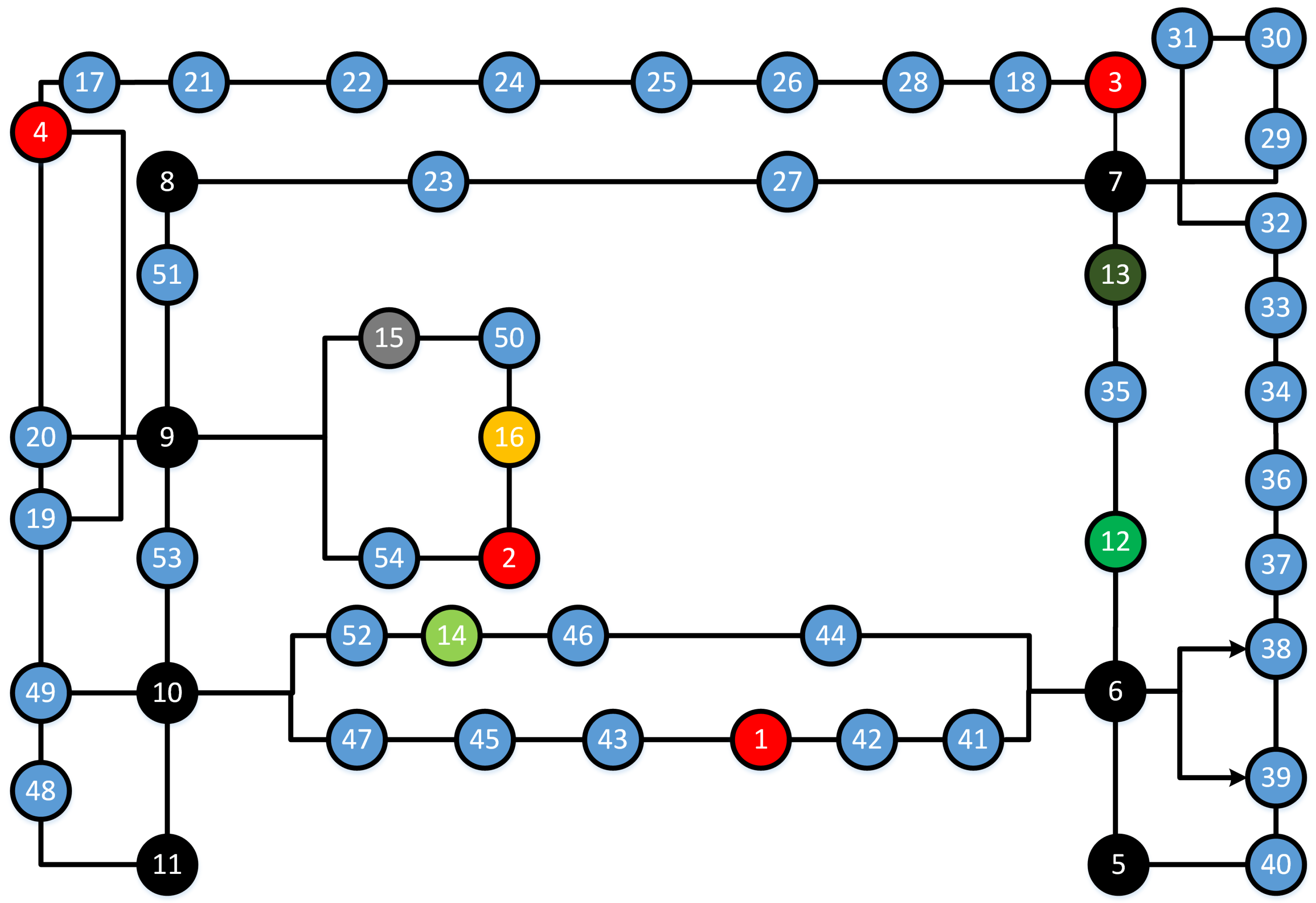
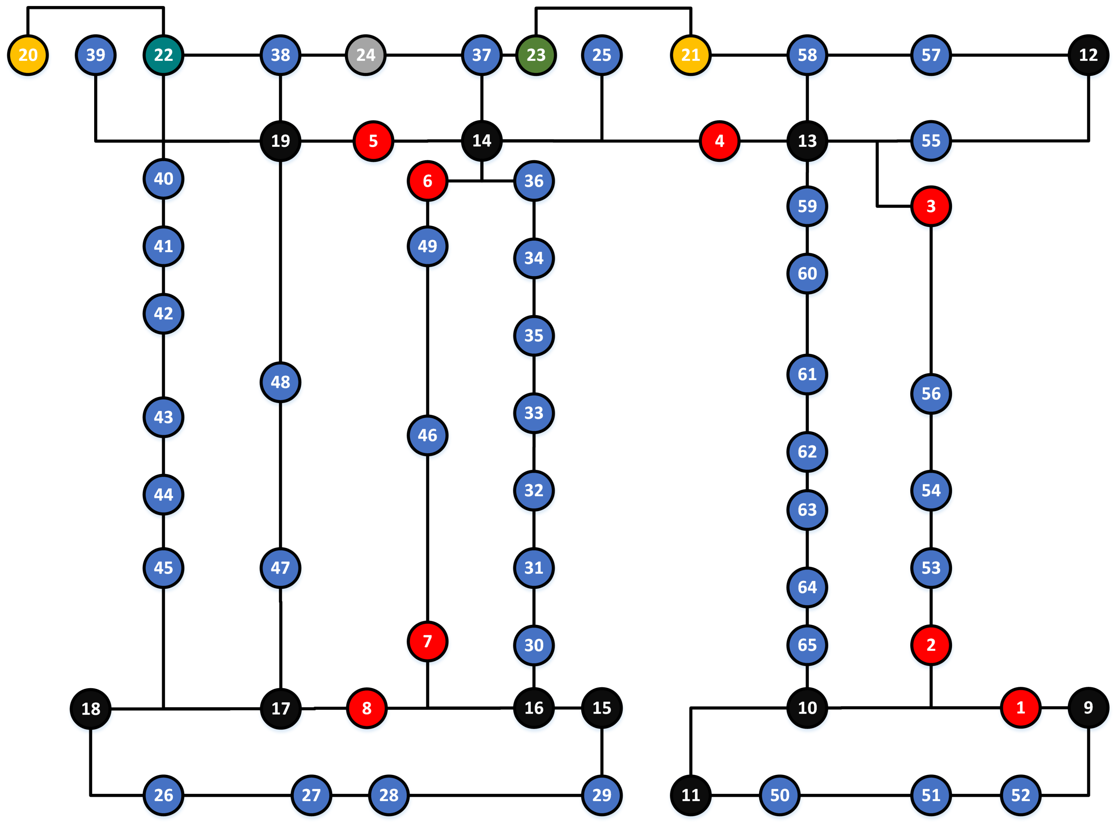
The topological map provides information of the distribution of landmarks of the indoor environment and indicates the connectivities between landmarks. In our paper, the topological map is a directed graph and is created from the floor plan map of the indoor environment. It consists of two types of elements: nodes and edges. Nodes indicate regions of the environment. Their color represents the landmark type. We use red nodes for fire extinguishers, black for intersections, blue for offices, silver for elevators, yellow for stairs, light green for the disabled toilets, green for men’s toilets, and dark green for women’s toilets. Edges denote the connecting information between landmarks. An edge starting from node i to node j indicates the sequential direction in which landmark j is detected after landmark i. The arrowed line indicates a one-way connection. In certain situation, two landmarks might be spatially close to each other. They are viewed as two regions and are represented with the corresponding landmarks.
5.2. The Second Order Hidden Markov Model for Indoor Localization
The HMM2 takes context information to perform tasks. It contains five elements: the observations set, the states set, the initial probability, the emission matrix, and the transition matrix. For our application, the observations set includes all landmark types and the states set indicates the landmark locations. Initial probability represents the starting position of a route. In the rest of the section, we detail the emission matrix and transition matrix of the HMM2 in our scenario. We also introduce a new parameter to handle unidentified multiple-object landmarks.
5.2.1. The Emission Matrix of HMM2
The emission matrix represents the state probabilistic distribution over the observation set [48]. Its row count equals the number of states and its column count is the number of observations classes. For our problem, the entry values of the emission matrix indicate the probability of an observed landmark type that belongs to a certain state. We assign the emission matrix value based on the landmark types of a landmark location. The emission matrix is defined as follows: , if landmark type j corresponds to state i; , otherwise.
5.2.2. The Transition Matrix of the HMM2
Unlike the transition matrix of the hidden Markov model which is a two-dimensional matrix, the transition matrix of the HMM2 is three-dimensional [48]. Its value indicates the probability that the next state is k, given the condition that the previous state is i and the current state is j. For the landmark-based indoor localization problem, it represents the probability of going through certain landmark positions given the previous two landmark positions. The matrix is defined as if there is a path from i through j to k; , otherwise.
5.2.3. The Probabilistic Matrix of Landmark Type
Ideally, multiple-object landmarks are correctly recognized. However, in some cases, only a component of the landmark is detected. To deal with the problem, a probabilistic matrix, , the probability of landmark type i given detected object j, is defined. This parameter does not affect single-object landmarks or scene landmarks. For them, when the object or scene is detected, its landmark type is determined. It aims to solve the confusion of multiple-object landmark when part of a landmark is observed. This works for situations where an object is detected but its landmark type still remains undetermined. The matrix value if landmark i is a single-object landmark and j is the object to form it; , otherwise. For multiple-object landmarks, if the detected object cannot be used to recognize landmarks, we split the probability evenly. For example, if a door is detected, its matrix value equals 0.25 since it could belong to either an office or a toilet.
5.3. The Extended Viterbi Algorithm for Indoor Localization
Given the modified HMM2 for landmark localization, we extend the Viterbi algorithm to find the landmark sequence corresponding to the sequence of landmark types based on Bayesian theory. The details are below. Assume that the HMM2 has M states for landmarks, and the initial state parameter is , which represents the probability when the process starts from landmark i. The transition matrix value is the transiting probability that the process move from landmark i to landmark j. There are n detected landmarks in the observation sequence, represented by . The corresponding locations are represented by We aim to find the landmark location sequence X of the maximum probability, given the landmark type sequence Y. Therefore, our objective function is to maximize . From the Bayesian theory,
where denotes the probability distribution of the landmark type sequence Y, given state sequence X. In the hidden Markov model (HMM), it is represented by the emission matrix. is the prior probability distribution of state sequence X. is the probability distribution of the observation sequence. It is a constant value. Hence, the solution to maximizing and maximizing are the same.
Since the logarithm function is monotonically increasing, and share the same solution for the maximization problem. Note that the HMM requires that the next state only depends on the current state. can be simplified to Equation (6).
The Viterbi algorithm is used to find the solution to the maximization of . It recursively computes the path. Two parameters are updated in the process. At any step t, is used to record the maximum probability of the landmark sequence ending at landmark k, given t observations. records the previous landmarks before landmark k in the most likely state sequence. The process is as follows.
The Viterbi algorithm has shown good performance in terms of solving the HMM problem. It has to be modified to solve the HMM2 problem because the HMM2 takes both the previous state and the current state into consideration when predicting the next step. Thus, Equation (6) has to be extended as follows.
Another issue is that, during landmark detection, the landmark type might not be clearly recognized. The modified equation is Equation (11). A parameter is added to represent such unclear observations as introduced in Section 5.2.3. The Viterbi algorithm for the HMM2 was initialized by Equations (12) and (13) followed by iteration Equations (14) and (15) and is summarized in Algorithm 1.
where is the object type of detected landmark t.
| Algorithm 1: Extended Viterbi finds the location sequence of maximum probability. |
| Input: A sequence of observations Y, transition matrix , emission matrix E, probabilistic matrix P, initial location Output: A sequence of states X
|
6. Evaluation
6.1. Setup
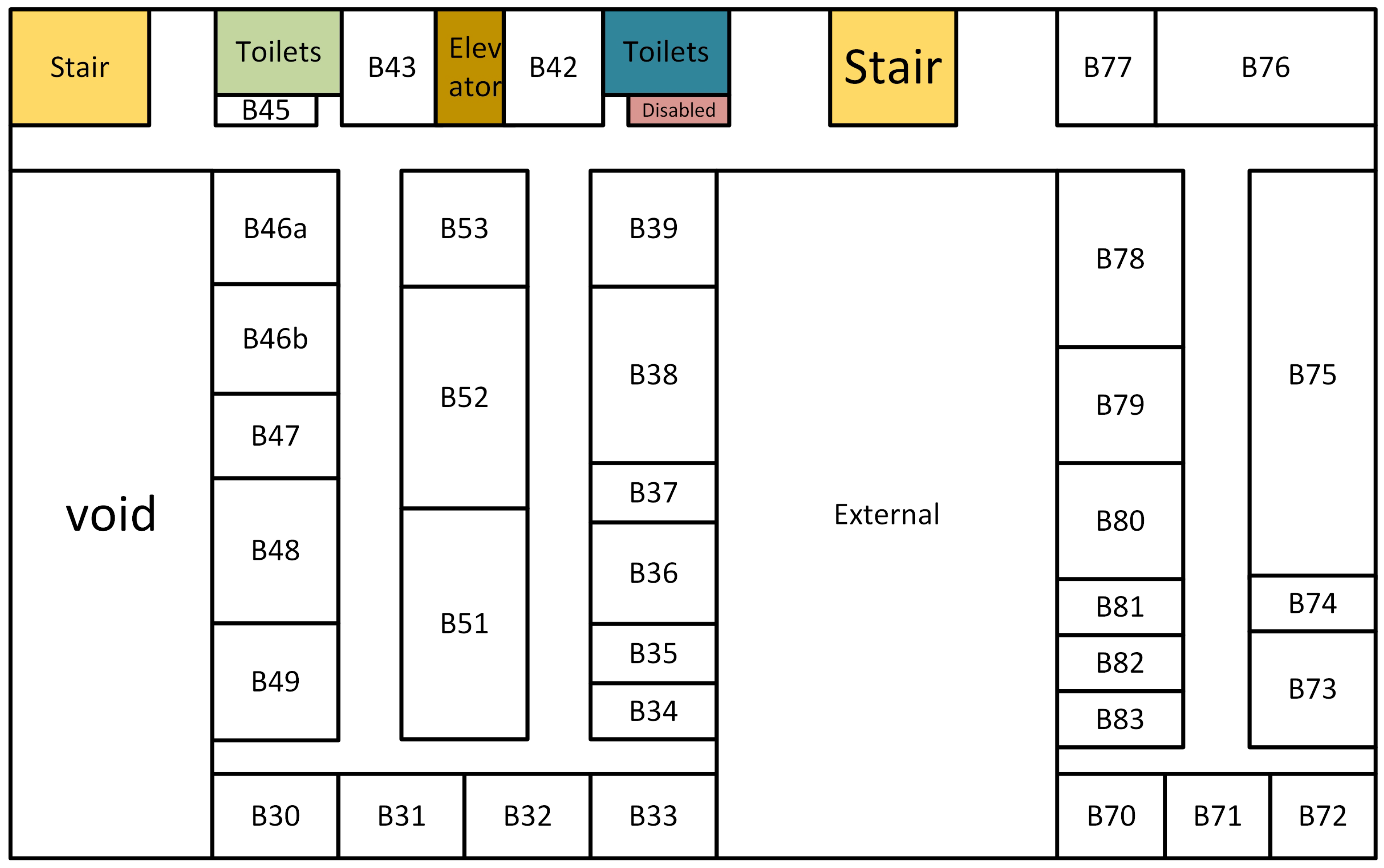
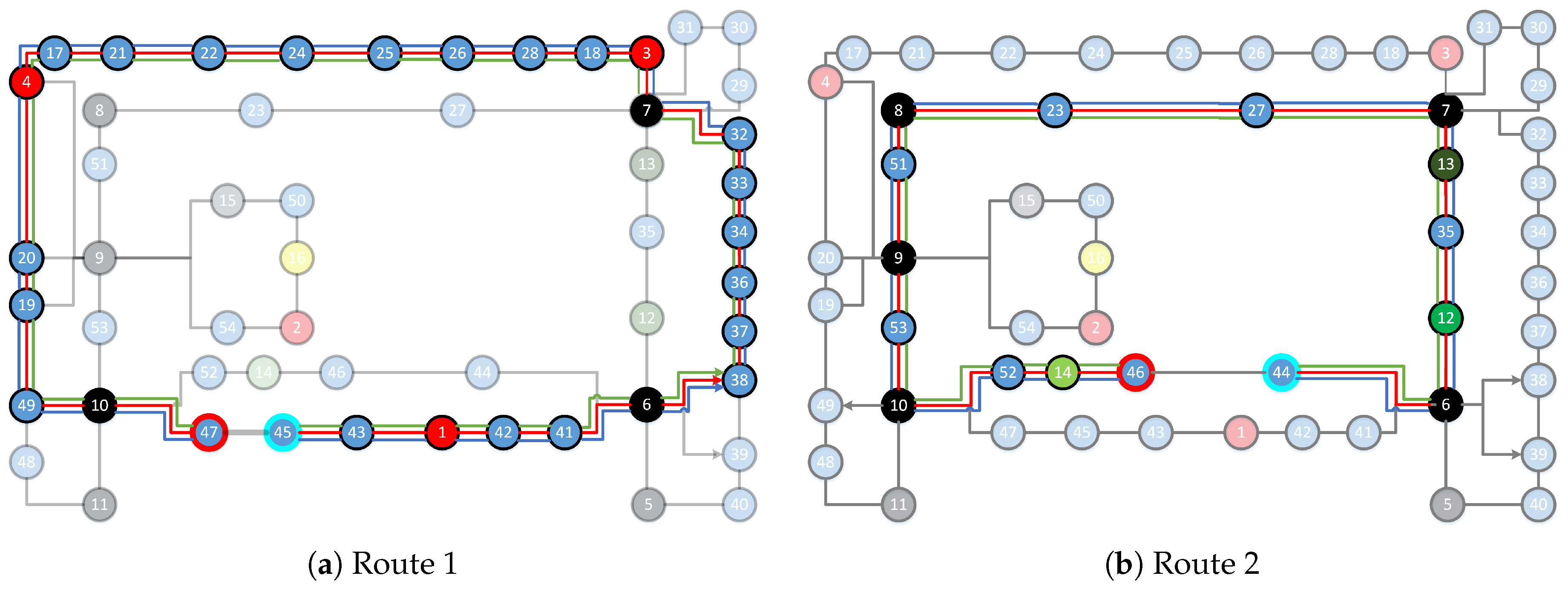
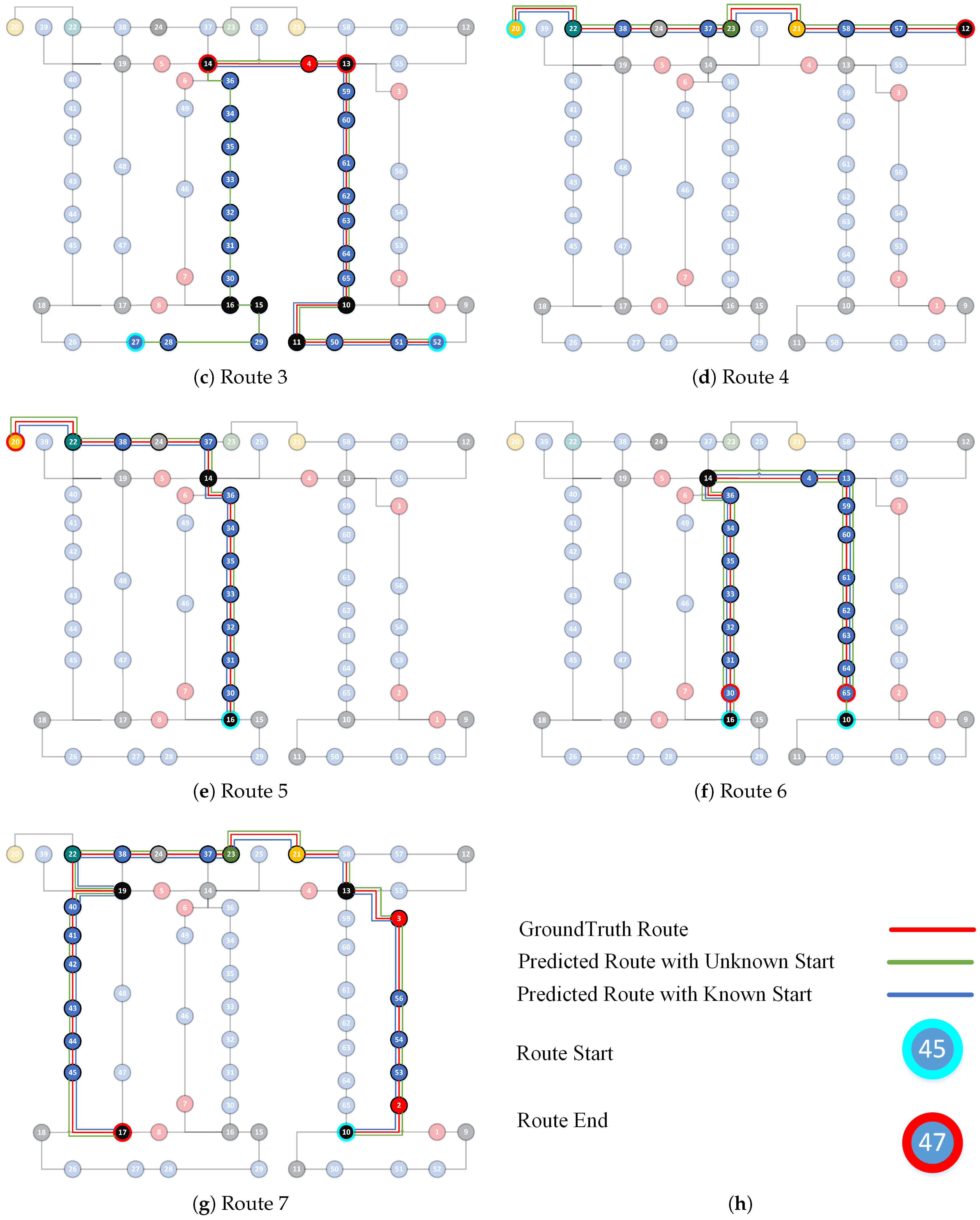
To evaluate the proposed method, we conducted our experiments on the B floor of the Business South building (BSB) and the B floor of the School of Computer Science building (CSB) at the University of Nottingham, UK. The two sites are typical office environments containing many corridors and office rooms. Floor plan maps of the two sites are shown in Figure 4 and Figure 5, respectively, and their corresponding topological maps are shown in Figure 6 and Figure 7. We selected eight types of landmarks from the two places: office rooms, stairs, elevators, fire extinguishers, men’s toilets, women’s toilets, disabled toilets, and the intersection (corner). Among them, fire extinguishers, stairs, and elevators are single-object landmarks. Office rooms and toilets are multiple-object landmarks. An intersection is a scene landmark. The BSB is a relatively simple environment, while the CSB is more complex. In the BSB, there are 54 landmarks in total, and there are 65 landmarks in the CSB.
Two female and three male participants were asked to collect videos at both sites using smartphones. Three models of mobile phones were used: an Huawei Honor, a Samsung Note 3, and an iPhone 6s Plus. Each participant wore a mobile phone on their upper arm, with the camera looking sideways. Taking side-viewed videos provides more information about landmarks, as it is orthographic projection on landmarks. Compared to the front view, view variations are relieved. Another reason is that side-view capturing has a narrow field of view, which facilitates the determination of the landmark occurrence order, since the landmarks appear one by one in the video. Participants were asked to walk freely along the corridors in two experimental sites. In our experiments, a real world mobile video dataset of 1.9 h in total was collected for the evaluation of the proposed method.
Seven routes were used as a testing bed to evaluate our method. Two of them were collected in the BSB and five in the CSB. Routes 1–2 are from the BSB and Routes 3–7 are from CSB. The overview of the seven routes are as follows:
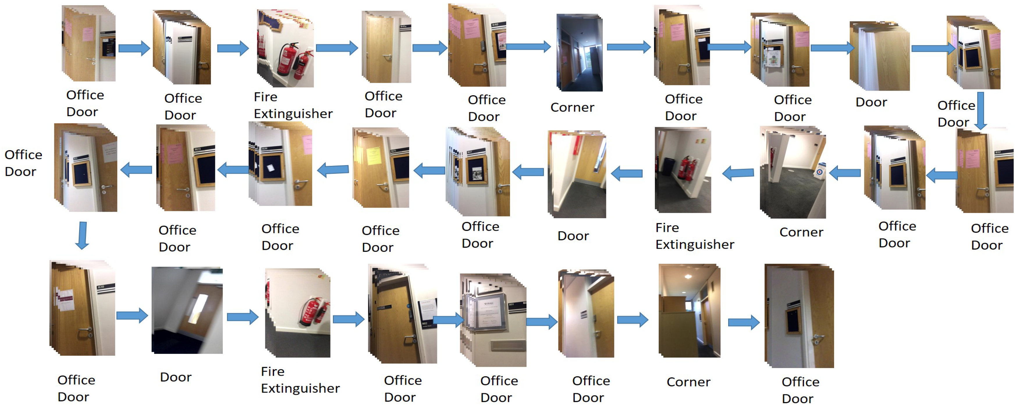
Route 1: The route begins at Node 43 and goes through 28 landmarks, ending at Node 47.
Route 2: The route starts from Node 44 and turns left at all four turns before ending at Node 46. There are 16 landmarks in this route.
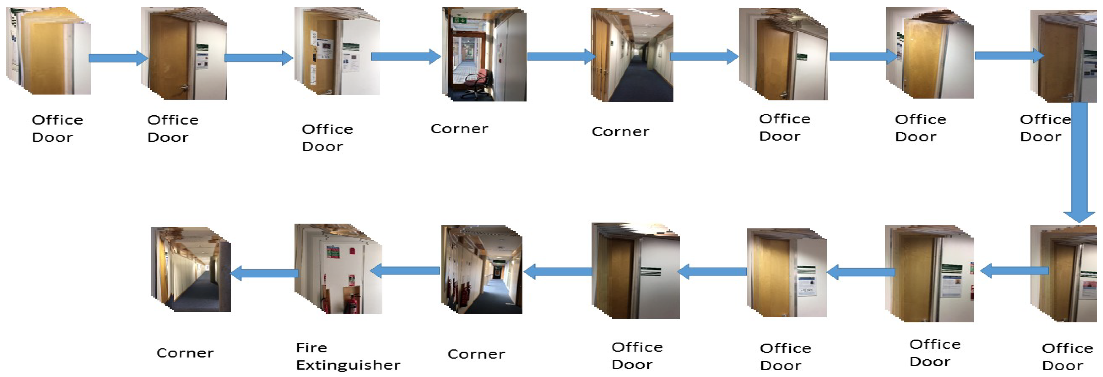
Route 3: This route goes through 15 landmarks. It starts from an office door (Node 52) and ends in the intersection (Node 14). It walks through a sequence of office doors, containing a corner and a left turn.
Route 4: The route starts from the left stair and goes straight to the end corner of the corridor. In total, 10 landmarks are included in this route.
Route 5: This route contains 14 landmarks. It begins from an intersection (Node 16), goes through a sequence of office doors, turns, and elevators, and finally reaches the left stairs.
Route 6: This route starts from a turn (Node 16) and ends at an office (Node 65), going through three turns, containing 17 landmarks.
Route 7: The route begins from a turn (Node 16) and goes to the end of the corner before turning left. It goes straight until reaching the turn (Node 19). It goes down to the turn (Node 17). There are 22 landmarks in this route.
6.2. Landmark Detection
6.2.1. Indoor Object Recognition
The selected landmarks are comprised of nine classes of indoor objects, including eight classes of indoor objects—door (DR), women’s toilet tag (WMTT), men’s toilet tag (MTT), disabled toilet tag (DTT), fire extinguisher (FE), door plate (DP), elevator (ELV), and stairs (ST)—and one class of scene object (corner or intersection) (CN). Together, they form 8 types of landmarks. We also introduce background as a type of class during the training process, which are uninteresting objects (walls mostly). Uninteresting objects act as negative training samples. This increases the discrimination and generalization ability of the classifier.
We collected about 1300 images containing these 10 types of indoor objects (9 of them are objects of interest and 1 is background). About 1000 of them were used for training (fine-tuning the CNN pre-trained on ImageNet data) and the rest for testing. The distribution of the training and testing datasets are shown in Table 1. These data came from two sources, images on the Internet and video frames from the collected data. We leveraged images from the Internet for two reasons. Firstly, the training dataset could be enlarged and thus the discriminative capacity of the trained classifier over the targeted indoor object was improved. Another reason is that our detector can be used in a new environment without retraining.
We selected AlexNet as the basic network and fine-tuned it for our application. The output layer was modified by changing the number of neurons from 1000 to 10. Its parameters were initialized with a normal Gaussian distribution. The other layers were initialized with weights that won the Visual Recognition Challenge in 2012. Parameters of the convolutional layers and fully connected layers were kept fixed and only the parameter of the output layer were learned during the training phase. The CNN was implemented using the Caffe framework [49]. The learning rate was 0.05, and the maximum iteration was 40,000. The network was trained in an MSI laptop in GPU mode. The laptop features a Windows 10 operating system and the processor is Intel i7, and the laptop is fitted with 8 GB of RAM. The graphics processing unit is an Nvidia GTX970M.
We further compare the proposed landmark detection method with traditional handcrafted feature-based methods. Gist [50] is used to represent the visual objects, and the objects are recognized using SVM-based and ANN-based methods. We report the results with the accuracy and the F1 value. F1 value is a measure of classification accuracy, which takes both precision and recall into consideration. Precision represents the number of correct classification results divided by all positive results returned by the classifier. Recall is the number of correct results divided by all the ground true positive samples. The F1 value ranges from 0 to 1, and the higher the value is, the better the performance. F1 can be computed with Equation (16).
The results show that our method achieves the best results compared to SVM-based and ANN-based methods on both average accuracy and F1 value. For each type of object, our method outperforms the other two in terms of accuracy and F1 value. The SVM-based method failed to recognize the doorplates and toilets tags. The ANN-based method also obtained high accuracy but it tended to classify the wall as other objects. This affects the localization application as it adds non-existing landmarks to the sequence.
6.2.2. Landmark Detection Performance
All videos of seven routes were empirically sampled at the rate of three frames per second. Some examples of the visual landmark sequences are shown in Figure 8 and Figure 9. Sampled images were processed with the selective search algorithm to generate 300 patches. Landmarks were determined from the classification results according to the strategy described in Section 4.2.3.
We applied this trained detector and ANN-based detector to the landmark detection on the 1.9 h indoor mobile phone videos. The SVM-based detector is not used due to its low performance on object detection. The results are shown in Table 4.
Our method correctly detected all landmarks in all routes. The ANN-based detector correctly detected landmarks in Route 2 and Route 3. Some walls were wrongly detected as doors in Routes 3, 5, 6, and 7. This demonstrates that our detector outperforms the detector using handcrafted features. Currently, the proposed method cannot be achieved in real time. The majority of time is spent on landmark detection. Although the average time of classifying an image is short using our convolutional neural network (about 0.012 s on our machine), the average time to process a landmark image is about 7 s. The process is time-consuming for two reasons. Firstly, we choose an effective selective search algorithm to generate patches from landmark images, which costs about 3–4 s to generate reliable patches. Secondly, we feed 300 patches of a landmark image to the network to correctly detect landmarks, which takes an extra 3 s. It should be noted that the detection process can be optimized with the development of object detection technologies in computer vision.
6.3. Localization
6.3.1. Performance
We match the detected landmarks with topological map on two situations: a known start and an unknown start. The ground truth routes and the predicted routes are shown in Figure 10. The red line indicates the ground truth trajectory. The green line represents the predicted trajectory with an unknown start, while the blue line represents the predicted trajectory with a known start. The route start is represented with a node with a cyan edge, and the route end is denoted as a node with a red edge. For Routes 1, 2, 4, 5, and 7, predictions of both known and unknown starts are correctly localized since the blue and green lines are in accordance with the red line. For Routes 3 and 6, the two blue lines are in accordance with the red lines, indicating that they are accurately localized under a known start condition. For the unknown start case, Route 3 has two predictions: one starts from Node 27 and ends at Node 13, and the other one starts from Node 52 and ends at Node 14. The latter is the correct path. Route 6 also has two preditions: one starts from Node 10 and ends at Node 30, and the other one begins at Node 16 and stops at Node 65, the latter of which is correct. This shows that the two routes cannot be localized with current observations and further observations are eventually required to be localized. This problem can be solved with the start positions since all seven routes are correctly localized under a known start condition. The results demonstrate that our method is capable of localizing users accurately with a known start and it also works well in some cases with an unknown start. Compared to the landmark detection, the localization process barely costs time. We spend about 0.043 s on average to localize each route.
We further draw comparisons with the HMM-based method in two situations, and the statistical results are shown in Table 5. The number of possible paths is used to report the comparison result. It is notable that the HMM fails to localize all landmark sequences without a known start and only Route 5 is accurately localized given the start position. In addition, our method outperforms the HMM-based method in seven routes with the same conditions.
6.3.2. Analysis
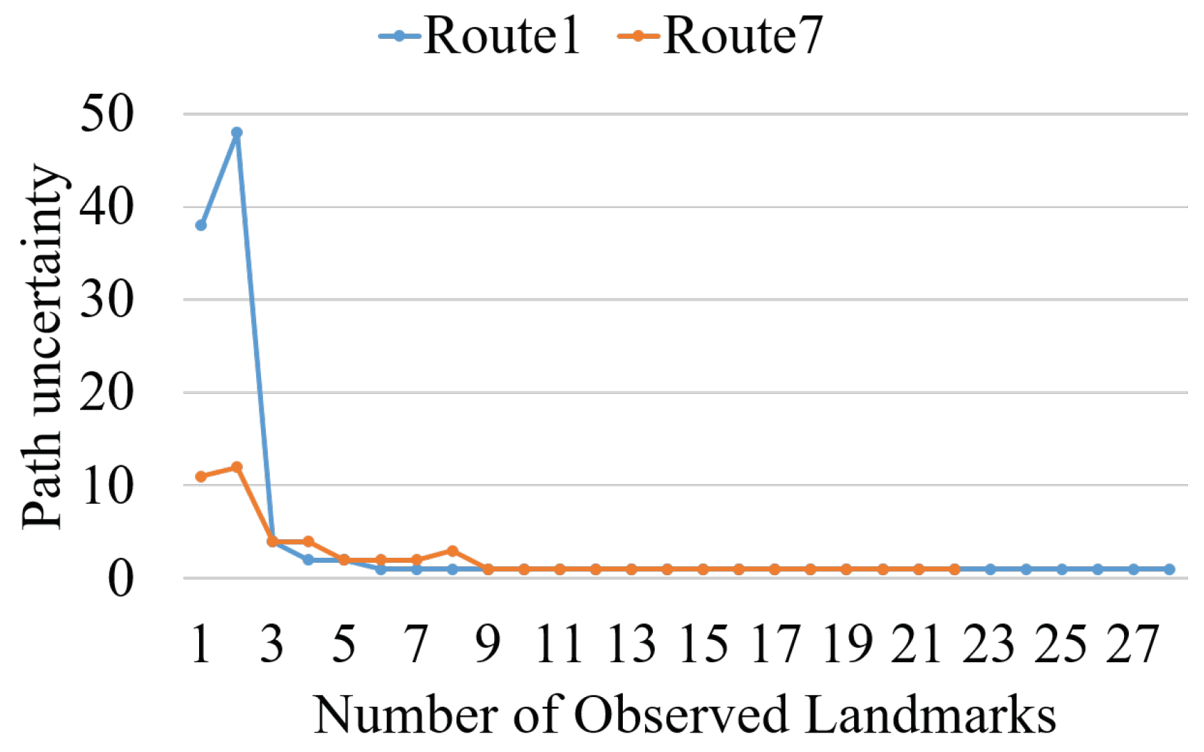
In this section, we evaluated the localization performance of the proposed method regarding the number of observed landmarks. A number of possible paths was used to report performance. We performed experiments in two scenes using Route 1 and Route 7 along with the number of observed landmarks under unknown start conditions. The performance is shown in Figure 11. Route 1 was localized with six landmarks and Route 7 is localized at the ninth landmark. This is because the CSB is more complex compared with the BSB.
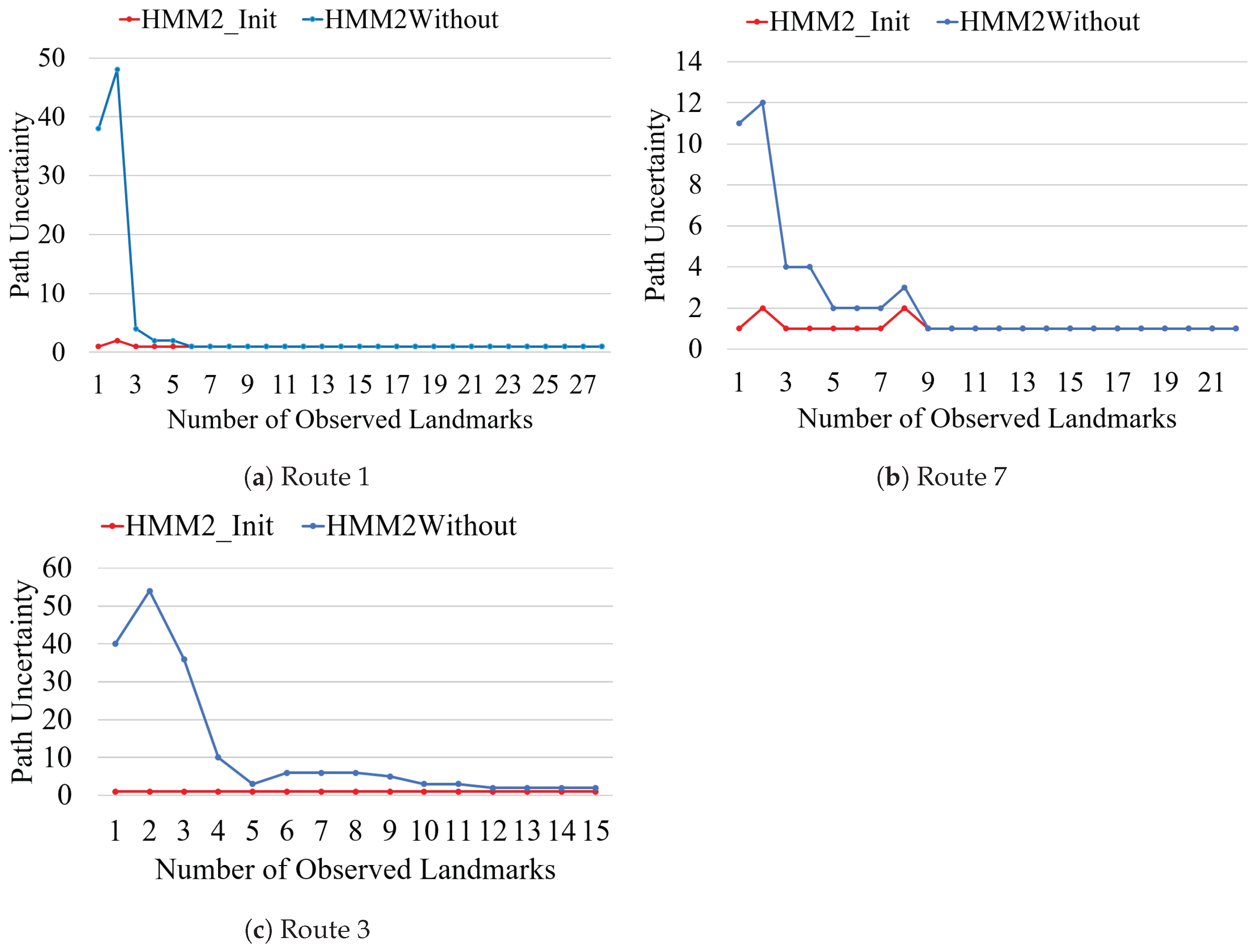
We also conducted experiments to analyze the effects of given route starts regarding the number of observed landmarks. Route 1 from the BSB and Routes 3 and 7 from the CSB were used to perform experiments. It can be seen from Figure 12 that Route 1 is localized from the third landmark with a known start and from the sixth landmark with an unknown start. Route 7 was localized given nine landmarks with an unknown start and three landmarks with a known start. The proposed method was not able to localize Route 3 given unknown starts but localized a route from the second landmark with a known start. This demonstrates that a known start significantly improves the localization performance in two scenes.
7. Conclusions
In this paper, we present a visual landmark sequence-based indoor topological localization method. We propose an innovative representation of landmarks on a topological map, a robust landmark detector, and an effective sequence matching algorithm for localization. Sematic information of stable indoor elements is exploited to represent environmental locations. Compared to the traditional landmark represented by local key point features, combined geometric elements or text information, our representation is able to stay robust facing dynamic environmental change caused by moving pedestrians, illumination, and view changes as well as image blurring. This high-level representation reduces the storage requirement and can be extended to large indoor environments. We present a robust CNN-based landmark detector for landmark detection. Previous landmark detecting methods are devised based on the predefined rules or on color and gradient information. Slight environment changes can significantly influence the landmark detection performance. The background also has a significant influence on detection accuracy. We developed the novel landmark detector using a deep learning technique. Instead of designing the feature with a landmark prior, it learns a deep feature representation for landmarks. Experimental results demonstrate that the previous design feature is confused with the background, while our detector is capable of reliably detecting landmarks from the background.
Our matching algorithm achieves good performance to handle indoor scene ambiguity, as it involves more contextual information. Taking object types as landmark representation saves the storage demand but discards landmark details. This further increases scene ambiguity. Methods depending on feature matching fails to work with the scene ambiguity problem. The HMM helps relieve it to a certain degree but still does not solve it. The experiments show that our methods provide better solutions to the problem than the HMM does.
For future work, we plan to investigate the fusion of low-level visual features with semantic features and with geometric features. This would decrease the scene ambiguity and require fewer landmarks for localization. We also plan to extend the proposed method by utilizing all landmarks in both sides of corridors. The current method adopts side-view capturing, which ignores landmarks on the other side of the corridor and results in the loss of information. Another direction to pursue is the automatic construction of the topological map. Currently, we build our topological map manually based on the floor plan map. When there are no floor plan maps of the scenes, a map needs to be constructed from videos. A localization approach is not able to handle a situation in which a camera stops working for a while as we rely on a landmark occurrence sequence to perform localization. If the camera stops working for a period of time, there will be two video segments. The approach will treat the two video segments as independent videos to perform localization. Two landmark sequences are not able to constrain each other because any number of landmarks and any type of landmarks can be observed during the break.
Author Contributions
Conceptualization, Q.L. (Qing Li) and J.Z.; Data curation, Q.L. (Qing Li), J.G. and G.Q.; Formal analysis, Q.L. (Qing Li), J.Z., B.L. and G.Q.; Funding acquisition, J.Z. and Q.L. (Qingquan Li); Investigation, J.Z. and J.G.; Methodology, Q.L. (Qing Li) and J.Z.; Project administration, Q.L. (Qingquan Li) and G.Q.; Resources, R.C., K.S., T.L. and B.L.; Software, Q.L. (Qing Li) and T.L.; Supervision, J.G., Q.L. (Qingquan Li) and G.Q.; Visualization, R.C., K.S. and B.L.; Writing—original draft, Q.L. (Qing Li) and G.Q.; Writing—review & editing, Q.L. (Qing Li), J.Z., R.C., K.S. and Q.L. (Qingquan Li).
Funding
This work was supported in part by the National Natural Science Foundation of China under Grant 41871329, in part by the Shenzhen Future Industry Development Funding Program under Grant 201607281039561400, in part by the Shenzhen Scientific Research and Development Funding Program under Grant JCYJ20170818092931604, and in part by the Horizon Centre for Doctoral Training at the University of Nottingham (RCUK Grant No. EP/L015463/1).
Acknowledgments
In this section, you can acknowledge any support given which is not covered by the author’s contribution or funding sections. This may include administrative and technical support, or donations in kind (e.g., materials used for experiments).
Conflicts of Interest
The authors declare that there is no conflict of interest.
References
- Ranganathan, P.; Hayet, J.B.; Devy, M.; Hutchinson, S.; Lerasle, F. Topological navigation and qualitative localization for indoor environment using multi-sensory perception. Robot. Auton. Syst. 2002, 41, 137–144. [Google Scholar] [CrossRef]
- Cheng, H.; Chen, H.; Liu, Y. Topological Indoor Localization and Navigation for Autonomous Mobile Robot. IEEE Trans. Autom. Sci. Eng. 2015, 12, 729–738. [Google Scholar] [CrossRef]
- Bradley, D.M.; Patel, R.; Vandapel, N.; Thayer, S.M. Real-time image-based topological localization in large outdoor environments. In Proceedings of the IEEE/RSJ International Conference on Intelligent Robots and Systems, Edmonton, AB, Canada, 2–6 August 2005; pp. 3670–3677. [Google Scholar]
- Becker, C.; Salas, J.; Tokusei, K.; Latombe, J.C. Reliable navigation using landmarks. In Proceedings of the 1995 IEEE International Conference on Robotics and Automation, Nagoya, Japan, 21–27 May 1995; Volume 1, pp. 401–406. [Google Scholar]
- Kosecka, J.; Zhou, L.; Barber, P.; Duric, Z. Qualitative image based localization in indoors environments. In Proceedings of the 2003 IEEE Computer Society Conference on Computer Vision and Pattern Recognition, Madison, WI, USA, 18–20 June 2003; Volume 2, pp. 3–8. [Google Scholar]
- Li, Q.; Zhu, J.; Liu, T.; Garibaldi, J.; Li, Q.; Qiu, G. Visual landmark sequence-based indoor localization. In Proceedings of the 1st Workshop on Artificial Intelligence and Deep Learning for Geographic Knowledge Discovery, Los Angeles, CA, USA, 7–10 November 2017; pp. 14–23. [Google Scholar]
- Ahn, S.J.; Rauh, W.; Recknagel, M. Circular coded landmark for optical 3D-measurement and robot vision. In Proceedings of the 1999 IEEE/RSJ International Conference on Intelligent Robots and Systems, Kyongju, Korea, 17–21 October 1999; Volume 2, pp. 1128–1133. [Google Scholar]
- Jang, G.; Lee, S.; Kweon, I. Color landmark based self-localization for indoor mobile robots. In Proceedings of the 2002 IEEE International Conference on Robotics and Automation, Washington, DC, USA, 11–15 May 2002; Volume 1, pp. 1037–1042. [Google Scholar]
- Basiri, A.; Amirian, P.; Winstanley, A. The use of quick response (qr) codes in landmark-based pedestrian navigation. Int. J. Navig. Obs. 2014, 2014, 897103. [Google Scholar] [CrossRef]
- Briggs, A.J.; Scharstein, D.; Braziunas, D.; Dima, C.; Wall, P. Mobile robot navigation using self-similar landmarks. In Proceedings of the IEEE International Conference on Robotics and Automation, San Francisco, CA, USA, 24–28 April 2000; Volume 2, pp. 1428–1434. [Google Scholar]
- Hayet, J.B.; Lerasle, F.; Devy, M. A visual landmark framework for indoor mobile robot navigation. In Proceedings of the 2002 IEEE International Conference on Robotics and Automation, Washington, DC, USA, 11–15 May 2002; Volume 4, pp. 3942–3947. [Google Scholar]
- Ayala, V.; Hayet, J.B.; Lerasle, F.; Devy, M. Visual localization of a mobile robot in indoor environments using planar landmarks. In Proceedings of the 2000 IEEE/RSJ International Conference on Intelligent Robots and Systems, Takamatsu, Japan, 31 October–5 November 2000; Volume 1, pp. 275–280. [Google Scholar]
- Tian, Y.; Yang, X.; Yi, C.; Arditi, A. Toward a computer vision-based wayfinding aid for blind persons to access unfamiliar indoor environments. Mach. Vis. Appl. 2013, 24, 521–535. [Google Scholar] [CrossRef] [PubMed]
- Chen, K.C.; Tsai, W.H. Vision-based autonomous vehicle guidance for indoor security patrolling by a SIFT-based vehicle-localization technique. IEEE Trans. Veh. Technol. 2010, 59, 3261–3271. [Google Scholar] [CrossRef]
- Bai, Y.; Jia, W.; Zhang, H.; Mao, Z.H.; Sun, M. Landmark-based indoor positioning for visually impaired individuals. In Proceedings of the 2014 12th International Conference on Signal Processing, Hangzhou, China, 19–23 October 2014; pp. 668–671. [Google Scholar]
- Serrão, M.; Rodrigues, J.M.; Rodrigues, J.; du Buf, J.H. Indoor localization and navigation for blind persons using visual landmarks and a GIS. Procedia Comput. Sci. 2012, 14, 65–73. [Google Scholar] [CrossRef]
- Kawaji, H.; Hatada, K.; Yamasaki, T.; Aizawa, K. Image-based indoor positioning system: Fast image matching using omnidirectional panoramic images. In Proceedings of the 1st ACM International Workshop on Multimodal Pervasive Video Analysis, Firenze, Italy, 29 October 2010; pp. 1–4. [Google Scholar]
- Zitová, B.; Flusser, J. Landmark recognition using invariant features. Pattern Recognit. Lett. 1999, 20, 541–547. [Google Scholar] [CrossRef] [Green Version]
- Pinto, A.M.G.; Moreira, A.P.; Costa, P.G. Indoor localization system based on artificial landmarks and monocular vision. TELKOMNIKA Telecommun. Comput. Electron. Control 2012, 10, 609–620. [Google Scholar] [CrossRef]
- Lin, G.; Chen, X. A Robot Indoor Position and Orientation Method based on 2D Barcode Landmark. JCP 2011, 6, 1191–1197. [Google Scholar] [CrossRef]
- Kosmopoulos, D.I.; Chandrinos, K.V. Definition and Extraction of Visual Landmarks for Indoor Robot Navigation; Springer: Berlin/Heidelberg, Germany, 2002; pp. 401–412. [Google Scholar]
- Girshick, R.; Donahue, J.; Darrell, T.; Malik, J. Rich feature hierarchies for accurate object detection and semantic segmentation. In Proceedings of the IEEE Conference on Computer Vision and Pattern Recognition, Columbus, OH, USA, 23–28 June 2014; pp. 580–587. [Google Scholar]
- Zhou, B.; Lapedriza, A.; Xiao, J.; Torralba, A.; Oliva, A. Learning deep features for scene recognition using places database. In Advances in Neural Information Processing Systems; 2014; pp. 487–495. Available online: http://places.csail.mit.edu/places_NIPS14.pdf (accessed on 3 January 2019).
- Werner, M.; Kessel, M.; Marouane, C. Indoor positioning using smartphone camera. In Proceedings of the 2011 International Conference on Indoor Positioning and Indoor Navigation, Guimaraes, Portugal, 21–23 September 2011; pp. 1–6. [Google Scholar]
- Liang, J.Z.; Corso, N.; Turner, E.; Zakhor, A. Image based localization in indoor environments. In Proceedings of the 2013 Fourth International Conference on Computing for Geospatial Research and Application, San Jose, CA, USA, 22–24 July 2013; pp. 70–75. [Google Scholar]
- Chen, C.; Yang, B.; Song, S.; Tian, M.; Li, J.; Dai, W.; Fang, L. Calibrate Multiple Consumer RGB-D Cameras for Low-Cost and Efficient 3D Indoor Mapping. Remote Sens. 2018, 10, 328. [Google Scholar] [CrossRef]
- Zhao, P.; Hu, Q.; Wang, S.; Ai, M.; Mao, Q. Panoramic Image and Three-Axis Laser Scanner Integrated Approach for Indoor 3D Mapping. Remote Sens. 2018, 10, 1269. [Google Scholar] [CrossRef]
- Lu, G.; Kambhamettu, C. Image-based indoor localization system based on 3d sfm model. In IS&T/SPIE Electronic Imaging; International Society for Optics and Photonics, 2014; p. 90250H. Available online: https://www.researchgate.net/publication/269323831_Image-based_indoor_localization_system_ based_on_3D_SfM_model (accessed on 3 January 2019).
- Van Opdenbosch, D.; Schroth, G.; Huitl, R.; Hilsenbeck, S.; Garcea, A.; Steinbach, E. Camera-based indoor positioning using scalable streaming of compressed binary image signatures. In Proceedings of the 2014 IEEE International Conference on Image Processing (ICIP), Paris, France, 27–30 October 2014; pp. 2804–2808. [Google Scholar]
- Hile, H.; Borriello, G. Positioning and orientation in indoor environments using camera phones. IEEE Comput. Gr. Appl. 2008, 28. [Google Scholar] [CrossRef]
- Mulloni, A.; Wagner, D.; Barakonyi, I.; Schmalstieg, D. Indoor positioning and navigation with camera phones. IEEE Pervasive Comput. 2009, 8, 22–31. [Google Scholar] [CrossRef]
- Lu, G.; Yan, Y.; Sebe, N.; Kambhamettu, C. Indoor localization via multi-view images and videos. Comput. Vis. Image Understand. 2017, 161, 145–160. [Google Scholar] [CrossRef]
- Lu, G.; Yan, Y.; Ren, L.; Saponaro, P.; Sebe, N.; Kambhamettu, C. Where am i in the dark: Exploring active transfer learning on the use of indoor localization based on thermal imaging. Neurocomputing 2016, 173, 83–92. [Google Scholar] [CrossRef]
- Piciarelli, C. Visual indoor localization in known environments. IEEE Signal Process. Lett. 2016, 23, 1330–1334. [Google Scholar] [CrossRef]
- Vedadi, F.; Valaee, S. Automatic Visual Fingerprinting for Indoor Image-Based Localization Applications. IEEE Trans. Syst. Man Cybern. Syst. 2017. [Google Scholar] [CrossRef]
- Lee, N.; Kim, C.; Choi, W.; Pyeon, M.; Kim, Y. Development of indoor localization system using a mobile data acquisition platform and BoW image matching. KSCE J. Civ. Eng. 2017, 21, 418–430. [Google Scholar] [CrossRef]
- Chen, Z.; Zou, H.; Jiang, H.; Zhu, Q.; Soh, Y.C.; Xie, L. Fusion of WiFi, smartphone sensors and landmarks using the Kalman filter for indoor localization. Sensors 2015, 15, 715–732. [Google Scholar] [CrossRef]
- Deng, Z.A.; Wang, G.; Qin, D.; Na, Z.; Cui, Y.; Chen, J. Continuous indoor positioning fusing WiFi, smartphone sensors and landmarks. Sensors 2016, 16, 1427. [Google Scholar] [CrossRef]
- Gu, F.; Khoshelham, K.; Shang, J.; Yu, F. Sensory landmarks for indoor localization. In Proceedings of the 2016 Fourth International Conference on Ubiquitous Positioning, Indoor Navigation and Location Based Services (UPINLBS), Shanghai, China, 2–4 November 2016; pp. 201–206. [Google Scholar]
- Millonig, A.; Schechtner, K. Developing landmark-based pedestrian-navigation systems. IEEE Trans. Intell. Transp. Syst. 2007, 8, 43–49. [Google Scholar] [CrossRef]
- Betke, M.; Gurvits, L. Mobile robot localization using landmarks. IEEE Trans. Robot. Autom. 1997, 13, 251–263. [Google Scholar] [CrossRef] [Green Version]
- Boada, B.L.; Blanco, D.; Moreno, L. Symbolic place recognition in voronoi-based maps by using hidden markov models. J. Intell. Robot. Syst. 2004, 39, 173–197. [Google Scholar] [CrossRef]
- Zhou, B.; Li, Q.; Mao, Q.; Tu, W.; Zhang, X. Activity sequence-based indoor pedestrian localization using smartphones. IEEE Trans. Hum.-Mach. Syst. 2015, 45, 562–574. [Google Scholar] [CrossRef]
- Kosecká, J.; Li, F. Vision based topological Markov localization. In Proceedings of the IEEE International Conference on Robotics and Automation, New Orleans, LA, USA, 26 April–1 May 2004; Volume 2, pp. 1481–1486. [Google Scholar]
- Ren, S.; He, K.; Girshick, R.; Sun, J. Faster r-cnn: Towards real-time object detection with region proposal networks. In Advances in Neural Information Processing Systems; 2015; pp. 91–99. Available online: https://arxiv.org/abs/1506.01497 (accessed on 3 January 2019).
- Krizhevsky, A.; Sutskever, I.; Hinton, G.E. Imagenet classification with deep convolutional neural networks. In Advances in Neural Information Processing Systems; 2012; pp. 1097–1105. Available online: https://papers.nips.cc/paper/4824-imagenet-classification-with-deep-convolutional-neural-networks.pdf (accessed on 3 January 2019).
- Uijlings, J.R.; Van De Sande, K.E.; Gevers, T.; Smeulders, A.W. Selective search for object recognition. Int. J. Comput. Vis. 2013, 104, 154–171. [Google Scholar] [CrossRef]
- Thede, S.M.; Harper, M.P. A second-order hidden Markov model for part-of-speech tagging. In Proceedings of the the 37th Annual Meeting of the Association for Computational Linguistics on Computational Linguistics, College Park, MD, USA, 20–26 June 1999; pp. 175–182. [Google Scholar]
- Jia, Y.; Shelhamer, E.; Donahue, J.; Karayev, S.; Long, J.; Girshick, R.; Guadarrama, S.; Darrell, T. Caffe: Convolutional architecture for fast feature embedding. In Proceedings of the 22nd ACM International Conference on Multimedia, Orlando, FL, USA, 3–7 November 2014; pp. 675–678. [Google Scholar]
- Oliva, A.; Torralba, A. Modeling the shape of the scene: A holistic representation of the spatial envelope. Int. J. Comput. Vis. 2001, 42, 145–175. [Google Scholar] [CrossRef]
Figure 1.
(a) Topological map of an indoor space, where there are seven locations. (b) In each of the locations of the space, there is a landmark representing it. Landmarks of the same color are identical (e.g., office doors). A person can only walk from one location to the next linked by a path.
Figure 1.
(a) Topological map of an indoor space, where there are seven locations. (b) In each of the locations of the space, there is a landmark representing it. Landmarks of the same color are identical (e.g., office doors). A person can only walk from one location to the next linked by a path.

Figure 2.
Flowchart of indoor landmark detection.

Figure 3.
Common indoor objects and locations of interest.

Figure 4.
A floor plan map of the B floor in the Business South building (BSB).

Figure 5.
A floor plan map of the B floor in the School of Computer Science building (CSB).

Figure 6.
A landmark topological map of the B floor in the BSB.

Figure 7.
A landmark topological map of the B floor in the CSB.

Figure 8.
Landmark sequence example of Route 1.

Figure 9.
Landmark sequence example of Route 3.

Figure 10.
The localization results of seven routes.


Figure 11.
Localization performance with the number of observed landmarks in two scenes.

Figure 12.
Influence of a known start on localization results.


Table 1.
Distribution of training and testing data.
| Type | CN | DTT | DR | DP | ELV | FE | MTT | ST | WLL | WMTT |
|---|---|---|---|---|---|---|---|---|---|---|
| Training | 56 | 60 | 155 | 63 | 60 | 250 | 58 | 113 | 104 | 55 |
| Testing | 29 | 25 | 33 | 22 | 23 | 36 | 24 | 37 | 31 | 20 |
Table 2.
Indoor object recognition in terms of accuracy.
| Methods | CN | DTT | DR | DP | ELV | FE | MTT | ST | WLL | WMTT | Overall |
|---|---|---|---|---|---|---|---|---|---|---|---|
| SVM | 17.2% | 64.0% | 90.9% | 68.2% | 0.0% | 100% | 0.0% | 56.8% | 3.2% | 0.0% | 44.3% |
| ANN | 82.8% | 80.0% | 97.0% | 86.4% | 73.9% | 97.2% | 87.5% | 70.3% | 61.3% | 80.0% | 81.8% |
| Ours | 100% | 96.0% | 100% | 95.5% | 95.7% | 100% | 100% | 100% | 100% | 95.0% | 98.6% |
Table 3.
Indoor objects recognition in terms of F1 value.
| Methods | CN | DTT | DR | DP | ELV | FE | MTT | ST | WLL | WMTT | AVERAGE |
|---|---|---|---|---|---|---|---|---|---|---|---|
| SVM | 0.29 | 0.78 | 0.50 | 0.77 | Nan | 0.44 | Nan | 0.67 | 0.06 | Nan | Nan |
| ANN | 0.89 | 0.87 | 0.84 | 0.90 | 0.76 | 0.77 | 0.88 | 0.78 | 0.70 | 0.86 | 0.82 |
| Ours | 1 | 0.96 | 1 | 0.98 | 0.98 | 1 | 1 | 1 | 0.98 | 0.93 | 0.98 |
Table 4.
Landmark detection performance in the real data test.
| Route | Landmarks Counts | ANN | Ours | ||||
|---|---|---|---|---|---|---|---|
| DL | CDL | WDL | DL | CDL | WDL | ||
| 1 | 28 | 30 | 25 | 5 | 28 | 28 | 0 |
| 2 | 16 | 16 | 16 | 0 | 16 | 16 | 0 |
| 3 | 15 | 20 | 15 | 5 | 15 | 15 | 0 |
| 4 | 10 | 10 | 10 | 0 | 10 | 10 | 0 |
| 5 | 14 | 18 | 14 | 4 | 14 | 14 | 0 |
| 6 | 18 | 26 | 18 | 6 | 18 | 18 | 0 |
| 7 | 22 | 29 | 22 | 7 | 22 | 22 | 0 |
Table 5.
A statistical comparison landmark sequence localization results of seven routes.
| Route | HMM | HMM2 | ||
|---|---|---|---|---|
| Without | With | Without | With | |
| 1 | 18 | 9 | 1 | 1 |
| 2 | 8 | 2 | 1 | 1 |
| 3 | 1137 | 82 | 2 | 1 |
| 4 | 2 | 2 | 1 | 1 |
| 5 | 12 | 1 | 1 | 1 |
| 6 | 18,346 | 5556 | 2 | 1 |
| 7 | 4 | 2 | 1 | 1 |
© 2019 by the authors. Licensee MDPI, Basel, Switzerland. This article is an open access article distributed under the terms and conditions of the Creative Commons Attribution (CC BY) license (http://creativecommons.org/licenses/by/4.0/).
Share and Cite
MDPI and ACS Style
Zhu, J.; Li, Q.; Cao, R.; Sun, K.; Liu, T.; Garibaldi, J.M.; Li, Q.; Liu, B.; Qiu, G. Indoor Topological Localization Using a Visual Landmark Sequence. Remote Sens. 2019, 11, 73. https://0-doi-org.brum.beds.ac.uk/10.3390/rs11010073
AMA Style
Zhu J, Li Q, Cao R, Sun K, Liu T, Garibaldi JM, Li Q, Liu B, Qiu G. Indoor Topological Localization Using a Visual Landmark Sequence. Remote Sensing. 2019; 11(1):73. https://0-doi-org.brum.beds.ac.uk/10.3390/rs11010073
Chicago/Turabian StyleZhu, Jiasong, Qing Li, Rui Cao, Ke Sun, Tao Liu, Jonathan M. Garibaldi, Qingquan Li, Bozhi Liu, and Guoping Qiu. 2019. "Indoor Topological Localization Using a Visual Landmark Sequence" Remote Sensing 11, no. 1: 73. https://0-doi-org.brum.beds.ac.uk/10.3390/rs11010073
Note that from the first issue of 2016, this journal uses article numbers instead of page numbers. See further details here.