Detection of Glacier Calving Margins with Convolutional Neural Networks: A Case Study


1
Earth System Science, University of California, Irvine, CA 92617, USA
2
Jet Propulsion Laboratory, Pasadena, CA 91109, USA
*
Author to whom correspondence should be addressed.
Remote Sens. 2019, 11(1), 74; https://0-doi-org.brum.beds.ac.uk/10.3390/rs11010074
Submission received: 20 November 2018
/
Revised: 28 December 2018
/
Accepted: 31 December 2018
/
Published: 3 January 2019
Abstract
:The continuous and precise mapping of glacier calving fronts is essential for monitoring and understanding rapid glacier changes in Antarctica and Greenland, which have the potential for significant sea level rise within the current century. This effort has been mostly restricted to the slow and painstaking manual digitalization of the calving front positions in thousands of satellite imagery products. Here, we have developed a machine learning toolkit to automatically detect glacier calving front margins in satellite imagery. The toolkit is based on semantic image segmentation using Convolutional Neural Networks (CNN) with a modified U-Net architecture to isolate the calving fronts from satellite images after having been trained with a dataset of images and their corresponding manually-determined calving fronts. As a case study we train our neural network on a varied set of Landsat images with lowered resolutions from Jakobshavn, Sverdrup, and Kangerlussuaq glaciers, Greenland and test the results on images from Helheim glacier, Greenland to evaluate the performance of the approach. The neural network is able to identify the calving front in new images with a mean deviation of 96.3 m from the true fronts, equivalent to 1.97 pixels on average, while the corresponding error for manually-determined fronts on the same resolution images is 92.5 m (1.89 pixels). We find that the trained neural network significantly outperforms common edge detection techniques, and can be used to continuously map out calving-ice fronts with a variety of data products.
1. Introduction
In recent decades, tidewater glaciers discharging ice from the Greenland Ice Sheet have been thinning, speeding up and retreating inland [1,2,3,4,5,6]. The position of glacier ice fronts reflects a delicate balance of advection and ablation processes [7] and hence is an important proxy for the impacts of regional changes in climate and ocean state on the mass balance in the Greenland Ice Sheet. To assess records of ice front retreat over time, ice front positions are typically manually digitized from aerial imagery [4] or satellite imagery [2,5] using Geographic Information System (GIS) software. Since the launch of Landsat 5 in 1984, the Landsat fleet has captured images of the Greenland Ice Sheet with a repeat cycle of 16 days. However, because the manual ice front digitization process requires a considerable time investment, most current records of calving front retreat are limited to only a few ice front positions per glacier per year, if any. This shortage of data poses a challenge to seasonal analyses of calving glaciers (e.g., [8,9,10,11]), yet seasonal factors may be critical to understanding the pattern of long term retreat of Greenland’s glaciers [12] or to understand for instance the level above which a glacier may be pushed out of balance compared to its state of seasonal, natural variability [6]. In effect, an automated system to rapidly delineate calving front positions would provide a foundation for understanding regional changes on the periphery of the ice sheet over the past several decades, especially with the emergence of a new generation of satellites with high data volume, a high number of acquisitions and higher resolution (e.g., [13,14,15,16]).
Detecting glacier calving fronts in images falls under a more general category of problems that deal with image segmentation. Generally, image segmentation techniques focus on either dividing an image into different regions (e.g., clustering, classification, region extraction) or finding the boundaries between regions (i.e., detection of discontinuities, edge detection). A detailed overview of these categories and techniques is given by [17]. Various techniques have been developed in the past for this class of problems. One of the most prominent of these analytical techniques is the Sobel filter, which uses gradients with a given threshold to detect edges [18]. Other approaches include the “Scale-Space” technique, which, first developed by Witkin et al. [19], detects the desired feature at a coarser scale and tracks it continuously at a higher resolution. This approach was further improved by Perona and Malik [20] by using an anisotropic diffusion process to keep the spatial accuracy of the features and detect edges. Applying these techniques to geophysical images such as ice-covered fjords and geologic formations is challenging due to the noisy nature of the data, variable atmospheric conditions (particularly clouds) and temporal changes on the ground. Seale et al. [3] analyzed the evolution of calving fronts for 32 glaciers in Greenland using a Sobel filter as well as a brightness profiling technique applied to MODIS data. While achieving reasonable results below the resolution of MODIS (0.25 km), this approach relies on the proper selection of subregions around the calving front and heavy use of quality assurance and post-removal of anomalies. Furthermore, analytical techniques relying on brightness gradients in images are dependent on the particular nature of the data. For example, the same gradient thresholds may not be applicable to other instruments and spectral bands. They would also not be applicable to other data types such as radar interferometry (see Massonnet and Feigl [21]). Finally, while this process provides an approximation of overall glacier retreat, it does not yield a digitized-front product which can be used by the glaciological community.
An alternative approach for overcoming these problems is the use of neural networks (see LeCun et al. [22]) that can be trained on any data type to detect glacier fronts. Image segmentation techniques have improved rapidly in recent years due to the progress in deep learning and semantic image segmentation with Convolutional Neural Networks (CNNs) (e.g., see Krizhevsky et al. [23]). Large neural networks with thousands or millions of parameters have allowed much more accurate classification and segmentation of images. In fact, deep neural networks with rectified activation units have already surpassed human performance in some visual recognition tasks (see He et al. [24]).
The issue with such deep neural networks for image segmentation is the need for very large training datasets where the desired features (in this case calving fronts) have already been determined for thousands of images. For many fields of research the shortage of vast training data limits the use of such tools. However, a recent deep neural network architecture developed for biomedical image segmentation, U-Net [25], has been shown to provide highly accurate image segmentation with minimal training data through the use of data augmentation in a deep convolutional neural network. Here we develop a modified version of the U-Net architecture that can identify and extract glacier calving fronts from optical satellite imagery. We discuss our results for a set of glaciers on the Greenland ice sheet. We compare our trained network with the Sobel filter. We conclude on the application of CNN technology to the detection of ice sheet calving margins.
2. Materials and Methods
We detect and reconstruct glacier calving fronts from Landsat imagery with the use of an image segmentation technique that relies on a deep convolutional neural network using a modified U-Net architecture [25]. The methodology is divided into three overarching areas:
- Discussion of raw satellite images, production of training data, and pre-processing of images before training
- Semantic image segmentation and the architecture of the neural network
- Reconstruction of new calving fronts on new data and the post-processing of the outputs of the neural network
Figure 1 summarizes the steps required to pre-process the data, train the network, make predictions, and get the glacier front positions after post-processing. Each of these steps are discussed in the following sections.
2.1. Data and Pre-Processing
We retrieve Level 1 Landsat Data from the USGS Earth Explorer portal for Landsat 5, Landsat 7, and Landsat 8. Calving fronts must be visually discernible in the images in order to be delineated. We mainly rely on L1TP products, but we do use some L1GT/L1GS products as we found the geo-referencing to be sufficient for our purposes. For Landsat 5, we utilize the “green” band (0.52–0.60 m, where ice boundaries appear clearly) with a resolution of 30 m, while for Landsat 7 and 8 we utilize the “panchromatic” band (0.52–0.90 m and 0.503–0.676 m respectively) with a resolution of 15 m. We utilize images from 8 September 1985 to 26 July 2016 for Helheim glacier, 12 July 1994 to 20 October 2002 for Jakobshavn glacier, 3 October 1985 to 5 August 2016 for Kangerlussuaq glacier, and 29 May 1985 to 4 August 2015 for Sverdrup glacier. Furthermore, the seasonal distribution of the images is depicted in Figure S1.1. The scenes are delivered in the UTM projection corresponding to their longitude and latitude to maintain linear and areal distances. We crop the images to the region around the glacier ice front with a buffer of 300 m, an area we define using ice fronts that have previously been digitized manually. SLC-off images may also be used as long as these subset areas of interest are within the unaffected portions of the images.
In order to make it easier for the Neural Network (NN) to detect glacier fronts, we perform a series of pre-processing steps on the input images. Firstly, the cropped input images are mapped onto a rotated uniform grid ( pixels) using cubic interpolation and oriented such that the glacier ice flow is in the y-direction for consistency, in order to improve the performance of the NN across a variety of images. Note that the size of the input images are fixed in the neural network during training. Training the network on different fjord orientations through the use of additional rotation angles would significantly increase training time. Because the total retreat distance varies between glaciers, the scale of the pixel images will also vary. In effect, the resolution of the image subsets are different for each glacier and the approach described herein does not operate on the native resolution of the Landsat products, but rather provides a benchmark for evaluating the performance of different neural network configurations compared to the analytical filter and manual results. The lower resolution images reduce computational resource and training time requirements for our case study. The pixel resolution varies per fjord based on the span of the retreat distance of each glacier over time. The pixel resolutions of the training data are as follows: 61.4 m for Sverdrup, 57.7 m for Kangerlussuaq, and 88.1 m for Jakobshavn. The pixel resolution of the test images on Helheim glacier is 49.0 m. Note that the test data has a slightly higher resolution than the training data, allowing us to test the performance of the NN across resolutions. The location of each fjord and the frames of the input images are shown in Figure S1.2. The corresponding calving front targets, hereinafter referred to as “labels", are manually determined on the original Landsat images and rasterized as single-pixel-thick lines for maximal spatial precision. We also further crop the input images to a size of 150 × 240 pixels with the aim of improving the training time while keeping all the calving fronts within the image frame. Note that this additional cropping is only for faster training and does not have to be applied to the test data. In addition, the architecture of the NN requires the dimensions to be divisible by the number of pooling steps described in the next section. With three pooling layers, the images are padded to be divisible by 8 (see Figure 2), resulting in images.
Furthermore, we apply a series of alterations to the images to make the input more suitable for training the neural network. After a series of experiments with high-pass and low-pass filters, changes of contrast, and application of preliminary edge-detection algorithms, we find the following pre-processing steps provide datasets with consistent and interpretable features for training of the NN, which lead to the best delineation results provided that the same steps are applied to the test data: First, we normalize the image contrasts such that the darkest and lightest points in every image are black and white, respectively. Next we equalize the gray-scale intensities to create a uniform distribution, followed by smoothing and edge-enhancement of the images using the SMOOTH and EDGE ENHANCE operations of the Python Image Library http://www.pythonware.com/products/pil/.
2.2. Semantic Image Segmentation
We develop a Convolutional Neural Network (CNN) [26] with a U-Net architecture [25] with custom sample weights for the segmentation of glacier fronts. U-Net has been very successful for semantic segmentation of biomedical images. It is built based on the architecture of Fully Convolutional Networks (FCN) [27]. The challenge in semantic segmentation is resolving desired features (“what”) and their contextual location (“where”). The idea of FCN is to combine fine, detailed features with coarse, contextual information. U-Net is a modification of such an architecture, which can be conceptualized as having two main components: (1) A “down” component that uses convolutional layers to detect desired features in images in progressively smaller layers with higher numbers of filters or “feature channels”, and (2) An “up” component that has up-sampling layers to convey contextual information to higher resolution layers and reconstruct output images through convolutional layers. These components are labelled in the architecture of our neural network depicted in Figure 2. Convolutional layers consist of a series of kernels that are convolved across the input, mapping each group of pixels into single values in a new layer. These kernels act as filters that map out particular features from the image (such as features associated with glacier fronts). See LeCun et al. [22] for a discussion of convolutional neural networks. Convolutions are represented by red, purple, or gray arrows, as discussed in the following paragraph. During the “down" component, pooling layers are applied to downsample the output of each set of convolutional layers [22]. Pooling is represented by blue arrows in the figure. This dimensionality reduction is a way of introducing location-invariance by combining similar features and coarsening the output of the convolutional kernels. In our neural network we use max-pooling layers, which take the maximum value between each group of 4 pixels, resulting in location invariance within local batches and faster convergence of the network [28]. In the second stage, the images are upsampled by doubling the rows and columns of the previous layer by repeating the rows and columns (represented by cyan arrows) and concatenated with the last convolutional layer with the same dimensions as the upsampled image (yellow arrows). Thus, the detailed global features in the last convolutional layer are combined with the contextual information of the previous layer. This combined upsampled layer is then fed to convolutional layers, as before. The reconstructed image by the last convolutional layer will have the same size as the input images and contain the desired segmented features.
The architecture of our neural network is depicted in Figure 2. Our network is composed of 29 total layers, with 3 downsampling steps and 4 sets of convolutional layers going from 32 to 256 feature channels and the corresponding upsampling steps. We apply convolutional layers with padding (such that the output of each convolutional layer has the same image size as the input) and a step size (“stride”) of 1 as the kernel moves across the image. We use Rectified Linear Units (ReLU) [29] as our non-linear activation function, which has been shown to be very successful in convolutional neural networks [22]. In order to apply regularization and avoid over-fitting to training data, we use Dropout layers [30] between convolutional layers with an elimination fraction of 0.2. This randomly drops some units at each iteration from the neural network in order to minimize over-fitting and excessive reliance on individual units. We find that increasing the dropout fraction significantly increases the “noise” (number of false-positives) in our results. The successive operations of ReLU convolutions→Dropout with 0.2 elimination fraction ReLU convolutions are depicted by single red arrows in Figure 2 for succinct graphical representation. Our downsampling is performed by MaxPooling layers with no padding and strides of 2, which are represented by blue arrows. Therefore, at every step the height and width of the layer is reduced by half while the number of convolutional kernels or bands (also known as feature channels) doubles. The same convolution→dropout→convolution architecture (red arrows) is used in the upsampling stage, where the number of feature channels is halved in each iteration. The upsampling is done by repeating the rows and columns of the previous layer (cyan arrow), and concatenating the resulting matrix with the corresponding higher-resolution layer (yellow arrow). We get performance improvements by also adding a final ReLU convolution to go from the final 32 channels to 3 (represented by a purple arrow), followed by a convolutional layer with a Sigmoid activation function (gray arrow) to get the final reconstructed image. The reconstructed image is flattened into a 36,480 vector for the implementation of pixel-by-pixel sample weights during training, discussed below, which is represented by a black arrow in the final layer in Figure 2. The architecture of the network is also summarized in Table S1.
We use a binary cross-entropy loss function (see Mannor et al. [31]) with custom sample weights for each input image. Note that images of glacier fronts pose a severe class imbalance problem, since the vast majority of pixels are not calving fronts. As a result, the NN learns to obtain high accuracy by simply classifying every pixel as not being part of the calving front. To avoid this false-negative classification artifact, we develop custom sample weights such that for every training example the pixels containing calving fronts have much higher penalties in the loss function if misidentified. In order to have an equal contribution from each class of pixels, the weight is determined as the average ratio of the number of non-boundary pixels to pixels including glacier front boundaries, which is 241.15 in our training set with 123 input images with dimensions . Note that while the weight is distributed individually for each training instance based on the position of the calving front, the value of the weight reflects the class imbalance of the training data in its entirety and is a constant value for all pixels located on calving fronts. We also take advantage of data augmentation by mirroring the horizontal orientation of glaciers (i.e., flipping the images from left to right) to provide different fjord geometries and inverting the grayscale intensities to mimic different shadows. However, we get accurate results even without the use of augmentation, which speeds up the training process (discussed in the next section).
2.3. Post-Processing
To retrieve the geo-located ice front position from the output of the NN, we restore the padding and cropping of the images to the original 200 × 300 pixel size and identify the ocean/glacier area using pre-defined boundaries which delineate the fjord walls. These were obtained by digitizing the fjord boundaries in the same manner as the digitized “true labels”. Note that these lines correspond only to the lateral boundaries of the fjords (i.e., independent of the calving front positions) and therefore only need to be defined once per glacier and may be used for all additional fronts obtained via the NN. We iterate through pairs of pixels on the fjord boundaries to find a least-cost path through the array, where the weights of each “step” are given by the output of the NN. A 500 m buffer is used from the fjord walls. The extracted path of pixels with the least weight is identified as the ice front, and converted to the geographical coordinates of the original clipped Landsat scene used to generate the subset. The geographical coordinates are stored as both raster data and shapefiles which may be used in Geographic Information System (GIS) software.
3. Results
We train the neural network on a set of 123 preprocessed input images from Jakobshavn, Sverdrup, and Kangerlussuaq glaciers. Note that while this may seem like a limited number of training instances, one of the advantages of the utilized network architecture used in this study is its ability to perform well with an extremely limited set of training data. In fact, the U-Net architecture used by Ronneberger et al. [25] used a training set that consisted of 30 pixel images. Training success with few training images is in part enabled by data augmentation, which plays an important role in reducing our output errors, as discussed below. We leave aside 10% of the images chosen randomly during training for cross-validation. The validation dataset is used to prevent overfitting. The training is halted when the validation loss starts to increase as a result of overfitting. In addition, in order to test the ability of the neural network to predict calving fronts beyond the training set for different glacier geometries, we test the trained network on images of Helheim glacier, whose geometry is unknown to the NN during training. Note that this test dataset is in addition to the cross-validation data used during training. We minimize the custom-weighted binary cross-entropy loss function discussed in Section 2 using the Adam optimizer [32] with batches of 10 images at a time. Furthermore, we use a variable learning rate, which is reduced by half after every 5 epochs without any improvements to the accuracy. We test the performance of a variety of NN configurations (discussed in the next section) and find that training the NN described in Figure 2 with horizontal mirroring augmentation with batches sizes of 10 leads to excellent agreement between the “generated” and “true” fronts. Training the network for 54 epochs leads to an accuracy of 92.4% in the training set and 93.6% in the validation set, after which the validation loss starts to increase as a result of over-fitting. Figure 3 shows the result of the NN network on a particularly noisy test image.
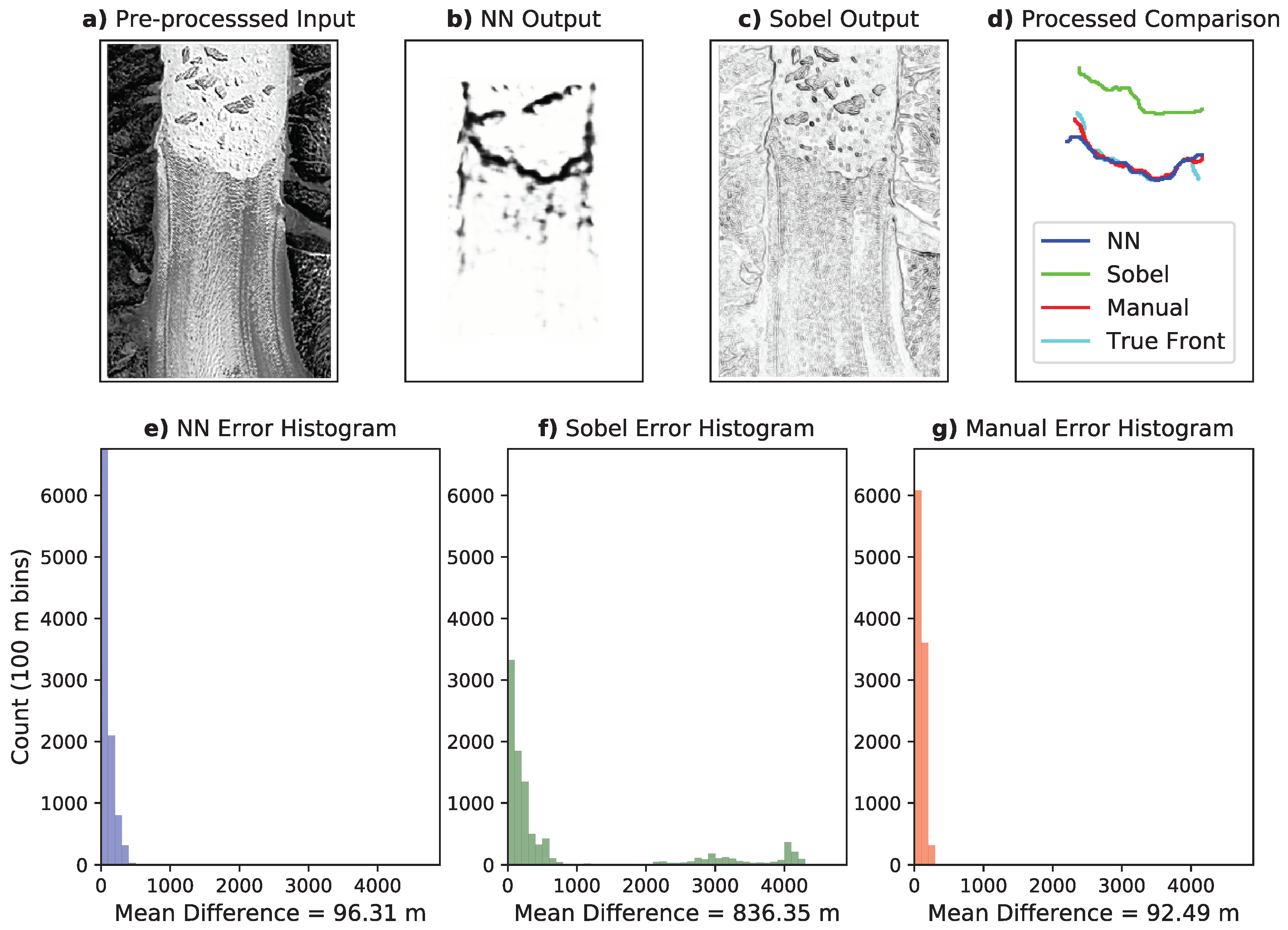
Panel (a) shows the pre-processed input image. Note that we pick this example as an instance of an image that can mislead analytical edge detection filters, but the reported results and errors are drawn from the complete test dataset. The raw output of the NN is shown in Panel (b). It is evident that the neural network is able to extract the calving front from the input image. Figure 3 also compares the output of the NN to the Sobel filter, a common analytic edge detection algorithm that has been used in previous studies (e.g., see Seale et al. [3]). It is clear from Panel (c) that the Sobel filter is very sensitive to noise and identifies many gradients in the texture of the glacier, the icebergs, and the surrounding topography as calving boundaries, which could lead to a false identification of the position of the calving front. Panel (d) shows the extracted fronts in post-processing (as discussed in Section 2.3). Note that we have also included a manually-determined front in addition to the “true” front. While the true front has also been determined manually on the original high resolution (i.e., uninterpolated) geocoded data, the “manual” comparison in Figure 3 refers to hand-drawn fronts on the pre-processed lower resolution rasterized images that are also used for the NN and Sobel processing for an equal comparison of the performances. The neural network performs remarkably well compared with the true boundary. However it is evident that the Sobel filter is not able to extract the calving front as accurately as the NN. Furthermore, the performance of the neural network appears to be comparable to manually-determined front. Results for other test images are provided in the Supplementary Material (Figure S2.1–10).
While Panels (a)–(d) of Figure 3 showcase the output of one image, Panels (e) and (f) show the error analysis obtained from the complete set of test images for the NN, Sobel filter, and manual results. We quantify the errors by breaking the extracted calving fronts of Helheim glacier (which was not used during training) into 1000 smaller line segments and calculating the mean difference between the corresponding segments of the generated and true fronts. Figure 3 shows the distribution of the differences for the NN (e) the Sobel filter (f), and manual results (g). We calculate the total error in the glacier fronts as the mean deviation between all 10,000 line segments in the outputted and true glacier front boundaries. The NN has a mean difference of 96.3 m, equivalent to 1.97 pixels, which is more than 8 times smaller than that of the Sobel filter. The manual output has a mean error of 92.5 m (1.89 pixels), only slightly below the error of the NN. Considering line segments only from the 8 scenes were the Sobel filter is able to successfully delineate the calving front, the errors are 85.3 m (1.74 pixels), 193.0 m (3.94 pixels), and 89.1 m (1.82 pixels) for the NN, Sobel, and manual approaches, respectively. Most of the error in the NN output is attributed to the edges of the calving front, as can be seen in the Supplementary Material. Furthermore, it appears that the Sobel errors have a multimodal distribution. In other words, when the Sobel filter identifies the correct gradient as the calving front, it is in good agreement with the NN results. However, the filter can be easily mislead by other gradients in the image, resulting in a complete mis-identification and large errors for some images, leading to additional peaks in the histogram and larger overall errors. However, even when only the successful Sobel cases are compared, the NN mean error is less than half of that of the Sobel. The manual error histogram shows a more narrow distribution of errors, similar to the NN. The results from the NN, Sobel filter, and the manual technique for individual test images, along with the corresponding errors, can be viewed in the Supplementary Material.
Note that the errors are dependent on the resolution of the input images. As noted before, the resolution of our inputs are less than that of the native Landsat images in order to account for the possible span of ice fronts while minimizing image sizes and training time. However, the errors could be improved further by increasing the resolution and the areal extent of the input images, requiring more computational resources and increased training time. Thus, our benchmark analysis shown above is conducted on the same glacier to limit the influence of resolution and image size on the performance comparison of NN configurations and analytical filter and manual results. We performed the training with the interpolated images on an Intel 2.9 GHz CPU node with 5 Gigabytes of allotted memory. The training took 2 min and 17 s per epoch, resulting in just over two hours of training in total. More computational resources, in particular the use of Graphical Processing Units (GPUs), could result in significant improvements to the training time.
4. Discussion
Images of glacier calving fronts are inherently noisy, with a variety of surfaces and boundaries. Therefore, the application of analytical edge detection schemes such as the Sobel filter [18] results in many false-positive predictions, where any sharp gradients on the surface of the glacier, icebergs, valley walls, and surrounding topography are likely to be labeled as glacier calving fronts. In contrast, a convolutional neural network is able to learn the desired features in the images in order to correctly identify the calving front and mostly ignore other boundaries and sharp gradients. As discussed in Figure 3, the glacier fronts extracted from the output of the NN are in very close agreement to the true front and have similar errors as manually-determined fronts on the same resolution. The analytical filter, however, appears to be very sensitive to noise. It returns noisy images of sharp gradients from which the calving front cannot be correctly extracted in some cases. While customized analytical edge-detection schemes may be able to achieve reasonable results (see Seale et al. [3]), they often rely on dataset-specific parameterizations and thresholds that are not readily applicable to various imagery solutions. The application of neural networks, on the other hand, does not require analytical customization for different datasets. The NN can be trained on any imagery product with the proper training labels. The applicability of NNs for the detection of calving fronts goes beyond optical imagery, and can be potentially applied to other forms of data such as radar, which will be explored in future studies.
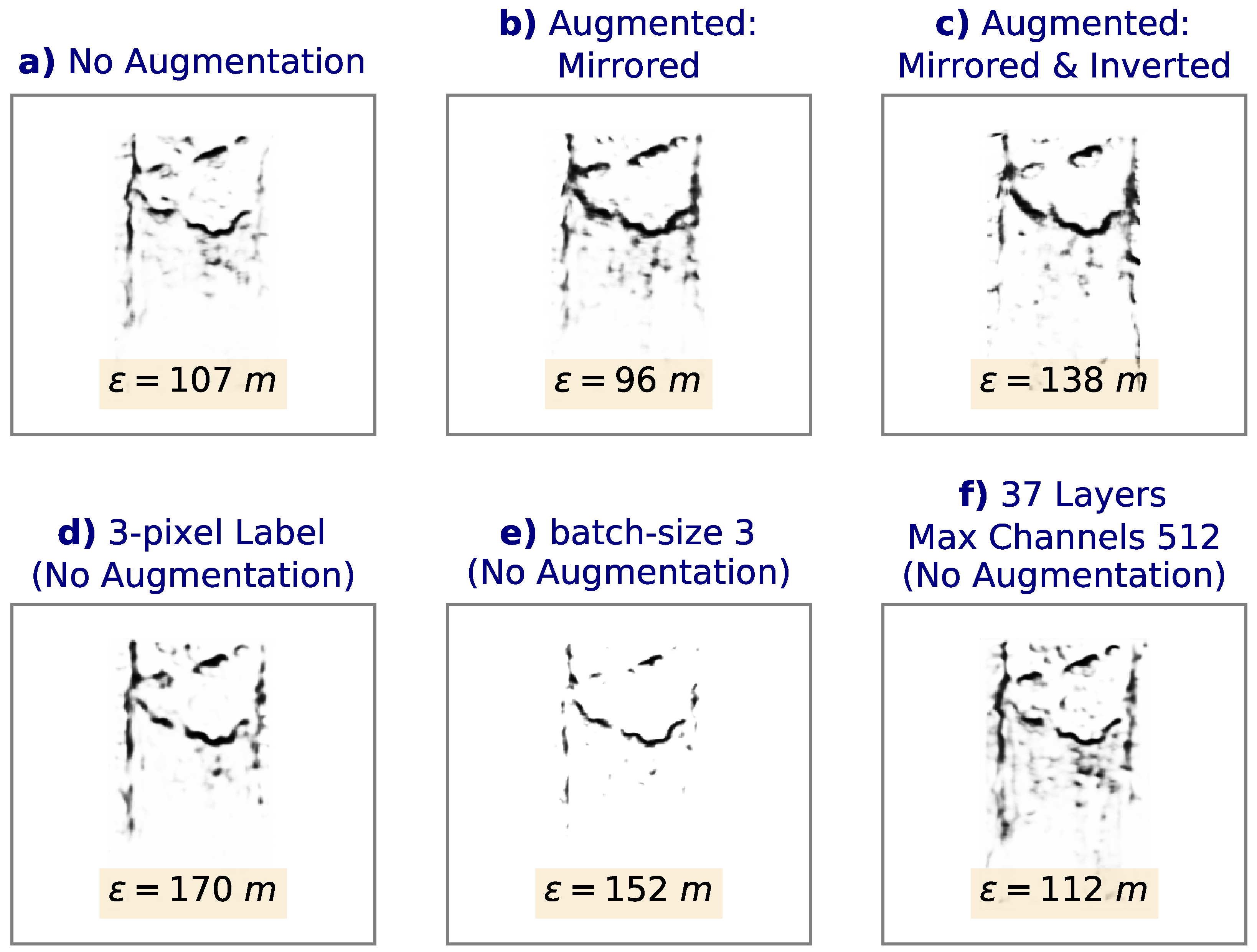
The proper configuration and training of the NN can have a significant effect on the accuracy of the generated calving fronts. Figure 4 showcases various alterations to the NN on the same image used in Figure 3. Panels (a)–(c) use the architecture of the NN shown in Figure 2 without any data augmentation (a), horizontally mirroring the images (b), and horizontally mirroring and inverting the colors of the images (c) during training. We find that data augmentation results in more continuous calving fronts while generally reducing the “noise” (number of false-positives). However, color inversion does not seem to contribute further to the performance of the network. In fact, while horizontal mirroring produces a mean deviation error of 96 m, the addition of inversion increases the error to 138 m. Furthermore, note that data augmentation increases the training time by several fold, depending on the number of alterations. Adding color inversion augmentation increases the training time per epoch from 137 to 217 seconds. As a result, it is desirable to use minimal augmentation while maintaining a low error. Therefore, we restrict the augmentation to horizontal mirroring. Furthermore, Panel (d) shows the effect of increasing the width of the glacier front lines in the training labels from 1 pixel to 3 pixels. While the mean error increases due to the loss of spatial precision, it is interesting to note that the noise, or number of false-positives, also decreases noticeably. This may be a result of the smaller class imbalance and weight ratio in the loss function (which decreases from 241.15 to 82.22), reducing the relative cost for a false classification of the calving fronts compared to background pixels. Therefore, if more pronounced calving front lines with minimal noise are required in post-processing, thicker labels may be desired.
We also find that the number of batches used during training has a significant effect on the results. We use batch sizes of 10 in the chosen NN. On the one hand, using larger batch sizes increases the noise in the output of the neural network, significantly decreasing the accuracy metric in the validation dataset. On the other hand, while using smaller batch sizes reduces the background noise, it also decreases the accuracy, with the mean error changing from 107 m (10 batches) to 152 m (3 batches), as shown in Panel (e). However, smaller batch sizes might be desirable if fewer false-negatives (at the cost of less continuous calving fronts) are required. Note that while smaller batch sizes increase training time per epoch, fewer iterations are required before overfitting in validation loss becomes evident.
Lastly, we also examine the effect of the depth and size of the neural network on the test results. While increasing the depth leads to smaller errors compared to increasing the width or the number of units in each layer (not shown), there are no improvements with respect to the 29-layer NN, as shown in Panel (f). This may be due to the limited availability of training data for a deeper NN. The 37-layer NN (with one more downsample/upsamppling step compared to Figure 2) shows a more noisy output with a mean error of 112 m, slightly larger than the mean error of the corresponding 29-layer output in Panel (a). Note that the same relationship is true with the addition of augmentation. However, in the case of a larger and more varied training dataset, a deeper NN could potentially lead to further improvements.
5. Conclusions
We have used a Convolutional Neural Network (CNN) with a U-Net architecture [25] to automatically detect glacier calving fronts in images obtained from Landsat 5 (“green” band) and Landsat 7 and 8 (“panchromatic” band). After exploring different network architectures and training and augmentation configurations, we find remarkable agreements between the true hand-drawn calving fronts and those obtained by a 29-layer deep neural network with ReLU convolutional layers [29], regularization with 0.2 Dropout layers [30], downsamplinig (MaxPooling [28]) and upsampling layers, a sample-weighted loss function based on the ratio of calving-front vs. non-calving-front pixels, and the utilization of data augmentation. We test the performance of the network not only on new images in the validation dataset, but also on an entirely new glacier with higher spatial resolution to test the effect of different fjord geometries and spatial resolutions on the trained network. After training the NN on Jakobshavn, Sverdrup, and Kangerlussuaq glaciers, we test it on Helheim glacier and obtain a mean deviation error of 96.3 m, equivalent to 1.97 pixels on average, which is comparable to the mean error of 92.5 m obtained from hand-drawn results on the same resolution. As a comparison, the Sobel filter [18], a commonly used analytical edge-detection method (e.g., see Seale et al. [3]) results in a mean error of 836.3 m on the same dataset. Comparing only the successful cases of the Sobel filter, the errors are 85.3 m (1.74 pixels), 193.0 m (3.94 pixels), and 89.1 m (1.82 pixels) for the NN, Sobel, and manual techniques, respectively.
The success of the neural network (NN) in automatically detecting calving fronts, along with the need for a relatively small training set and short training times, makes this approach highly desirable for the continuous monitoring of numerous glaciers around the globe with the ever-growing wealth of remote-sensing data. The use of more spectral bands from various satellites can potentially improve the performance of the NN in the future. Furthermore, unlike analytical edge-detection techniques, the use of neural networks is not limited to optical imagery and can potentially be extended to many data forms such as radar. Therefore, the use of convolutional neural networks in the detection of calving fronts can be a widely applicable and powerful approach for future studies in order to monitor the retreat of numerous glaciers in real time.
Supplementary Materials
The following are available at https://0-www-mdpi-com.brum.beds.ac.uk/2072-4292/11/1/74/s1. The architecture of the NN, the seasonal distribution and locations and frames of the training and testing images, and the generated fronts and the associated errors from the NN, Sobel filter, and manual results for sample test images of Helheim Glacier can be found in the Supplementary Material.
Author Contributions
Y.M. created, trained, and tested various neural network architectures and analytical edge-detection methods, pre-processed the rotated tiles, and wrote most of the manuscript. M.W. provided the input data and the training labels, post-processed the data and geocoded the results, quantified the errors, and wrote some of the manuscript. I.V. and E.R. provided guidance and supervision throughout the project and contributed to the manuscript.
Funding
This research and the APC were funded by a grant from the NASA Cryosphere Program.
Acknowledgments
This work was performed at the University of California, Irvine. Landsat data can be accessed at https://earthexplorer.usgs.gov. The neural network and the trained weights presented in this paper can be accessed at https://github.com/yaramohajerani/FrontLearning.
Conflicts of Interest
The authors declare no conflict of interest. The sponsors of this work had no role in the design of the study; in the collection, analyses, or interpretation of data; in the writing of the manuscript, and in the decision to publish the results.
References
- Howat, I.M.; Joughin, I.; Tulaczyk, S.; Gogineni, S. Rapid retreat and acceleration of Helheim Glacier, east Greenland. Geophys. Res. Lett. 2005, 32. [Google Scholar] [CrossRef] [Green Version]
- Moon, T.; Joughin, I. Changes in ice front position on Greenland’s outlet glaciers from 1992 to 2007. J. Geophys. Res. Earth Surf. 2008, 113. [Google Scholar] [CrossRef]
- Seale, A.; Christoffersen, P.; Mugford, R.I.; O’Leary, M. Ocean forcing of the Greenland Ice Sheet: Calving fronts and patterns of retreat identified by automatic satellite monitoring of eastern outlet glaciers. J. Geophys. Res. Earth Surf. 2011, 116. [Google Scholar] [CrossRef] [Green Version]
- Bjørk, A.A.; Kjær, K.H.; Korsgaard, N.J.; Khan, S.A.; Kjeldsen, K.K.; Andresen, C.S.; Box, J.E.; Larsen, N.K.; Funder, S. An aerial view of 80 years of climate-related glacier fluctuations in southeast Greenland. Nat. Geosci. 2012, 5, 427–432. [Google Scholar] [CrossRef]
- Murray, T.; Scharrer, K.; Selmes, N.; Booth, A.; James, T.; Bevan, S.; Bradley, J.; Cook, S.; Llana, L.C.; Drocourt, Y.; et al. Extensive retreat of Greenland tidewater glaciers, 2000–2010. Arct. Antarct. Alpine Res. 2015, 47, 427–447. [Google Scholar] [CrossRef] [Green Version]
- Wood, M.; Rignot, E.; Fenty, I.; Menemenlis, D.; Millan, R.; Morlighem, M.; Mouginot, J.; Seroussi, H. Ocean-induced melt triggers glacier retreat in Northwest Greenland. Geophys. Res. Lett. 2018, 45, 8334–8342. [Google Scholar] [CrossRef]
- Rignot, E.; Xu, Y.; Menemenlis, D.; Mouginot, J.; Scheuchl, B.; Li, X.; Morlighem, M.; Seroussi, H.; den Broeke, M.v.; Fenty, I.; et al. Modeling of ocean-induced ice melt rates of five west Greenland glaciers over the past two decades. Geophys. Res. Lett. 2016, 43, 6374–6382. [Google Scholar] [CrossRef] [Green Version]
- Schild, K.M.; Hamilton, G.S. Seasonal variations of outlet glacier terminus position in Greenland. J. Glaciol. 2013, 59, 759–770. [Google Scholar] [CrossRef]
- Motyka, R.J.; Cassotto, R.; Truffer, M.; Kjeldsen, K.K.; Van As, D.; Korsgaard, N.J.; Fahnestock, M.; Howat, I.; Langen, P.L.; Mortensen, J.; et al. Asynchronous behavior of outlet glaciers feeding Godthåbsfjord (Nuup Kangerlua) and the triggering of Narsap Sermia’s retreat in SW Greenland. J. Glaciol. 2017, 63, 288–308. [Google Scholar] [CrossRef]
- Catania, G.; Stearns, L.; Sutherland, D.; Fried, M.; Bartholomaus, T.; Morlighem, M.; Shroyer, E.; Nash, J. Geometric controls on tidewater glacier retreat in central western Greenland. J. Geophys. Res. Earth Surf. 2018, 123, 2024–2038. [Google Scholar] [CrossRef]
- Fried, M.; Catania, G.; Stearns, L.; Sutherland, D.; Bartholomaus, T.; Shroyer, E.; Nash, J. Reconciling drivers of seasonal terminus advance and retreat at 13 Central West Greenland tidewater glaciers. J. Geophys. Res. Earth Surf. 2018, 123, 1590–1607. [Google Scholar] [CrossRef]
- Moon, T.; Joughin, I.; Smith, B. Seasonal to multiyear variability of glacier surface velocity, terminus position, and sea ice/ice mélange in northwest Greenland. J. Geophys. Res. Earth Surf. 2015, 120, 818–833. [Google Scholar] [CrossRef] [Green Version]
- Wu, S.; Zhao, T.; Gao, Y.; Cheng, X. Design and implementation of a Cube satellite mission for Antarctic glacier and sea ice observation. Acta Astronaut. 2017, 139, 313–320. [Google Scholar] [CrossRef]
- Roy, D.P.; Wulder, M.; Loveland, T.R.; Woodcock, C.; Allen, R.; Anderson, M.; Helder, D.; Irons, J.; Johnson, D.; Kennedy, R.; et al. Landsat-8: Science and product vision for terrestrial global change research. Remote Sens. Environ. 2014, 145, 154–172. [Google Scholar] [CrossRef] [Green Version]
- Potin, P.; Rosich, B.; Miranda, N.; Grimont, P. Sentinel-1A/-1B Mission Status. In Proceedings of the EUSAR 2018: 12th European Conference on Synthetic Aperture Radar, Aachen, Germany, 4–7 June 2018; pp. 1–5. [Google Scholar]
- Markus, T.; Neumann, T.; Martino, A.; Abdalati, W.; Brunt, K.; Csatho, B.; Farrell, S.; Fricker, H.; Gardner, A.; Harding, D.; et al. The Ice, Cloud, and land Elevation Satellite-2 (ICESat-2): Science requirements, concept, and implementation. Remote Sens. Environ. 2017, 190, 260–273. [Google Scholar] [CrossRef]
- Fu, K.S.; Mui, J. A survey on image segmentation. Pattern Recognit. 1981, 13, 3–16. [Google Scholar] [CrossRef]
- Sobel, I. An isotropic 3 × 3 image gradient operator. In Machine Vision for Three-Dimensional Scenes; Academic Press, Inc.: Orlando, FL, USA, 1990; pp. 376–379. [Google Scholar]
- Witkin, A.; Terzopoulos, D.; Kass, M. Signal matching through scale space. In Readings in Computer Vision; Elsevier: Amsterdam, The Netherlands, 1987; pp. 759–764. [Google Scholar]
- Perona, P.; Malik, J. Scale-space and edge detection using anisotropic diffusion. IEEE Trans. Pattern Anal. Mach. Intell. 1990, 12, 629–639. [Google Scholar] [CrossRef] [Green Version]
- Massonnet, D.; Feigl, K.L. Radar interferometry and its application to changes in the Earth’s surface. Rev. Geophys. 1998, 36, 441–500. [Google Scholar] [CrossRef]
- LeCun, Y.; Bengio, Y.; Hinton, G. Deep learning. Nature 2015, 521, 436. [Google Scholar] [CrossRef]
- Krizhevsky, A.; Sutskever, I.; Hinton, G.E. Imagenet classification with deep convolutional neural networks. In Proceedings of the 25th International Conference on Neural Information Processing Systems, Lake Tahoe, NV, USA, 3–6 December 2012; pp. 1097–1105. [Google Scholar]
- He, K.; Zhang, X.; Ren, S.; Sun, J. Delving deep into rectifiers: Surpassing human-level performance on imagenet classification. In Proceedings of the IEEE International Conference on Computer Vision, Santiago, Chile, 7–13 December 2015; pp. 1026–1034. [Google Scholar]
- Ronneberger, O.; Fischer, P.; Brox, T. U-net: Convolutional networks for biomedical image segmentation. In International Conference on Medical Image Computing and Computer-Assisted Intervention; Springer: Berlin, Germany, 2015; pp. 234–241. [Google Scholar]
- Rawat, W.; Wang, Z. Deep convolutional neural networks for image classification: A comprehensive review. Neural Comput. 2017, 29, 2352–2449. [Google Scholar] [CrossRef]
- Long, J.; Shelhamer, E.; Darrell, T. Fully convolutional networks for semantic segmentation. In Proceedings of the IEEE Conference on Computer Vision and Pattern Recognition, Boston, MA, USA, 7–12 June 2015; pp. 3431–3440. [Google Scholar]
- Nagi, J.; Ducatelle, F.; Di Caro, G.A.; Cireşan, D.; Meier, U.; Giusti, A.; Nagi, F.; Schmidhuber, J.; Gambardella, L.M. Max-pooling convolutional neural networks for vision-based hand gesture recognition. In Proceedings of the 2011 IEEE International Conference on Signal and Image Processing Applications (ICSIPA), Kuala Lumpur, Malaysia, 16–18 November 2011; pp. 342–347. [Google Scholar]
- Nair, V.; Hinton, G.E. Rectified linear units improve restricted boltzmann machines. In Proceedings of the 27th International Conference on Machine Learning (ICML-10), Haifa, Israel, 21–24 June 2010; pp. 807–814. [Google Scholar]
- Srivastava, N.; Hinton, G.; Krizhevsky, A.; Sutskever, I.; Salakhutdinov, R. Dropout: A simple way to prevent neural networks from overfitting. J. Mach. Learn. Res. 2014, 15, 1929–1958. [Google Scholar]
- Mannor, S.; Peleg, D.; Rubinstein, R. The cross entropy method for classification. In Proceedings of the 22nd International Conference on Machine Learning, Bonn, Germany, 7–11 August 2005; pp. 561–568. [Google Scholar]
- Kingma, D.P.; Ba, J. Adam: A method for stochastic optimization. arXiv, 2014; arXiv:1412.6980. [Google Scholar]
Figure 1.
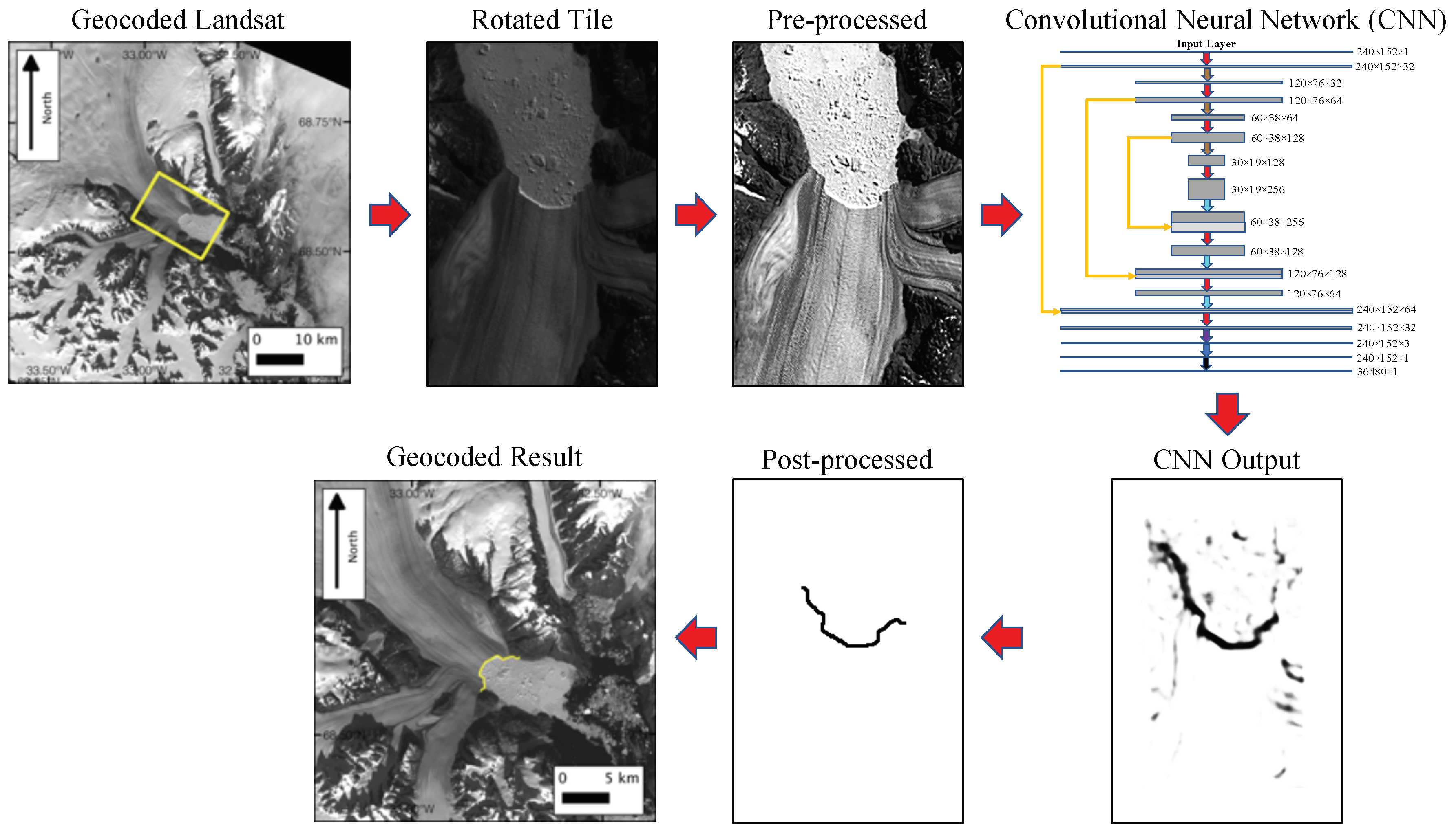
The outline of our methodology: Geocoded Landsat images are trimmed and rotated so that glacier flow is in the y-direction. The images are pre-processed and fed into to a Convolutional Neural Network (CNN) for training (refer to Figure 2 for a zoomed- in version of the CNN panel). The CNN is used to predict new calving front positions, which are post-processed and converted back to geocoded images.
Figure 1.
The outline of our methodology: Geocoded Landsat images are trimmed and rotated so that glacier flow is in the y-direction. The images are pre-processed and fed into to a Convolutional Neural Network (CNN) for training (refer to Figure 2 for a zoomed- in version of the CNN panel). The CNN is used to predict new calving front positions, which are post-processed and converted back to geocoded images.

Figure 2.
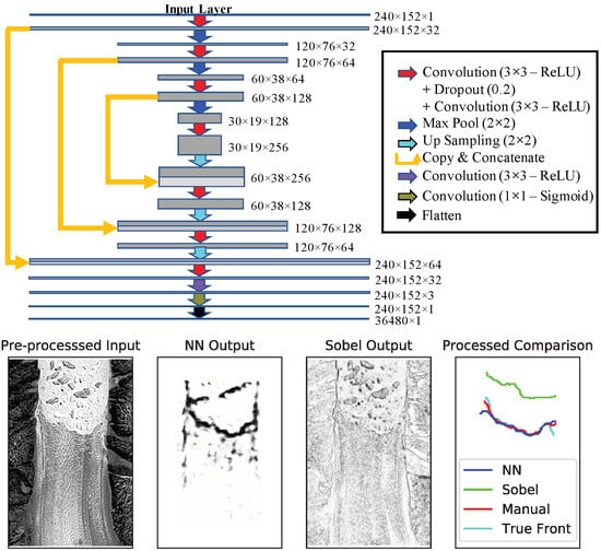
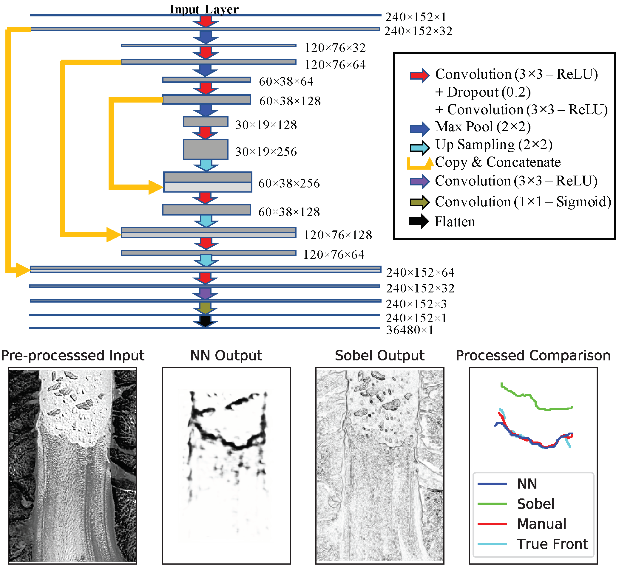
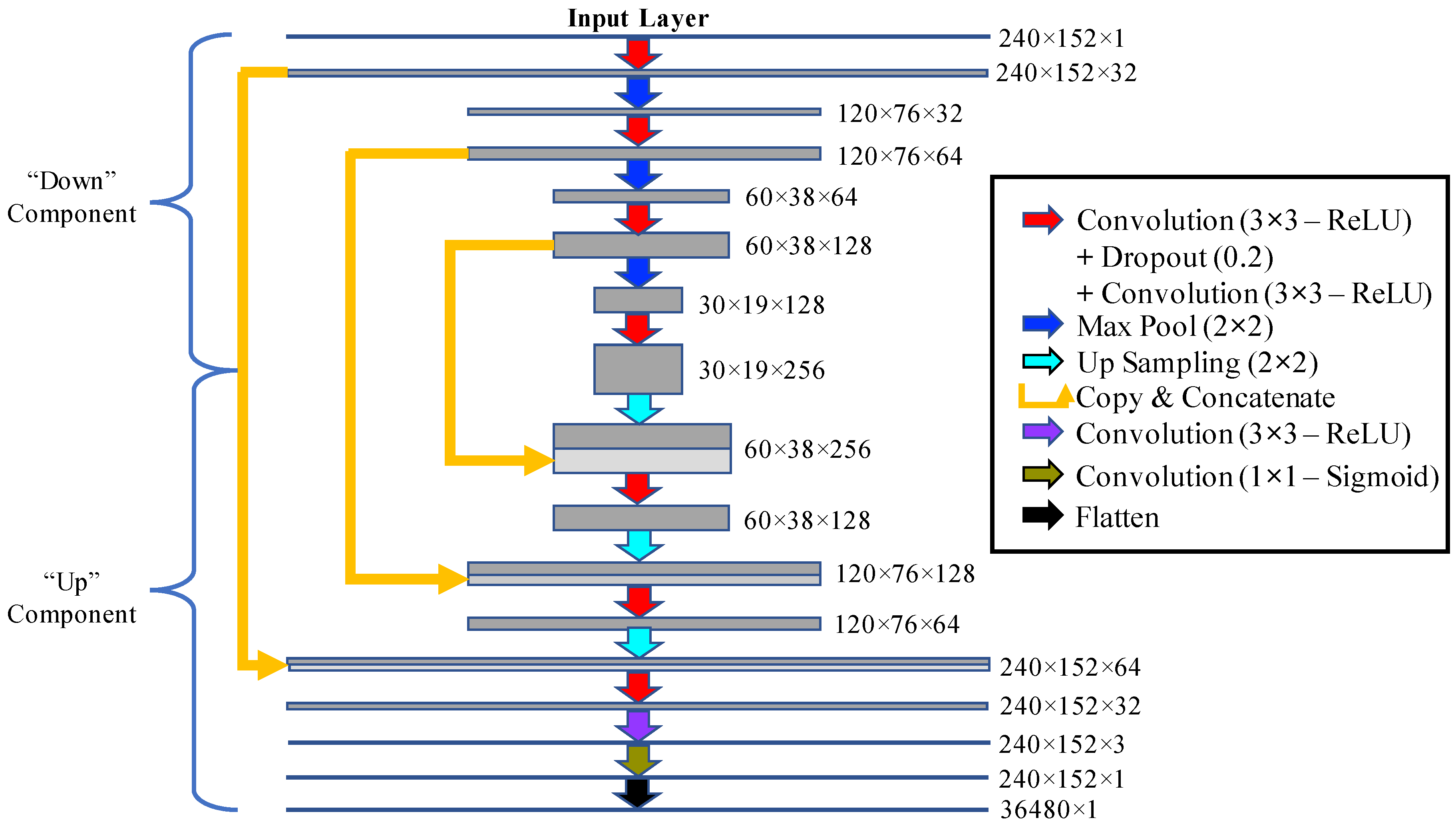
Architecture of the neural network. The length and width of each layer correspond to the pixel dimensions and the number of feature channels (bands) respectively. Convolutional and pooling kernel sizes and upsampling dimensions indicated in parentheses (e.g., for convolutional layers and for pooling). Dropout ratio indicated in parentheses (0.2). The activation function is also stated for convolutional layers (ReLU=REctified Linear Unit, and Sigmoid).
Figure 2.
Architecture of the neural network. The length and width of each layer correspond to the pixel dimensions and the number of feature channels (bands) respectively. Convolutional and pooling kernel sizes and upsampling dimensions indicated in parentheses (e.g., for convolutional layers and for pooling). Dropout ratio indicated in parentheses (0.2). The activation function is also stated for convolutional layers (ReLU=REctified Linear Unit, and Sigmoid).

Figure 3.
The output of the neural network shown for a sample test image of Helheim Glacier from Landsat 5. The pre-processed input image is shown in Panel (a). Panels (b,c) show the raw outputs of the neural network and the Sobel filter, respectively. Panel (d) depicts the corresponding extracted calving fronts compared to the true front, with the addition of the manually-determined front on the same resolution rasterized image used for the NN and Sobel filter. Note that the output of the NN shows remarkable agreement with the true front. Panels (e–g) show the distribution of differences between the generated and true fronts across all test images, with the corresponding mean differences with the true fronts for the NN, Sobel, and manual results, respectively. The NN difference of 96.3 m corresponds to 1.97 pixels. Considering only the 8 of 10 cases where the Sobel filter correctly identifies the calving front, the mean differences for the NN, Sobel, and manual techniques are 85.3 m (1.74 pixels), 193.0 m (3.94 pixels), and 89.1 m (1.82 pixels), respectively.

Figure 4.
A comparison of raw outputs for various architecture and training configurations of the NN (a–f). represents the mean deviation from the true front for each case. Note the best results presented in the Results section correspond to Panel (b).
Figure 4.
A comparison of raw outputs for various architecture and training configurations of the NN (a–f). represents the mean deviation from the true front for each case. Note the best results presented in the Results section correspond to Panel (b).

© 2019 by the authors. Licensee MDPI, Basel, Switzerland. This article is an open access article distributed under the terms and conditions of the Creative Commons Attribution (CC BY) license (http://creativecommons.org/licenses/by/4.0/).
Share and Cite
MDPI and ACS Style
Mohajerani, Y.; Wood, M.; Velicogna, I.; Rignot, E. Detection of Glacier Calving Margins with Convolutional Neural Networks: A Case Study. Remote Sens. 2019, 11, 74. https://0-doi-org.brum.beds.ac.uk/10.3390/rs11010074
AMA Style
Mohajerani Y, Wood M, Velicogna I, Rignot E. Detection of Glacier Calving Margins with Convolutional Neural Networks: A Case Study. Remote Sensing. 2019; 11(1):74. https://0-doi-org.brum.beds.ac.uk/10.3390/rs11010074
Chicago/Turabian StyleMohajerani, Yara, Michael Wood, Isabella Velicogna, and Eric Rignot. 2019. "Detection of Glacier Calving Margins with Convolutional Neural Networks: A Case Study" Remote Sensing 11, no. 1: 74. https://0-doi-org.brum.beds.ac.uk/10.3390/rs11010074
Note that from the first issue of 2016, this journal uses article numbers instead of page numbers. See further details here.