Operational Use of Surfcam Online Streaming Images for Coastal Morphodynamic Studies


1
Instituto Dom Luiz, Faculty of Science, University of Lisbon, Campo Grande, 1749-016 Lisbon, Portugal
2
Geo-Environmental Cartography and Remote Sensing Group, Department of Cartographic Engineering, Geodesy and Photogrammetry, Universitat Politècnica de València, Camí de Vera s/n, 46022 Valencia, Spain
*
Author to whom correspondence should be addressed.
Remote Sens. 2019, 11(1), 78; https://0-doi-org.brum.beds.ac.uk/10.3390/rs11010078
Submission received: 3 December 2018
/
Revised: 24 December 2018
/
Accepted: 28 December 2018
/
Published: 4 January 2019
Abstract
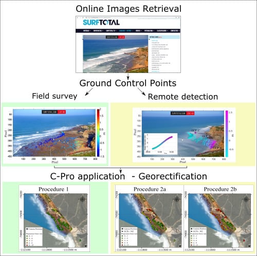
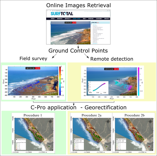
:Coastal video monitoring has been proven to be a valuable shore-based remote-sensing technique to study coastal processes, as it offers the possibility of high-frequency, continuous and autonomous observations of the coastal area. However, the installation of a video systems infrastructure requires economical and technical efforts, along with being often limited by logistical constraints. This study presents methodological approaches to exploit “surfcam” internet streamed images for quantitative scientific studies. Two different methodologies to collect the required ground control points (GCPs), both during fieldwork and using web tools freely available are presented, in order to establish a rigorous geometric connection between terrestrial and image spaces. The application of an image projector tool allowed the estimation of the unknown camera parameters necessary to georectify the online streamed images. Three photogrammetric procedures are shown, distinct both in the design of the computational steps and in number of GCPs available to solve the spatial resection system. Results showed the feasibility of the methodologies to generate accurate rectified planar images, with the best horizontal projection accuracy of 1.3 m compatible with that required for a quantitative analysis of coastal processes. The presented methodologies can turn “surfcam” infrastructures and any online streaming beach cam, into fully remote shore-based observational systems, fostering the use of these freely available images for the study of nearshore morphodynamics.
1. Introduction
The coastal zone is an extremely dynamic environment where the complex interaction between wave action and coastal morphological processes often endanger human occupation and the use of the littoral. Therefore, coastal studies should be as comprehensive as possible, to allow the simultaneous description of both hydrodynamic processes and morphological features, with adequate coverage in spatial and temporal scales. On-ground measurements of nearshore morphology such as bathymetry and beach topography are usually performed by vessel-based or Global Positioning Systems in Real-Time Kinematic (RTK-GPS) [1], respectively. Although these conventional practices provide high spatial resolution measures, their repeatability and thus temporal coverage are limited by their technical, logistical and economical demands [2]. Besides, direct measurements of wave properties (e.g., wave height and wave period) are traditionally obtained by oceanographic devices (e.g., wave gauges, pressure transducers, acoustic doppler current profiler etc.), whose deployment is operationally demanding and difficult, especially at high energy environments with mobile sandy bottoms.
As many nearshore processes have a visible signature on the sea surface, remote sensing has emerged in this context as a valid alternative to provide nearshore measurements. Among numerous remote-sensing methodologies and approaches (e.g., aerial photography, satellite imagery, wave radar, Light Detection And Ranging—LiDAR), shore-based coastal video monitoring has been proved as a cost-efficient and high-quality data collection tool to support coastal scientists and engineers over the last three decades [3].
A video-monitoring station is usually composed of one (or more) video-cameras connected to a personal computer, which has the functions of controlling the optical device and storing the video acquisitions. The optical device is usually installed stable at an elevated position looking at the beach and the nearshore. The pioneer Argus monitoring program [3] was the first scientific program to install a shore-based video monitoring system with the aim of supporting coastal studies through video-derived observations. The Argus system was developed by the Coastal Imaging Lab at the Oregon State University in the early 1990s, and several Argus-based video monitoring stations has been providing coastal image data worldwide ([3] and references therein). To 2003, approximately 30 Argus video-monitoring stations and 120 cameras were operating daily in 8 countries [4]. To date, around 40 Argus stations are still operational on the coasts of three continents.
In the 2000s, the expansion of commercial video systems (e.g., CoastalComs, Erdman) and the development of dedicated image-processing tools (e.g., SIRENA [5], COSMOS [6], Beachkeeper plus [7], ULISES [8]) promoted the installation of video monitoring stations for scientific purpose with the use of relatively cheap internet protocol (IP) video cameras to overcome the expensive installation and purchase of Argus system (e.g., [9]). Although the lower spatial coverage in comparison with other remote-sensing technologies (e.g., satellite imagery, wave radar, LiDAR), shore-based video monitoring technique gives an excellent compromise between spatial and temporal resolutions, beneficial to support both short- and long-term synoptic analysis of the hydro- and morphodynamic processes occurring in the nearshore.
Despite the large exploitation of coastal video stations over last decades, the use of online streaming web-cam for quantitative scientific studies has been weakly investigated. For example, coastal “surfcams” are video cameras installed at the coast with the main aim of remotely providing visual information of beach and sea state to beachgoers and surf users, streaming near-continuous video over the internet. The main objective of this paper is to provide operational procedures for a research-oriented use of surfcam images.
The following Section 1.1 and Section 1.2 present a comprehensive overview of standard video image pre-processing and scientific applications of coastal video monitoring, in order to give a perception of the importance that such a technique has gained in coastal studies over the last decades. Section 1.3 describes the main issues related to the use of surfcams and underlines the specific objectives of this paper, outlining the main methodological steps that are presented.
1.1. Standard Image Rectification Procedure
In order to exploit the images acquired by a coastal video system, an accurate procedure must be applied to raw imagery data to obtain referenced planar images (e.g., [10]). The camera calibration process is the procedure that estimates the intrinsic parameters of camera lens and sensor. The intrinsic camera parameters, also called internal orientation parameters (IOPs), are namely the focal length f, the position of the principal point (uc, vc), and the distortion coefficients of the camera lens kj. Determination of IOPs is necessary to correct the image distortion inducted by the lens curvature. A conventional camera calibration procedure is performed using several screenshots of checkerboard patterns panel taken by the camera with different poses. Freely available toolboxes such as Camera Calibration Toolbox for Matlab [11] can be extensively used to execute this required process and apply the correction to the images (e.g., [9,12]).
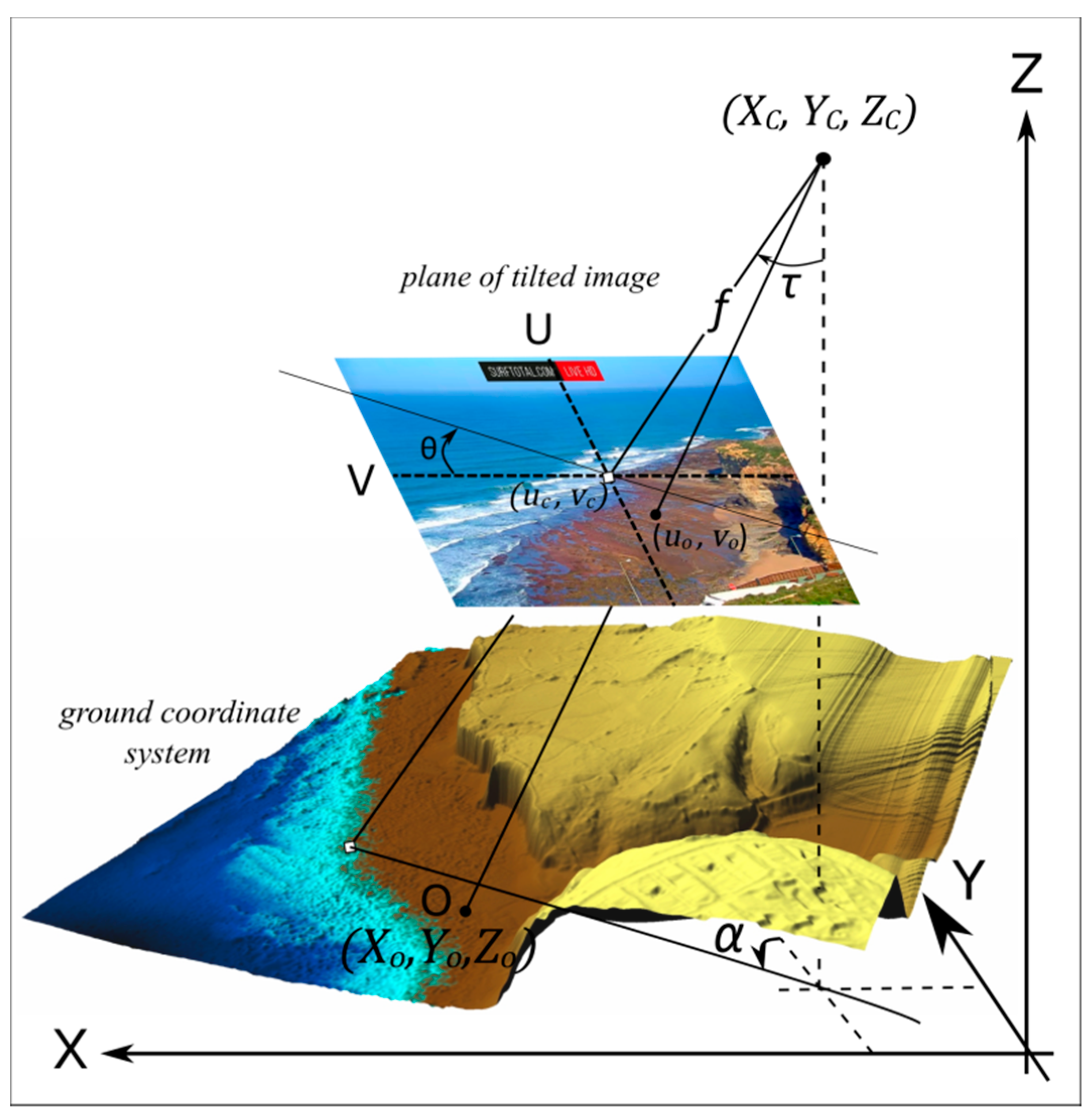
The image rectification procedure transforms an undistorted oblique image into a plan view equivalent image, known as rectified image (e.g., [6]). Given the IOPs computed by the preliminary camera calibration, standard photogrammetric procedures such as the collinearity or the direct linear transformation (DLT) methods (e.g., [10,13]), establish the relation between terrain (X, Y, Z) and image (U, V) spaces by determining the external camera orientation parameters (EOPs), namely the camera position XC, YC, ZC, and orientation (azimuth α; tilt τ, and roll θ). The basis of the spatial resection process follow the classical physical pinhole camera model (Figure 1), which describes the mathematical relationship between the coordinates of a point in the 3D space (XO, YO, ZO) and its projection onto the image plane (uo, vo).
In order to solve the collinearity equation or the DLT equation systems for the spatial resection geometry, it is necessary to identify on the oblique undistorted image a minimum of ground control points (GCPs) whose real-world coordinates are known. In general, a minimum amount of six GCPs is required. GCPs can be selected on fixed structure on the coast (such as breakwaters, houses, paths), can be installed in form of panels visible on the image (e.g., [15]), or can be collected by RTK-GPS survey and later identified on the acquired image sequence. The solution of the equations system allows the transformation of the undistorted image into a planar image map, whose pixels have real-world coordinates.
1.2. Coastal Video Monitoring Applications
Video-based morphodynamic studies uses special images, namely Timex, Variance and Timestack, generated from the acquired and rectified image sequences.
TIMe-EXposure images (Timex) are created by the mathematical average of single image intensity collected over a period of sampling ([3]), usually chosen of 10 min. The averaging of pixel intensity smoothes out variations in wave dissipation and waterline oscillation on the shore, along with filtering out moving objects in the camera’s field of view, such as ships, vehicles and people. The main characteristic of Timex is to underline the preferential location of wave breaking as white bright intensity pattern (e.g., [16]). As submerged sand bars cause preferential breakings over the bar crest, Timex images can be used to find the position and the long-shore development of submerged nearshore sand bars. This property has been exploited for the study of nearshore sand bar migration (e.g., [17,18,19]), rip currents (e.g., [20,21,22,23]), and beach state characteristics (e.g., [24,25,26,27,28]). Since on Timex the swash movements on the foreshore slope are smoothed out, several algorithms have been proposed for shoreline detection on Timex images (e.g., [4,29,30,31]) and have been widely used for a long-term monitoring of shoreline change (e.g., [32,33,34]).
Variance images are created by computing the standard deviation (and despite the name, not the variance) of the individual images which are collected over a period of sampling, as for Timex ([3]). Variance images are bright on the areas with large temporal variability, while unchanged areas appear dark. Thus, a sandy beach is shown as dark in a Variance, while the surf zone appears very bright, due to the pixel intensity variation in relation to breaking waves. Although Argus stations and other video systems have been producing Variance for long time, this kind of images has been seldom used. Few examples of the use of Variance can be seen in Vousdoukas et al. [9], Simarro et al. [35] and Rigos et al. [36], mainly regarding shoreline contour detection.
A third kind of special image, Timestack image, is generated by sampling a single line of pixels from each image over the period of acquisition and concatenating such array of pixel according to the frame acquisition frequency. Timestack is, therefore, composed by pixel intensity time series over a given image sequence. In general, a video data sampling period of 10 min is considered, however the chosen time interval can vary depending on the system set up and/or on the main purposes of the study (e.g., from 7 min to 34 min in Stockdon et al. [37]; and 20 min in Almar et al. [38]). Timestacks were originally produced with the main purpose of studying wave runup process on the foreshore [39,40,41], as the camera acquisitions allowed the monitoring of the high-frequency waterline oscillation on the beach slope. Over the last few decades, Timestack images have been extensively applied to advance in foreshore runup knowledge [42,43,44,45,46,47,48,49,50,51], to improve runup measurements [8,52,53] and to propose new wave runup parameterization [37,54,55,56]. Besides the possibility of measuring wave runup, Lippmann and Holman [57] related Timestack pixel intensity to temporal series of water surface elevation. Exploiting such property, authors measured the wave period applying frequency domain analysis [16,58] or computing wave spectrum [59]. Another Timestack application resides on the measurement of wave celerity [60,61,62,63], which allowed for retrieval of the nearshore subtidal bathymetry through a depth inversion technique [38,64,65,66]. Finally, Timestack images were used to estimate wave breaking height [67,68,69,70], to measure overwash velocity [71], and along-shore Timestacks were adopted to estimate longshore currents [72].
1.3. Surfcam Images
The state of art presented in Section 1.2 emphasizes the capability of a standard coastal video monitoring technique in quantifying a diverse range of important coastal processes. Therefore, it is of interest to explore the opportunities of potentially increasing the coastal imaging acquisition. For instance, two previous studies were conducted to investigate the possibility of using surfcam network for coastal monitoring [73,74]; however, these works were limited to the use of a commercial software for shoreline monitoring and inshore wave measurements [75].
The main purpose of this study is to present practical methodological approaches to rectify surfcam images accurately, in order to exploit online streamed images for scientific studies. The video acquired by a surfcam at the Riberia d’Ilhas beach on the Portuguese coast are used as case study.
The quantitative use of surfcam recreational cameras is mostly limited by their logistic. Most of the installation sites of these devices are not directly accessible, as they are located for instance on rooftop buildings, private houses or streetlights posts. As a consequence, it is often not possible to perform the conventional camera calibration procedure described in Section 1.1, and neither to survey the camera position coordinates. In the context in which standard rectification process cannot be performed, the Coastal Projector monitoring system “C-Pro” [76] offers a valuable computational solution to provide the missing photogrammetric requirements, thus to solve the spatial resection systems for getting precise rectified planar images.
C-Pro adopts the terrestrial horizon visible on an image as a photogrammetric constraint, to incorporate the two equations that describe the horizon inclination in the collinearity system. As working with surfcam images generally implies the lack of knowledge of the IOPs and EOPs, the horizon constraint reduces the number of unknowns in the equations system. In order to achieve an accurate determination of all photogrammetric parameters, C-Pro solves the linearized equations system with the weighted least square method, whose finest solution gives the IOPs and EOPs corrections after an iterative optimization. The minimum amount of required GCPs changes depending on the number of unknowns to be solved by the equations system, given that the incorporation of the horizon equations can also reduce the required number of GCPs.
This paper addresses firstly the GCPs sampling problem. Besides the conventional in-situ collection of GCPs (Section 3.3), we propose a novel method to remotely acquire GCP coordinates and elevation. The synoptic combination of freely-available-online tool and video technique supplies the required points to transform image information into real-world coordinates (Section 3.4). Successively, we tested C-Pro operational capability in retrieving the set of parameters required to perform the image rectification process. Since C-Pro adapts its methodology in accordance with the available input dataset, three analytical procedures are shown (Section 3.6), distinct both in the design of the computational steps and in number of GCPs available to solve the spatial resection system. The analysis of the results focuses on the accuracy achieved by the remote method for GCP collection (Section 4.1) and compares the positional accuracy of rectified planar images generated by C-Pro through the different procedures (Section 4.2 and Section 4.3). A discussion of the advantages and backwards of the proposed solutions associated with surfcam images use and rectification is then presented.
2. Study Site
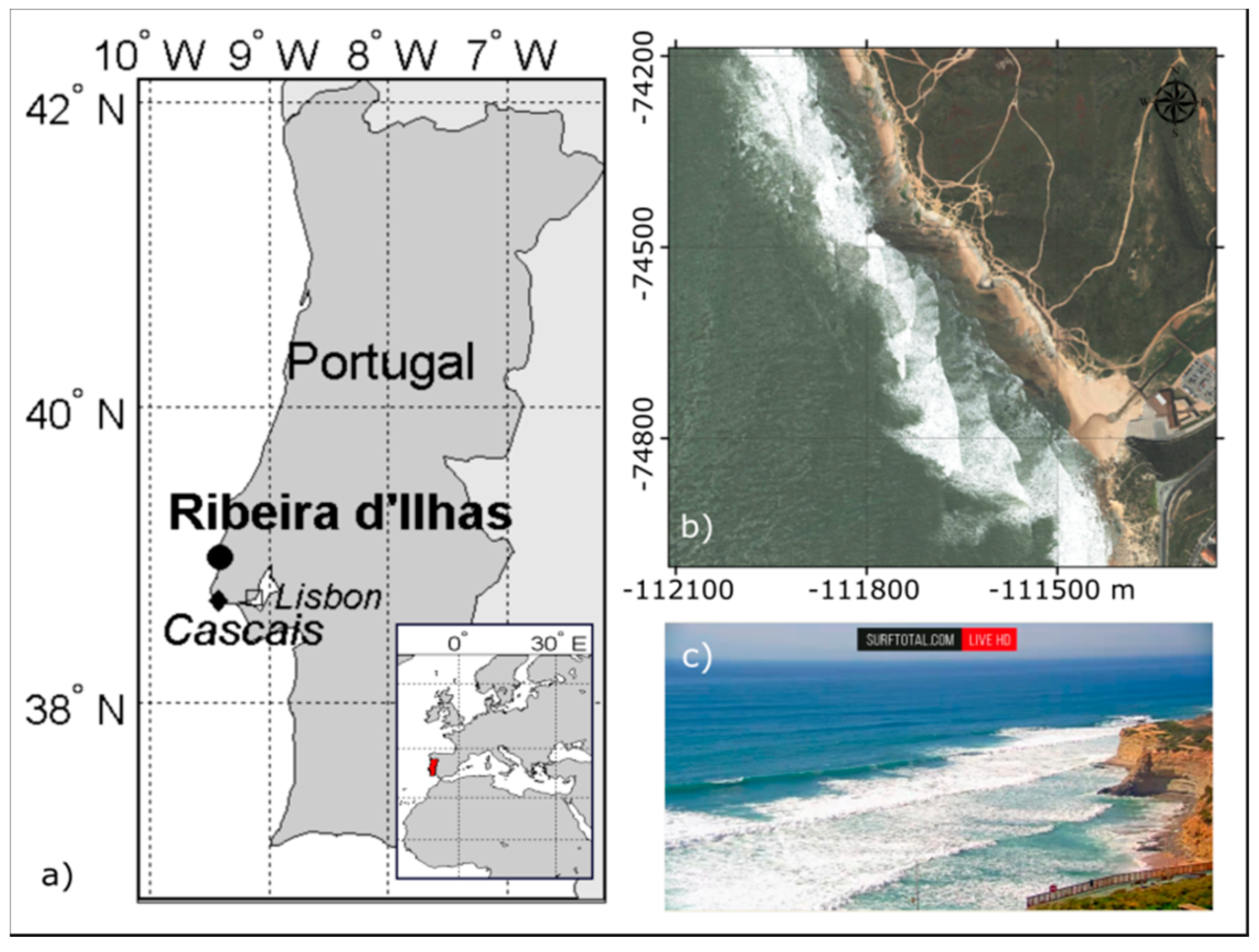
The present work is supported on images acquired at the case study of Ribeira d’Ilhas (38°59′17.0″N, 9°25′10.4″W), a beach that develops over a rocky-shore platform located on the Portuguese western coast, facing the North Atlantic Ocean (Figure 2). The beach extends for about 300 m along-shore, with a NW-SE orientation, and it is limited southwards by a 55 m high cliff and northwards by a small headland. The intertidal shore platform presents a low gradient slope (tanβ = 0.01). This site is a famous stage for many national and international surfing events. The collaboration with the company Surftotal (https://www.surftotal.com/) allowed the use of the images (Figure 2c) acquired by a surfcam installed at the study site.
The video station consisted in a video camera mounted on a house roof at an elevation of about 80 m (mean sea level, MSL) and about 400 m from the shoreline. The camera was installed in a private property which was not accessible. The camera view was set steady looking at the Riberia d’Ilhas shore and nearshore during two days (28 and 29 of March 2017).
3. Methods
This section describes methodological steps to obtain rectified images from raw surfcam video acquisition. The methods differ in the sources used to retrieve the GCP locations, conditioning theirs reliability and number, and in the C-Pro methodological procedures to compute the resection parameters and generate the image planar map.
3.1. Surfcam Case Study
About 18 h of video bursts were retrieved from surfcam acquisition using a password-protected uniform resource locator (URL) web address supplied by Surftotal company. Image frames (800 × 450) were streamed online at a frequency of 15 Hz, however they were extracted from video burst by a dedicated Matlab-based algorithm at a frequency of 5 Hz, to limit data storage space and processing time. From a first visual analysis of the images (Figure 3), the horizon line looked fairly straight, and therefore the distortion inducted by lens curvature were considered negligible in this work. The whole dataset of 380,000 frames was converted in a sequence of 94 10-min Timex images, 52 Timex for the first day of video acquisitions (from 10:00 till 18:30), 42 for the second day (from 11:00 till 18:00). In this work, only the images from the first day of acquisition were used.
3.2. Water Level
Five pressure transducers (PTs) were placed along a cross-shore transect to measure water level and wave properties during the two days of image acquisitions (Figure 3). Four sensors covered a cross-shore length of about 35 m with an offset of around 18 m in the intertidal area. The last sensor was placed at the bottom of the cliff to measure swash properties during high tide. Data were acquired at 2 Hz. Pressure data of the most seaward PT were used as reference for water level η in this work.
Time series of water level was also retrieved by the tide gauge (TG) of Cascais (38.70°N, 9.43°W—Figure 2), available at the web site of the Portuguese General Direction of the Territory [77]. This second dataset represents an alternative remote source for hydrodynamic data available in absence of oceanographic instrumentation in the field.
3.3. Method 1—In-Situ Acquisition of Ground Control Points (GCPs)
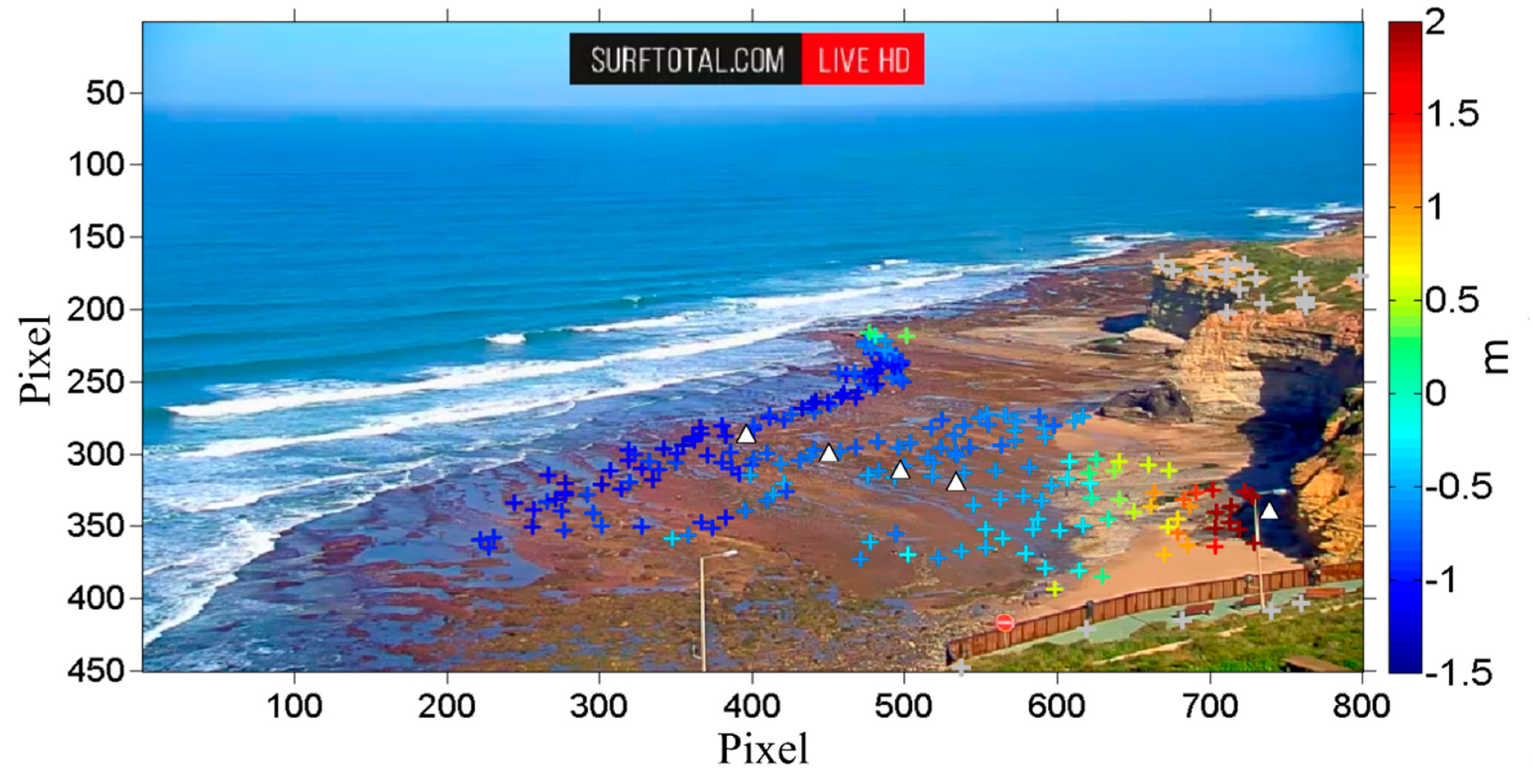
During the first day of image acquisition, an accurate field experiment was conducted using RTK-GPS instrumentation. A large number of points (206) was surveyed in the field of view of the camera, both on the top of the cliff and on the rocky-shore platform. Their elevation ranged between −1.5 m and 53 m (MSL). Successively, these points were manually marked on the oblique surfcam images (Figure 3), navigating through the image sequence and identifying the positions of the operator while acquiring the points with RTK-GPS instrumentation. Among these points, some were chosen as GCPs for solving the geometry of the photo, some other were used as checkpoints for assessing the precision of rectification process (see Section 3.6.1). Hereinafter, we refer to these terrain points collected by the in-situ classical methodology as “Method 1”.
3.4. Method 2—Remote Acquisition of GCPs
Considering that surfcam images can be retrieved online, but the field site might not be easily accessible (e.g., remote site), a second method to remotely retrieve GCPs location was devised, based on the use of the freely available web tool Google Earth. Google Earth is the most popular computer program that renders a 3D representation of Earth based on satellite imagery [78]. In version 5.0, Google Earth introduced Historical Imagery, allowing users to navigate through historical satellite imagery. To date, on Google Earth location corresponding to the study site, images from 13 different dates are available from 2006 to 2016, and could be used to support the acquisition of GCPs.
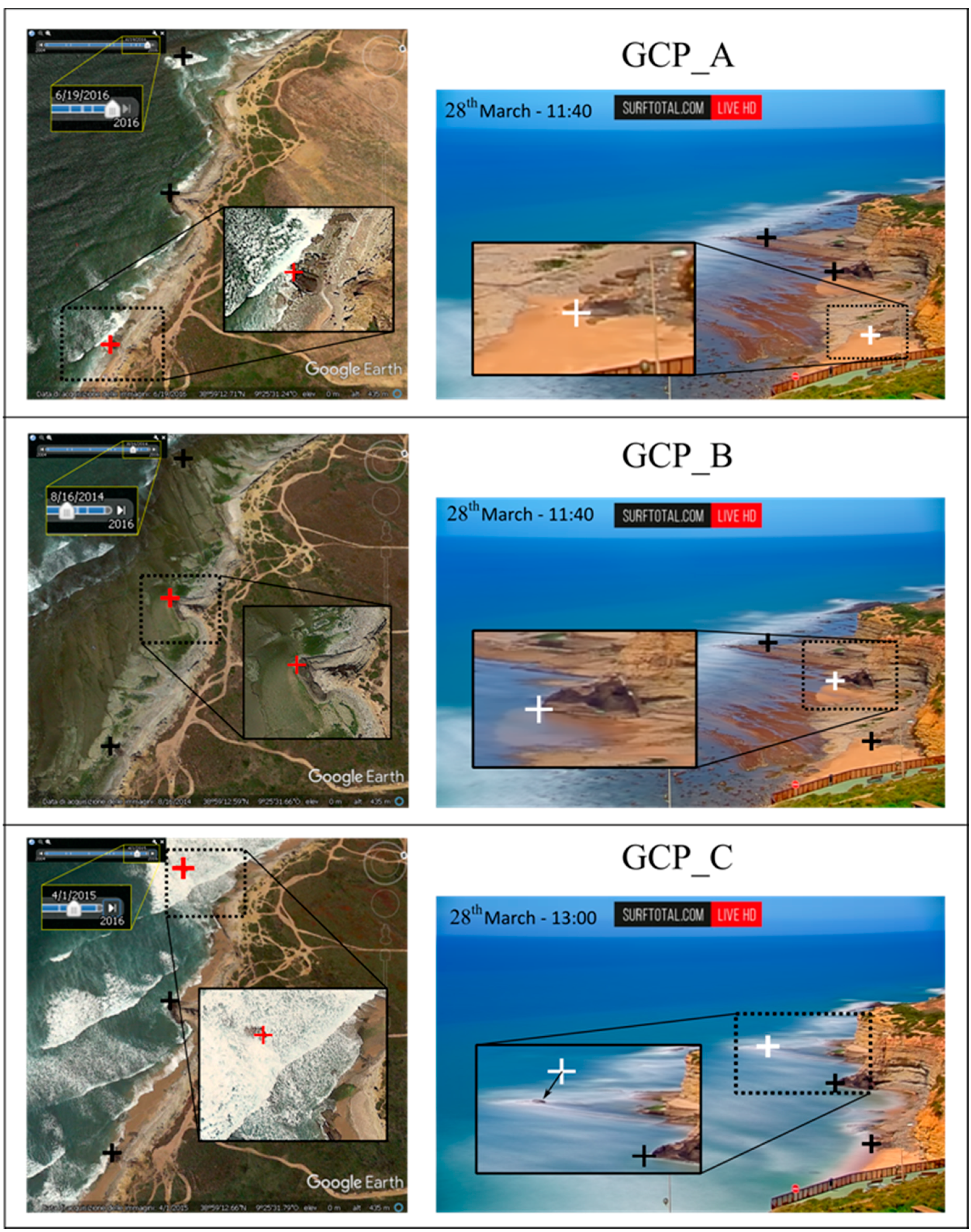
A first analysis consisted in finding distinct features which could be used as GCPs (Figure 4), visible both on the available Google Earth images and on the surfcam image. A first feasible element was identified in a big dark rock on the shore, at the foot of the cliff (GCP_A). This point was also well visible at the same position in Google Earth images from 2016, 2015 and 2014. The second point (GCP_B) was found on the spike of the headland which limited the Ribeira d’Ilhas beach northward. The Google Earth image from 2014, which was acquired during low tide conditions, allowed the selection of the right position in accordance with surfcam image, as the headland was not covered by water. The third point (GCP_C) was identified on the rock that was still emerged in the surfcam image during high tide, when water level covered the whole rocky platform. The specific tidal condition coincided on the 2015 image of Google Earth, where the piece of the rock was also visible in the same position.
Since the elevation data supplied by Google Earth still does not have the required accuracy [79,80,81,82,83], the elevation of the GCPs was estimated using a procedure that took advantages of Timex images properties. As seen in Section 1.2, the high-frequency swash oscillation on the beach is average out on Timex, therefore these images have been extensively used to identify the shoreline as land–water interface. Here, firstly, a specific algorithm identified the shoreline contour (Figure 5) as the cross-shore location of maximum gradient in the ratio of the red to green color band on the oblique 10-min RGB Timex images (e.g., [84,85]), limiting the shoreline detection to the sector in which GCP_A, GCP_B and GCP_C were located.
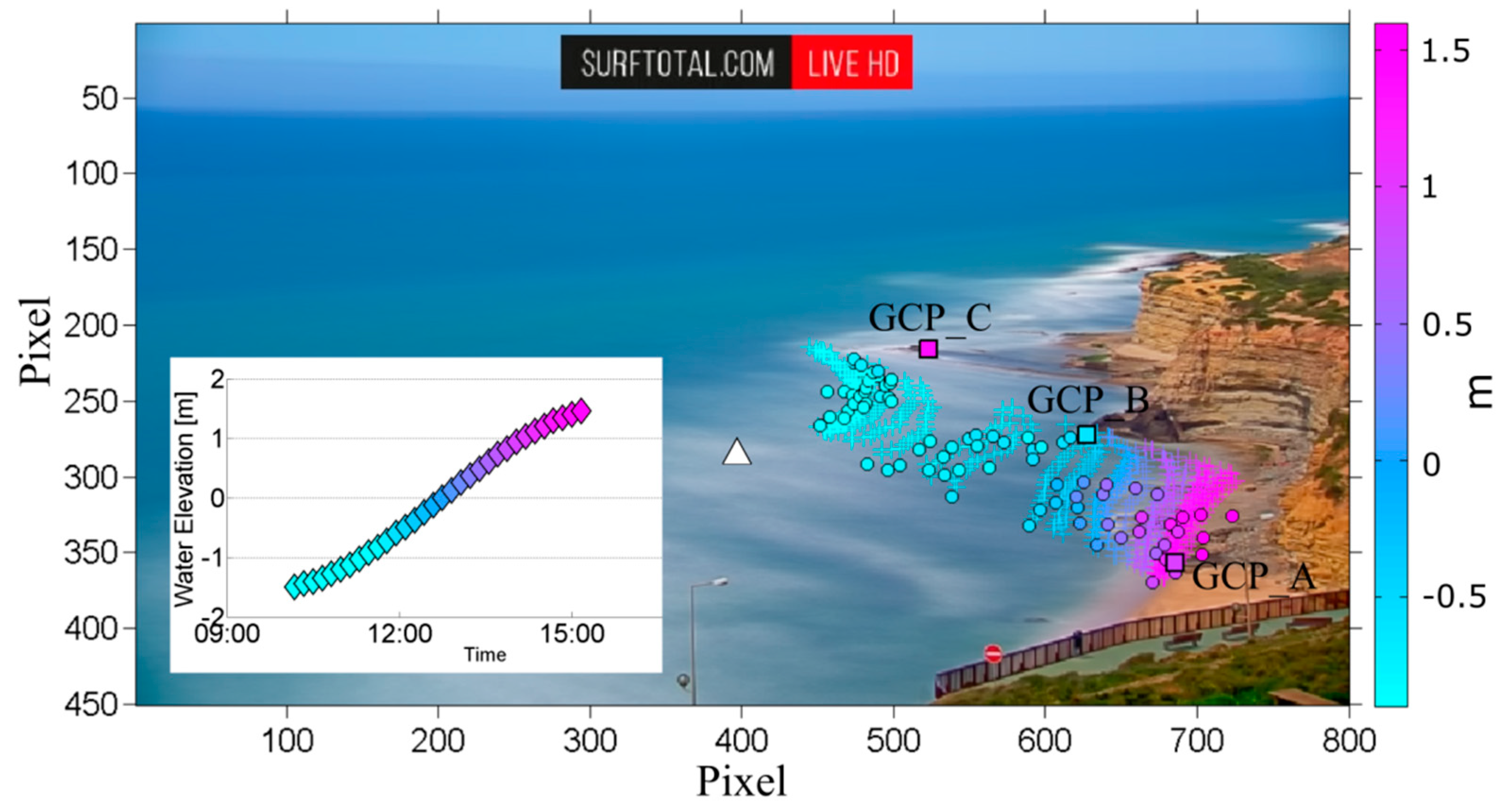
Secondly, each shoreline elevation was assumed to be equal to the tidal level measured from the online-retrieved TG dataset (Section 3.2) at the corresponding Timex production time. Figure 5 shows the 32 shoreline contours detected over the tidal cycle, and compares the GCPs elevation surveyed from RTK-GPS instrumentation to give also a first visual perception of the goodness of fit.
The three identified GCPs elevation was assumed to be equal to the elevation of the shoreline elevation intersecting the points. GCP_A was intercepted by the shoreline that was marked on the Timex image produced at 14:00, corresponding to water level η = −0.95. GCP_B by the shoreline at η = −0.60 at 12:00. GCP_C elevation was, instead, associated to the time in which the rock was fully covered, corresponding at tidal level η = 1.45 at 15:00. The accuracy of this procedure was evaluated comparing the three GCPs elevation with the closest-located terrain points elevation surveyed by RTK-GPS instrumentation. All GCPs coordinates (Table 1) were converted from WGS84 to the local projected coordinate system (ETRS 86—Portugal TM06) through freely accessible transformation codes available online [86]. Hereinafter, we refer to these remotely retrieved GCPs as “Method 2”.
3.5. Method 2—Camera Position from Web Tool
Google Earth fully integrates Google Street View, which is a tool that displays 360° panoramic street-level photos taken by cameras mounted on automobiles (e.g., [87]). Images can be viewed at different scales, from many angles, and are navigable by arrow icons imposed on them.
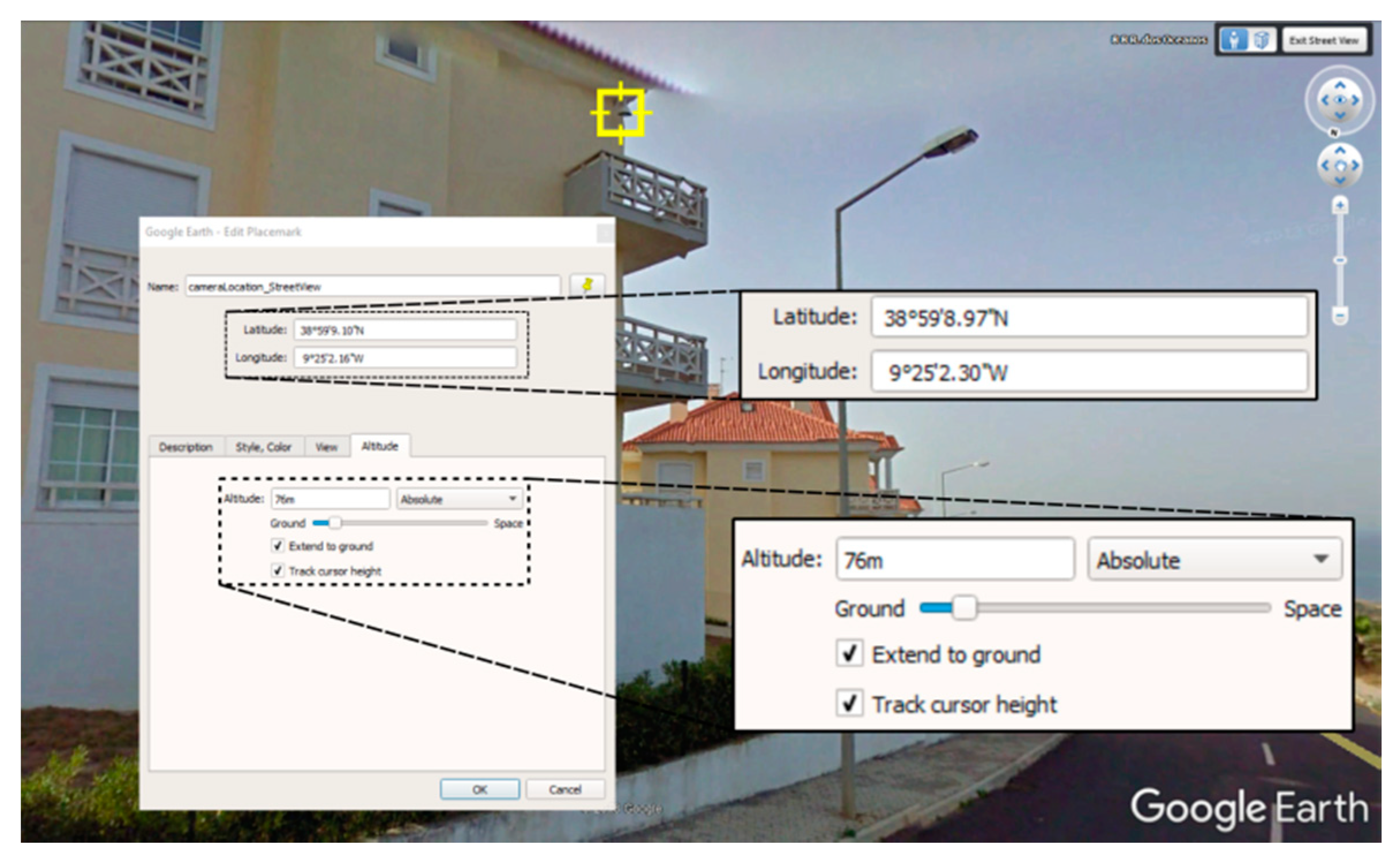
In the case study, the surfcam was installed at the last floor of a house located on the hill dominating the littoral. From the analysis of Google Street View (Figure 6), camera position was found at location 38°59′09.00″N, 9°25′02.33″W. With the option “terrain” activated on Google Earth software, it was also possible to get the estimated elevation of the camera in 76 m.
3.6. Practical Implementation of C-Pro
This sub-section describes the methodological steps undertook by C-Pro tool to produce rectified planar images through the use of the GCPs collected from the two Methods presented in Section 3.3 and Section 3.4. The procedures differ in the number of available GCPs and in the amount of known and unknown parameters considered to compute an iterative weighted least squares fitting over the linearized collinearity equations. For a detailed description of C-Pro computational steps, please refer to Sánchez-García et al. [76].
The procedures are numbered following the considered GCPs for the computation, namely Procedure 1 and Procedure 2, recalling the methods that were used to retrieve the points (Section 3.3 and Section 3.4).
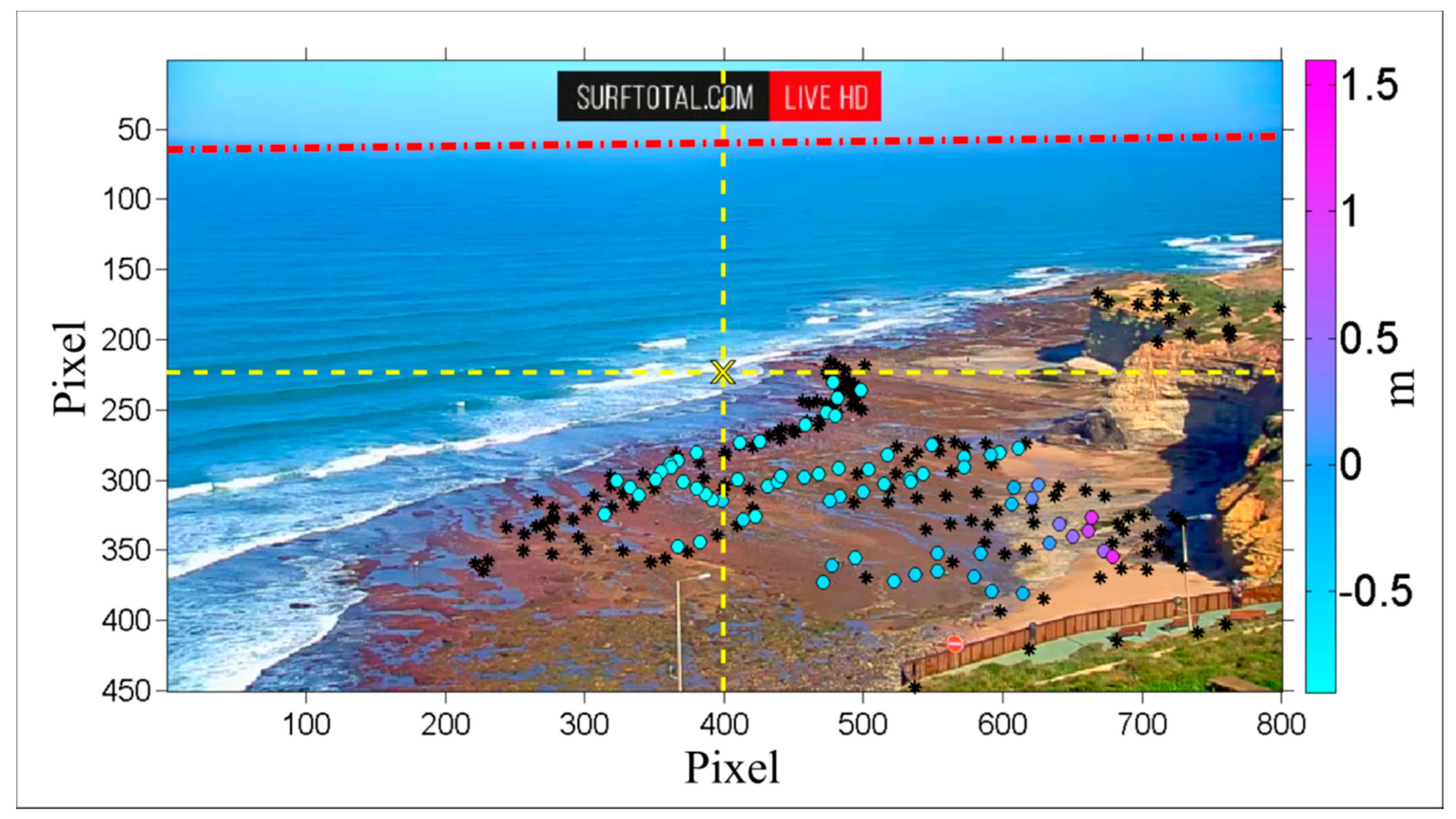
3.6.1. Procedure 1
Among the 206 points collected in the field by the conventional RTK-GPS survey (Method 1), 72 were chosen as GCPs, heterogeneously distributed on the rocky platform (Figure 7). As the number of available GCPs was more than six, C-Pro tool computed firstly the 11 DLT coefficients that express the relationships between terrain coordinates and image space. This initial step led to first approximated values of focal length f and camera location (XC, YC, ZC). The first estimation of the three-angle describing camera orientation (α, τ, θ) came instead from the horizon constraint detected on surfcam image (Figure 7). In the second computational step, the approximated values of f and EOPs were used as input data to complete the collinearity least squares fitting, whose iterative process finished when each of the correction values for the seven parameters became negligible. Although the high number of GCPs promoted an over-determined system to solve the geometry, the two extra horizon equations were included in the iterative process to improve the camera repositioning result. The final step consisted in using the optimized IOPs and EOPs to generate a georectified planar Timex image. The image was projected on a specific plane through an inverse mapping technique and applying the nearest neighbor interpolation method. The Z elevation value for the projected plane was taken equal to the tidal level at the correspondent image time.
Among the 206 terrain points, the remaining 134 terrain points—not chosen as GCPs—were used as checkpoints (Figure 7) to assess the goodness of the photogrammetric solution and the positional accuracy of the rectified image generated by C-Pro. The horizontal projection error for the 134 checkpoints was found firstly projecting each point on its associated altimetric Z coordinate (measured by RTK-GPS), finally computing the Euclidean distance between its projected coordinates (X, Y) and its real-world coordinates measured in the field. The camera location computed by C-Pro was compared to the one retrieved from Google Street View (Section 3.5).
3.6.2. Procedure 2
A second example of C-Pro application (Procedure 2) considered the three GCPs remotely-retrieved in Method 2. Here, two sub-examples of C-Pro computations were made.
In the first sub-example (Procedure 2a), C-Pro used the camera coordinates obtained from Google Street View (Section 3.5) as initial camera position. A first value of the focal length f = 1500 pixels was randomly guessed, while the initial camera orientation (α, τ, θ) was obtained from the horizon line detected on image, as in Procedure 1. Because of the limited number of available GCPs, the DLT method could not be used; therefore, the computation started directly with the iterative least squares fitting over the linearized collinearity equations. Since the six collinearity equations (two for each GCP) were not enough to solve the iterative process and to optimize the seven guessed parameters (f, XC, YC, ZC, α, τ, θ), the two horizon equations were added to solve the system. Adding these two equations ensured a solution of the system with one degree of freedom (DoF), given that DoFs are calculated as the difference between the number of equations and unknown parameters to estimate.
The second sub-example (Procedure 2b) aimed to investigate if using the remotely-retrieved camera position (Section 3.5) could assess a better solution. A first preliminary computation (Procedure 2b’) set steady and locked the remotely-retrieved camera location, in order to find the remaining free parameters (f, α, τ, θ) with four DoFs. As it is assumed that remotely retrieved camera 3D coordinates are a rough approximation, a second iteration (Procedure 2b) was set to attempt an optimization and to minimize the misfit. Taken the preliminary results as input values, a second adjustment (Procedure 2b) released the camera position and fixed the focal length f retrieved from Procedure 2b’ in order to solve the remaining six external parameters (XC, YC, ZC, α, τ, θ) with two DoFs.
A rectified image was generated from both Procedure 2a and Procedure 2b, following the same methodology adopted in Procedure 1. The positional accuracy of the rectified images was evaluated calculating the projection error for the same 134 checkpoints considered in Procedure 1, and therefore a direct comparison among the Procedures could be made. Table 2 resumes the details of each computational procedure, indicating which parameters were free to vary or have being considered fixed through the iterative process.
4. Results
4.1. Surfcam Case Study
Figure 8 shows the relation between the shoreline elevations, assumed to be at water level, and the RTK-GPS surveyed elevation of those points that were intercepted among the all 206 points. In total, 79 points were intercepted by the shorelines (refer to Figure 5). The fully-remote Method 2 underestimated point elevation with a median value of 0.3 m, a root mean square error (RMSE) of 0.48 m, and highest difference of 1 m. For completeness, Figure 8 also shows the relation of GCPs elevation with shoreline elevation taken at the water level measured by the deployed PT. Using values measured in the field, the points elevation would have been better estimated, since the median difference to surveyed elevations was about 0.05 m and RMSE = 0.33 m. The difference between TG and PT water level was almost constant for the whole considered period of 5 h, when PT measured a water level higher 0.15 m than TG, difference that might be related to local wave setup.
Finally, concerning the three GCPs estimated from Method 2, a direct comparison with RTK-GPS was not possible because these specific points were not collected during the field experience, as the remote method was developed successively. Nonetheless, their elevation was in agreement with closest surveyed GCPs available from the in-situ survey (Figure 8, Right), with disparities of about −0.05 m (GCP_A), +0.01 m (GCP_B) and +1 m (GCP_C).
4.2. Projection Error
Figure 9 shows the planar images produced from the three C-Pro computational procedures, along with the horizontal projection error for the 134 checkpoints. From a first visual analysis, the projection error on the rectified Timex produced from Procedure 1 was appropriately sorted over the whole area, with all the points projected with a horizontal accuracy lower than 5 m. On the rectified Timex obtained from Procedure 2a, some points show higher projection error, with the highest bias for those points located on the cliff (projection error between 8 m and 15 m). Finally, Procedure 2b generated a planar Timex in which projection error looked significant for the points located close to the waterline, while misfit for the checkpoints located close to the shoreline was in line with the other Procedures. Overall, all images generated by the three procedures were in agreement with the basemap. Among all checkpoints, 119 points were located on the rocky intertidal platform, which is the target area for most hydrodynamic and morphological coastal studies (e.g., [87]).
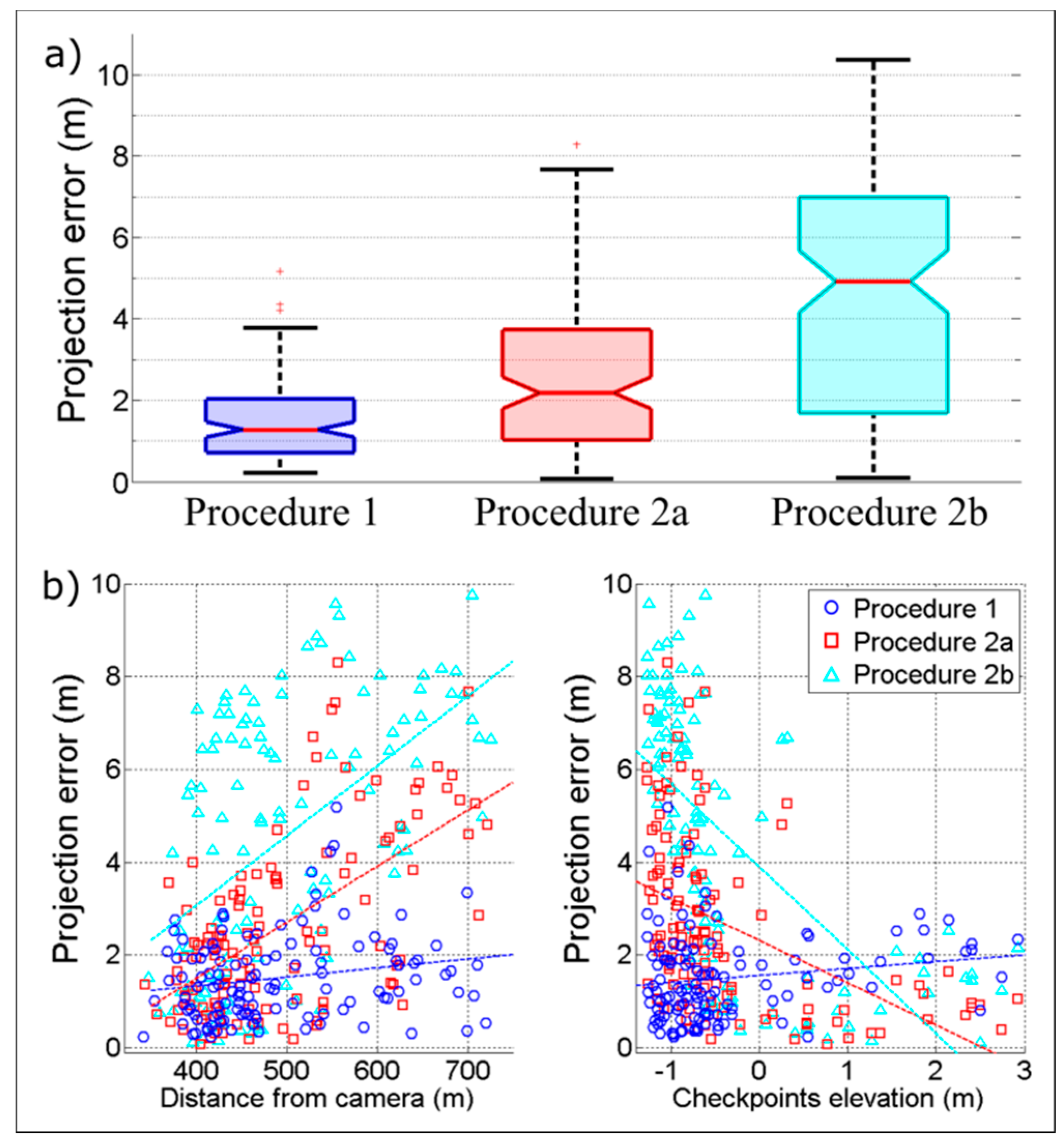
Figure 10 shows the statistical analysis of the positional accuracy depending on the projection error, limited to these 119 checkpoints, whose elevation ranged from −1.3 m and 3 m (MSL). From Procedure 1, the total median projection error was of 1.3 m, with 75% of the checkpoints position within 2 m of accuracy. Highest disparities were around 5 m, registered at some checkpoints points with −1 m elevation. The error was almost constant across the whole area, and no significant relation was found both to camera distance and to checkpoints elevation. On the contrary, results from Procedure 2a showed a stronger correlation to camera distance, as error increased as much as checkpoints were farther from the camera. Total median projection bias was of 2.2 m, with 90 points repositioned with a misfit within the 3.75 m. Finally, Procedure 2b showed the lowest projection accuracy, with a median error of 5 m and maximum error of about 10 m. As previously notable in Figure 9, projection error from Procedure 2b was strongly dependent on checkpoint location in relation both to camera position and to checkpoint elevation.
4.3. Camera Parameters
Table 3 summarizes the values of internal and external camera parameters obtained from the different Procedures. Results from Procedure 1 and Procedure 2a were similar, although the different number and sources of GCPs used for the procedures. Camera position was found around 9–10 m far from the remotely-derived camera location, with major displacement along longitude (easting), at an elevation of about 80 m.
On the other hand, fixing the camera position with the remotely-derived camera coordinates and elevation in Procedure 2b resulted in a computation of a larger focal length of about 110 pixels in comparison with that obtained from Procedure 1 and Procedure 2a. The overestimation of the focal length might be the cause of the highest projection error obtained from Procedure 2b (Figure 10). In fact, a longer focal length coupled to a lower camera elevation reproduced a narrower angle of view of the scene and a higher magnification of the scene. These might be determined by the high dependence of projection error on checkpoint elevation and location, since points were “virtually” seen with a lower angle.
5. Discussion
The rectified surfcam image from Procedure 1 represents a quite satisfactory achievement, especially if considering the initial conditions (unknown IOPs and EOPs), the low image resolution (800 × 450) and the high distance between the camera and the GCPs (between 350 and 700 m). In addition, the (low) projection error was well distributed in the nearshore area. Taking in account that a high number of GCPs (72) were used in the iterative process, projection accuracy might be even improved by resampling the GCPs for a better identification in the original images, or by choosing a different spatial configuration of the points.
The results obtained from Procedure 2a were satisfactory. C-Pro tool was able to retrieve the same focal length and camera orientation as in Procedure 1, although the computation was based on just three remotely-sensed GCPs. In this perspective, the presented methodology to derive the GCPs coordinates from Google Earth and GCPs elevation from shoreline position (Method 2) appears to be a practical and viable solution to collect the GCPs required for image rectification remotely. The relative small error and the overall accordance between remotely-derived GCPs and surveyed points (Figure 8) proved the robustness of the proposed methodology. Alternative mapping sources are numerous (e.g., ESRI ArcMap), nevertheless Google Earth is distinctive in offering the easy, fast and free access to several images taken during different sea state conditions over the years. In the case study, this specific characteristic allowed to spot specific points that were visible during certain tidal conditions. In this work, additional GCPs could also be identified on the cliff and on the terrace-parking viewpoint, both on surfcam image and satellite images. However, these points were not considered suitable for the aim of this work as the elevation of area of interest was near sea level and the elevation of those points could not be accurately estimated remotely. In fact, Google Earth elevation data should be considered carefully. For example, the elevation on Google Earth terrain map of the three GCPs (GCP_A, GPC_B and GPC_C) were 9 m, 8 m and 2 m, respectively, far from the true elevation, that was successfully deduced from Method 2. Nevertheless, the technique of deriving GCPs elevation from shoreline in Method 2 was particularly effective because of the site-specific low gradient slope (tanβ = 0.01) of the rocky platform of Ribeira d’Ilhas. Here, the meso-tidal range (~2.8 m) made moving the local shoreline on a wide cross-shore span of about 400 m over the observed time. Alternative remote-sensing sources for retrieving GCPs elevation are the aerial LiDAR (e.g., [88,89,90]), satellite altimetry data (e.g., [91]) or unmanned aerial vehicle (UAV) (e.g., [92]). However, these types of data are not always available and/or do not have the adequate resolution, and/or require intensive computational effort which would make more difficult the methodology. In addition, it should be considered that in case of study sites such as sandy shores, the intertidal area and emerged beach profile often change in shape and elevation due to the high dynamicity of sediment driven by wave forcing, so the use of synoptic data is advisable. In this perspective, future works should investigate the combined use of Google Earth, Google Street View and other optical sources to take advantages of site-specific presence of fixed elements such as coastal structures, touristic installations, urban infrastructures, along with geographical constraints, that can support the extraction of GCPs within the field of view of online streamed images. As final remark regarding Method 2, the key requirement of water level was supplied by an available dataset retrieved online (TG). In case of absence of a proper record of data, freely available tide predictors can be used (e.g., https://www.wtides.com, https://www.tide-forecast.com).
The lower accuracy achieved from Procedure 2a in respect to Procedure 1 may be due several uncertainties added during the process. A first reason might be related to the small number of GCPs used for resection, as the image area was not well covered by the points. Secondly, the procedure of marking the GCPs, both on satellite image and on surfcam frame, is subjective and prone to error. Thirdly, shoreline elevation to estimate GCPs height was simply considered equal to tidal level, although previous works proved that swash excursion and wave set up contributions should be taken in account for assessing shoreline elevation (e.g., [4,12]). This explains the closer relation found between GCPs elevation and water level measured by the PT in the nearshore (Figure 8). Finally, Google Earth image horizontal resolution also has impact on the final result, as it can change in space and time (e.g., [93,94]).
Computed camera positional error in relation to the remotely-derived surfcam location looked to be not significant in the rectification process, as C-Pro can compensate such error with a different estimation of the three angles (α, τ, θ) which describe the camera orientation. On the contrary, C-Pro results were considerably sensitive to camera elevation, since fixing camera elevation found from Google Street View in Procedure 2b led to an overestimation of the focal length and determined larger projection errors. The Procedure 2b test finally suggests that future works should not consider fix the remotely-retrieved camera position through the iterative process, since C-Pro performs better when all parameters are set free to be adjusted.
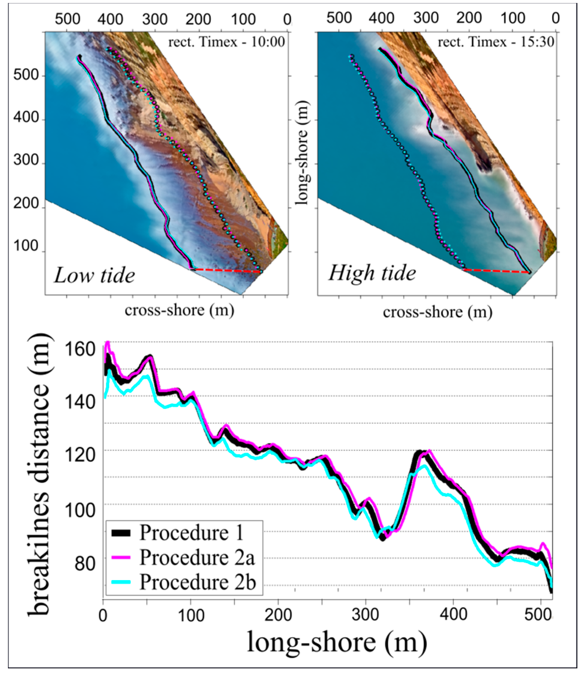
Common to all C-Pro procedures was the fact that lens-inducted distortions have been considered negligible. Future works should carefully analyze image properties and in case taking in account the image curvature, as one preliminary C-Pro computational step can be added to compute the distortion coefficients and correct the skewness of the image. In general, it should be stressed out that most video monitoring applications in coastal studies do not rely on absolute location but, instead, on relative positioning. For instance, morphological analysis (see Section 1.2 for a detailed video monitoring applications description) of the shoreline change, offshore bar migration, along with the estimation of hydrodynamics such as wave height, need a planar image to simply associate pixel features to geometry measurements; therefore, the images should be appropriately corrected from perspective distortions and accurately rectified, but do not require a precise absolute positioning. For instance, Figure 11 shows the comparison among the water breaklines detected on the planar images generated from each procedure, during low tide and high tide. Breaklines were found sampling a series of cross-shore pixel transects and identified at the pixel with highest intensity (e.g., [17,18]). Comparing the position among breaklines found on Timex rectified by Procedure 1 and the other two examples (Procedure 2a and Procedure 2b), median differences were in the range of 1–2 m for both low and high tide. From the analysis of the distances between breaklines obtained on images with same procedure, it can be seen that Procedure 1 and Procedure 2a were in agreement (about 1 m of difference on median value), while the distance was slightly shorter in Procedure 2b. For this last example, median disparity with the other two procedures was about 3 m, with a maximum disparity of 11 m. These values represent around the 6% of the total distance calculated between breaklines, and thus can be considered not significant for a quantitative analysis.
Overall, both results from Procedure 1 and Procedure 2a were in line with other works that used a standard georectification technique for coastal imagery analysis (e.g., [5,6,7,8]), and proved the suitability of the methodological steps presented in this work.
As a final remark, the C-Pro tool can also be easily implemented in the existing image rectification softwares. For instance, the parameters assessed by C-Pro in Procedure 1 were implemented in an automatic version of COSMOS software [6] to rectify the whole image sequence obtained at Ribeira d’Ilhas, which was used for the development of new methodologies to estimate nearshore hydrodynamics and morphology [95]. Nonetheless, C-Pro is an independent coastal projector monitoring system that is freely available upon request to the authors.
6. Conclusions
This communication presented operational applications of C-Pro projection tool to obtain rectified planar images from an online streaming camera. Two examples to retrieve GCPs were presented. A first method used the in-situ standard RTK-GPS instrumentation for the collection of points, while a second novel methodology derived GCP location and elevation coupling Google Earth historical images to shoreline detection on video imagery. C-Pro has been shown to work efficiently with both in-situ and remotely-derived GCPs, estimating the seven unknown parameters of the camera to generate accurate georectified images. The median horizontal projection errors obtained by Procedure 1 and Procedure 2a were acceptable, being of 1.3 m and 2.2 m, respectively, whereas Procedure 2b was less accurate with 5 m of median positional misfit. The presented procedures promote the use of online streaming images for the application of a coastal video monitoring technique, avoiding the installation of new monitoring systems. The methodologies give the opportunity to turn surfcam infrastructure into a fully remote shore-based observational system in order to apply the video-based scientific techniques for improving knowledge of coastal processes.
Author Contributions
Conceptualization, U.A.; Methodology, U.A. and E.S.-G.; Formal Analysis, U.A. and E.S.-G.; Investigation, U.A. and E.S.-G.; Writing-Original Draft Preparation, U.A.; Writing-Review & Editing, U.A., E.S.-G. and R.T.; Supervision, R.T.; Project Administration, R.T.; Funding Acquisition, R.T.
Funding
Umberto Andriolo was supported by the EARTHSYSTEM Doctorate Programme (SFRH/BD/52558/2014). This study is part of the PhD dissertation of E. Sánchez-García, which was supported by a grant from the Spanish Ministry of Education, Culture and Sports (I + D + i 2013–2016) and supported by the Spanish Ministry of Economy, Industry and Competitiveness under project CGL2015-69906-R. Publication supported by FCT- project UID/GEO/50019/2013 - Instituto Dom Luiz.
Acknowledgments
The authors of this work are also grateful to A. Fortunato, C. Lira and D. Mendes for their support during field work.
Conflicts of Interest
The authors declare no conflict of interest.
References
- Short, A.D.; Trembanis, A.C. Decadal Scale Patterns in Beach Oscillation and Rotation Narrabeen Beach, Australia—Time Series, PCA and Wavelet Analysis. J. Coast. Res. 2004, 202, 523–532. [Google Scholar] [CrossRef]
- Mason, D.C.; Gurney, C.; Kennett, M. Beach topography mapping—A comparison of techniques. J. Coast. Conserv. 2000, 6, 113–124. [Google Scholar] [CrossRef]
- Holman, R.A.; Stanley, J. The history and technical capabilities of Argus. Coast. Eng. 2007, 54, 477–491. [Google Scholar] [CrossRef]
- Aarninkhof, S.G.J.; Turner, I.L.; Dronkers, T.D.T.; Caljouw, M.; Nipius, L. A video-based technique for mapping intertidal beach bathymetry. Coast. Eng. 2003, 49, 275–289. [Google Scholar] [CrossRef]
- Nieto, M.A.; Garau, B.; Balle, S.; Simarro, G.; Zarruk, G.A.; Ortiz, A.; Orfila, A. An open source, low cost video-based coastal monitoring system. Earth Surf. Process. Landf. 2010, 35, 1712–1719. [Google Scholar] [CrossRef] [Green Version]
- Taborda, R.; Silva, A. COSMOS: A lightweight coastal video monitoring system. Comput. Geosci. 2012, 49, 248–255. [Google Scholar] [CrossRef]
- Brignone, M.; Schiaffino, C.F.; Isla, F.I.; Ferrari, M. A system for beach video-monitoring: Beachkeeper plus. Comput. Geosci. 2012, 49, 53–61. [Google Scholar] [CrossRef]
- Simarro, G.; Ribas, F.; Álvarez, A.; Guillén, J.; Chic, Ò.; Orfila, A. ULISES: An Open Source Code for Extrinsic Calibrations and Planview Generations in Coastal Video Monitoring Systems. J. Coast. Res. 2017, 335, 1217–1227. [Google Scholar] [CrossRef]
- Vousdoukas, M.I.; Ferreira, P.M.; Almeida, L.P.; Dodet, G.; Psaros, F.; Andriolo, U.; Taborda, R.; Silva, A.N.; Ruano, A.; Ferreira, Ó.M. Performance of intertidal topography video monitoring of a meso-tidal reflective beach in South Portugal. Ocean Dyn. 2011, 61, 1521–1540. [Google Scholar] [CrossRef]
- Hartley, R.; Zisserman, A. Multiple View Geometry in Computer Vision, 2nd ed.; Cambridge University Press: Cambridge, UK, 2003. [Google Scholar]
- Camera Calibration Toolbox for Matlab. Available online: http://www.vision.caltech.edu/bouguetj/calib_doc/ (accessed on 20 November 2018).
- Andriolo, U.; Almeida, L.P.; Almar, R. Coupling terrestrial LiDAR and video imagery to perform 3D intertidal beach topography. Coast. Eng. 2018, 140, 232–239. [Google Scholar] [CrossRef]
- Holland, K.T.; Holman, R.A.; Lippmann, T.C. Practical use of video imagery in nearshore oceanographic field studies’. IEEE J. Ocean Eng. 1997, 22, 81–92. [Google Scholar] [CrossRef]
- Bechle, A.J.; Wu, C.H.; Liu, W.; Kimura, N. Development and Application of an Automated River-Estuary Discharge Imaging System. J. Hydraul. Eng. 2012, 138, 327–339. [Google Scholar] [CrossRef]
- Harley, M.D.; Andriolo, U.; Armaroli, C.; Ciavola, P. Shoreline rotation and response to nourishment of a gravel embayed beach using a low-cost video monitoring technique: San Michele-Sassi Neri, Central Italy. J. Coast. Conserv. 2013, 18, 551–565. [Google Scholar] [CrossRef]
- Lippmann, T.C.; Holman, R.A. Quantification of sand bar morphology: A video technique based on wave dissipation. J. Geophys. Res. 1989, 94, 995–1011. [Google Scholar] [CrossRef]
- Armaroli, C.; Ciavola, P. Dynamics of a nearshore bar system in the northern Adriatic: A video-based morphological classification. Geomorphology 2011, 126, 201–216. [Google Scholar] [CrossRef]
- Balouin, Y.; Tesson, J.; Gervais, M. Cuspate shoreline relationship with nearshore bar dynamics during storm events—Field observations at Sete beach, France. J. Coast. Res. 2013, 65, 440–445. [Google Scholar] [CrossRef]
- Angnuureng, D.B.; Almar, R.; Senechal, N.; Castelle, B.; Addo, K.A.; Marieu, V.; Ranasinghe, R. Shoreline resilience to individual storms and storm clusters on a meso-macrotidal barred beach. Geomorphology 2017, 290, 265–276. [Google Scholar] [CrossRef]
- Turner, I.L.; Whyte, D.; Ruessink, B.; Ranasinghe, R. Observations of rip spacing, persistence and mobility at a long, straight coastline. Mar. Geol. 2007, 236, 209–221. [Google Scholar] [CrossRef]
- Orzech, M.D.; Thornton, E.B.; MacMahan, J.H.; O’Reilly, W.C.; Stanton, T.P. Alongshore rip channel migration and sediment transport. Mar. Geol. 2010, 271, 278–291. [Google Scholar] [CrossRef]
- Gallop, S.; Bryan, K.; Coco, G.; Stephens, S. Storm-driven changes in rip channel patterns on an embayed beach. Geomorphology 2011, 127, 179–188. [Google Scholar] [CrossRef]
- Pitman, S.; Gallop, S.L.; Haigh, I.D.; Masselink, G.; Ranasinghe, R. Wave breaking patterns control rip current flow regimes and surfzone retention. Mar. Geol. 2016, 382, 176–190. [Google Scholar] [CrossRef] [Green Version]
- Ranasinghe, R.; Symonds, G.; Black, K.; Holman, R. Morphodynamics of intermediate beaches: A video imaging and numerical modelling study. Coast. Eng. 2004, 51, 629–655. [Google Scholar] [CrossRef]
- Quartel, S.; Addink, E.; Ruessink, B. Object-oriented extraction of beach morphology from video images. Int. J. Appl. Earth Obs. Geoinf. 2006, 8, 256–269. [Google Scholar] [CrossRef]
- Ortega-Sánchez, M.; Fachin, S.; Sancho, F.; Losada, M.A. Relation between beachface morphology and wave climate at Trafalgar beach (Cádiz, Spain). Geomorphology 2008, 99, 171–185. [Google Scholar] [CrossRef]
- Price, T.; Ruessink, B. Morphodynamic zone variability on a microtidal barred beach. Mar. Geol. 2008, 251, 98–109. [Google Scholar] [CrossRef]
- Masselink, G.; Austin, M.; Scott, T.; Poate, T.; Russell, P. Role of wave forcing, storms and NAO in outer bar dynamics on a high-energy, macro-tidal beach. Geomorphology 2014, 226, 76–93. [Google Scholar] [CrossRef] [Green Version]
- Alvarez-Ellacuria, A.; Orfila, A.; Gómez-Pujol, L.; Simarro, G.; Obregon, N. Decoupling spatial and temporal patterns in short-term beach shoreline response to wave climate. Geomorphology 2011, 128, 199–208. [Google Scholar] [CrossRef] [Green Version]
- Osorio, A.; Medina, R.; Gonzalez, M. An algorithm for the measurement of shoreline and intertidal beach profiles using video imagery: PSDM. Comput. Geosci. 2012, 46, 196–207. [Google Scholar] [CrossRef]
- Valentini, N.; Saponieri, A.; Molfetta, M.G.; Damiani, L. New algorithms for shoreline monitoring from coastal video systems. Earth Sci. Inform. 2017, 10, 495–506. [Google Scholar] [CrossRef]
- Ruiz de Alegria-Arzaburu, A.; Masselink, G. Storm response and beach rotation on a gravel beach, Slapton Sands, U.K. Mar. Geol. 2010, 278, 77–99. [Google Scholar] [CrossRef]
- Blossier, B.; Bryan, K.R.; Daly, C.J.; Winter, C. Spatial and temporal scales of shoreline morphodynamics derived from video camera observations for the island of Sylt, German Wadden Sea. Geo-Mar. Lett. 2017, 37, 111. [Google Scholar] [CrossRef]
- Fairley, I.; Davidson, M.; Kingston, K.; Dolphin, T.; Phillips, R. Empirical orthogonal function analysis of shoreline changes behind two different designs of detached breakwaters. Coast. Eng. 2009, 56, 1097–1108. [Google Scholar] [CrossRef]
- Simarro, G.; Bryan, K.R.; Guedes, R.M.; Sancho, A.; Guillen, J.; Coco, G. On the use of variance images for runup and shoreline detection. Coast. Eng. 2015, 99, 136–147. [Google Scholar] [CrossRef]
- Rigos, A.; Tsekouras, G.E.; Vousdoukas, M.I.; Chatzipavlis, A.; Velegrakis, A.F. A Chebyshev polynomial radial basis function neural network for automated shoreline extraction from coastal imagery. Integr. Comput-Aid. Eng. 2016, 23, 141–160. [Google Scholar] [CrossRef]
- Stockdon, H.F.; Holman, R.A.; Howd, P.A.; Sallenger, A.H. Empirical parameterization of setup, swash, and runup. Coast. Eng. 2006, 53, 573–588. [Google Scholar] [CrossRef]
- Almar, R.; Cienfuegos, R.; Catalán, P.A.; Birrien, F.; Castelle, B.; Michallet, H. Nearshore bathymetric inversion from video using a fully non-linear Boussinesq wave model. J. Coast. Res. 2011, 64, 3–7. [Google Scholar]
- Aagaard, T.; Holm, D. Digitization of wave runup using video records. J. Coast. Res. 1989, 5, 547–551. [Google Scholar]
- Holland, K.T.; Holman, R.A. The statistical distribution of swash maxima on natural beaches. J. Geophys. Res. 1993, 98, 10271–10278. [Google Scholar] [CrossRef]
- Birkemeier, W.A.; Donohue, C.; Long, C.E.; Hathaway, K.K.; Baron, C.F. The 1990 DELILAH Nearshore Experiment: Summary Report; Technical Report CHL-97-24; U.S. Army Corps of Engineers, Waterways Experiment Station: Vicksburg, MS, USA, 1997. [Google Scholar]
- Bailey, D.G.; Shand, R.D. Determining Wave Run-up using Automated Video Analysis. In Proceedings of the 2nd NZ Conference on Image and Vision Computing, Palmerston North, New Zealand, August 1994. [Google Scholar]
- Holland, K.T.; Raubenheimer, B.; Guza, R.T.; Holman, R.A. Runup kinematics on a natural beach. J. Geophys. Res. 1995, 100, 4985. [Google Scholar] [CrossRef]
- Ruggiero, P.; Holman, R.A.; Beach, R.A. Wave run-up on a high energy dissipative beach. J. Geophys. Res. 2004, 109. [Google Scholar] [CrossRef]
- Vousdoukas, M.I.; Velegrakis, A.F.; Dimou, K.; Zervakis, V.; Conley, D.C. Wave run-up observations in microtidal, sediment-starved pocket beaches of the Eastern Mediterranean. J. Mar. Syst. 2009, 78, S37–S47. [Google Scholar] [CrossRef]
- Guedes, R.M.C.; Bryan, K.R.; Coco, G.; Holman, R.A. The effects of tides on swash statistics on an intermediate beach. J. Geophys. Res. Oceans 2011, 116, 1–13. [Google Scholar] [CrossRef]
- Power, H.E.; Holman, R.A.; Baldock, T.E. Swash zone boundary conditions derived from optical remote sensing of swash zone flow patterns. J. Geophys. Res. Oceans 2011, 116. [Google Scholar] [CrossRef] [Green Version]
- Senechal, N.; Coco, G.; Bryan, K.R.; Holman, R.A. Wave runup during extreme storm conditions. J. Geophys. Res. Oceans 2011, 116. [Google Scholar] [CrossRef] [Green Version]
- Brinkkemper, J.A.; Lanckriet, T.; Grasso, F.; Puleo, J.A.; Ruessink, B.G. Observations of turbulence within the surf and swash zone of a field-scale sandy laboratory beach. Coast. Eng. 2014, 113, 62–72. [Google Scholar] [CrossRef]
- Stockdon, H.F.; Thompson, D.M.; Plant, N.G.; Long, J.W. Evaluation of wave runup predictions from numerical and parametric models. Coast. Eng. 2014, 92, 1–11. [Google Scholar] [CrossRef]
- Vousdoukas, M.; Kirupakaramoorthy, T.; Oumeraci, H.; De la Torre, M.; Wübbold, F.; Wagner, B.; Schimmels, S. The role of combined laser scanning and video techniques in monitoring wave-by-wave swash zone processes. Coast. Eng. 2014, 83, 150–165. [Google Scholar] [CrossRef]
- Blenkinsopp, C.E.; Matias, A.; Howe, D.; Castelle, B.; Marieu, V.; Turner, I.L. Wave runup and overwash on a prototype-scale sand barrier. Coast. Eng. 2016, 113, 88–103. [Google Scholar] [CrossRef] [Green Version]
- Almar, R.; Blenkinsopp, C.; Almeida, L.P.; Cienfuegos, R.; Catalán, P.A. Wave runup video motion detection using the Radon Transform. Coast. Eng. 2017, 130, 46–51. [Google Scholar] [CrossRef]
- Vousdoukas, M.I.; Wziatek, D.; Almeida, L.P. Coastal vulnerability assessment based on video wave run-up observations at a mesotidal, steep-sloped beach. Ocean Dynam. 2012, 62, 123–137. [Google Scholar] [CrossRef]
- Poate, T.G.; McCall, R.T.; Masselink, G. A new parameterisation for runup on gravel beaches. Coast. Eng. 2016, 117, 176–190. [Google Scholar] [CrossRef] [Green Version]
- Atkinson, A.L.; Power, H.E.; Moura, T.; Hammond, T.; Callaghan, D.P.; Baldock, T.E. Assessment of runup predictions by empirical models on non-truncated beaches on the south-east Australian coast. Coast. Eng. 2017, 119, 15–31. [Google Scholar] [CrossRef]
- Lippmann, T.C.; Holman, R.A. The spatial and temporal variability of sand bar morphology. J. Geophys. Res. 1990, 95, 11575–11590. [Google Scholar] [CrossRef]
- Almar, R. Morphodynamique Littorale Haute Fréquence Par Imagerie Vidéo. Ph.D. Thesis, University of Bordeaux, Bordeaux, France, 2009. [Google Scholar]
- Zikra, M.; Hashimoto, N.; Yamashiro, M.; Yokota, M.; Suzuki, K. Analysis of Directional Wave Spectra in Shallow Water Areas Using Video Image Data. Coast. Eng. J. 2012, 54. [Google Scholar] [CrossRef]
- Almar, R.; Bonneton, P.; Senechal, N.; Roelvink, D. Wave celerity from video imaging: A new method. In Proceedings of the 31st International Conference Coastal Engineering, Hamburg, Germany, 31 August–5 September 2008. [Google Scholar]
- Tissier, M.; Bonneton, P.; Almar, R.; Castelle, B.; Bonneton, N.; Nahon, A. Field measurements and non-linear prediction of wave celerity in the surf zone. Eur. J. Mech. B Fluids 2011, 30, 635–641. [Google Scholar] [CrossRef]
- Almar, R.; Michallet, H.; Cienfuegos, R.; Bonneton, P.; Tissier, M.; Ruessink, G. On the use of the Radon Transform in studying nearshore wave dynamics. Coast. Eng. 2014. [Google Scholar] [CrossRef]
- Postacchini, M.; Brocchini, M. A wave-by-wave analysis for the evaluation of the breaking-wave celerity. Appl. Ocean Res. 2014, 46, 15–27. [Google Scholar] [CrossRef]
- Stockdon, H.F.; Holman, R.A. Estimation of wave phase speed and nearshore bathymetry from video imagery. J. Geophys. Res. 2000, 15, 15–22. [Google Scholar] [CrossRef]
- Yoo, J. Nonlinear Bathymetry Inversion Based on Wave Property Estimation from Nearshore Video Imagery. Ph.D. Thesis, Georgia Institute of Technology, Atlanta, GA, USA, 2007. [Google Scholar]
- Holman, R.; Plant, N.; Holland, T. CBathy: A robust algorithm for estimating nearshore bathymetry. J. Geophys. Res. Oceans 2013, 118, 2595–2609. [Google Scholar] [CrossRef]
- Gal, Y.; Browne, M.; Lane, C. Automatic estimation of nearshore wave height from video timestacks. In Proceedings of the 2011 International Conference on Digital Image Computing: Techniques and Applications (DICTA), Noosa, Australia, 6–8 December 2011. [Google Scholar] [CrossRef]
- Almar, R.; Cienfuegos, R.; Catalán, P.A.; Michallet, H.; Castelle, B.; Bonneton, P.; Marieu, V. A new breaking wave height direct estimator from video imagery. Coast. Eng. 2012, 61, 42–48. [Google Scholar] [CrossRef]
- Gal, Y.; Browne, M.; Lane, C. Long-term automated monitoring of nearshore wave height from digital video. IEEE Trans. Geosci. Remote Sens. 2014, 52, 3412–3420. [Google Scholar] [CrossRef]
- Robertson, B.; Gharabaghi, B.; Hall, K. Prediction of Incipient Breaking Wave-Heights Using Artificial Neural Networks and Empirical Relationships. Coast. Eng. J. 2015, 57. [Google Scholar] [CrossRef]
- Matias, A.; Carrasco, A.R.; Loureiro, C.; Andriolo, U.; Masselink, G.; Guerreiro, M.; Pacheco, A.; McCall, R.; Ferreira, O.; Plomaritis, T.A. Measuring and modelling overwash hydrodynamics on a barrier island. In Proceedings of the Coastal Dynamics, ASCE, Helsingor, Denmark, 12–16 June 2017. [Google Scholar]
- Chickadel, C.C. Remote Measurements of Waves and Currents over Complex Bathymetry. Ph.D Thesis, College of Oceanic and Atmospheric Sciences, Oregon State University, Corvallis, OR, USA, 2007. [Google Scholar]
- Mole, M.A.; Mortlock, T.R.C.; Turner, I.L.; Goodwin, I.D.; Splinter, K.D.; Short, A.D. Capitalizing on the surfcam phenomenon: A pilot study in regional—Scale shoreline and inshore wave monitoring utilizing existing camera infrastructure. J. Coast. Res. 2013, 65. [Google Scholar] [CrossRef]
- Bracs, M.A.; Turner, I.L.; Splinter, K.D.; Short, A.D.; Lane, C.; Davidson, M.A.; Goodwin, I.D.; Pritchard, T.; Cameron, D. Evaluation of Opportunistic Shoreline Monitoring Capability Utilizing Existing “Surfcam” Infrastructure. J. Coast. Res. 2016, 319, 542–554. [Google Scholar] [CrossRef]
- Shand, T.D.; Bailey, D.G.; Shand, R.D. Automated Detection of Breaking Wave Height Using an Optical Technique. J. Coast. Res. 2012, 282, 671–682. [Google Scholar] [CrossRef]
- Sánchez-García, E.; Balaguer-Beser, A.; Pardo-Pascual, J.E. C-Pro: A coastal projector monitoring system using terrestrial photogrammetry with a geometric horizon constraint. ISPRS J. Photogramm. Remote Sens. 2017, 128, 255–273. [Google Scholar] [CrossRef]
- DGT. Available online: ftp://ftp.dgterritorio.pt/Maregrafos/Cascais (accessed on 20 November 2007).
- Google Earth. Available online: http://www.google.com/earth/download/ge (accessed on 20 November 2007).
- Wei, H.; Luan, X.; Li, H.; Jia, J.; Chen, Z.; Han, L. Elevation data fitting and precision analysis of Google Earth in road survey. In Proceedings of the AIP Conference Proceedings, Thessaloniki, Greece, 14–18 March 2018. [Google Scholar] [CrossRef]
- Wang, Y.; Zou, Y.; Henrickson, K.; Wang, Y.; Tang, J.; Park, B. Google Earth elevation data extraction and accuracy assessment for transportation applications. PLoS ONE 2017, 12. [Google Scholar] [CrossRef]
- El-Ashmawy, K.L. Investigation of the Accuracy of Google Earth Elevation Data. Artif. Satell. 2016, 51, 89–97. [Google Scholar] [CrossRef] [Green Version]
- Rusli, N.; Majid, M.R.; Din, A.H. Google Earth’s derived digital elevation model: A comparative assessment with Aster and SRTM data. In Proceedings of the IOP Conference Series: Earth and Environmental Science, Kuching, Malaysia, 26–29 August 2013. [Google Scholar] [CrossRef]
- Rusli, N.; Pa’suya, M.F.; Talib, N. A comparative accuracy of Google Earth height with MyGeoid, EGM96 and MSL. In Proceedings of the IOP Conference Series: Earth and Environmental Science, Kuala Lumpur, Malaysia, 13–14 April 2016. [Google Scholar] [CrossRef]
- Smith, R.K.; Bryan, K.R. Monitoring beach face volume with a combination of intermittent profiling and video imagery. J. Coast. Res. 2007, 23, 892–898. [Google Scholar] [CrossRef]
- Almar, R.; Ranasinghe, R.; Sénéchal, N.; Bonneton, P.; Roelvink, D.; Bryan, K.R.; Parisot, J. Video-Based detection of shorelines at complex meso–macro tidal beaches. J. Coast. Res. 2012, 284, 1040–1048. [Google Scholar] [CrossRef]
- Coordinates Transformation. Available online: https://epsg.io/ (accessed on 20 November 2007).
- Anguelov, D.; Dulong, C.; Filip, D.; Frueh, C.; Lafon, S.; Lyon, R.; Weaver, J. Google Street View: Capturing the World at Street Level. Computer 2010, 43, 32–38. [Google Scholar] [CrossRef]
- Wehr, A.; Lohr, U. Airborne laser scanning—An introduction and overview. ISPRS J. Photogramm. Remote Sens. 1999, 54, 68–82. [Google Scholar] [CrossRef]
- Vignudelli, S.A.; Kostianoy, P.; Cipollini, P.; Benveniste, J. Coastal Altimetry; Springer: Berlin/Heidelberg, Germany, 2011. [Google Scholar] [CrossRef]
- Florinsky, I.V. Digital Terrain Analysis in Soil Science and Geology; Elsevier: London, UK, 2016. [Google Scholar]
- Fu, L.; Cazenave, A.A. Satellite Altimetry and Earth Sciences: A Handbook of Techniques and Applications, 1st ed.; Academic Press: Cambridge, MA, USA, 2000; Volume 69. [Google Scholar]
- Turner, I.L.; Harley, M.D.; Drummond, C.D. UAVs for coastal surveying. Coast. Eng. 2016, 114, 19–24. [Google Scholar] [CrossRef]
- Potere, D. Horizontal Positional Accuracy of Google Earth’s High-Resolution Imagery Archive. Sensors 2008, 8, 7973–7981. [Google Scholar] [CrossRef] [PubMed] [Green Version]
- Yu, L.; Gong, P. Google Earth as a virtual globe tool for Earth science applications at the global scale: Progress and perspectives. Int. J. Remote Sens. 2011, 33, 3966–3986. [Google Scholar] [CrossRef]
- Andriolo, U. Nearshore Hydrodynamics and Morphology Derived From Video Imagery. Ph.D. Thesis, Faculty of Science, University of Lisbon, Lisbon, Portugal, 2018. [Google Scholar]
Figure 1.
Geometry of space resection. Relationship between the real-world point (XO, YO, ZO), the image point (uo, vo), camera focal length f, camera optical center (XC, YC, ZC) and camera rotation angles (azimuth α; tilt τ and roll θ). Adapted from [14].
Figure 1.
Geometry of space resection. Relationship between the real-world point (XO, YO, ZO), the image point (uo, vo), camera focal length f, camera optical center (XC, YC, ZC) and camera rotation angles (azimuth α; tilt τ and roll θ). Adapted from [14].

Figure 2.
Study site map. (a) location of Ribeira d’Ilhas (circle) and Cascais tide gauge (diamond); (b) planar map; (c) surfcam image frame.
Figure 2.
Study site map. (a) location of Ribeira d’Ilhas (circle) and Cascais tide gauge (diamond); (b) planar map; (c) surfcam image frame.

Figure 3.
Terrain points location and related elevation (crosses), pressure transducers deployment position (PTs, white triangles) plotted on surfcam frame acquired during low tide. Note that colorbar elevation is comprised between −1.5 and 2 m for clarity. Surveyed points on the cliff (gray crosses) are about 25 m high.

Figure 4.
Ground control points (GCPs) identified on Google Earth maps (left column) and related points identified on Timex image (right column). Insets represent the magnified areas, which are shown by the dashed black rectangles. Red and white crosses are the GCPs indicated in the figure title, from the Google Earth map and surfcam image, respectively. Black crosses recall GCPs locations.

Figure 5.
Computational example of GCPs’ elevation. The 32 detected shorelines are plotted with crosses, surveyed points intercepted by shorelines with dots, Google Earth-derived GCPs with squares. Inset shows the tidal variation measured by TG. White triangle shows deployed PT location. Shorelines colors correspond to tidal elevation, while surveyed GCPs colors refer to field-survey elevation.

Figure 6.
Camera position retrieved from Google Street View. Yellow cursor indicates the camera.

Figure 7.
C-Pro operational procedure. Selected GCPs (colored dots according to their altitude value) and checkpoints (black stars) are plotted on surfcam frame acquired during low tide. The yellow dashed lines intersection indicates the principal point as the center of the image (uc, vc = 400, 225). The red dashed line shows the horizon constraint detected by C-Pro.

Figure 8.
Accuracy of Method 2 in retrieving points elevation. Left: comparison between the shoreline elevation and the field-surveyed elevation of the specific intercepted 79 points. Right: relation between GCP elevation found by Method 2 and the closest point surveyed in the field. Dashed lines represent identity.

Figure 9.
Rectified planar images generated by C-Pro Procedures, plotted on a basemap of the area with local system (ETRS89—Portugal TM06). Images are projected with the Z elevation value equal to the tidal level at the corresponding image time. Colored dots represent the horizontal projection error of the 134 checkpoints. Colorbar scale is common to all images.

Figure 10.
Projection error obtained for the 119 checkpoints on the intertidal area. (a) boxplot of projection errors; (b) error dependence on distance from the camera (left) and on checkpoints elevation (right).
Figure 10.
Projection error obtained for the 119 checkpoints on the intertidal area. (a) boxplot of projection errors; (b) error dependence on distance from the camera (left) and on checkpoints elevation (right).

Figure 11.
Above: breaklines detected on the rectified Timex images generated from the three presented Procedures, during low and high tide. Red dashed line shows the distance between breaklines found over the two tidal conditions. Below: differences between two breaklines detected during low and high tide for each Procedure.


Table 1.
Remotely-retrieved GCPs location. Latitude and longitude refer to Google Earth map coordinates (WGS84), North and East to coordinates transformed to local system (ETRS89—Portugal TM06). Coordinates u, v are pixel coordinates in the oblique surfcam image. Z refers to GCPs elevation estimated from shoreline position and elevation. For the GCPs names and numbers, refer to Figure 4 and Figure 5.
| Latitude | Longitude | North | East | u | v | Z | |
|---|---|---|---|---|---|---|---|
| GCP_A | 38°59′18.83″ | 9°25′12.69″ | −74,672.75 | −111,515.32 | 685 | 356 | 0.95 |
| GCP_B | 38°59′22.29″ | 9°25′17.33″ | −74,564.47 | −111,625.49 | 627 | 272 | −0.60 |
| GCP_C | 38°59′25.52″ | 9°25′23.60″ | −74,462.72 | −111,774.98 | 523 | 216 | 1.40 |
Table 2.
Details of the procedures used by C-Pro for the computations. The symbol x indicates the parameters considered fixed, while o those values that were refined trough the iterations. All procedures used the horizon constraint. DoF shows the number of degrees of freedom to solve the linear collinearity system.
| Procedure | GCPs | Internal Camera Parameters | External Camera Parameters | Horizon Constraint | DoF | |||
|---|---|---|---|---|---|---|---|---|
| Number | Source | uc, vc | Focal | XC, YC, ZC | α, τ, θ | |||
| 1 | 72 | survey | x | o | o | o | √ | 139 |
| 2a | 3 | remote | x | o | o | o | √ | 1 |
| 2b’ | 3 | remote | x | ↓ | x | o | √ | 4 |
| 2b | 3 | remote | x | x | o | o | √ | 2 |
Table 3.
Camera parameters results. Parameters set fixed during the iterative process are written in bold. Displacement to the remotely-derived camera location are is shown along the three relative dimensions (dx, dy, dz) and in term of Euclidean distance (dist).
Table 3.
Camera parameters results. Parameters set fixed during the iterative process are written in bold. Displacement to the remotely-derived camera location are is shown along the three relative dimensions (dx, dy, dz) and in term of Euclidean distance (dist).
| Proc. | Internal Camera Parameters | External Camera Parameters | dx | dy | dz | Dist | ||||||
|---|---|---|---|---|---|---|---|---|---|---|---|---|
| uc, vc | Focal | X0 | Y0 | Z0 | α | τ | θ | |||||
| 1 | 400,225 | 1488 | −111,278.1 | −74,976.8 | 79.5 | 83.4 | 0.4 | 48.9 | 7.6 | −2.7 | −3.5 | 8.8 |
| 2a | 400,225 | 1484 | −111,279.1 | −74,980.5 | 80.4 | 83.4 | 0.4 | 48.5 | 8.6 | 1.1 | −4.4 | 9.8 |
| 2b’ | 400,225 | 1599 (↓) | −111,270.5 | −74,979.4 | 76.0 | 83.8 | 0.4 | 48.7 | ||||
| 2b | 400,225 | 1599 | −111,272.5 | −74,979.3 | 75.5 | 83.8 | 0.4 | 48.6 | 2.0 | −0.2 | 0.5 | 2.1 |
© 2019 by the authors. Licensee MDPI, Basel, Switzerland. This article is an open access article distributed under the terms and conditions of the Creative Commons Attribution (CC BY) license (http://creativecommons.org/licenses/by/4.0/).
Share and Cite
MDPI and ACS Style
Andriolo, U.; Sánchez-García, E.; Taborda, R. Operational Use of Surfcam Online Streaming Images for Coastal Morphodynamic Studies. Remote Sens. 2019, 11, 78. https://0-doi-org.brum.beds.ac.uk/10.3390/rs11010078
AMA Style
Andriolo U, Sánchez-García E, Taborda R. Operational Use of Surfcam Online Streaming Images for Coastal Morphodynamic Studies. Remote Sensing. 2019; 11(1):78. https://0-doi-org.brum.beds.ac.uk/10.3390/rs11010078
Chicago/Turabian StyleAndriolo, Umberto, Elena Sánchez-García, and Rui Taborda. 2019. "Operational Use of Surfcam Online Streaming Images for Coastal Morphodynamic Studies" Remote Sensing 11, no. 1: 78. https://0-doi-org.brum.beds.ac.uk/10.3390/rs11010078
Note that from the first issue of 2016, this journal uses article numbers instead of page numbers. See further details here.