Dominant Features of Global Surface Soil Moisture Variability Observed by the SMOS Satellite


1
Image Processing Laboratory, Universitat de València, C/Catedrático José Beltrán 2, 46980 València, Spain
2
Institut de Ciències del Mar, CSIC, Pg. Maritim de la Barceloneta 37-49, 08003 Barcelona, Spain
3
European Centre for Medium-Range Weather Forecasts (ECMWF), Copernicus department, Shinfield Park, Reading RG2 9AX, UK
*
Author to whom correspondence should be addressed.
Remote Sens. 2019, 11(1), 95; https://0-doi-org.brum.beds.ac.uk/10.3390/rs11010095
Submission received: 23 November 2018
/
Revised: 23 December 2018
/
Accepted: 29 December 2018
/
Published: 8 January 2019
(This article belongs to the Special Issue Ten Years of Remote Sensing at Barcelona Expert Center)
Abstract
:Soil moisture observations are expected to play an important role in monitoring global climate trends. However, measuring soil moisture is challenging because of its high spatial and temporal variability. Point-scale in-situ measurements are scarce and, excluding model-based estimates, remote sensing remains the only practical way to observe soil moisture at a global scale. The ESA-led Soil Moisture and Ocean Salinity (SMOS) mission, launched in 2009, measures the Earth’s surface natural emissivity at L-band and provides highly accurate soil moisture information with a 3-day revisiting time. Using the first six full annual cycles of SMOS measurements (June 2010–June 2016), this study investigates the temporal variability of global surface soil moisture. The soil moisture time series are decomposed into a linear trend, interannual, seasonal, and high-frequency residual (i.e., subseasonal) components. The relative distribution of soil moisture variance among its temporal components is first illustrated at selected target sites representative of terrestrial biomes with distinct vegetation type and seasonality. A comparison with GLDAS-Noah and ERA5 modeled soil moisture at these sites shows general agreement in terms of temporal phase except in areas with limited temporal coverage in winter season due to snow. A comparison with ground-based estimates at one of the sites shows good agreement of both temporal phase and absolute magnitude. A global assessment of the dominant features and spatial distribution of soil moisture variability is then provided. Results show that, despite still being a relatively short data set, SMOS data provides coherent and reliable variability patterns at both seasonal and interannual scales. Subseasonal components are characterized as white noise. The observed linear trends, based upon one strong El Niño event in 2016, are consistent with the known El Niño Southern Oscillation (ENSO) teleconnections. This work provides new insight into recent changes in surface soil moisture and can help further our understanding of the terrestrial branch of the water cycle and of global patterns of climate anomalies. Also, it is an important support to multi-decadal soil moisture observational data records, hydrological studies and land data assimilation projects using remotely sensed observations.

1. Introduction
During the last decade, the interest in low-frequency microwave remote sensing and technological advances in instrumentation and space technology have resulted in a series of new mission concepts to measure key components of the water cycle. Soil moisture is one of these key components, controlling the partition of energy at the surface and the interactions between the land surface and the atmosphere at varying temporal and spatial scales [1,2,3,4]. Theoretical and experimental evidence supports the idea that L-band (1 to 2 GHz) microwave radiometry is the optimal technology for measuring global surface soil moisture (SM) on an operational basis. The emission of thermal microwave radiation from soils is strongly dependent on soil moisture content. L-band measurements are insensitive to cloud liquid water and, compared to higher microwave frequencies, they are more sensitive to deeper soil moisture layers (up to 5 cm) and penetrate through denser layers of vegetation canopy [5,6]. The latter is especially important for improvements in climate, numerical weather prediction, water and energy cycle science. As a result, the first two satellite missions specifically designed to measuring SM have an L-band radiometer on-board: ESA launched the Soil Moisture and Ocean Salinity (SMOS) mission in November 2009 [7] and NASA launched the Soil Moisture Active-Passive (SMAP) satellite in early 2015 [8]. SMOS unique payload is an L-band synthetic aperture radiometer with multi-angular and full-polarimetric capabilities that provides synoptic views of the Earth’s global SM with a spatial resolution of ∼40 km and a 3-day revisit. SMAP has a real aperture L-band radiometer and an L-band radar to enhance the spatial resolution of the estimates from 36 km (radiometer only) to 9 km (radar-radiometer). However, operations of active-passive products ceased abruptly with the failure of the SMAP radar after about ten weeks of operations. Nonetheless, the radiometer is continuing to make measurements and four annual cycles of measurements are about to be completed.
Also during the last decade, satellite sensors with long technological heritage operating in the low-frequency microwave spectrum, that were initially devoted to atmospheric and/or oceanic sensing, have proved suitable for SM retrieval. As a result, several SM datasets from active and passive microwave sensors at C-band (6 GHz) and X-band (10 GHz) partially covering nearly the last 4 decades have been published and shared openly with the international community. Although these sensors are only sensitive to the top 1 cm of soil and have a larger attenuation in presence of vegetation, they can complement recent L-band missions and allow for a multi-decadal soil moisture observational data record. Spaceborne SM data sets from low-frequency microwaves have been widely validated under different biomes and climate conditions by comparison with ground-based observations (e.g., [9,10,11,12,13,14,15,16] and outputs of land surface models ([17,18,19,20]). Relevant for this work, Polcher et al. [20] showed that the rainfall driven structures of SM captured by the ORCHIDEE land surface model and SMOS are compatible, and comprehensive validations of SMOS retrievals have been undertaken showing good agreement with other sensors and consistent results over all surfaces, from very dry (Arizona, Sahel) to wet (tropical rain forests) [15].
Soil moisture was recognized by the Global Climate Observing System (GCOS) to be an Essential Climate Variable (ECV) in 2010. This underscores the potential of SM data sets to support the work of the United Nations Framework Convention on Climate Change (UNFCCC) and the Intergovernmental Panel on Climate Change (IPCC). In this context, the ESA’s soil moisture Climate Change Initiative (CCI) is one of the first initiatives to merge the different microwave products available into a single soil moisture climate data record (http://www.esa-soilmoisture-cci.org/). One of the key steps in building a multi-decadal soil moisture data record is that, since different products display different ranges of soil moisture values, data have to be harmonized first using a common climatology. In its current version, the ESA CCI SM product uses the climatology provided by the Global Land Data Assimilation System (GLDAS-Noah) as a reference to scale the individual products. Despite some limitations, the ESA CCI SM product is nowadays the most complete and consistent long-term soil moisture data record available, covering (almost) the 40-year period from 1978 to June 2018 [21]. Recent research has been focused into incorporating SMOS to the climate data record [22]. However, the impact of using a model’s climatology in absolute retrievals remains unclear, and the climate community has repeatedly argued for the need for a satellite-based SM record to serve as a reference for verifying land surface model performance and trends.
This study presents an SMOS-based L-band climatology that could potentially serve as a reference for the readily available microwave-based soil moisture data sets (from X-, C- and L-bands) into a long-term climate data record exclusively based on observational data sets. Ideally, an L-band climatology should be built from both SMOS and SMAP data. However, since a combined product is not yet available, and SMAP only covers a short observation period, this paper is focused on an L-band climatology solely based on SMOS observations. We show that this observation-driven climatology provides a close representation of the dominant features of temporal variability in the Earth’s SM for the period 2010–2016, and allows identifying areas subjected to seasonal, subseasonal and long-term variability. Previous research showed that, despite being a short data set, SMOS provides coherent and reliable SM variability patterns at both seasonal and interannual scales [23,24]. In this work, the Seasonal Trend decomposition using Loess (STL) procedure [25] is implemented and tailored to the first six annual cycles of SMOS data to decompose the temporal variability of the signal. Our analysis quantifies how much SM variation is due to long-term influences, how much is due to seasonal cycle and how much is dominated by subseasonal short-term influences. This knowledge is critical for understanding how well climate data and land surface models compare with the remotely sensed variable. It also allows distinguishing between linear trends and interannual variability, which could be later related to main phenomena of global weather alterations over land (e.g., El Niño Southern Oscillation (ENSO)).
This paper is organized as follows. The SM dataset and the methodology followed to build the SM climatology and to provide a global assessment of SM variability are described in Section 2. Main results are shown in Section 3. The distribution of SM variance among temporal components is first analyzed at selected target sites representative of terrestrial biomes with distinct vegetation type and seasonality. The SMOS temporal series at these sites are compared to GLDAS-Noah and ERA5 modeled SM and to ground-based estimates available at one of the sites (REMEDHUS network, in Spain) to identify consistencies and potential shortcomings of building a climatology with observational data alone. Subsequently, the main features of SM temporal variability are analyzed at the global scale. Conclusions and perspectives from this work are given in Section 4.
2. Materials and Methods
2.1. SMOS Soil Moisture
This study uses six years of global SMOS-BEC L3 v.2 daily SM retrievals, starting on 1 June 2010. This product is provided in the 25 km EASE2 equal-area grid and is obtained from the ESA L2 v.620 data, after discarding SM retrievals being potentially affected by radio frequency interferences (RFI flag) or with a Data Quality Index (DQX) greater than 0.07 m·m. The DQX is an estimate of the error in the SM retrieval and the brightness temperature measurement accuracy. Products are provided separately from ascending and descending orbits. Data as well as further processing details are available at http://bec.icm.csic.es/. In this work, daily products from both ascending and descending orbits are combined to maximize coverage (further pre-processing is detailed in Section 2.5).
It is relevant to note the impact that RFI has on L-band satellite measurements. Although L-band is an internationally protected band for radio astronomy, it was soon clear after the SMOS launch that anthropogenic RFI exceeded expected levels in many regions worldwide [26]. The situation has now improved, but the presence of RFI still masks SMOS observations, severely limiting its coverage in some regions [27]. The impact of RFI is considerably reduced in SMAP, since a number of hardware and software measures were implemented to detect and where possible mitigate its effects [28]. In this regard, recent studies combining the brightness temperatures of the two missions are particularly promising [29].
2.2. Selection of Target Sites
A set of representative target sites were selected to characterize and illustrate the SMOS SM climatology under contrasting vegetation types and climatic conditions. The analysis of the SMOS STL decomposition at the target sites allowed us to analyze major features of the STL decomposition procedure and adapt its parameterization to SMOS measurements. This is described in detail in Section 2.6. In addition, the target sites were used as a basis for the inter-comparison of SMOS with GLDAS-Noah and ERA5 SM time series.
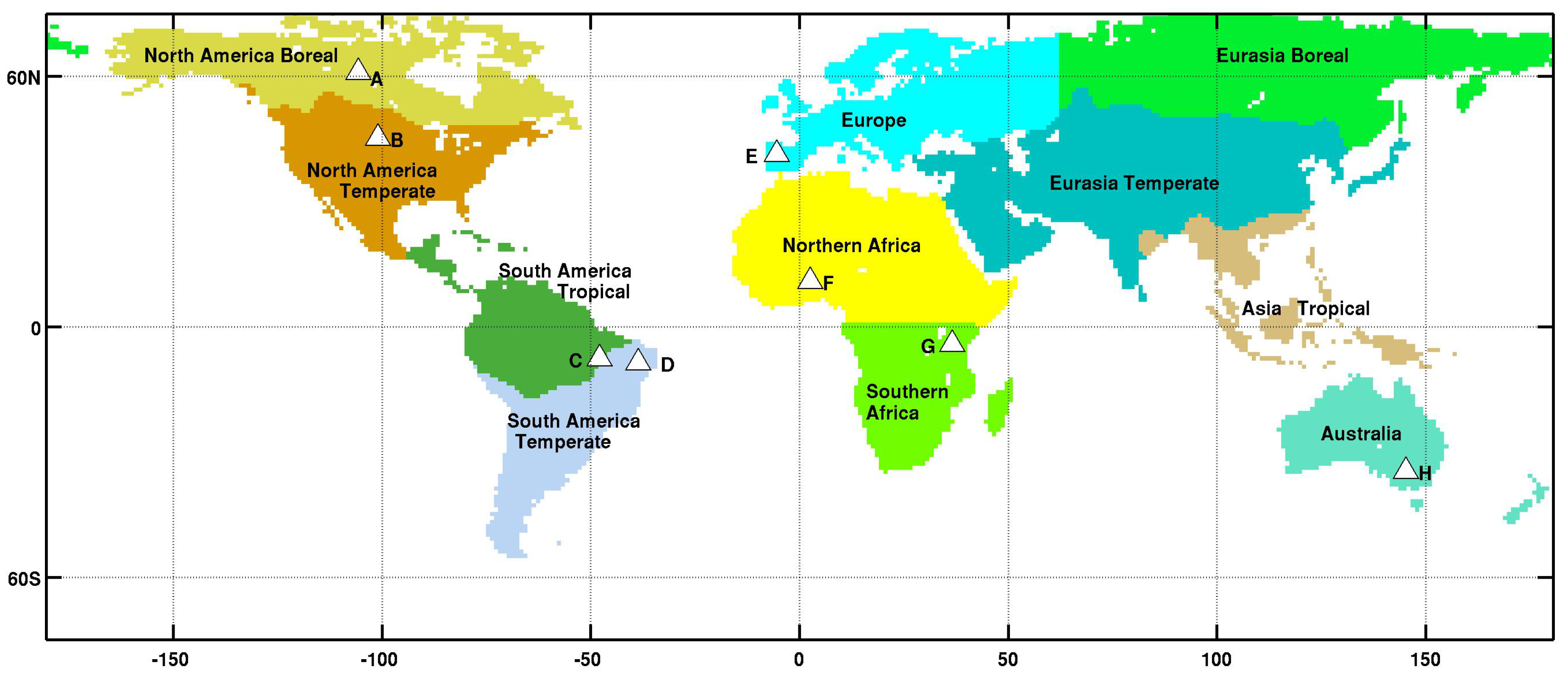
The 11 terrestrial Transcom regions were used as an initial segmentation of global continental land from where to select representative sites. Transcom regions are based on a 1-degree land cover map and are delimited by climate zones [30]. The advantage of using this classification is that it encloses climates with similar vegetation seasonality into a limited number of classes. After careful analysis of the SMOS SM time series in each region, eight target sites were chosen covering Transcom regions North America Boreal, North America Temperate, South America Tropical, South America Temperate, Europe, Northern Africa, Southern Africa, and Australia. No target sites were chosen from Transcom regions Eurasia Boreal, Eurasia Temperate and Asia Tropical, since availability of SMOS SM data in these regions is very limited due to combined effects of RFI, the presence of snow and high topography. A global map showing the selected target sites and the terrestrial Transcom regions is shown in Figure 1. The specific location of each target site is provided in Table 1. One of the SMOS and SMAP Core Cal/Val sites (REMEDHUS, site E) was chosen as a target site for further analysis vs ground-based measurements.
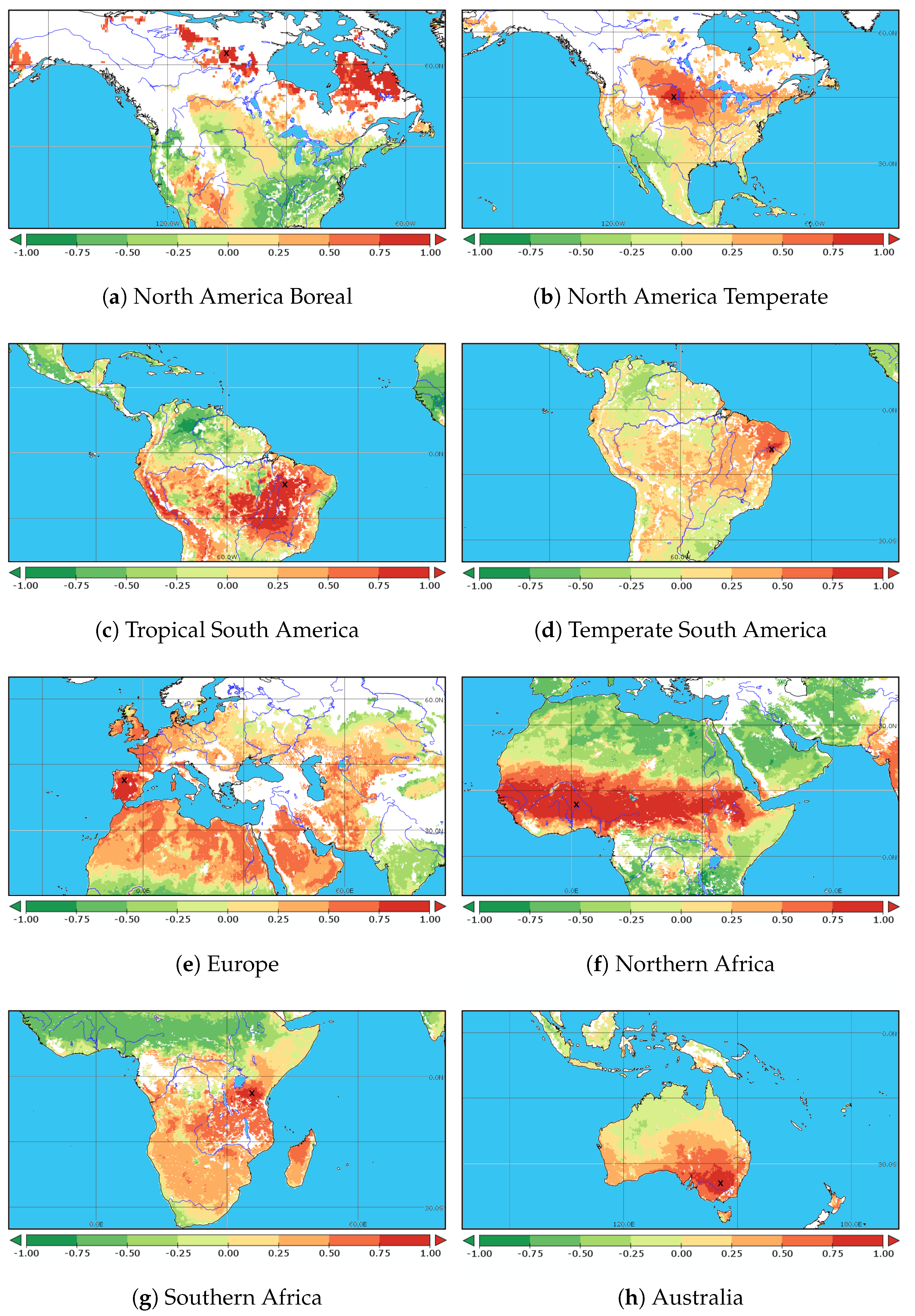
To establish the actual spatial representativeness of the target sites, a temporal correlation analysis was performed at each selected location. Figure 2 shows, for each target site, the correlation map of its SMOS SM time series with the SMOS SM time series of all the pixels on the globe. It can be seen that the highest correlation is located in the neighborhoods of the chosen pixel (within the Transcom Region), which indicates the target site is representative of their surrounding area, but, as expected, not of the whole region.
2.3. Modeled Soil Moisture
2.3.1. GLDAS-Noah
Global Land Data Assimilation System (GLDAS) Noah model v.1 top 10 cm soil moisture estimates were used in this study [31]. GLDAS-Noah land surface state and flux products are provided by the Hydrology Data and Information Services Center (HDISC), a component of the NASA Goddard Earth Sciences Data and Information Services Center (GES DISC). GLDAS-Noah is available with a 3-h temporal interval and 0.25 spatial resolution, covering dates from 2000 to the present. Data was extracted for the eight selected target sites (see Figure 1) and the 6-year study period. The original unit of GLDAS-Noah SM is kg·m, which was converted to volumetric SM (m·m) for this study by considering a top soil layer depth (10 cm) and assuming the density of water in the soil is 1000 kg·m. After averaging for daily values, 1-day time series were used to construct 18-day temporal average fields every 5 days (the rationale for this filtering is explained in Section 2.5).
2.3.2. ERA5
ERA5 is the most modern reanalysis produced by ECMWF, using a recent version of the ECMWF Integrated Forecasting System. The data cover the Earth on a 30 km grid and resolve the atmosphere using 137 levels from the surface up to a height of 80 km. It uses a vast number of observations, including several reprocessed datasets [32]. Although ERA5 is currently in production, the data for the period of this study is already available; top 7 cm soil moisture fields have been extracted for the selected target sites and the 6-year study period. After averaging 00 UTC and 12 UTC to obtain the daily values, 1-day time series were used to construct 18-day temporal average fields every 5 days.
2.4. Ground-Based Soil Moisture
In-situ soil moisture from REMEDHUS (target site E, see Figure 1, Table 1) was obtained through the International Soil Moisture Network [33]. The REMEDHUS soil moisture monitoring network is composed of 23 automated stations deployed within an area of 1300 km in a semi-arid sector of the Duero basin in Spain. Each station is equipped with capacitance probes providing hourly measurements over the top soil 5 cm with a reported accuracy of 0.003 mm. This network has been continuously operating and quality-controlled since 2005 and is therefore ideally suited for validation of multi-year satellite time series. Further details on the network can be found in [12]. For the period of study, data from 17 REMEDHUS stations were available. Data from these stations was first daily averaged and then used to construct 18-day temporal average fields every 5 days (see Section 2.5).
2.5. Temporal Averaging and Filtering of SMOS Data
SMOS L3 daily SM maps need to be pre-processed to ensure smooth spatio-temporal transitions and representative soil moisture states in the climatology. To this aim, outliers were first detected and screened out from the 1-day maps. This was done by comparing the SM retrieved at each pixel with the retrievals embedded within the one-degree box centered at the considered pixel. Any pixel value failing to pass the Tukey outlier test [34] were removed from the dataset. In the next step, the filtered 1-day SM maps were used to construct 18-day temporal average fields every five days. Although the daily SMOS SM maps are useful for the monitoring and evaluation of episodic events, we opted for an average period of 18 days to increase the spatial coverage of the resulting maps, reduce random retrieval errors and filter out high-frequency modes that can be considered as noise when calculating climatological averages. The temporal window of 18-day is the closest to SMOS repeat cycle and the one generally chosen to avoid orbital artifacts (e.g., [35]).
As shown in detail by Robock et al. [36], there are two distinct scales that determine the variations of SM in time and space. The small scale, referred to as hydrological or land surface related scale, is on the order of days and tens of meters. Soil moisture can vary on this scale due to variations of soil properties, vegetation, and topography or drainage patterns. This small-scale variability is intertwined with a much larger scale on the order of weeks-to-months and tens-to-hundreds of kilometers that is mainly due to atmospheric forcing. Microwave satellite measurements integrate over relative large-scale areas on the order of ∼25 km with a typical revisit of 3-days. At these spatio-temporal scales, the short-term (up to 3 days) and small-scale (tens of meters) land surface component of soil moisture variability appears as random (white) noise in comparison with the long-term (about 1–4 months) and large-scale (about 400–800 km) signal related to atmospheric forcing.
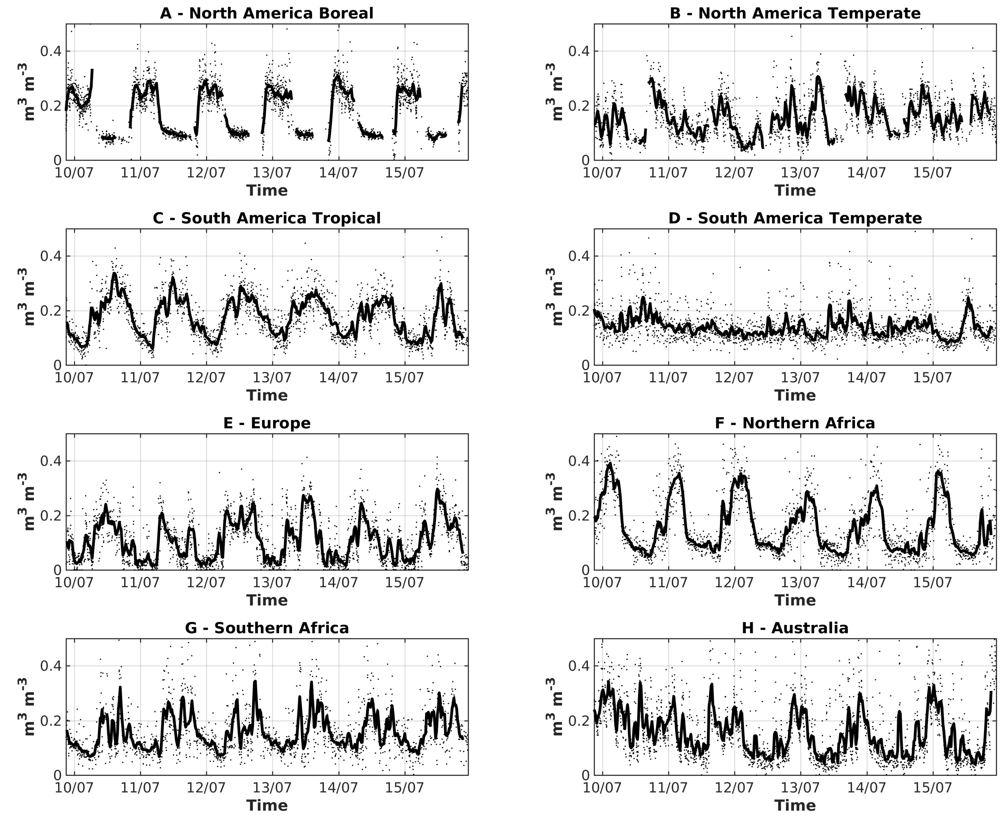
Examples of the time series of the original 1-day SM, together with the 18-day average, are shown in Figure 3 for the 8 target sites, which cover a variety of vegetation seasonality and climatic conditions (Figure 1, Table 1). Dots represent the daily values and the solid line corresponds to the 18-day average every five days. It can be seen that the variability of the daily signal is captured in the filtered time series, where the six SM annual cycles can be clearly identified. Difference in magnitude and extent of rainy seasons among years are more clearly distinguished in the filtered series (e.g., sites E and H). Also, notice the opposite timing of wet and dry seasons in Northern and Southern Africa (sites F and G), which reflect the displacement of the Inter-Tropical Convergence Zone (ITZC). Site D exhibits limited temporal variability in both the original and the filtered series.
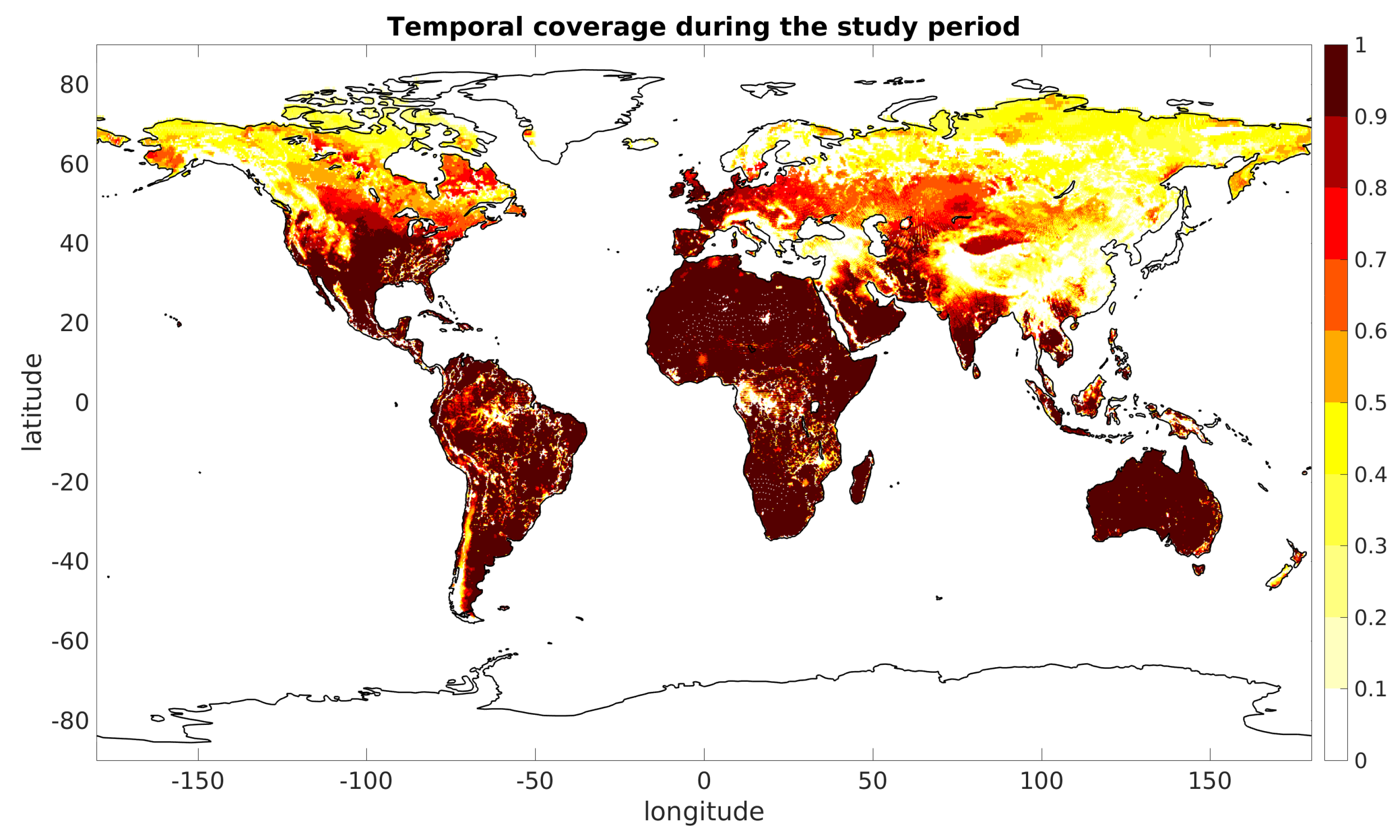
Notice that not all the 25-km pixels in this 18-day averaged SM fields are continuously observed. SMOS’s wide swath (1000 km) and polar orbit allow for a 3-day global revisit period. However, there is an important amount of missing data due to the presence of radio frequency interferences masking L-band measurements, particularly in South-East Asia [27]. In addition, no retrievals are attempted in areas of high topography (e.g., Himalaya) and in soils covered by snow. The latter strongly reduces the data availability in high latitudes and especially during the fall and winter seasons. The global map of Figure 4 shows the SMOS temporal coverage for the study period, with 1 representing a 100% coverage of the filtered and temporally-averaged SMOS signal. In this study, only the pixels with a minimum of 80% temporal coverage were used in order to ensure representativeness and robustness of the signal decomposition and of the results presented. As we will show later in the study, this threshold does not exclude areas with limited data in winter due to snow. The impact of these “intermittent” data gaps in the STL decomposition is discussed in Section 3 and Section 4.
2.6. Signal Decomposition
The STL geostatistical procedure is used in this work to decompose the SMOS signal into its temporal components and build an observation-based SM climatology. The STL technique was originally introduced by Cleveland et al. [25], and adapted by Humphrey et al. [37] to evaluate the seasonal cycle of unevenly spaced time series using locally weighted regression, or Loess. This technique has already been used in several research studies to extract the seasonal and interannual components of GRACE time series [37,38,39]. In this work, the STL procedure has been used to decompose the filtered and temporally-averaged SMOS SM signal () as the sum of a seasonal component (), a low-frequency component () and remaining high-frequency residuals ():
The low-frequency component contains only periodicities larger than a season and is further decomposed into linear trends () and the anomalies with respect to this linear trend or interannual variability (). The high-frequency residual is expected to be both a real signal representing subseasonal variability and noise present in SMOS data. For a detailed description of the method, refer to [25,37]. In short, STL is a double recursive approach: an inner iteration cycle is used to recover the seasonal cycle from the low-frequency component using Loess; the outer iteration cycle is used to recalculate the Loess weights and to separate the signal between low- and high-frequency components again using Loess. At the end of the process, the low-frequency signal remaining after removal of the seasonal cycle is decomposed as a trend and an interannual signal. The residual component is equal to the resulting high-frequency component.
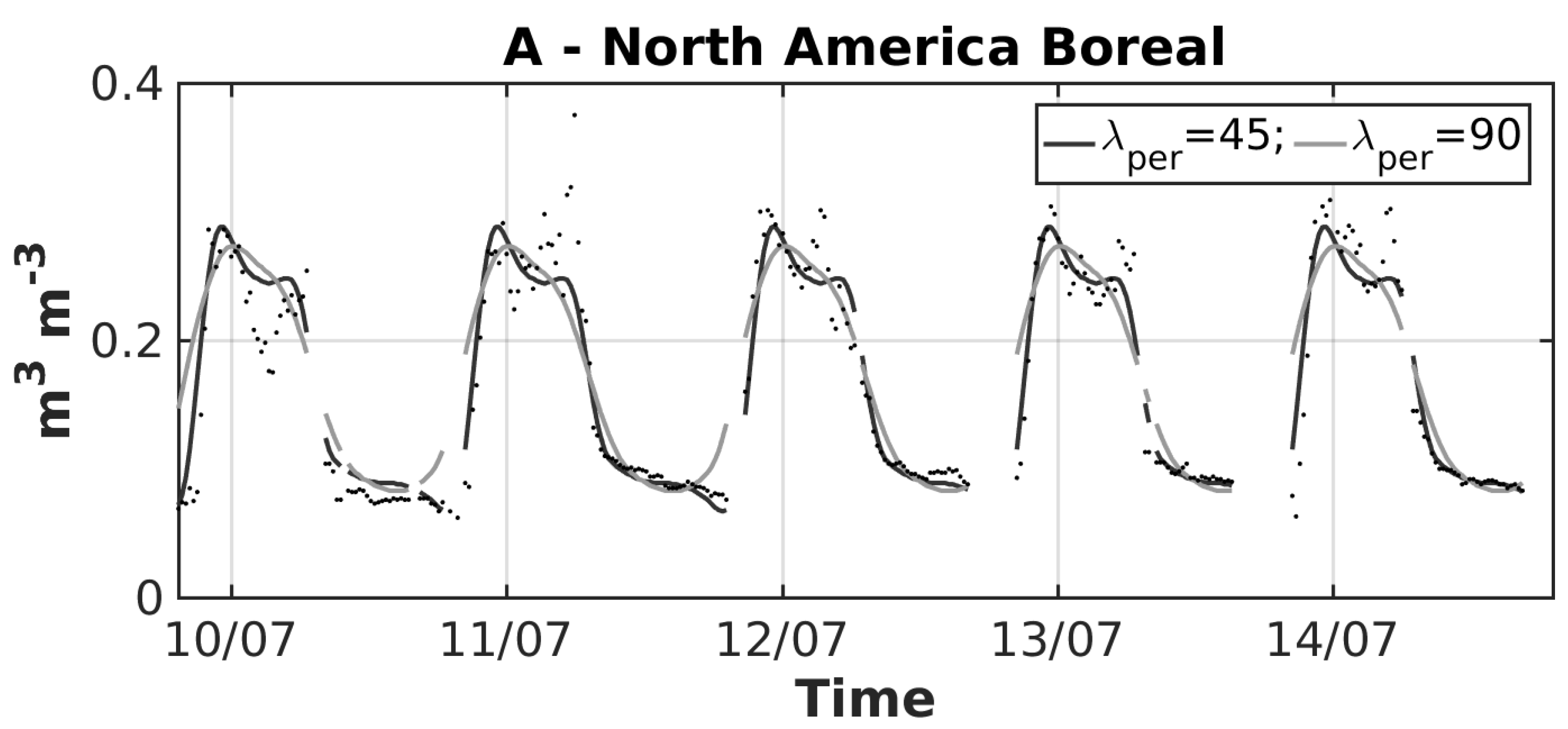
The application of the STL algorithm requires the specification of six smoothing filter parameters that need to be optimized to minimize spectral leakage between high- and low-frequency components and control the possible influence of outliers in the time series. These are: (1) the length of the seasonal cycle; (2) the degree of the weighted polynomial regression; (3) the number of cycles of the inner loop (used to estimate the trend, the seasonal and the interannual components); (4) the number of cycles of the outer loop (used to estimate the residual signal, i.e., the subseasonal component); (5) the maximum time lag for the seasonal component, and (6) the maximum time lag for the long-term component. Here, the seasonal cycle is taken as exactly 365 days, a multiple of the 5-day map interval (which was constructed disregarding the occurrence of the leap day, 29 February 2012). Following Humphrey et al. [37], the number of inner and outer loops is set to 2 and 3, respectively, a quadratic fit is used for the seasonal cycle and a linear fit for the long-term components. The optimal values for the maximum time lag of the seasonal and long-term components have been selected after a comprehensive analysis carried out at the 8 target sites that is reported hereafter. The role of the maximum time lag for the seasonal component is illustrated in Figure 5 for site A. It is shown that the smoothness of the seasonal cycle increases with the value of the maximum seasonal time-lag period. Although large values are recommended when using noisy data, they may hide key details of the seasonal cycle. A maximum seasonal time lag of 90 days fails to reconstruct the double-maximum SM in June and September. Instead, it results in an erroneous maximum during July. On the other hand, too short maximum seasonal time lags tend to over fit the noisy data. A similar effect was observed for sites C, E and G, whereas there was not a strong impact in B, D and F (not shown). These results indicate that a maximum seasonal time lag of 45 days is a reasonable compromise for SMOS SM data and it is the value used for the rest of this study.
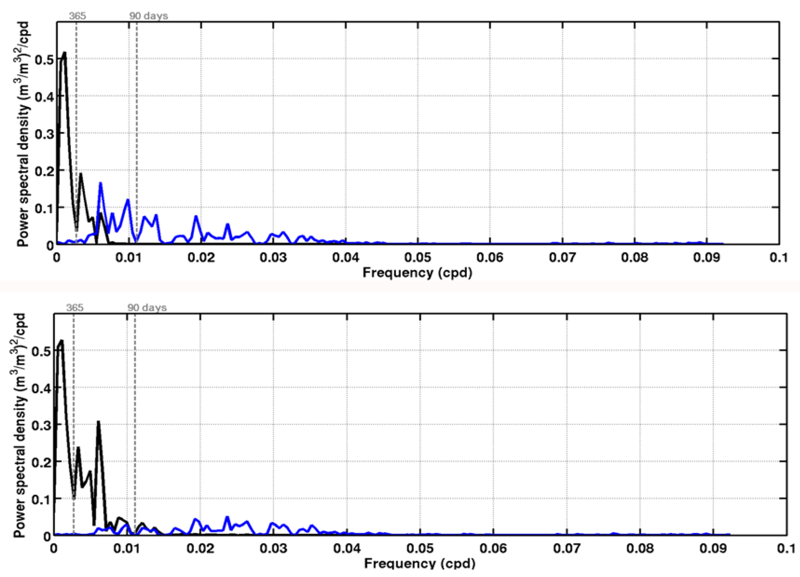
The role of the maximum time lag for the long-term or low-frequency component is to separate the seasonal anomalies between a low-frequency (that will be further decomposed as a trend and an interannual component) and a residual high-frequency component. Figure 6 shows the spectra of the interannual and subseasonal SM components for a long-term maximum time lag of 0.20 × 365 (top) and of 0.10 × 365 (bottom). It is observed that the larger lag leads to a subseasonal component having maximums for cycles beyond 90 days, whereas the shorter lag leads to a subseasonal variability closer to white noise. Here, the lag of 0.10 × 365 has been selected since it allows a more appropriate decomposition of long-term variability and residual components (which integrates both subseasonal variability and instrumental noise). Results shown in Figure 6 are for site A, results obtained for the other sites are consistent (not shown).
2.7. Analyses at Target Sites
The STL procedure was applied to the SMOS time series at the target sites. The obtained distribution of SMOS SM variance among its temporal components was analyzed in detail. Subsequently, SMOS, GLDAS-Noah and ERA5 SM time series at these locations were inter-compared to identify consistencies and potential shortcomings of building a climatology with satellite data alone. A comparison of the three data sets to ground-based SM was performed for one of the target sites (REMEDHUS, in Europe). Statistical scores of the comparisons are provided.
2.8. Analyses at the Global Scale
Global maps of the long-term average and standard deviation of SM were computed on a pixel basis over the filtered and temporally-averaged SMOS signal. The STL decomposition was subsequently applied globally to each individual pixel with a temporal coverage greater than 80% for the study period (see Figure 4). The relative magnitude of the extracted long-term, seasonal and residual components with respect to the total variance was computed to assess the dominant modes of temporal variability in global SM during the study period. The magnitude of the linear trends within the long-term component were also evaluated per pixel at the global scale.
3. Results
3.1. Soil Moisture Temporal Decomposition at Target Sites
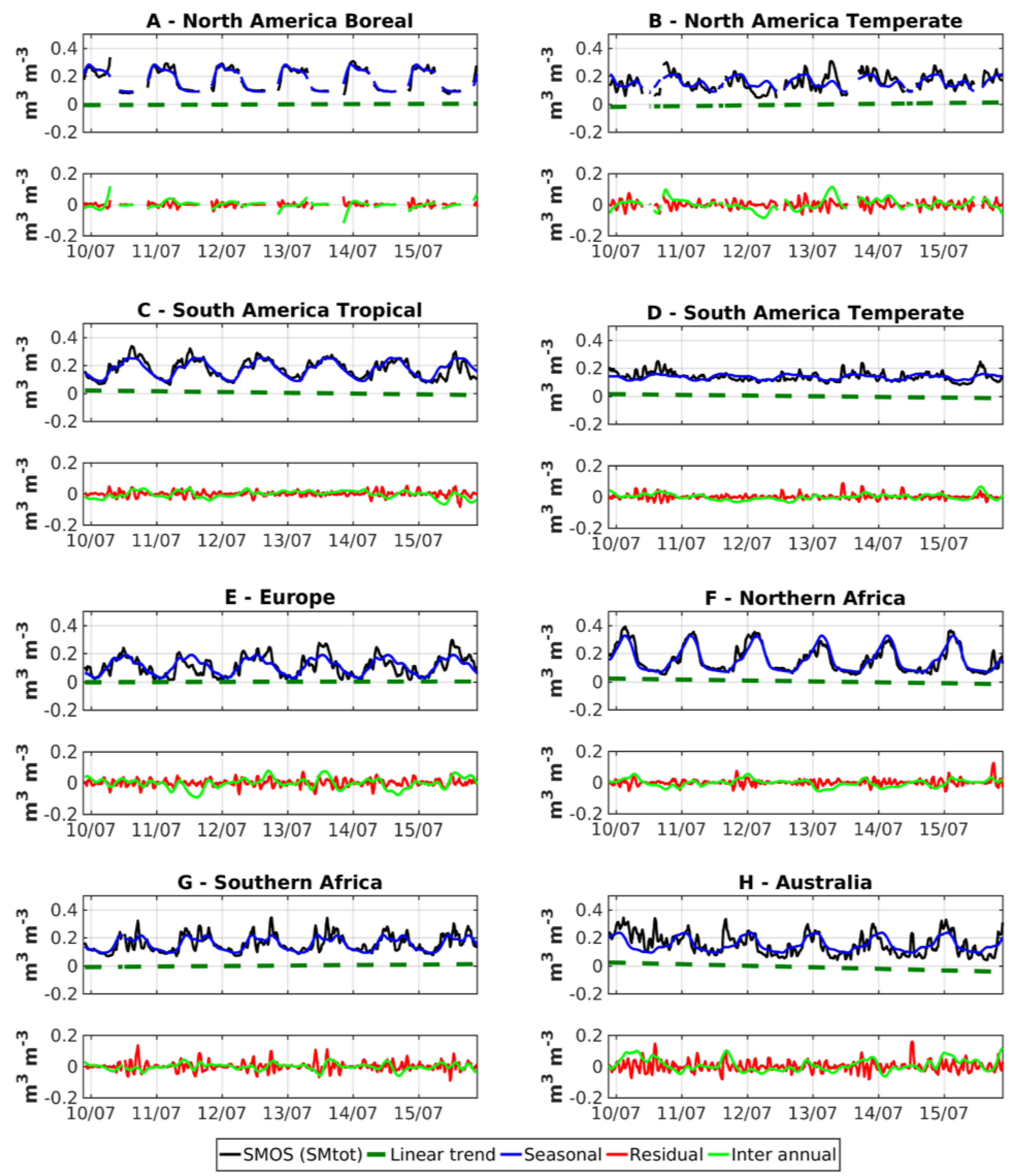
Figure 7 illustrates the STL decomposition of the SMOS signal into the different subcomponents at the 8 target regions. In general, the temporal series show an almost negligible linear trend, with Australia (H) and South America Temperate (D) presenting a slight trend towards drier conditions and North America Temperate (B) and Southern Africa (G) revealing a slight trend towards wetter conditions. This will be examined in detail later in this section. A clear seasonal signal is extracted for most of the sites, except for South America Temperate (D), which exhibits limited temporal variability in the original series (see also Figure 3). The residual component shows a temporal behaviour similar to that of white noise in all the sites. It is especially high in Australia (H) and, to a lesser extent, in Southern Africa (G). The analysis for Europe (E) reflects a regular seasonal cycle, with exceptionally dry conditions in winter of years 2011–2012 and 2014–2015, and exceptionally wet conditions during short periods of spring 2012, winter 2013–2014 and end of 2015, as suggested by the analysis of the interannual component. The dry anomaly in winter 2011–2012 has also been reported in previous studies devoted to detection of agricultural drought [40,41]. The interannual component presents also prominent fluctuations in North America Temperate (B), Southern Africa (G) and Australia (H). In particular, the dry anomaly observed in North America Temperate (B) in 2012 reflects the strong summer drought suffered in the contiguous US due to unusual high temperatures in spring and summer 2012 combined with record low rainfall [42]. The analysis of North America Boreal (A) exemplifies the non-negligible impact of temporal gaps in the decomposition procedure. The wet peak measured by SMOS in October 2010 and followed by a short no-data is assigned mainly to the subseasonal component. The same applies to the wet peak measured in October 2013, which is not affected by the absence of data. In contrast, there is a no-data corresponding to the winter months of the six annual cycles that are assigned to the interannual component. This reveals a limitation of the method to correctly differentiate short-term from long-term variability in the extremes of temporal gaps. This same effect was observed in initial tests conducted at target sites within Eurasia Boreal, Eurasia Temperate and Asia Tropical (see Figure 1), which were discarded from the analysis. Although we imposed an 80% minimum temporal coverage, the impact of no data in the time series needs to be taken with some caution when interpreting overall results.
3.2. Comparison of SMOS, GLDAS-Noah, ERA5 and In-Situ at Target Sites
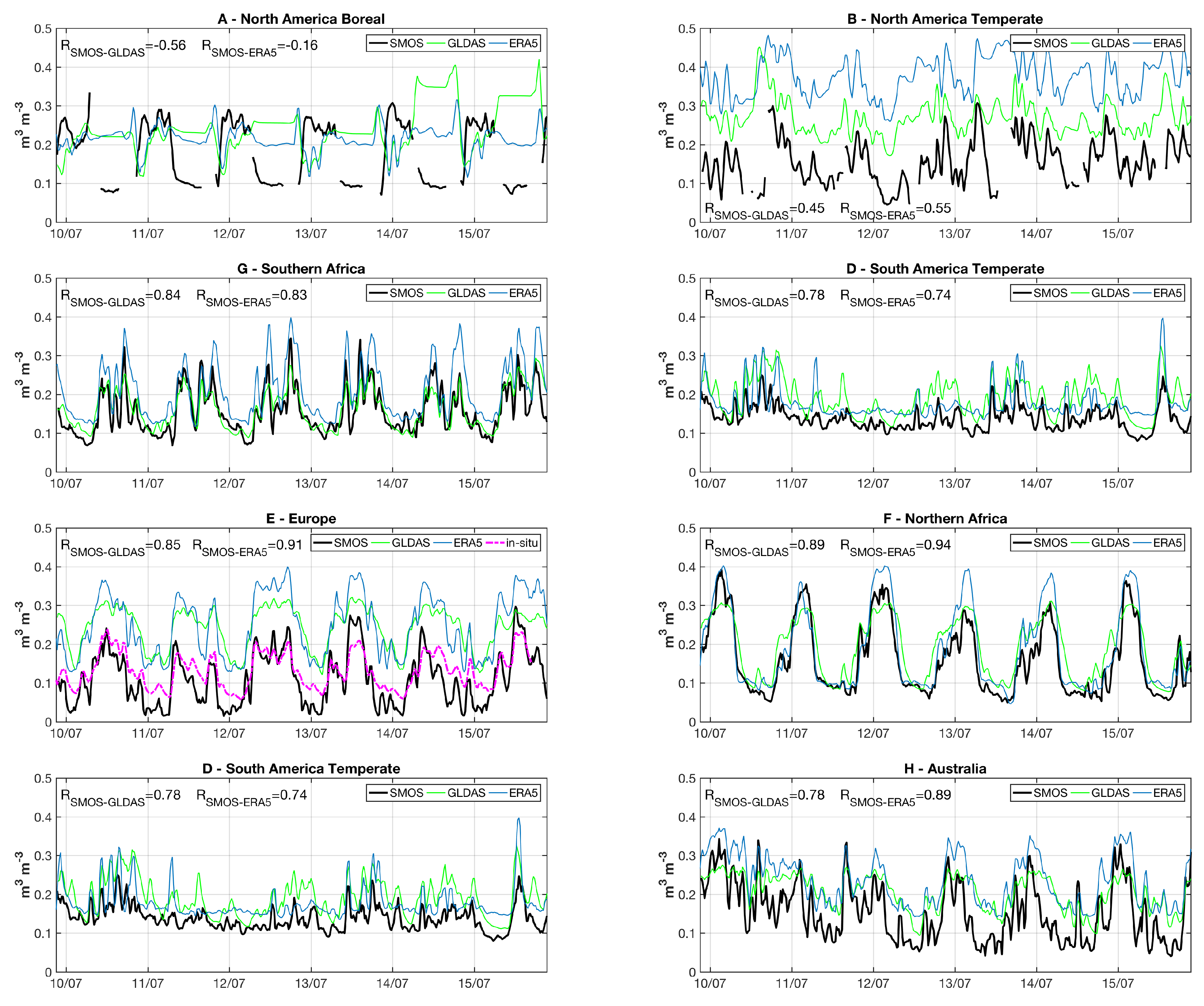
Time series of SMOS-based SM together with top 10 cm soil moisture GLDAS-Noah and top 7 cm soil moisture analysis from ERA5 are shown in Figure 8. It can be observed that in regions C to H, SMOS, GLDAS and ERA5 soil moisture time series are comparable in terms of temporal phase (Pearson correlation of 0.7–0.9). In regions A and B, however, the SMOS observations are uncorrelated with the uppermost soil moisture modeled estimates. This is mostly due to the presence of snow, which masks satellite measurements and can also affect the uncertainty of model predictions. Further research is needed in these areas of mutual disagreement to identify potential deficiencies in the satellite and/or in the model estimates. Similar results were reported by a previous study comparing SMOS with MERRA reanalysis [43]. Note that the correlation metric benefits from the seasonal cycle, which for the period of this study is included. Correlation of time series at daily time scales lead to similar results (not shown).
There are notable differences in the absolute values of satellite and modeled data (e.g., sites E and H), which remarks the need to use bias correction procedures when assimilating soil moisture satellite observations in land surface simulations [44]. The assimilation of satellite data in land surface models has proven to be a powerful technique to leverage from the two sources of information. A recent study has shown that assimilating SMOS SM data into the Noah Land Information System after bias correction significantly increased the anomaly correlation of modeled top soil moisture estimates with station measurements [45]. Also, Pinnington et al. [46] showed that assimilation of (bias-corrected) satellite rainfall and SM data had the greatest impact on model estimates during the seasonal wetting-up and drying-down of the soil, respectively. While L-band satellites have been designed for measuring soil moisture, land surface models have been designed for a much wider purpose, including ecological, hydrological or climate applications. Modeled soil moisture is generally highly sensitive to the meteorological forcing data used and the land surface model encoded physics [47,48]. This makes comparison of absolute values of observed and modeled SM very challenging, and therefore studies generally focus on the comparison of SM temporal anomalies (e.g., [19,20]), or even in the comparison of observed and modeled brightness temperatures directly (e.g., [49]). The differences found between modeled and observed SM and also among different models support the idea proposed here of leveraging from the natural soil moisture variability captured by satellite observations as a reference for harmonizing SM climate data records so that they become model-independent.
Ground-based soil moisture data from REMEDHUS (average of 17 in-situ stations) are also included in Europe time series (Figure 8E). It can be seen that both satellite and models generally capture the temporal dynamics measured by the in-situ sensors. A statistical analysis has been undertaken following the recommended performance metrics in [50]. Results are shown in Table 2. The temporal correlation (R) and the unbiased Root-Mean-Squared difference (ubRMSD) between the in-situ, remotely sensed and modeled SM are satisfactory (R > 0.85, ubRMSD < 0.003). As in the previous analyses, it should be noted that the R metric benefits from the seasonal cycle, which for the period of this study is included. In terms of accuracy, SMOS shows a low dry bias of 0.02 while the two models present a large wet bias of about 0.11 mm. As expected, the models capture reasonably well the temporal dynamics but not the absolute magnitude [47]. The statistical scores when calculated at daily time scales lead to similar results (not shown).
3.3. Temporal Mean and Variance of SMOS Soil Moisture Retrievals at the Global Scale
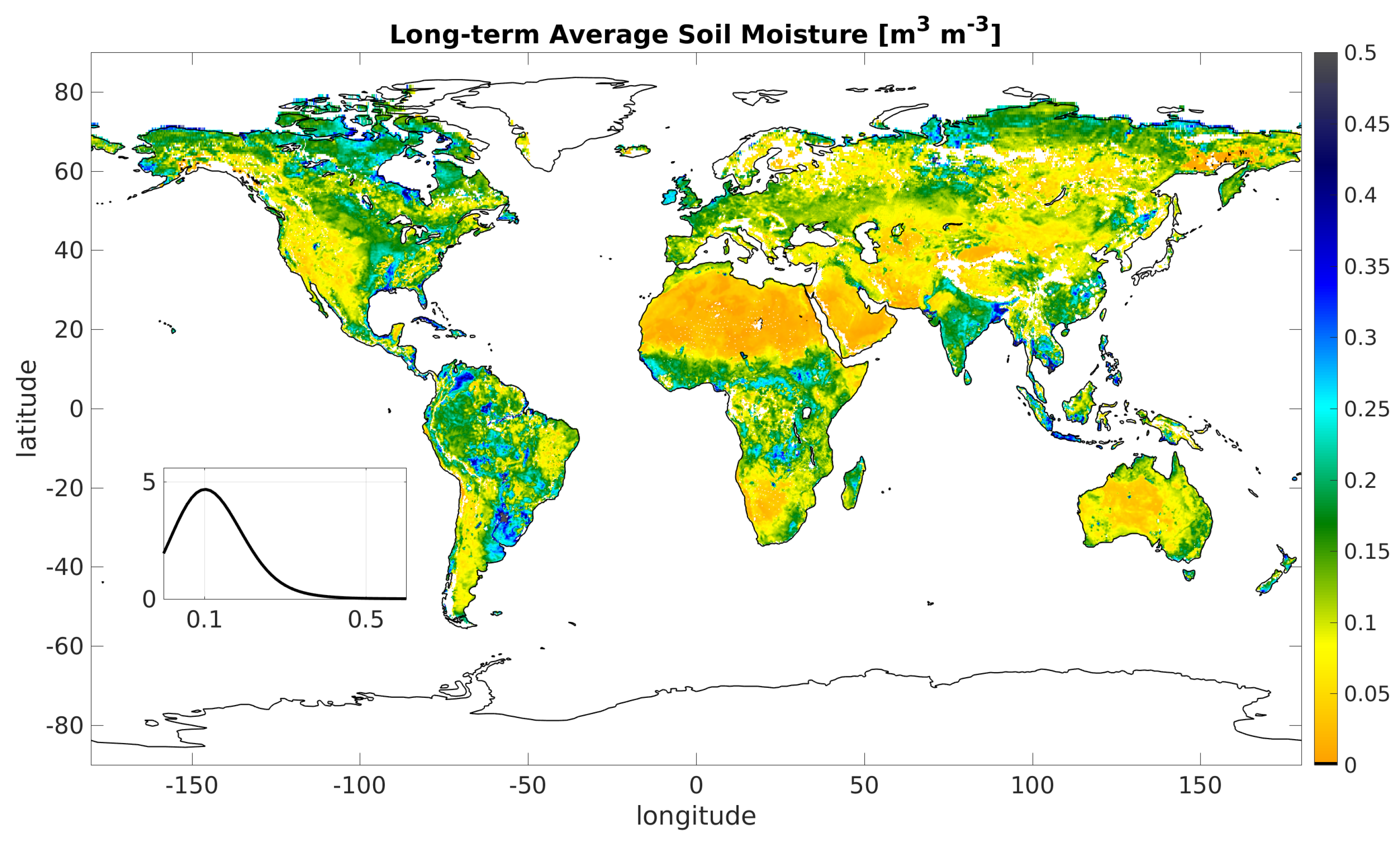
The temporal average global map of SMOS SM surface volumetric soil water content for the study period (pixel average of in Equation (1)) is shown in Figure 9. The average conditions observed during the study period exhibit a mode of 0.1 mm (inset figure). It shows the expected spatial patterns of SM, from the dry arid regions to the wet forested areas. Note that the average conditions shown in areas with limited availability of data may not be representative (e.g., northern latitudes and tropical Africa, see coverage map on Figure 4).
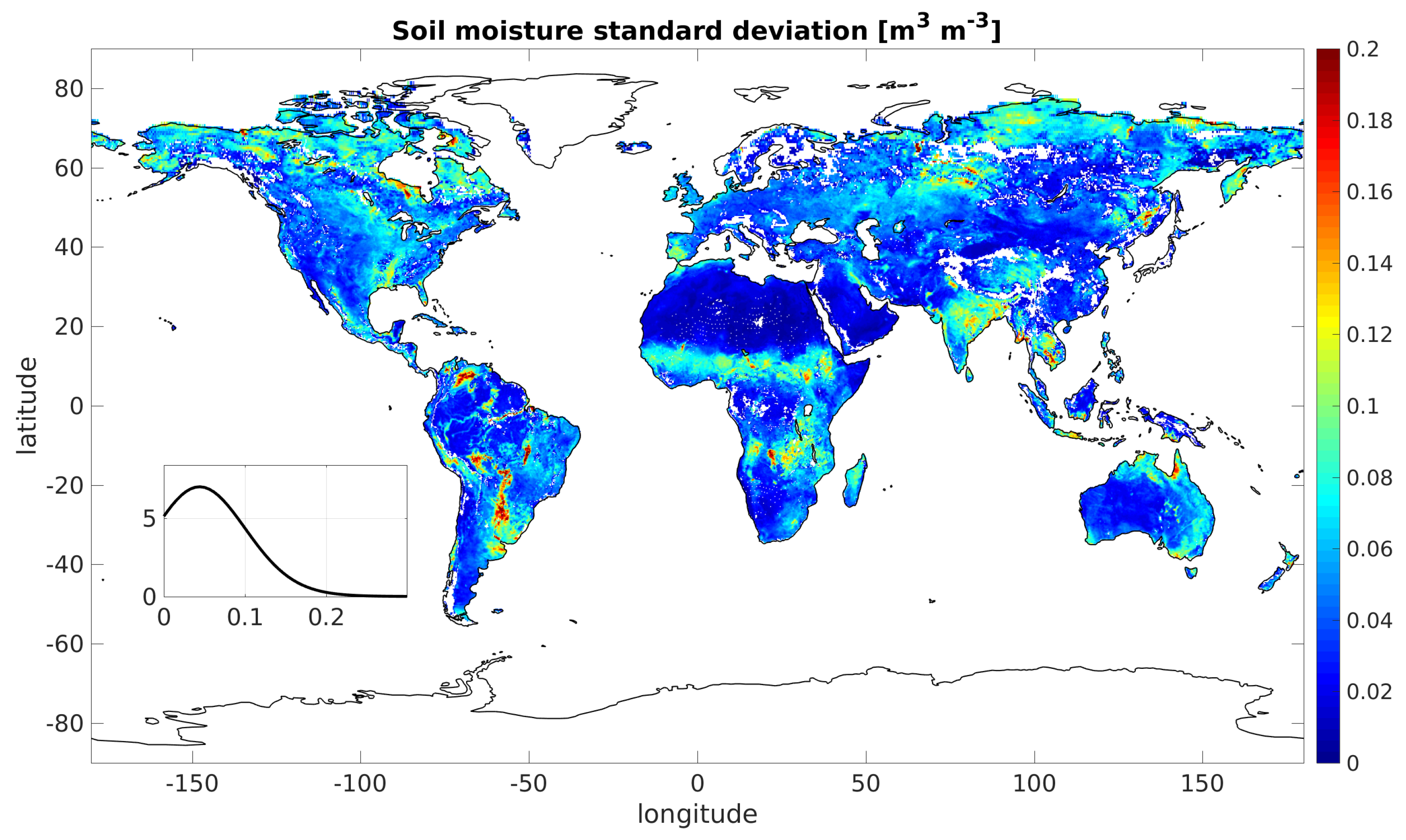
The global map of SMOS SM standard deviation for the study period (standard deviation of in Equation (1)) is shown in Figure 10. As expected, areas with higher variability are concentrated in the tropics, where there is a strong seasonality dominated by the position of the ITCZ [51]. Other areas with strong variability include India and South-East Asia, strongly affected by Monsoon rainfall, and some regions in the Southern Hemisphere like eastern Australia and South America that could be related to ENSO. In particular, the high SM variability observed in the so-called Southeastern South America (SESA) region can be explained by the intense summer precipitation over this region [52]. This pattern has also been observed with satellite SM products derived from higher microwave frequencies and climate models [53], and responds to strong land-atmosphere interactions in the region. The variability observed in northern latitudes is probably due to imperfect detection of ice/snow and poor temporal coverage (see Figure 4).
3.4. Analysis of the Dominant Features of Global Soil Moisture Variability
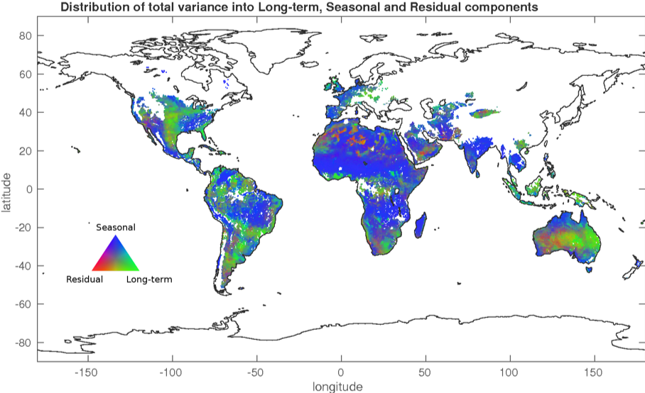
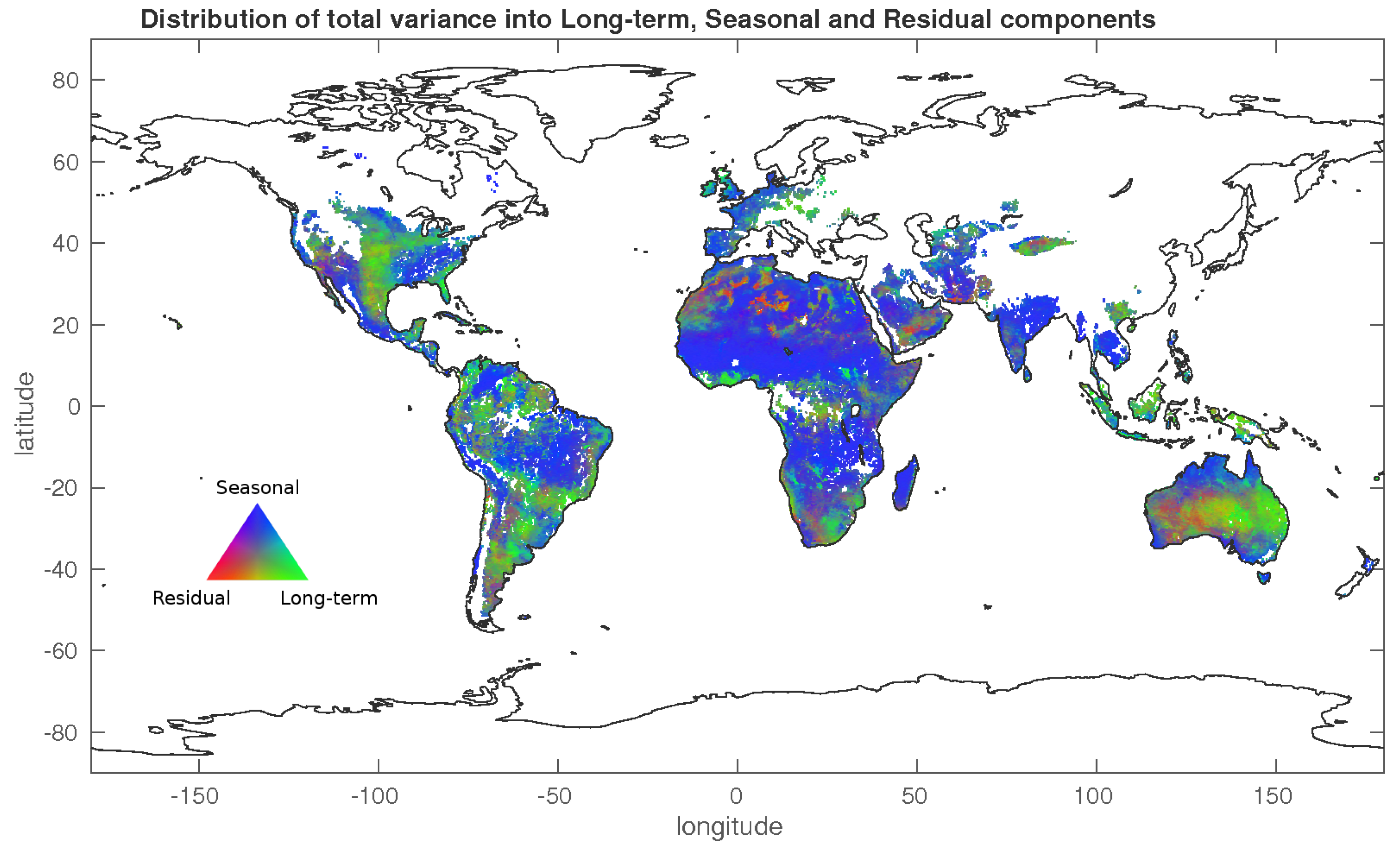
In this study we decomposed the total variance of the soil moisture signal (Figure 10) by breaking it down into: (1) a seasonal component, (2) a long-term component, and (3) a high-frequency residual or subseasonal component. The relative magnitude of each of these three components is shown as an RGB triplet in Figure 11. It reveals the seasonal cycle is dominant in many tropical regions such as Brazil, Central Africa, India and Northern Australia. Wet tropical forests such as the Amazon and Congo exhibit high spatial heterogeneity in its dominant components, probably due to the combined effects of human activities and climate variability. In contrast, the soil moisture variability in dry tropical forests, including the savannahs south of Central Africa and several regions in Southwestern Brazil, is clearly dominated by seasons. Though dry tropical forests may receive several hundred centimeters of rain per year, they have long dry seasons which last several months and vary with geographic location. Forests in dry tropics show great diversity of phenological patterns and large interannual variation, with predominance of deciduous tree species [54]. Our analysis indicates that L-band is capturing the emissivity from the soil and the seasonal drought through the forested canopy. Two regimes can be identified in Europe: whereas western countries are governed by seasonal variability, long-term variability predominates in the eastern countries. In Australia, seasonality dominates the north and the south-east, the eastern region is dominated by long-term variability and the western by subseasonal. The Indo-Australian archipelago is also dominated by long-term variability. It is interesting to note that subseasonal variability is predominant in regions where the SMOS signal has already a relatively low variance (Figure 10) and is most likely influenced by noise such as the Sahara desert, the Arabian Peninsula and Western Australia, i.e., where the noise is at least of the same magnitude that the annual variance. Indeed, despite having carefully filtered the data, some of the SMOS retrievals in Asia and Europe may still be affected by undetected RFI contamination [27]. Also, results may be affected by the intrinsic uncertainty of microwave satellite SM retrievals, which is higher in presence of dense vegetation canopies, heterogeneous landscapes, and high topography [6,11,55].
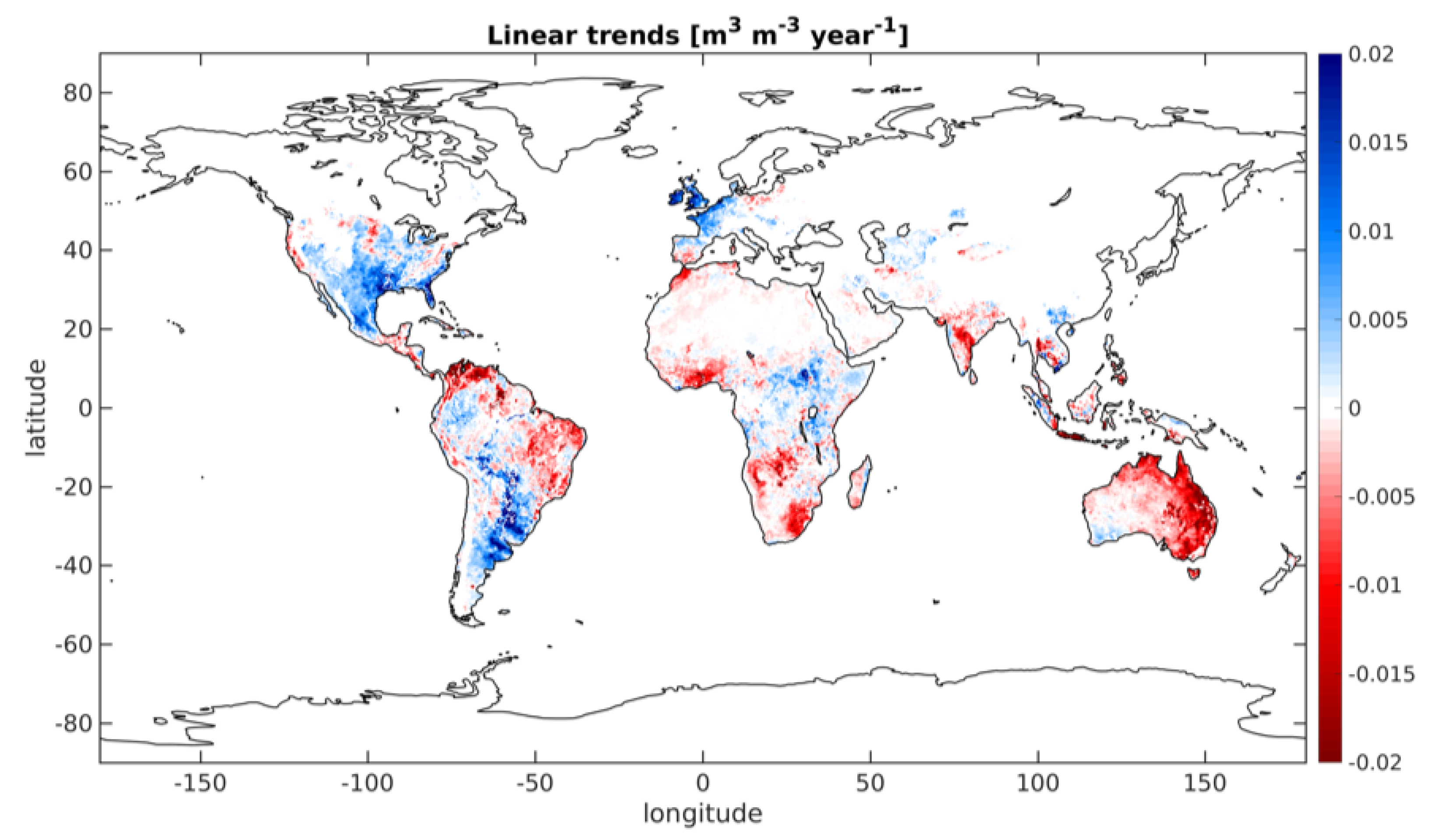
The linear trends within the long-term variability component are further examined in Figure 12. The linear trends observed in the SMOS signal illustrate the ENSO conditions during the six-year study period. During the first five annual cycles -from 2010 to 2015- the equatorial Pacific Ocean was mostly in a cold phase (La Niña); however, a warm event (El Niño) occurred during the last cycle (i.e., in 2016). This explains why SMOS-derived linear trends reproduce known ENSO teleconnection spatial patterns. During El Niño, limitations in terrestrial moisture supply result in vegetation water stress and reduced evaporation in eastern and central Australia, southern Africa and Eastern South America (areas in red). The contrary situation is experienced in Argentina, Tanzania and southeastern US (areas in blue), where there is a regime of above-average rainfall. This result is in line with a previous study that showed that multi-decadal (1980–2011) variability in SM and terrestrial evaporation was dominated by ENSO dynamics [56]. The linear trends in Figure 12 also provide evidence of strong dry/wet patterns in regions which have not been previously related to ENSO precipitation patterns (e.g., western Europe, Northern Africa, California). Still, results should be taken with caution, and further analysis of the long-term variability is needed to identify new climate patterns at short and median temporal scales. Investigating the relation of ENSO to global soil moisture variability and the existence of potential new teleconnection patterns is recommended for future research.
4. Discussion and Final Remarks
The two first space missions dedicated to measuring the Earth’s surface soil moisture have been launched in the last decade: SMOS in 2009 and SMAP in 2015. They are providing L-band measurements that, combined with C- and X-band measurements available since the 1980s, allow generating, for the first time, observational soil moisture climate data records combining the three microwave frequency bands. However, the synergies of microwave measurements across different frequencies and the potential of the L-band data record to serve as a common reference to harmonize the long-term data record have not yet been fully exploited. This study presents first evidence that the relatively short data record of available SMOS L-band observations allows characterizing the main modes and spatial distribution of the Earth’s surface soil moisture variability. This information could serve as a reference to harmonize and construct a model-independent SM climate data record. In its current version, the ESA CCI soil moisture product uses a climatology obtained from GLDAS-Noah to harmonize the individual products for the 40-year period of record. However, given the differences found between modeled and observed SM, and among SM from different models, there is a clear need for a SM climate data record based solely on observational data sets. Such a record will be instrumental to verify land surface model performance and trends.
This study is a first attempt to derive a global L-band climatology from observational data alone. The STL geostatistical procedure was implemented and tailored to the first six annual cycles of SMOS data to decompose the temporal variability of the signal. For the period of study (2010–2016) this analysis allowed identifying regions where soil moisture variability was dominated by seasonal cycles, regions that did not exhibit a clear seasonal pattern and with likely subseasonal variability, and regions where the long-term variability dominated. Results show that the seasonal cycle was dominant in the tropics (Brazil, Central Africa, India and Northern Australia), and in dry tropical forests, including the savannahs south of Central Africa and several regions in Southwestern Brazil. Wet tropical forests, in turn, exhibited high spatial heterogeneity in its dominant components, probably due to the combined effects of human activities and climate variability. In Europe, western countries were governed by seasonal variability whereas the long-term variability predominated in the eastern countries. In Australia, seasonality dominated the north and the south-east and the eastern region was dominated by long-term variability. Interestingly, in regions where SMOS has very limited variance (e.g., Sahara desert, Arabian Peninsula, Western Australia), the subseasonal or residual component was dominant. This is probably due to the fact that the noise of the observations is at least of the same magnitude that the annual variance and the dominant variability is identified as noise. During the study period (2010–2016), the equatorial Pacific Ocean was mostly in a cold phase until 2015–2016 when there was a transition to a warm phase. The observed global linear trends, based upon the strong El Niño event in 2016, are shown to be consistent with the ENSO teleconnections calculated over multiple events.
This study has demonstrated that L-band observations provide a reliable source of data to monitor the distribution of shallow water content in continental surfaces from space platforms. However, this study cannot conclude on the presence of a clear climate trend in the water content of the soil and results should be taken with caution, since they are limited by the length of the L-band data record available (∼8 years vs. the 30 years which are generally considered for climate studies). Still, our results are consistent with a previous study that showed that multi-decadal (1980–2011) variability in SM and terrestrial evaporation was dominated by ENSO dynamics [56]. Also, there are relevant studies considering the trends of SM and terrestrial evapotranspiration at scales smaller than 30 years (e.g., 10 years in [57]).
Our results showed that the STL procedure, after adequate parameterization, was a solid means to build a soil moisture climatology based solely on the temporal dynamics of the data. Yet, it would be recommendable to assess in future research the additional benefits of using techniques exploiting the temporal and spatial components of the data (e.g., [24,58,59]). The global STL parameterization was thoughtfully chosen after an analysis at 8 selected sites with distinct vegetation seasonality and climatic conditions. However, they do not likely cover each climate on the Earth continents and may not be optimal under specific conditions (e.g., areas where small SMOS variance is dominated by noise). A comparison with modeled GLDAS-Noah and ERA5 soil moisture reanalysis in the selected sites, and with in-situ data at the REMEDHUS site (Europe), provides confidence in the obtained results. The exception is in areas where the presence of satellite data gaps -although limited to 20% of the study period- leads to mutual disagreement of model and satellite estimates. It should be noted that the presence of observational data gaps in the satellite time series can potentially bias the obtained climatology and severely limit the applicability of the method to Northern latitudes, where seasonal snow masks soil emissivity and soil moisture retrievals cannot be performed. In this regard, recent studies on the use of Gaussian process regression techniques to mitigate the effect of missing information in Earth observation data are very promising (e.g., [60]).
This work has shown that the relatively short SMOS data record allows providing insight into the dominant modes of temporal variability in the Earth’s surface soil moisture. Also, although previous studies have shown some weaknesses of SMOS retrievals (e.g., [11,27,55]), the good correlation obtained with ERA5 modern reanalysis and GLDAS-Noah indicates that an L-band climatology, such as the one proposed in this study, is a reasonable reference to be used for a climate data record exclusively based on remote sensing data. The presented SMOS-based climatology offers a unique view of recent processes governing freshwater fluxes in the water cycle, and allows observing specific phenomena, as the different variability regimes present within the Amazon and Congo basins and the dominance of the interannual variability in wide regions within Europe, United States, Eastern Australia and South America. It also opens the path to forthcoming studies focused on the analysis of the interannual variability and the impact of ENSO in areas that have not been documented so far.
Author Contributions
All authors contributed significantly to this research. The initial idea was conceived by M.P. and J.B.-P.; M.P. carried out the data analysis and led the manuscript writing; J.B.-P. implemented the STL decomposition technique and adapted it to SMOS data; J.M.-S. fully contributed to the design and development of the study and provided the ERA5 data. All the authors contributed to the interpretation of the results, participated in the manuscript and approved it.
Funding
This research received no external funding.
Acknowledgments
M.P. is supported by a Ramón y Cajal Contract (Spanish Ministry of Science, Innovation and Universities). The authors would like to thank the support received from the ESA CCI Soil Moisture project team.
Conflicts of Interest
The authors declare no conflict of interest.
References
- Entin, J.; Robock, A.; Vinnikov, K.; Hollinger, S.; Liu, S.; Namkhai, A. Temporal and spatial scales of observed soil moisture variations in extratropics. J. Geophys. Res. 2000, 105, 11865–11877. [Google Scholar] [CrossRef]
- Seneviratne, S.; Corti, T.; Davin, E.; Hirschi, M.; Jaeger, E.; Lehner, I.; Orlowsky, B.; Teuling, A. Investigating soil moisture-climate interactions in changing climate: A review. Earth Sci. Rev. 2010, 99, 125–161. [Google Scholar] [CrossRef]
- Taylor, C.M.; Gounou, A.; Guichard, F.; Harris, P.P.; Ellis, R.J.; Couvreux, F.; De Kauwe, M. Frequency of Sahelian storm initiation enhanced over mesoscale soil-moisture patterns. Nat. Geosci. 2011, 4, 430. [Google Scholar] [CrossRef]
- Koster, R.D.; Mahanama, S.P.P.; Yamada, T.J.; Balsamo, G.; Berg, A.A.; Boisserie, M.; Dirmeyer, P.A.; Doblas-Reyes, F.J.; Drewitt, G.; Gordon, C.T.; et al. The Second Phase of the Global Land–Atmosphere Coupling Experiment: Soil Moisture Contributions to Subseasonal Forecast Skill. J. Hydrometeorol. 2011, 12, 805–822. [Google Scholar] [CrossRef]
- Njoku, E.; Entekhabi, D. Passive microwave remote sensing of soil moisture. J. Hydrol. 1996, 184, 101–129. [Google Scholar] [CrossRef] [Green Version]
- Ulaby, F.; Long, D.; Blackwell, W.; Elachi, C.; Fung, A.; Ruf, C.; Sarabandi, K.; van Zyl, J.; Zebker, H. Microwave Radar Radiometric Remote Sensing; University of Michigan Press: Ann Arbor, MI, USA, 2014. [Google Scholar]
- Kerr, Y.; Waldteufel, P.; Wigneron, J.P.; Delwart, S.; Cabot, F.; Boutin, J.; Escorihuela, M.J.; Font, J.; Reul, N.; Gruhier, C.; et al. The SMOS mission: New Tool for Monitoring Key Elements of the Global Water Cycle. Proc. IEEE 2010, 98, 666–687. [Google Scholar] [CrossRef]
- Entekhabi, D.; Njoku, E.; O’Neill, P.; Kellogg, K.; Crow, W.; Edelstein, W.; Entin, J.; Goodman, S.; Jackson, T.; Johnson, J.; et al. The Soil Moisture Active Passive (SMAP) mission. Proc. IEEE 2010, 98, 704–716. [Google Scholar] [CrossRef]
- Gruhier, C.; de Rosnay, P.; Hasenauer, S.; Holmes, T.; de Jeu, R.; Kerr, Y.; Mougin, E.; Njoku, E.; Timouk, F.; Wagner, W.; et al. Soil moisture active and passive microwave products: Intercomparison and evaluation over a Sahelian site. Hydrol. Earth Syst. Sci. 2010, 14, 141–156. [Google Scholar] [CrossRef]
- Brocca, L.; Hasenauer, S.; Lacava, T.; Melone, F.; Moramarco, T.; Wagner, W.; Dorigo, W.; Matgen, P.; Martínez-Fernández, J.; Llorens, P.; et al. Soil moisture estimation through ASCAT and AMSR-E sensors: An intercomparison and validation study across Europe. Remote Sens. Environ. 2011, 115, 3390–3408. [Google Scholar] [CrossRef]
- Albergel, C.; de Rosnay, P.; Gruhier, C.; Muñoz-Sabater, J.; Hasenauer, S.; Isaksen, L.; Kerr, Y.; Wagner, W. Evaluation of remotely sensed and modelled soil moisture products using global ground-based in-situ observations. Remote Sens. Environ. 2012, 118, 215–226. [Google Scholar] [CrossRef]
- Sánchez, N.; Martínez-Fernández, J.; Scaini, A.; Pérez-Gutiérrez, C. Validation of the SMOS L2 soil moisture data in the REMEDHUS Network (Spain). IEEE Trans. Geosci. Remote Sens. 2012, 50, 1602–1611. [Google Scholar] [CrossRef]
- Parrens, M.; Zakharova, E.; Lafont, S.; Calvet, J.C.; Kerr, Y.; Wagner, W.; Wigneron, J.P. Comparing soil moisture retrievals from SMOS and ASCAT over France. Hydrol. Earth Syst. Sci. 2012, 16, 423–440. [Google Scholar] [CrossRef] [Green Version]
- González-Zamora, Á.; Sánchez, N.; Martínez-Fernández, J.; Gumuzzio, A.; Piles, M.; Olmedo, E. Long-term SMOS soil moisture products: A comprehensive evaluation across scales and methods in the Duero Basin (Spain). Phys. Chem. Earth 2015, 83–84, 123–136. [Google Scholar] [CrossRef]
- Kerr, Y.; Al-Yaari, A.; Rodríguez-Fernández, N.; Parrens, M.; Molero, B.; Leroux, D.; Bircher, S.; Mahmoodi, A.; Mialon, A.; Richaume, P.; et al. Overview of SMOS performance in terms of global soil moisture monitoring after six years in operation. Remote Sens. Environ. 2016, 180, 40–63. [Google Scholar] [CrossRef]
- Rodríguez-Fernández, N.J.; Muñoz Sabater, J.; Richaume, P.; de Rosnay, P.; Kerr, Y.H.; Albergel, C.; Drusch, M.; Mecklenburg, S. SMOS near-real-time soil moisture product: Processor overview and first validation results. Hydrol. Earth Syst. Sci. 2017, 21, 5201–5216. [Google Scholar] [CrossRef]
- Albergel, C.; Dorigo, W.; Balsamo, G.; Muñoz-Sabater, J.; de Rosnay, P.; Isaksen, L.; Brocca, L.; de Jeu, R.; Wagner, W. Monitoring multi-decadal satellite earth observation of soil moisture products through land surface reanalyses. Remote Sens. Environ. 2013, 138, 77–89. [Google Scholar] [CrossRef]
- Parinussa, R.M.; Holmes, T.R.H.; Wanders, N.; Dorigo, W.A.; de Jeu, R.A.M. A Preliminary Study toward Consistent Soil Moisture from AMSR2. J. Hydrometeorol. 2015, 16, 932–947. [Google Scholar] [CrossRef]
- Grings, F.; Bruscantini, C.A.; Smucler, E.; Carballo, F.; Dillon, M.E.; Collini, E.A.; Salvia, M.; Karszenbaum, H. Validation Strategies for Satellite-Based Soil Moisture Products Over Argentine Pampas. IEEE J. Sel. Top. Appl. Earth Obs. Remote Sens. 2015, 8, 4094–4105. [Google Scholar] [CrossRef]
- Polcher, J.; Piles, M.; Gelati, E.; Barella-Ortiz, A.; Tello, M. Comparing surface-soil moisture from the SMOS mission and the ORCHIDEE land-surface model over the Iberian Peninsula. Remote Sens. Environ. 2016, 174, 69–81. [Google Scholar] [CrossRef] [Green Version]
- Dorigo, W.; Gruber, A.; Jeu, R.D.; Wagner, W.; Stacke, T.; Loew, A.; Albergel, C.; Brocca, L.; Chung, D.; Parinussa, R.; et al. Evaluation of the ESA CCI soil moisture product using ground-based observations. Remote Sens. Environ. 2015, 162, 380–395. [Google Scholar] [CrossRef]
- van der Schalie, R.; de Jeu, R.; Kerr, Y.; Wigneron, J.P.; Rodríguez-Fernández, N.; Al-Yaari, A.; Parinussa, R.; Susanne, M.; Drusch, M. The merging of radiative transfer based surface soil moisture data from SMOS and AMSR-E. Remote Sens. Environ. 2017, 189, 180–193. [Google Scholar] [CrossRef]
- Piles, M.; Martínez, E.; Ballabrera-Poy, J.; Martínez, J.; Vall-llossera, M.; Font, J. Estimation of global soil moisture seasonal variability using SMOS satellite observations. In Proceedings of the 4th International Symposium on Recent Advances in Quantitative Remote Sensing, Torrent, Spain, 18–22 September 2014; pp. 151–152. [Google Scholar]
- Bueso, D.; Piles, M.; Camps-Valls, G. Nonlinear Complex PCA for Spatio-Temporal Analysis of Global Soil Moisture. In Proceedings of the 2018 IEEE International Geoscience and Remote Sensing Symposium, Valencia, Spain, 22–27 July 2018. [Google Scholar]
- Cleveland, R.B.; Cleveland, W.S.; McRae, J.E.; Terpenning, I. STL: A Seasonal-Trend Decomposition Procedure Based on Loess. J. Off. Stat. 1990, 6, 3–73. [Google Scholar]
- Oliva, R.; Daganzo, E.; Kerr, Y.H.; Mecklenburg, S.; Nieto, S.; Richaume, P.; Gruhier, C. SMOS Radio Frequency Interference Scenario: Status and Actions Taken to Improve the RFI Environment in the 1400–1427-MHz Passive Band. IEEE Trans. Geosci. Remote Sens. 2012, 50, 1427–1439. [Google Scholar] [CrossRef] [Green Version]
- Oliva, R.; Daganzo, E.; Richaume, P.; Kerr, Y.; Cabot, F.; Soldo, Y.; Anterrieu, E.; Reul, N.; Gutierrez, A.; Barbosa, J.; et al. Status of Radio Frequency Interference (RFI) in the 1400–1427 MHz passive band based on six years of SMOS mission. Remote Sens. Environ. 2016, 180, 64–75. [Google Scholar] [CrossRef]
- Mohammed, P.N.; Aksoy, M.; Piepmeier, J.R.; Johnson, J.T.; Bringer, A. SMAP L-Band Microwave Radiometer: RFI Mitigation Prelaunch Analysis and First Year On-Orbit Observations. IEEE Trans. Geosci. Remote Sens. 2016, 54, 6035–6047. [Google Scholar] [CrossRef]
- Lannoy, G.J.M.D.; Reichle, R.H.; Peng, J.; Kerr, Y.; Castro, R.; Kim, E.J.; Liu, Q. Converting Between SMOS and SMAP Level-1 Brightness Temperature Observations Over Nonfrozen Land. IEEE Geosci. Remote Sens. Lett. 2015, 12, 1908–1912. [Google Scholar] [CrossRef] [Green Version]
- Gurney, K.; Law, R.; Rayner, P.; Denning, A. TransCom 3 Experimental Protocol; Technical Report 707; Colorado State University: Fort Collins, CO, USA, 2000. [Google Scholar]
- Rodell, M.; Houser, P.R.; Jambor, U.; Gottschalck, J.; Mitchell, K.; Meng, C.J.; Arsenault, K.; Cosgrove, B.; Radakovich, J.; Bosilovich, M.; et al. The Global Land Data Assimilation System. Bull. Am. Meteorol. Soc. 2004, 85, 381–394. [Google Scholar] [CrossRef] [Green Version]
- Hersbach, H.; Dee, D. ERA5 reanalysis is in production. ECMWF Newslett. 2016, 147, 7. [Google Scholar]
- Dorigo, W.A.; Wagner, W.; Hohensinn, R.; Hahn, S.; Paulik, C.; Xaver, A.; Gruber, A.; Drusch, M.; Mecklenburg, S.; van Oevelen, P.; et al. The International Soil Moisture Network: A data hosting facility for global in-situ soil moisture measurements. Hydrol. Earth Syst. Sci. 2011, 15, 1675–1698. [Google Scholar] [CrossRef]
- Tukey, J. Exploratory Data Analysis; Addison-Wesley: Reading, PA, USA, 1977. [Google Scholar]
- Hernandez, O.; Boutin, J.; Kolodziejczyk, N.; Reverdin, G.; Martin, N.; Gaillard, F.; Reul, N.; Vergely, J.L. SMOS salinity in the subtropical North Atlantic salinity maximum: 1. Comparison with Aquarius and in-situ salinity. J. Geophys. Res. Oceans 2014, 119, 8878–8896. [Google Scholar] [CrossRef]
- Robock, A.; Schlosser, C.; Vinnikov, K.; Speranskaya, N.; Entin, J.; Qiu, S. Evaluation of AMIP soil moisture simulations. Glob. Planet Chang. 1998, 19, 181–208. [Google Scholar] [CrossRef]
- Humphrey, V.; Gudmundsson, L.; Seneviratne, S.I. Assessing Global Water Storage Variability from GRACE: Trends, Seasonal Cycle, Subseasonal Anomalies and Extremes. Surv. Geophys. 2016, 37, 357–395. [Google Scholar] [CrossRef] [Green Version]
- Bergmann, I.; Ramillien, G.; Frappart, F. Climate-driven interannual ice mass evolution in Greenland. Glob. Planet. Chang. 2012, 82–83, 1–11. [Google Scholar] [CrossRef]
- Hassan, A.A.; Jin, S. Lake level change and total water discharge in East Africa Rift Valley from satellite-based observations. Glob. Planet. Chang. 2014, 117, 79–90. [Google Scholar] [CrossRef]
- Martínez-Fernández, J.; González-Zamora, A.; Sánchez, N.; Gumuzzio, A. A soil water based index as a suitable agricultural drought indicator. J. Hydrol. 2015, 522, 265–273. [Google Scholar] [CrossRef]
- Sánchez, N.; González-Zamora, A.; Piles, M.; Martínez-Fernández, J. A New Soil Moisture Agricultural Drought Index (SMADI) Integrating MODIS and SMOS Products: A Case of Study over the Iberian Peninsula. Remote Sens. 2016, 8, 287. [Google Scholar] [CrossRef]
- Karl, T.R.; Gleason, B.E.; Menne, M.J.; McMahon, J.R.; Heim, R.R.; Brewer, M.J.; Kunkel, K.E.; Arndt, D.S.; Privette, J.L.; Bates, J.J.; et al. U.S. temperature and drought: Recent anomalies and trends. Trans. Am. Geophys. 2012, 93, 473–474. [Google Scholar] [CrossRef]
- Al-Yaari, A.; Wigneron, J.P.; Ducharne, A.; Kerr, Y.; Wagner, W.; Lannoy, G.D.; Reichle, R.; Bitar, A.A.; Dorigo, W.; Richaume, P.; et al. Global-scale comparison of passive (SMOS) and active (ASCAT) satellite based microwave soil moisture retrievals with soil moisture simulations (MERRA-Land). Remote Sens. Environ. 2014, 152, 614–626. [Google Scholar] [CrossRef] [Green Version]
- Reichle, R.H.; Koster, R.D. Bias reduction in short records of satellite soil moisture. Geophys. Res. Lett. 2004, 31. [Google Scholar] [CrossRef] [Green Version]
- Blankenship, C.B.; Case, J.L.; Zavodsky, B.T.; Crosson, W.L. Assimilation of SMOS Retrievals in the Land Information System. IEEE Trans. Geosci. Remote Sens. 2016, 54, 6320–6332. [Google Scholar] [CrossRef]
- Pinnington, E.; Quaife, T.; Black, E. Impact of remotely sensed soil moisture and precipitation on soil moisture prediction in a data assimilation system with the JULES land surface model. Hydrol. Earth Syst. Sci. 2018, 22, 2575–2588. [Google Scholar] [CrossRef] [Green Version]
- Koster, R.D.; Guo, Z.; Yang, R.; Dirmeyer, P.A.; Mitchell, K.; Puma, M.J. On the Nature of Soil Moisture in Land Surface Models. J. Clim. 2009, 22, 4322–4335. [Google Scholar] [CrossRef] [Green Version]
- Traore, A.K.; Ciais, P.; Vuichard, N.; Poulter, B.; Viovy, N.; Guimberteau, M.; Jung, M.; Myneni, R.; Fisher, J.B. Evaluation of the ORCHIDEE ecosystem model over Africa against 25 years of satellite-based water and carbon measurements. J. Geophys. Res. Biogeosci. 2014, 119, 1554–1575. [Google Scholar] [CrossRef] [Green Version]
- Barella-Ortiz, A.; Polcher, J.; de Rosnay, P.; Piles, M.; Gelati, E. Comparison of measured brightness temperatures from SMOS with modelled ones from ORCHIDEE and H-TESSEL over the Iberian Peninsula. Hydrol. Earth Syst. Sci. 2017, 21, 357–375. [Google Scholar] [CrossRef] [Green Version]
- Entekhabi, D.; Reichle, R.; Koster, R.; Crow, W. Performance metrics for soil moisture retrievals and applications requirements. J. Hydrometeorol. 2010, 11, 832–840. [Google Scholar] [CrossRef]
- Oliver, J. Encyclopedia of World Climatology, 2nd ed.; Springer: Berlin/Heidelberg, Germany, 2006. [Google Scholar]
- Ruscica, R.C.; Sörensson, A.A.; Menéndez, C.G. Hydrological links in Southeastern South America: Soil moisture memory and coupling within a hot spot. Int. J. Climatol. 2014, 34, 3641–3653. [Google Scholar] [CrossRef]
- Spennemann, P.; Salvia, M.; Ruscica, R.C.; Sörensson, A.; Grings, F.; Karszenbaum, H. Land-atmosphere interaction patterns in southeastern South America using satellite products and climate models. Int. J. Appl. Earth Obs. Geoinf. 2017, 64. [Google Scholar] [CrossRef]
- Singh, K.; Kushwaha, C. Emerging paradigms of tree phenology in dry tropics. Curr. Sci. 2005, 89, 964–975. [Google Scholar]
- Gherboudj, I.; Magagi, R.; Goita, K.; Berg, A.A.; Toth, B.; Walker, A. Validation of SMOS Data Over Agricultural and Boreal Forest Areas in Canada. IEEE Trans. Geosci. Remote Sens. 2012, 50, 1623–1635. [Google Scholar] [CrossRef]
- Miralles, D.G.; van den Berg, M.J.; Gash, J.H.; Parinussa, R.M.; de Jeu, R.A.M.; Beck, H.E.; Holmes, T.R.H.; Jiménez, C.; Verhoest, N.E.C.; Dorigo, W.A.; et al. El Niño-La Niña cycle and recent trends in continental evaporation. Nat. Clim. Chang. 2013, 4, 122. [Google Scholar] [CrossRef]
- Jung, M.; Reichstein, M.; Ciais, P.; Seneviratne, S.I.; Sheffield, J.; Goulden, M.L.; Bonan, G.; Cescatti, A.; Chen, J.; de Jeu, R.; et al. Recent decline in the global land evapotranspiration trend due to limited moisture supply. Nature 2010, 467, 951. [Google Scholar] [CrossRef] [PubMed]
- Horel, J.D. Complex Principal Component Analysis: Theory and Examples. J. Clim. Appl. Meteorol. 1984, 23, 1660–1673. [Google Scholar] [CrossRef] [Green Version]
- Arenas-Garcia, J.; Petersen, K.B.; Camps-Valls, G.; Hansen, L.K. Kernel Multivariate Analysis Framework for Supervised Subspace Learning: A Tutorial on Linear and Kernel Multivariate Methods. IEEE Signal Process. Mag. 2013, 30, 16–29. [Google Scholar] [CrossRef] [Green Version]
- Camps-Valls, G.; Verrelst, J.; Muñoz-Marí, J.; Laparra, V.; Mateo-Jimenez, F.; Gomez-Dans, J. A Survey on Gaussian Processes for Earth-Observation Data Analysis: A Comprehensive Investigation. IEEE Geosci. Remote Sens. Mag. 2016, 4, 58–78. [Google Scholar] [CrossRef] [Green Version]
Figure 1.
Geographical position of the eight locations (triangles, letters A to H) selected to illustrate the main features of SMOS climatology for a variety of vegetation and climatic conditions. Colors represent the 11 terrestrial Transcom regions [30].
Figure 1.
Geographical position of the eight locations (triangles, letters A to H) selected to illustrate the main features of SMOS climatology for a variety of vegetation and climatic conditions. Colors represent the 11 terrestrial Transcom regions [30].

Figure 2.
Correlation maps showing the representativeness of the SMOS time series for the study period at the selected target sites. The exact location of each target site (see Table 1) is marked with a black cross.
Figure 2.
Correlation maps showing the representativeness of the SMOS time series for the study period at the selected target sites. The exact location of each target site (see Table 1) is marked with a black cross.

Figure 3.
Time series of the 1-day SMOS-based soil moisture retrievals (dots) and overlapped the 18-day average every five days (solid line) at the target locations.
Figure 3.
Time series of the 1-day SMOS-based soil moisture retrievals (dots) and overlapped the 18-day average every five days (solid line) at the target locations.

Figure 4.
Global map of SMOS temporal coverage during the study period.

Figure 5.
Analysis of the extracted soil moisture seasonal component at location A. Two seasonal components are shown depending on the value of the maximum seasonal time lag . Black and gray lines corresponds the values of 45 days and 90 days, respectively.
Figure 5.
Analysis of the extracted soil moisture seasonal component at location A. Two seasonal components are shown depending on the value of the maximum seasonal time lag . Black and gray lines corresponds the values of 45 days and 90 days, respectively.

Figure 6.
Spectra (m m)cpd ( = cycles per day) versus frequency (cycles per day) for soil moisture interannual (black line) and residual (blue line) temporal components at location A. The seasonal maximum time-lag parameter is 45 days. Top and bottom plots are obtained using a long-term maximum time lag equal to 0.20 × 365 and 0.10 × 365 days, respectively. The time lag of 0.10 × 365 is selected to ensure the residual component contains only subseasonal variability and instrumental noise i.e., it has no maximums for cycles beyond 90 days.

Figure 7.
STL decomposition of the time series at the eight target locations (from Figure 1 and Table 1). The smoothed SMOS signal (in black) is decomposed in its seasonal cycle (in blue), linear trend (dashed green line), interannual variability (green), and residual component (red).

Figure 8.
Time series of SMOS (in black), top 10 cm GLDAS-Noah (in green) and top 7 cm ERA5 (in blue) soil moisture at the eight target locations (from Figure 1 and Table 1). Target location E also includes time series of collocated ground-based soil moisture (dashed line in magenta, average of 17 REMEDHUS in-situ stations).

Figure 9.
Global distribution of time-average soil moisture based on six years of SMOS observations, starting in 1 June 2010. The inset figure is an estimate of its marginal probability density.
Figure 9.
Global distribution of time-average soil moisture based on six years of SMOS observations, starting in 1 June 2010. The inset figure is an estimate of its marginal probability density.

Figure 10.
Global map of SMOS soil moisture standard deviation for the six-year period of this study. The inset figure is an estimate of its marginal probability density.
Figure 10.
Global map of SMOS soil moisture standard deviation for the six-year period of this study. The inset figure is an estimate of its marginal probability density.

Figure 11.
Distribution of the total SMOS variance among the long-term (green), seasonal (blue) and subseasonal (red) components, expressed in per cent of the total variance, indicating the dominant models of temporal variability in soil moisture for different regions. Each vertex in the triangle corresponds to 100%. Empty areas correspond to locations with less than 80% SMOS temporal coverage that have been masked out.

Figure 12.
Magnitude of linear trends in the SMOS signal (expressed in mmyear). The trends reflect that during the SMOS period (2010–2016) the equatorial Pacific Ocean was mostly in a cold phase (La Niña) with a transition to a warm phase (El Niño) in 2015–2016.
Figure 12.
Magnitude of linear trends in the SMOS signal (expressed in mmyear). The trends reflect that during the SMOS period (2010–2016) the equatorial Pacific Ocean was mostly in a cold phase (La Niña) with a transition to a warm phase (El Niño) in 2015–2016.


Table 1.
Target sites: name and location.
| Site | Latitude | Longitude |
|---|---|---|
| A – North America Boreal | 60.93N | 105.68W |
| B – North America Temperate | 45.27N | 101.00W |
| C – South America Tropical | 7.54S | 47.90W |
| D – South America Temperate | 8.52S | 38.52W |
| E – Europe - REMEDHUS | 41.3N | 5.4W |
| F – Northern Africa | 10.90N | 2.60E |
| G – Southern Africa | 4.20S | 36.70E |
| H – Australia | 34.56S | 145.25E |
Table 2.
Statistical scores from comparison to in-situ at REMEDHUS (time series on Figure 8E): bias, unbiased Root-Mean-Squared difference (ubRMSD) and Pearson correlation (R).
Table 2.
Statistical scores from comparison to in-situ at REMEDHUS (time series on Figure 8E): bias, unbiased Root-Mean-Squared difference (ubRMSD) and Pearson correlation (R).
| Bias (mm) | ubRMSD (mm) | R | |
|---|---|---|---|
| SMOS | 0.003 | 0.88 | |
| GLDAS-Noah | 0.110 | 0.002 | 0.85 |
| ERA5 | 0.116 | 0.003 | 0.91 |
© 2019 by the authors. Licensee MDPI, Basel, Switzerland. This article is an open access article distributed under the terms and conditions of the Creative Commons Attribution (CC BY) license (http://creativecommons.org/licenses/by/4.0/).
Share and Cite
MDPI and ACS Style
Piles, M.; Ballabrera-Poy, J.; Muñoz-Sabater, J. Dominant Features of Global Surface Soil Moisture Variability Observed by the SMOS Satellite. Remote Sens. 2019, 11, 95. https://0-doi-org.brum.beds.ac.uk/10.3390/rs11010095
AMA Style
Piles M, Ballabrera-Poy J, Muñoz-Sabater J. Dominant Features of Global Surface Soil Moisture Variability Observed by the SMOS Satellite. Remote Sensing. 2019; 11(1):95. https://0-doi-org.brum.beds.ac.uk/10.3390/rs11010095
Chicago/Turabian StylePiles, Maria, Joaquim Ballabrera-Poy, and Joaquín Muñoz-Sabater. 2019. "Dominant Features of Global Surface Soil Moisture Variability Observed by the SMOS Satellite" Remote Sensing 11, no. 1: 95. https://0-doi-org.brum.beds.ac.uk/10.3390/rs11010095
Note that from the first issue of 2016, this journal uses article numbers instead of page numbers. See further details here.