Studies of Internal Waves in the Strait of Georgia Based on Remote Sensing Images


1
Physical Oceanography Laboratory, Ocean University of China, Qingdao 266100, China
2
Department of Geosciences, Environment and Spatial Planning, University of Porto, Rua do Campo Alegre, 687, 4169-007 Porto, Portugal
*
Author to whom correspondence should be addressed.
Remote Sens. 2019, 11(1), 96; https://0-doi-org.brum.beds.ac.uk/10.3390/rs11010096
Submission received: 13 November 2018
/
Revised: 3 January 2019
/
Accepted: 4 January 2019
/
Published: 8 January 2019
(This article belongs to the Section Ocean Remote Sensing)
Abstract
:This paper analyzes over 500 sets of internal waves in the Strait of Georgia (British Columbia, Canada) based on a large number of satellite remote sensing images. The spatial and temporal distribution of internal waves in the central region of the strait are discussed via statistical analysis. Possible generation origins of the observed internal waves are divided into three categories based on their different propagation directions and geographical locations: (1) the interaction between the narrow channels to the south of the Strait and the tidal currents, leading to the formation of mainly eastward and northward propagating waves; (2) the interaction between the tidal currents and the topography near Point Roberts, resulting in mainly westward propagating waves; (3) excitation by river plume, mainly near Fraser River mouth, leading to the formation of mainly westward waves along the direction of the river plume. The relation between the occurrence of internal waves in remote sensing images and wind or tide level is also discussed. It is found that most of the observed internal waves occur at low tides. However, due to the influence of the river, the eastward propagating internal waves near the river mouth seldom occur at the lowest tide. Also, internal waves are captured more easily by remote sensing images in summer due to the lower wind speed than winter and therefore the seasonal distribution of internal waves in remote sensing images may not be able to completely represent the real situation in the study area. Finally, combining the in situ measured data and model output data, the Benjamin-Ono equation is found to satisfyingly simulate the characteristic parameters of the studied internal waves.
1. Introduction
Internal waves are internal oscillations in fluids with relatively stable density stratification. They have become an important topic in oceanography due to their common occurrence as well as their great importance in oceanographic, acoustic, optical, geological, and biological disciplines. At present principal means of internal wave observation include both direct measurements in the field and indirect measurements using remote sensing observation. Remote sensing imaging of internal waves is mainly based on the following three processes [1,2]: (1) convergence or divergence of surface flow due to internal waves; (2) sea surface roughness changes modulated by surface flow patterns; (3) microscale waves interactions with radar. With the development of observational means and the improvement of time and space resolution, multi-means synthetic investigation and research has become possible. Compared to traditional offshore field observation, remote sensing observation has the advantages of long distance, wide range, and high resolution, which make it a useful complement to field observation.
In this paper, we study internal waves in the Strait of Georgia mainly by analyzing large number of remote sensing images combining with available field measurements. The first studies of internal waves in the Strait of Georgia was as early as in 1953, studies using aerial images by Shand [3]. More recent studies include Wang and Pawlowicz in 2011, 2012, 2017 [4,5,6] who studied the large amplitude solitary-like internal waves in the Strait by combining airborne photo images and on-site water column measurements. The most recent studies in the Strait include the studies of nonlinear internal waves by Li et al. in 2018 [7], who analyzed nine years of continuous observational data collected at three nodes of the Ocean Networks Canada coastal observatory in the Strait. Most previous field observations only looked at a small number of waves during a rather short time period. Further studies of many more waves distributed over a much larger area and during a much longer time period are still very necessary. For example, there are many waves going in different directions and appearing so differently as revealed by remote sensing images, but the obvious questions such as: where do these waves come from, where are they going, how different are they, what causes these differences, how do the waves distribute in spatial and temporal dimensions, all still require further studies and understanding. With the more powerful and more available remote sensing satellite images, it is time to try to answer certainly not all but some of these questions.
The Strait of Georgia is located between the mainland Canada and the Vancouver Island. It is linked to the Pacific Ocean in the south and in the north, with an average water depth of 150 m as shown in Figure 1. The maximum tidal range in the Strait is over 4 m. The Fraser River is the main source of fresh water into the strait. The top 20 m of seawater are evidently stratified throughout the year. Internal waves present extensively in the Strait of Georgia [8] due to the influence of the intense tidal current near the narrow waterways in the southern strait. Latest researches [4,7,9] showed that there are multiple internal wave generation mechanisms in the Strait of Georgia. Except for interactions associated with tides and topography, plume intrusion is another key potential formation mechanism. Usually, in the Strait of Georgia, internal waves propagate in pycnoclines shallower than 10 m, with a typical wave length of 50~100 m. The wave fronts are as long as 10 km. The wave amplitudes (the amplitude of an internal wave is defined as the maximum displacement from the undisturbed interface) are less than 10 m in the summer, while they can reach 30 m in the winter [7]. The near-surface internal waves in the strait can cause rather strong surface currents, which facilitates the internal wave detection in remote sensing images [10,11]. Therefore, the Strait of Georgia is a natural laboratory where we can use remote sensing method to study internal waves.
In this paper, a large number of remote sensing images for the Strait of Georgia have been downloaded. The spatial and temporal distribution characteristics of internal waves in the center region of the Strait of Georgia and their relations with tides or wind are discussed via statistical analysis. Possible generation origins of the observed internal waves are also discussed. At the same time, multiple methods are adopted to derive characteristic parameters of internal waves for typical internal wave cases observed in remote sensing images by combining with field observation data and one case study using the Benjamin-Ono equation is provided as a successful example.
2. Materials and Methods
2.1. Data Introduction
2.1.1. Remote Sensing Data
We have downloaded 555 remote sensing images for internal waves in the Strait of Georgia, as shown in Table 1. In the statistical analysis, only waves of which the propagation directions can be estimated and the wave fronts are longer than 4 km are counted. The center of the wave train’s leading front is marked as the location of the internal wave. We also make an effort to exclude internal waves generated by the movement of ships. Internal waves near the location of a ship can be easily identified as ship generated waves or not by their propagation patterns and their relationship to the ship track. In total there are 534 groups of internal waves found using this standard.
2.1.2. Field Observation Data
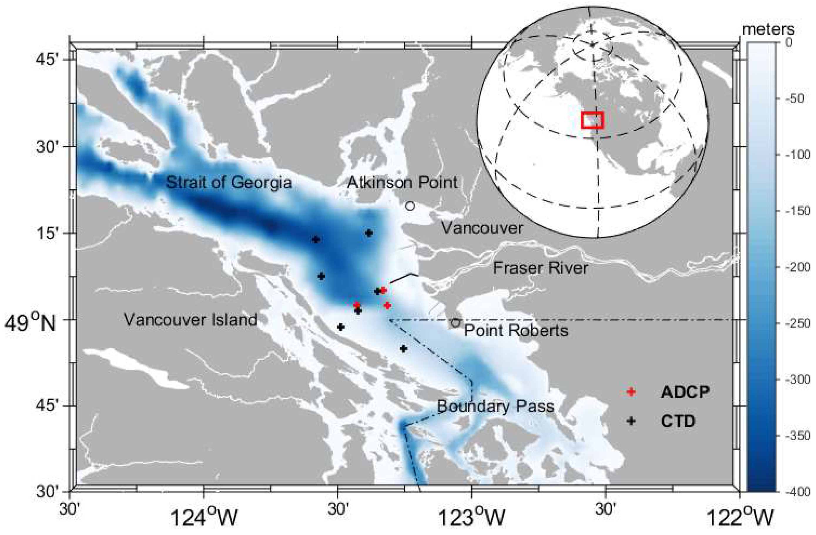
Ocean Networks Canada (ONC) placed three sets of real-time observation bottom nodes in the Strait of Georgia as part of the ONC Victoria Experimental Network Under the Sea (VENUS) coastal observatory. Figure 1 shows the locations of these nodes, which include bottom-mounted acoustic Doppler current profilers (ADCP). Since 2008, two 150 kHz RDI Teledyne ADCPs and a 300 kHz RDI Teledyne ADCP were deployed separately at depths of 170 m, 300 m, and 100 m, respectively. More information about these observations is given by Li et al. [7].
Pawlowicz et al. from the University of British Columbia (UBC) have performed the conductivity-temperature-depth (CTD) observations on multiple sites in the Strait of Georgia for a period of more than three years from April 2002 to June 2005. The CTD profile observations were performed once or twice every month. The velocity fields from the SalishSeaCast model by Soontiens et al. [12] and Soontiens and Allen [13] were downloaded from their ERDDAP server (https://salishsea.eos.ubc.ca/erddap/) between 12:30 29 May 2018 to 12:30 30 May 2018 from datasets: ubcSSg3DuGridFields1hV17-02, ubcSSg3DvGridFields1hV17-02. From these data we can obtain the background currents in the Strait of Georgia with time resolution of about 1 h and spatial resolution of about 500 m. Weather information for wind comes from SAND HEADS (climate ID 1107010 in Environment Canada). This station is located at the end of the Fraser River’s estuary breakwater, and provides a time series of 2 min averaged wind data recorded once every hour at a height of 11 m. The general wind situation in the Strait of Georgia can be found in [2,14].
2.2. Research Methods
2.2.1. Remote Sensing Derivation of Internal Wave Parameters
Generally speaking one can choose different one-dimensional internal wave propagation models to simulate the propagation characteristics of internal waves based on the horizontal scale of the internal waves as well as its relation with the depth and the stratification of water. For example, we can choose the KdV equation [15,16] for the long internal waves in shallow water, and here it means the wave length is greater than the water depth and of course greater than both the upper and lower layer if it is a two-layer system. If the wavelength of the internal wave is close to the depth of water, the Joseph-Kubota equation can be adopted [17,18]. The Benjamin-Ono equation [15,19] can be used if the wave length of internal wave is much less than the depth of water and the stratification is contained in a thin layer for a continuously stratified system, or when wave length is greater than one layer but less than the depth of the other layer for a two layer system. In the Strait of Georgia, the average depth of water is about 150 m while the upper layer depth of water is about 2–5 m in the summer [4]. The wave amplitude (the maximum displacement) varies between 2 and 8 m [4] in the summer and can be as large as 30 m [7] in the winter and the wave length can be as large as 100 m. As a result, we consider the observed internal waves as deep water nonlinear internal waves, to which the Benjamin-Ono equation is more applicable. This was confirmed by Wang and Pawlowicz [4] by comparing their observations in the Strait of Georgia and different theories including Benjamin-Ono equation. The Benjamin-Ono equation can be written as [4,15,19]
where the nonlinear coefficient α and the dispersion coefficient β are given by
And is the mode shape solution of the Taylor-Goldstein (TG) equation [20], is the corresponding linear internal wave phase speed, is the best thickness of the upper layer for a continuously stratified system where reaches its maximum as defined in [21].
The algebraic solution of Equation (1) is
In the above equation, is the wave amplitude, and are the half-wave width and the phase speed of the internal wave, respectively, which can be expressed as
Satellite images of sea surface roughness—for example, obtained by synthetic aperture radar (SAR) or by radiometers viewing areas in and around sun glitter—at times provide clear observations of short-period internal waves (also usually termed internal solitary waves—ISWs). The surface manifestations of ISWs are characterized by enhanced and reduced roughness of the sea surface arrayed in parallel bands with scales of hundreds of meters wide and tens of kilometers long (see e.g., [1]). These bands result from the modulation of surface gravity-capillary waves due to convergent and divergent currents originated by the ISWs. Both along-wind and crosswind current gradients can produce roughness variations that exhibit surface roughness signatures in reflectance satellite images. The wind direction and the sensor look direction are irrelevant for divergence detection (see [22]). Imaging mechanisms are usually based on weak hydrodynamic interaction theory following the traditional relaxation approximation (e.g., [11,23,24]), according to which the wave action N(x, k, t) is written as:
where it is supposed to experience a small disturbance δN with respect to a background value N0 corresponding to the state undisturbed by currents. Here x is the horizontal position and k is the wavenumber, and in the presence of a variable current u, the action anomaly δN due to current variations can then be written as,
where repeated indices i, j = 1 to 2 indicate summation over horizontal components and the time scale τc(k) depends on the wavenumber k, where we assume that the typical length scale of the internal wave current variation is much larger than the relaxation length scale. It should be pointed out that the conventional radar imaging theory based on weak hydrodynamic interaction theory and Bragg scattering theory as in [1] fails to describe the often observed strong radar signatures of internal waves and their weak dependence on look direction of the radar antenna. In those cases, breaking wave modulation [25] or a process involving cascade modulation from long to intermediate and short wind waves [26] have been proposed. However, in our study region, we think those processes involving breaking wave modulation are not so important to the imaging mechanism due to the reduced wave amplitudes and phase speeds compared to the tropical oceans where these are more relevant.
Hence, as a first approximation, the remote sensing image contrasts ξ are proportional to the internal wave generated current gradients, and we write:
where x is the internal wave propagation direction.
The surface flow induced by the propagation of a Benjamin–Ono internal wave can be simplified for weakly nonlinear internal waves () as in [21]:
Substituting Equations (3) and (8) into Equation (7), the imaging expression for internal waves can be obtained as:
where A is a constant. Then the locations of the brightest and the darkest spots for a single internal wave can be determined by
The solution of the above equation is . Therefore, the bright and dark spacing D of a single internal wave satisfies the condition . Once the stratification and the half wave width of an internal wave are known, one can calculate parameters α and β using Equation (2) and then solve for the amplitude of this internal wave, which can then be used to solve for the phase velocity by Equation (4).
In order to obtain the half wave width of internal waves, we can first perform empirical mode decomposition (EMD) on remote sensing images. The essence of EMD method is the empirical decomposition of each internal oscillating function based on the characteristic scale of the data, from which one can obtain the intrinsic mode function (IMF), solve the signal for each layer of EMD and normalize it:
where m is the decomposition level and is the variance of the decomposed IMF. In this way we can estimate the relative energy of each layer of IMF. The signal with the maximum normalized variance is the signal representing the internal wave.
2.2.2. Extract Characteristics of Internal Waves from ADCP Data
ADCP transforms the speed signal from the beam coordinate to the Earth coordinate and the algorithm of this transformation is based on the assumption that the horizontal flow rate is uniform for each beam. However, this assumption may be interfered by internal waves. The standard algorithm combines the measured velocity of the wave at different phases to yield a horizontal velocity which is different from the actual velocity. In our observation, ADCP is installed at the bottom of the ocean while internal waves occur in the near-surface layer. The horizontal scale of the observed internal waves could be comparable to the distance between different beams. The algorithm developed by Scotti et al. [27] is adopted here. The propagation speeds and directions of internal waves are obtained by calculating the maximum value of the cross-covariance of the echo intensity between different beams by making use of the time delay of internal waves passing each beam.
2.2.3. Ray Propagation of Internal Waves
We assume the formation source of internal waves to be the ray source. Here we can use the model used by C. Wang [4,28] to verify the previously obtained results. The equation is
or equivalently
We need to know the background current field in the Strait of Georgia, the observation time t1 of the wave front of the internal waves and the starting time t0 for this internal wave propagation. We investigate the internal wave propagation based on the simple processes of ray propagation. In other words, these rays will form in a fan-shaped pattern at a specific time and location (). Then the propagation of internal waves can be simulated based on Equation(13). The simulation result will be compared with the observed internal wave captured at time t1 in remote sensing images. While in Watson and Robinson [29,30] where linear horizontal 2D-refraction of internal waves in the Strait of Gibraltar were modeled and the effect of inhomogeneous stratification, depth and background flow on the shape of fronts and rays of internal waves were discussed, apparently the above method used in this work neglected the detailed variations because in this work the aim is to find the location of the wave front instead of its exact shape. First, we ignore the effect of topography variation on the phase velocity of internal waves. As in the Strait of Georgia, the pycnocline is generally shallower than 10 m and the water depth is deeper than 120 m, the effect of topography variation on internal waves is usually negligible at locations far from the coast [4]. In addition, we have only considered the barotropic current and neglected the effect of wind on the top layer. However, the propagation speeds of the internal waves obtained from the ADCP data already include the effect of the vertical shear.
3. Results
3.1. The Distribution of Internal Waves in Space and Time
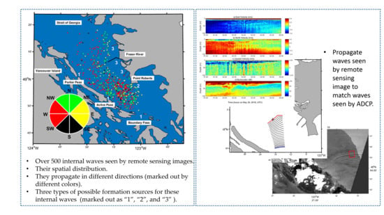
All 534 groups of internal waves, which are selected based on the previously introduced standard, are denoted on the map, as shown in Figure 2. Possible formation sources for these internal waves are divided into three categories based on their locations and propagation directions. The first category, the rough locations of which are denoted as 1 in the map, are formed due to the influence of tides on narrow channels according to Wang and Pawlowicz [6]. This type corresponds to most of the eastward and northward waves. For example, as in Figure 3, an ERS-1 satellite images taken on 15 May 1992 at 19:04, the two wave packets in the south of the strait propagating to the north are generated at the Boundary Pass to the south of the strait. The second category, which is denoted as 2 in the map, is mostly due to the interaction between tides and topography at Point Roberts or the reflection of the northward propagating internal waves near the Point Roberts. This type is related to the presence of substantial westward waves to the west of Point Roberts, for instance the three packets of westward propagating waves to the west of Point Roberts in Figure 3. The last category, with sources denoted as 3 in the map, may be related with the generation mechanism proposed by Nash and Moum [31] who explained the formation of internal waves due to river plume interactions. This type explains most of the westward propagating internal waves near the river mouth of the Fraser River, such as the wave packet propagating towards the southwest corner of the image in Figure 3.
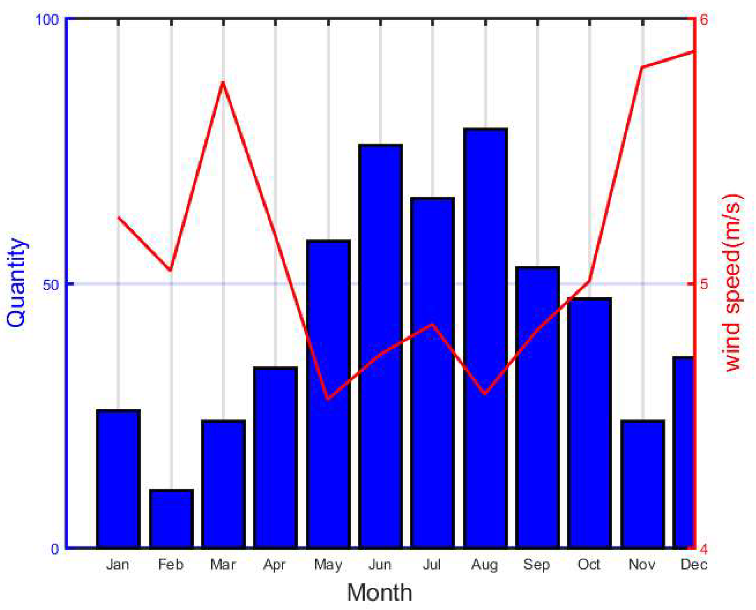
In this work, more internal waves are captured in satellite remote sensing images in the south of the strait, which indicates higher occurrence frequencies for the first and second types of internal waves than the third type. We performed statistical analysis of internal waves by month. As shown in Figure 4, it is apparent that the amount of internal waves is higher in summer compared to other seasons. This is very different from Li et al.’s [7] statistical analysis based on ADCP data, from which they concluded that the occurrence frequency of internal waves is not very different between different seasons. Brandt et al. [32] pointed out that the signal of internal waves in remote sensing images is strongly related to wind speeds, with a better chance of detecting internal waves when the wind speed is low. When the wind speed is larger than 5 m/s, the image contrast for internal waves within the C band is less than 20%, which is difficult to capture visually. Silva et al. [33] also reached a similar conclusion. Figure 4 shows that the average wind speed during summer is about 4–5 m/s, while the average wind speeds in other seasons are higher than 5 m/s, which favors a higher probability for observing internal waves in remote sensing images during summer. Therefore, seasonal variation of the number of internal waves shown in remote sensing images may not reflect the realistic existence of internal waves. In addition, radar viewing direction, depth of pycnocline as well as density variation will also influence remote sensing imaging.
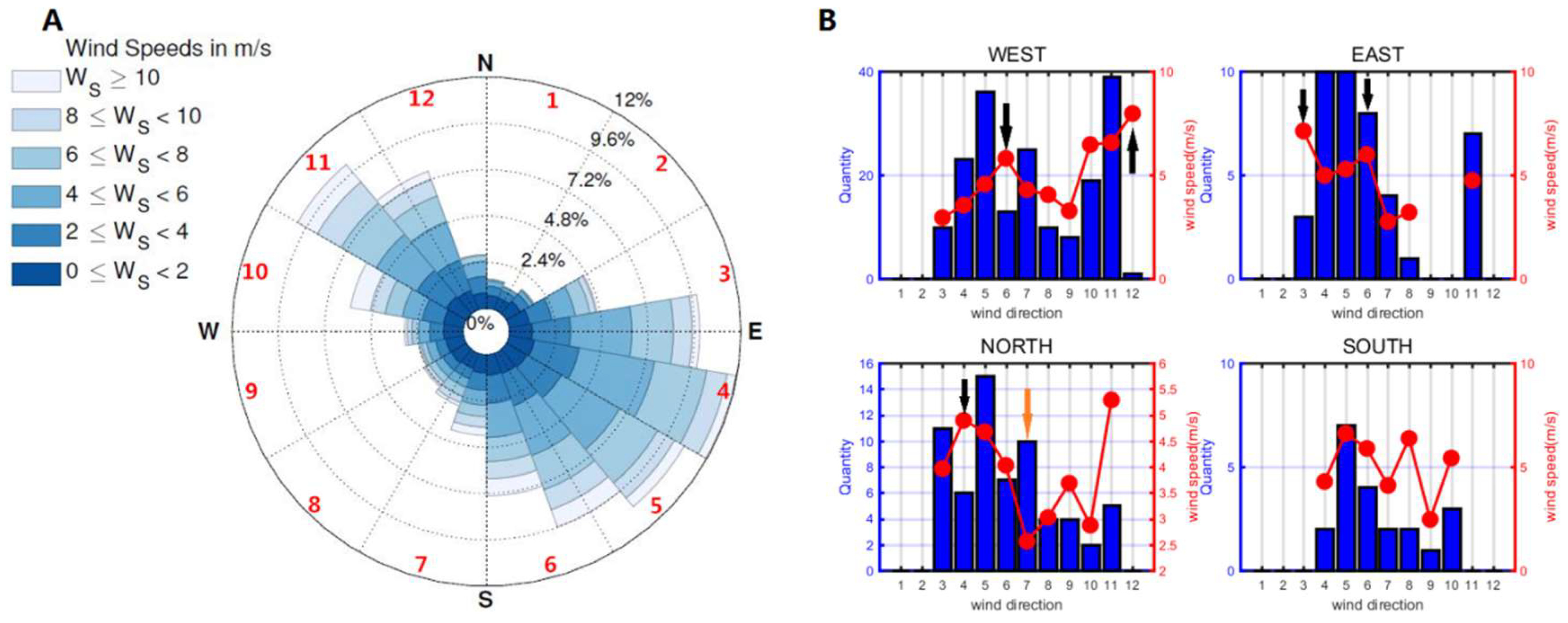
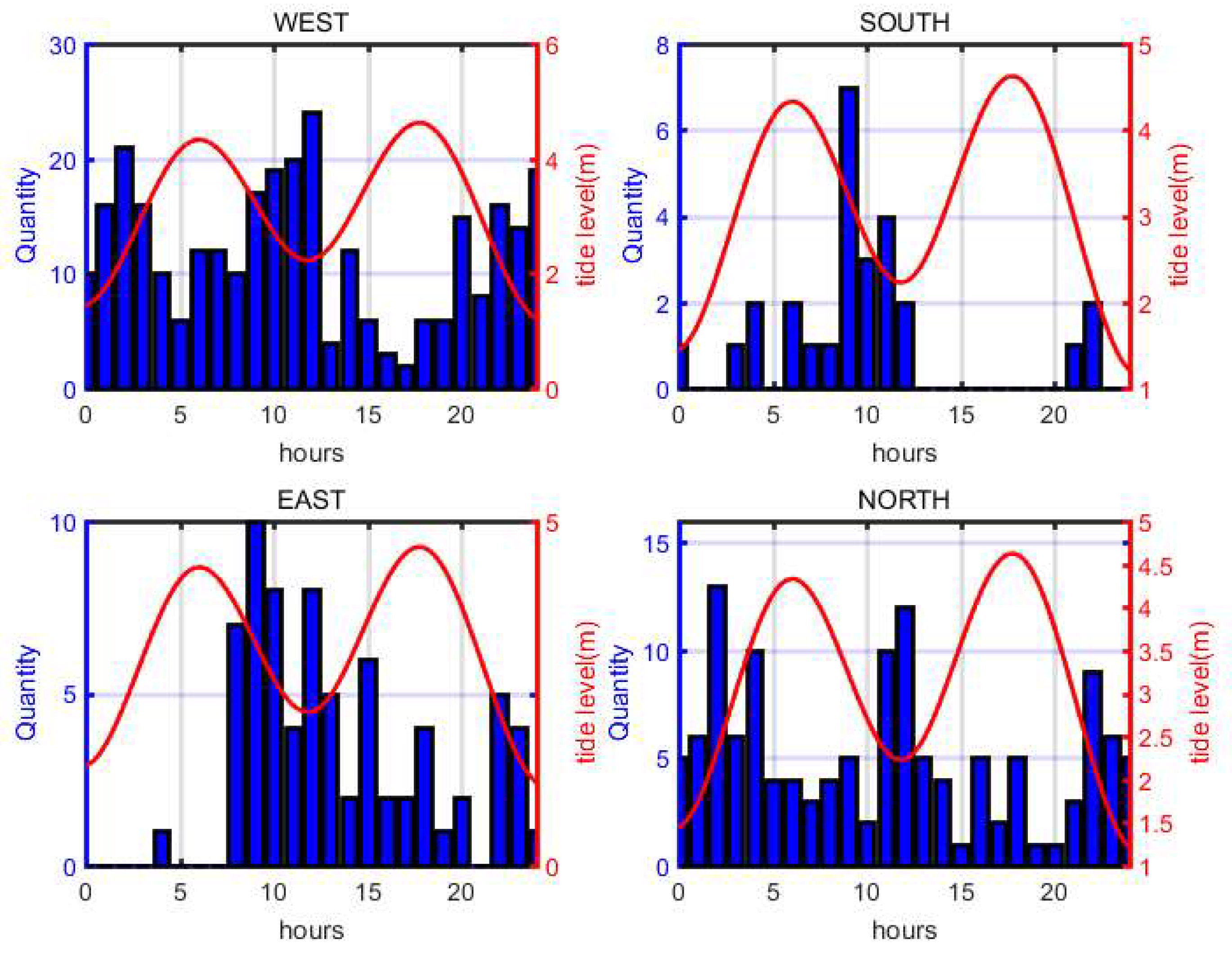
Figure 5A presents the wind rose map measured in SAND HEADS station between 2003 and 2015. It shows that the wind direction concentrates on the southeast and northwest directions, with more southeast wind than northwest wind. Most of the wind speed is less than 6 m/s. In order to further understand the relationship between internal waves shown in remote sensing images and the wind (see the red number in Figure 5A), we counted the number of internal waves in different wind directions as shown in the blue bar chart of Figure 5B. Also shown in Figure 5B by the red dotted lines is the wind speed averaged over six hours before internal waves are capture by corresponding remote sensing images. We can see that the number of internal waves decreases suddenly in directions 6 and 12 for the WEST (westward propagating) internal waves, in directions 3 and 6 for the EAST (eastward) internal waves and in direction 4 for the NORTH (northward) internal waves. Observing that in these wave and wind direction combinations the wind speeds are all higher than 5 m/s, we speculate that the increase of wind speed is the reason leading to the decrease of discernible number of internal waves in remote sensing images. The detected number of northward internal waves increases suddenly in wind direction 7. However, Figure 5A shows that the probability of wind direction 7 is not high. We notice that the wind speed in direction 7 for northward waves has decreased to 2.5 m/s. The smaller wind speed makes internal waves more easily captured by remote sensing images.
Each day the Strait of Georgia experiences two high tide levels with different heights. Similarly, each day there will be two different low tide levels with one being very low. The durations for high tides and low tides are also different. Therefore, tides in the Strait of Georgia falls into the category of irregular semidiurnal tide. We select Point Atkinson (Figure 1) in the Strait of Georgia as the reference location and calculate the time difference of internal waves being observed in corresponding satellite image relative to the preceding lower low tide. The numbers of internal waves are also counted according to the calculated time difference and the results are shown in Figure 6. It can be observed that the number of internal waves is higher during low tides than during high tides. Particularly, a large amount of eastward internal waves appear near the higher low tide, while rarely any of them is detected near the lower low tide. Such observation is speculated to relate to a higher flow velocity at the river mouth of the Fraser River during the lower low tide. Northward waves are similar to eastward waves, most of which are first-type internal waves. However, a considerable amount of northward waves come from the narrow channels to the further south of the study area. We infer that the narrow channels in the further south is less susceptible to the runoff at the river mouth of the Fraser River and therefore the tidal currents in the narrow channels can lead to the formation of internal waves in both low tidal levels. As a result, extensive northward internal waves also exist during the lower low tide.
3.2. A Case Study
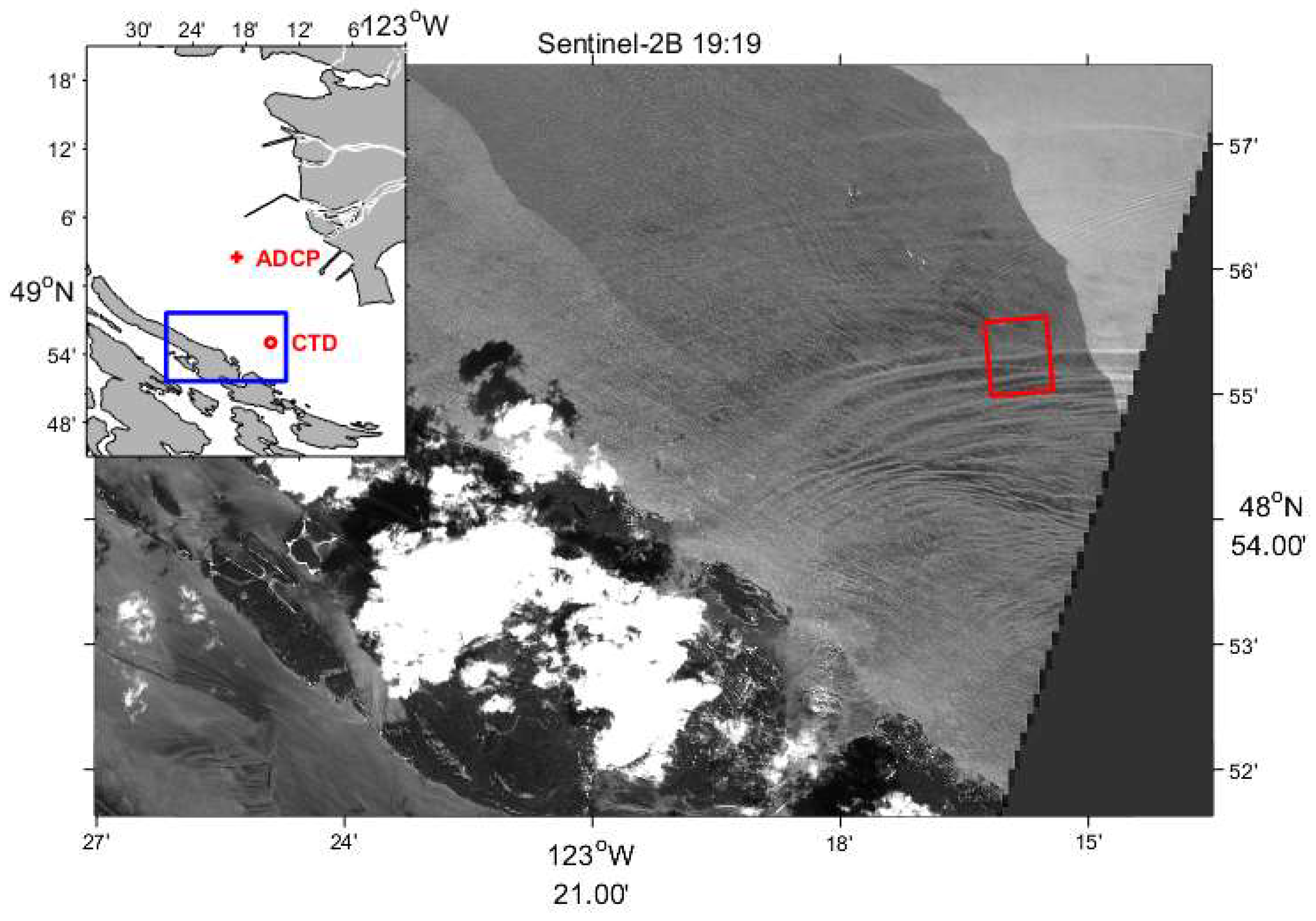
The case selected for this study is an image taken by the satellite Sentinel-2B on 29 May 2018. Figure 7 shows the B3 waveband of Sentinel-2B’s Level-1C product (central wavelength is 559 nm). Its spatial resolution is 10 m. The obvious bright and dark stripes can be observed in the image (Figure 7) and they are internal waves. The horizontal scale of its wave front is about 10 km and it propagates approximately to the north.
The ADCP data (its location is as marked out in Figure 7) on 30 May 2018 (UTC) are presented in Figure 8. Obvious signals of internal waves can be observed roughly between 02:00 and 03:30. The backscatter signal indicates that the amplitude of this internal wave is about 10 m. By applying the algorithm developed by Scotti et al. [27] as explained earlier, the propagation direction of this internal wave is calculated to be 94.9° (east being 0° and the angle is positive counterclockwise) and the phase speed of this internal wave is 0.44 m/s and the background currents are the velocity averaged over the top 15 m.
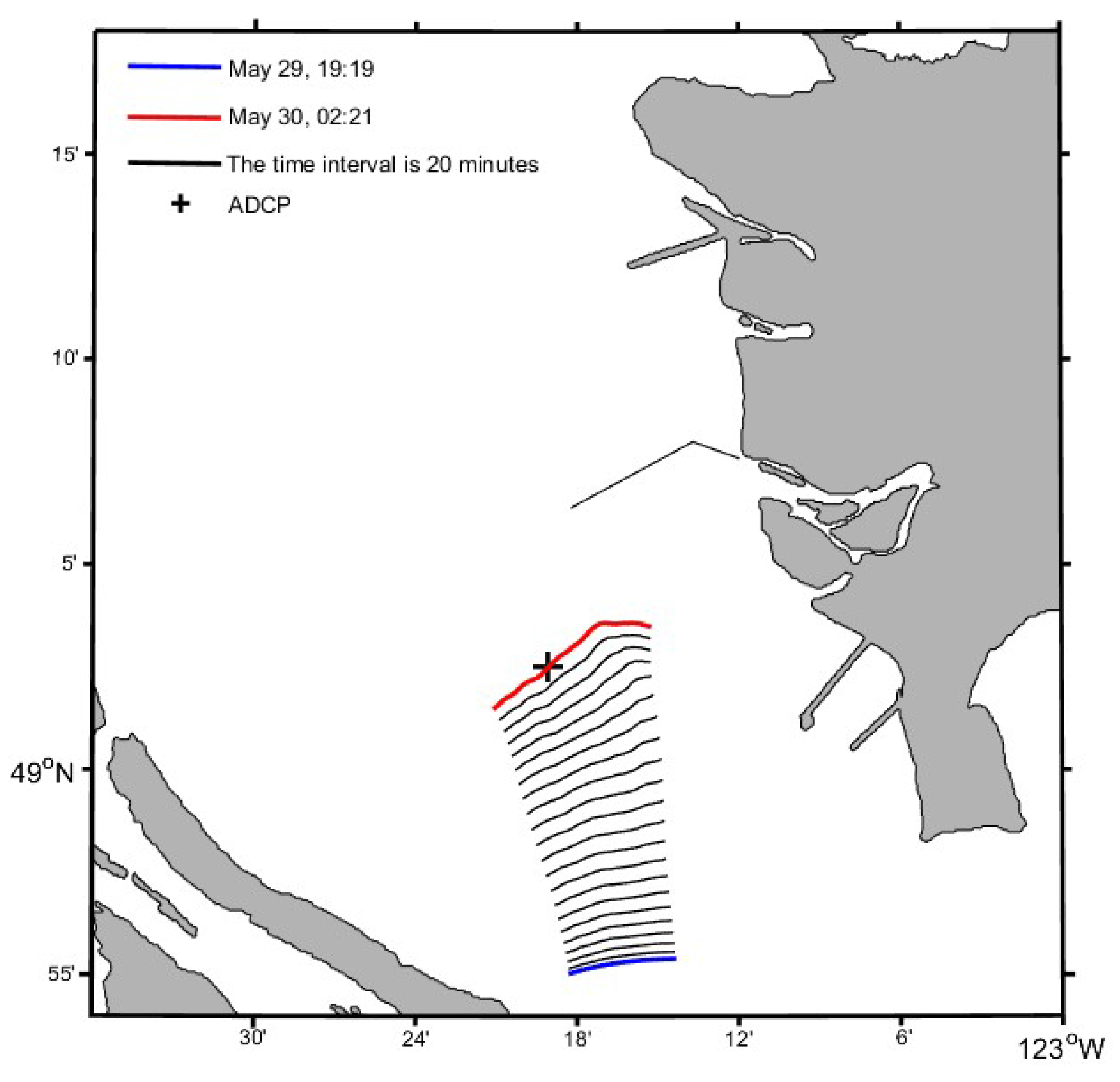
The time difference between ADCP observation of the wave and the remote sensing image (Figure 7) taken is about 7.5 h. In order to confirm the observed internal waves by ADCP (Figure 8) and by the remote sensing image (Figure 7) are the same waves, Equation (11) is used to simulate the propagation of waves along the direction of ray. The background flow field is the depth average of the NEMO model data. The phase velocity of studied wave, as mentioned earlier, is 0.44 m/s. The starting time for this propagation is the time when the waves appeared in the remote sensing image (19:19, 29 May) and the starting location is the location of the wave front in the image, as shown in Figure 9. The dark lines in Figure 9 are the simulated locations of the internal wave every 20 min. The end time of this propagation is 02:21 UTC on 30 May and the wave location is as shown by the red line in Figure 9. It is found that the simulated wave at 02:21 UTC on 30 May reached the location of the ADCP and as in Figure 8 there are large internal waves observed by the ADCP between 1:50 and 2:40. Therefore, the observed internal waves by the ADCP in Figure 8 and the waves observed by the remote sensing image (Figure 7) are the same waves.
The half wave width of the front internal wave in the remote sensing image taken on 29 May 2018 is obtained by using the EMD method to extract the distance between the bright and the dark edge of the wave in the remote sensing image along a line perpendicular to the wave crests. The location of the internal wave is in the red box area shown in Figure 7. The profile of image gray scale of the red box area in Figure 7 after averaging over the cross-front direction is shown in Figure 10. After applying EMD, as in the lower panel of Figure 10, the signal of mode 3 has the highest relative energy (45%) and thus represents the signal of the internal wave in the original signal. Calculation shows that the bright and dark spacing D of three waves are 28, 23, and 24 pixels, respectively, which correspond to an average value of 69.84 m. Then the average half wave width of internal waves can be obtained as l = 61 m. In this work 50% of the spatial resolution of remote sensing images is used as an estimation of error and considering the image resolution being 10 m, so that l = 61 ± 5 m.
We average the available CTD data at the location marked out in Figure 7 in May and June as the monthly-averaged average data for the study area, as shown in Figure 11A, B. The average data include 5 days, which are 9 May 2002, 5 June 2002, 28 May 2003, 7 June 2004, and 16 May 2015, respectively. Profiles for Dec–Jan and Jul–Aug are also included in Figure 11 for comparison. For this case study, the internal waves were observed on May 29 therefore the profile of May–Jun is used for related calculation and analysis. Figure 11A shows that density increases rapidly with depth in the upper about 10 m water. Below 10 m, the water density does not change much. The range of density is about 1016–1024 kg/m3 during May–Jun. According to Equation (4), and the calculated values of parameters α (−0.022) and β (−3.53) by Equation (2), the amplitude of internal waves is evaluated to be 10.4 ± 0.4 m and the phase speed is calculated to be 0.45 m/s. Wave amplitude and phase speed are also estimated using the KdV equation. The KdV equation estimated wave amplitude is 42 m and the estimated phase speed is 0.69 m/s. One can clearly see that the derived values of wave amplitude 10.4 ± 0.4 m and the phase speed 0.45m/s of the studied internal wave based on the Benjamin-Ono equation are very close to the ADCP observed values of over 10 m for amplitude and of 0.44 m/s for phase velocity. The KdV predictions are much more inaccurate than BO predictions. This indicates that in order to derive wave properties of the internal waves in the Strait of Georgia, the use of Benjamin-Ono equation is reasonable and reliable.
4. Conclusions
Based on the statistical analysis of a large number of remote sensing images, this paper shows that internal waves in the Strait of Georgia can be approximately classified into three categories according to their origin regions: the interaction between the tidal currents and the narrow channels near Boundary Pass and near the south of Vancouver Island; the interaction between the tidal currents and the topography near the Point Roberts or the reflection of the northward propagating internal waves near the Point Roberts; the excitation by the river plume near the mouth of the Fraser River. The number of internal waves detected in the remote sensing image is higher in summer than in winter due to the effect of varying wind speed in different seasons. The wind speed in summer is significantly lower than that in winter, making the imaging of internal waves more efficient in summer. Most internal waves occur around low tides, but they are subject to the influence of estuary runoff to different degrees depending on their locations. Internal waves formed in the narrow channels near the Vancouver Island occur more frequently during extreme low tides near the mouth of Fraser River, while their occurring frequencies are high in both low tides in the south of the study area. At the same time this work combines remote sensing and in situ observational data including ADCP and CTD to calculate and also use the Benjamin-Ono equation to simulate the characteristic properties of one internal wave for a case study. The result showed that the application of the Benjamin-Ono equation in order to derive the internal wave properties in the Strait of Georgia is reasonable and practical.
Author Contributions
The author contributions are as following: conceptualization, C.W.; methodology, C.W., J.d.S.; remote sensing image and on-site measurement data collecting and analysis, X.W., C.W.; writing—original draft preparation, C.W., X.W.; writing—review and editing, C.W., J.d.S.; supervision, C.W.; project administration, C.W.; funding acquisition, C.W.
Funding
This research is funded by the National Natural Science Foundation of China, grant number 41576021 and 41440038 and the Key Program of the National Natural Science Foundation of China, grant number 41330960.
Acknowledgments
We would like to acknowledge the Ocean Networks Canada (ONC) for the ADCP data and the SalishSeaCast group for their modeled data. We are grateful for Rich Pawlowicz at the University of British Columbia (UBC) for his scientific discussions, supports on data resources, and valuable opinions throughout this research. We also thank Lan Li for specific suggestions on ADCP and wind data analysis.
Conflicts of Interest
The authors declare no conflict of interest. The funders had no role in the design of the study; in the collection, analyses, or interpretation of data; in the writing of the manuscript, or in the decision to publish the results.
References
- Alpers, W. Theory of radar imaging of internal waves. Nature 1985, 314, 245–247. [Google Scholar] [CrossRef]
- Thompson, D.R.; Gasparovic, R.F. Intensity modulation in SAR images of internal waves. Nature 1981, 320, 345–348. [Google Scholar] [CrossRef]
- Shand, J.A. Internal waves in Georgia Strait. Trans. AGU 1953, 34. [Google Scholar] [CrossRef]
- Wang, C.; Pawlowicz, R. Propagation speeds of strongly nonlinear near-surface internal waves in the Strait of Georgia. J. Geophys. Res. Oceans 2011, 116. [Google Scholar] [CrossRef] [Green Version]
- Wang, C.; Pawlowicz, R. Oblique wave-wave interactions of nonlinear near-surface internal waves in the Strait of Georgia. J. Geophys. Res. Oceans 2012, 117. [Google Scholar] [CrossRef] [Green Version]
- Wang, C.; Pawlowicz, R. Internal wave generation from tidal flow exiting a constricted opening. J. Geophys. Res. Oceans 2017, 122, 110–125. [Google Scholar] [CrossRef]
- Li, L.; Pawlowicz, R.; Wang, C. Seasonal Variability and Generation Mechanisms of Nonlinear Internal Waves in the Strait of Georgia. J. Geophys. Res. Oceans 2018, 123, 5706–5726. [Google Scholar] [CrossRef]
- Pawlowicz, R.R.O.; Halverson, M. The circulation and residence time of the strait of Georgia using a simple mixing-box approach. Atmos.-Ocean 2007, 45, 173–193. [Google Scholar] [CrossRef]
- Halverson, M.; Pawlowicz, R. Tide, Wind, and River Forcing of the Surface Currents in the Fraser River Plume. Atmos.-Ocean 2016, 54, 131–152. [Google Scholar] [CrossRef]
- Turner, J.S.; Benton, E.R. Buoyancy Effects in Fluids. Phys. Today 1974, 27, 52–53. [Google Scholar] [CrossRef]
- Hughes, B. The effect of internal waves on surface wind waves 2. Theoretical analysis. J. Geophys. Res. 1978, 83, 455–465. [Google Scholar] [CrossRef]
- Soontiens, N.; Allen, S.; Latornell, D.; Le Souef, K.; Machuca, I.; Paquin, J.P.; Lu, Y.; Thompson, K.; Korabel, V. Storm surges in the Strait of Georgia simulated with a regional model. Atmos.-Ocean 2016, 54. [Google Scholar] [CrossRef]
- Soontiens, N.; Allen, S. Modelling sensitivities to mixing and advection in a sill-basin estuarine system. Ocean Model. 2017, 112, 17–32. [Google Scholar] [CrossRef]
- Pawlowicz, R.; Di Costanzo, R.; Halverson, M.; Devred, E.; Johannessen, S. Advection, Surface Area, and Sediment Load of the Fraser River Plume Under Variable Wind and River Forcing. Atmos.-Ocean 2017, 55, 293–313. [Google Scholar] [CrossRef]
- Benjamin, T.B. Internal waves of permanent form in fluids of great depth. J. Fluid Mech. 1967, 29, 559–592. [Google Scholar] [CrossRef]
- Benney, D.J. Long Non-Linear Waves in Fluid Flows. Stud. Appl. Math. 1966, 45, 52–63. [Google Scholar] [CrossRef]
- Joseph, R.I. Solitary waves in a finite depth fluid. J. Phys. A Math. Gen. 1977, 10, L225–L227. [Google Scholar] [CrossRef]
- Kubota, T.; Ko, D.R.S.; Dobbs, L.S. Weakly-Nonlinear, Long Internal Gravity Waves in Stratified Fluids of Finite Depth. J. Hydronaut. 1978, 12, 157–165. [Google Scholar] [CrossRef]
- Ono, H. Algebraic Solitary Waves in Stratified Fluids. J. Phys. Soc. Jpn. 1975, 39, 1082–1091. [Google Scholar] [CrossRef]
- Baines, P.G. Topographic Effects in Stratified Flows. Eos Trans. Am. Geophys. Union 1995, 77, 151. [Google Scholar] [CrossRef]
- Chen, G.Y.; Su, F.C.; Wang, C.M.; Liu, C.T.; Tseng, R.S. Derivation of internal solitary wave amplitude in the South China Sea deep basin from satellite images. J. Oceanogr. 2011, 67, 689–697. [Google Scholar] [CrossRef]
- Rascle, N.; Nouguier, F.; Chapron, B.; Mouche, A.; Ponte, A. Surface Roughness Changes by Finescale Current Gradients: Properties at Multiple Azimuth View Angles. J. Phys. Oceanogr. 2016, 46. [Google Scholar] [CrossRef]
- Keller, W.C.; Wright, J.W. Microwave scattering and the straining of wind-generated waves. Radio Sci. 1975, 10, 139–147. [Google Scholar] [CrossRef]
- Alpers, W.; Hennings, I. A theory of the imaging mechanism of underwater bottom topography by real and synthetic aperture radar. J. Geophys. Res. Oceans 1984, 89, 10529–10546. [Google Scholar] [CrossRef]
- Kudryavtsev, V.N.; Akimov, D.; Johannessen, J.A.; Chapron, B. On radar imaging of current features. Part 1: Model and comparison with observations. J. Geophys. Res. Oceans 2005, 110. [Google Scholar] [CrossRef]
- Plant, W.J.; Keller, W.C.; Hayes, K.; Chatham, G.; Lederer, N. Normalized radar cross section of the sea for backscatter: 2. Modulation by internal waves. J. Geophys. Res. Oceans 2010, 115. [Google Scholar] [CrossRef] [Green Version]
- Scotti, A.; Butman, B.; Beardsley, R.C.; Alexander, P.S.; Anderson, S. A Modified Beam-to-Earth Transformation to Measure Short-Wavelength Internal Waves with an Acoustic Doppler Current Profiler. J. Atmos. Ocean. Technol. 2005, 22, 583–591. [Google Scholar] [CrossRef] [Green Version]
- Wang, C. Geophysical Observations of Nonlinear Internal Solitary-like Waves in the Strait of Georgia. Ph.D. Thesis, University of British Columbia, Vancouver, BC, Canada, 2009; p. 171. [Google Scholar]
- Watson, G.; Robinson, S. A study of internal wave propagation in the Strait of Gibraltar using shore-based marine radar images. J. Phys. Oceanogr. 1990, 20, 22. [Google Scholar] [CrossRef]
- Watson, G.; Robinson, S. A numerical model of internal wave refraction in the Strait of Gibraltar. J. Phys. Oceanogr. 1991, 21, 20. [Google Scholar] [CrossRef]
- Nash, J.D.; Moum, J.N. River plumes as a source of large-amplitude internal waves in the coastal ocean. Nature 2005, 437, 400–403. [Google Scholar] [CrossRef]
- Brandt, P.; Romeiser, R.; Rubino, A. On the determination of characteristics of the interior ocean dynamics from radar signatures of internal solitary waves. J. Geophys. Res. Oceans 1999, 104, 30039–30045. [Google Scholar] [CrossRef] [Green Version]
- da Silva, J.C.B.; Ermakov, S.A.; Robinson, I.S.; Jeans, D.R.G.; Kijashko, S.V. Role of surface films in ERS SAR signatures of internal waves on the shelf: 1. Short-period internal waves. J. Geophys. Res. Oceans 1998, 103, 8009–8031. [Google Scholar] [CrossRef] [Green Version]
Figure 1.
Bottom topography map of the Strait of Georgia. The black crosses are locations of conductivity-temperature-depth (CTD) stations and the red crosses are locations of acoustic Doppler current profilers (ADCP) stations.
Figure 1.
Bottom topography map of the Strait of Georgia. The black crosses are locations of conductivity-temperature-depth (CTD) stations and the red crosses are locations of acoustic Doppler current profilers (ADCP) stations.

Figure 2.
The spatial distribution of 534 internal waves. Colors represent different directions of propagation. Three types of possible formation sources for these internal waves are marked out using white numbers “1”, “2”, and “3” in the map.
Figure 2.
The spatial distribution of 534 internal waves. Colors represent different directions of propagation. Three types of possible formation sources for these internal waves are marked out using white numbers “1”, “2”, and “3” in the map.

Figure 3.
An ERS-1 satellite image taken on 15 May 1992 at 19:04 with examples of three types of internal waves.
Figure 3.
An ERS-1 satellite image taken on 15 May 1992 at 19:04 with examples of three types of internal waves.

Figure 4.
The monthly distribution of the 534 internal waves. The blue bar chart represents the number of internal waves and the red line represents the monthly-averaged wind speed. It is shown that more internal waves are observed during summer compared to other time of the year.
Figure 4.
The monthly distribution of the 534 internal waves. The blue bar chart represents the number of internal waves and the red line represents the monthly-averaged wind speed. It is shown that more internal waves are observed during summer compared to other time of the year.

Figure 5.
(A) The wind rose map of the SAND HEADS station; (B) the relationship between the internal waves and the winds in different directions, the blue ordinate represents the number of internal waves, the red ordinate represents the average wind speed, the abscissa is the wind direction (see the red number in Figure 5A).

Figure 6.
The relationship between the internal waves and the tide levels, the abscissa is the time of the internal waves relative to the lower low tide, and the red ordinate is the tidal level.
Figure 6.
The relationship between the internal waves and the tide levels, the abscissa is the time of the internal waves relative to the lower low tide, and the red ordinate is the tidal level.

Figure 7.
Sentinel-2B satellite image taken at 19:19 (UTC) May 29 2018.

Figure 8.
The ADCP data on 30 May 2018.

Figure 9.
The simulation of the internal wave propagation from the time the waves were seen in the remote sensing image (Figure 6) to the time they were seen in the ADCP measurement (Figure 7).

Figure 10.
Extraction of the bright and the dark spacing by empirical mode decomposition (EMD).

Figure 11.
The monthly-averaged conductivity-temperature-depth (CTD) data. (A) is density profile and (B) is buoyancy frequency profile.
Figure 11.
The monthly-averaged conductivity-temperature-depth (CTD) data. (A) is density profile and (B) is buoyancy frequency profile.


Table 1.
Main parameters of the remote sensing satellites used and number of internal waves captured.
Table 1.
Main parameters of the remote sensing satellites used and number of internal waves captured.
| Satellite | ERS-1/2 (SAR) | ENVISAT-1 (SAR) | SENTINEl-1A/B (SAR) | Sentinel-2 (Optical) |
|---|---|---|---|---|
| Service time | 17 July 1991–29 January 2011 | 1 March 2002–21 April 2011 | 1A: 3 April 2014–now 1B: 26 April 2016–now | 2A: 23 June 2015–now 2B: 17 March 2017–now |
| Revisit period (day) | 35 | 35 | 12 | 5 |
| Resolution (meter) | 30 | 30 | 5×5 | 10 |
| Number of images | 189 | 156 | 164 | 46 |
| Number of internal waves | 218 | 168 | 74 | 74 |
© 2019 by the authors. Licensee MDPI, Basel, Switzerland. This article is an open access article distributed under the terms and conditions of the Creative Commons Attribution (CC BY) license (http://creativecommons.org/licenses/by/4.0/).
Share and Cite
MDPI and ACS Style
Wang, C.; Wang, X.; Da Silva, J.C.B. Studies of Internal Waves in the Strait of Georgia Based on Remote Sensing Images. Remote Sens. 2019, 11, 96. https://0-doi-org.brum.beds.ac.uk/10.3390/rs11010096
AMA Style
Wang C, Wang X, Da Silva JCB. Studies of Internal Waves in the Strait of Georgia Based on Remote Sensing Images. Remote Sensing. 2019; 11(1):96. https://0-doi-org.brum.beds.ac.uk/10.3390/rs11010096
Chicago/Turabian StyleWang, Caixia, Xin Wang, and Jose C. B. Da Silva. 2019. "Studies of Internal Waves in the Strait of Georgia Based on Remote Sensing Images" Remote Sensing 11, no. 1: 96. https://0-doi-org.brum.beds.ac.uk/10.3390/rs11010096
Note that from the first issue of 2016, this journal uses article numbers instead of page numbers. See further details here.