Forest Stand Species Mapping Using the Sentinel-2 Time Series


1
Institute of Geography and Spatial Management, Jagiellonian University, Gronostajowa 7, 30387 Kraków, Poland
2
Geography Department, Humboldt Universität zu Berlin, Unter den Linden 6, 10099 Berlin, Germany
3
Integrative Research Institute on Transformations of Human-Environment Systems (IRI THESys), Humboldt Universität zu Berlin, Unter den Linden 6, 10117 Berlin, Germany
*
Author to whom correspondence should be addressed.
Remote Sens. 2019, 11(10), 1197; https://0-doi-org.brum.beds.ac.uk/10.3390/rs11101197
Submission received: 30 March 2019
/
Revised: 10 May 2019
/
Accepted: 17 May 2019
/
Published: 20 May 2019
(This article belongs to the Special Issue Multitemporal Remote Sensing for Forestry)
Abstract
:Accurate information regarding forest tree species composition is useful for a wide range of applications, both for forest management and scientific research. Remote sensing is an efficient tool for collecting spatially explicit information on forest attributes. With the launch of the Sentinel-2 mission, new opportunities have arisen for mapping tree species owing to its spatial, spectral, and temporal resolution. The short revisit cycle (five days) is crucial in vegetation mapping because of the reflectance changes caused by phenological phases. In our study, we evaluated the utility of the Sentinel-2 time series for mapping tree species in the complex, mixed forests of the Polish Carpathian Mountains. We mapped the following nine tree species: common beech, silver birch, common hornbeam, silver fir, sycamore maple, European larch, grey alder, Scots pine, and Norway spruce. We used the Sentinel-2 time series from 2018, with 18 images included in the study. Different combinations of Sentinel-2 imagery were selected based on mean decrease accuracy (MDA) and mean decrease Gini (MDG) measures, in addition to temporal phonological pattern analysis. Tree species discrimination was performed using the Random Forest classification algorithm. Our results showed that the use of the Sentinel-2 time series instead of single date imagery significantly improved forest tree species mapping, by approximately 5–10% of overall accuracy. In particular, combining images from spring and autumn resulted in better species discrimination.
1. Introduction
Forest species mapping is crucial for forest management, monitoring of forest disturbances, habitat and biodiversity assessment, as well as carbon cycle and energy budget estimation [1,2,3]. The use of the latest remote sensing data and methods, whether passive or active, can provide useful information regarding forest stand species composition, and, in comparison to conventional field studies, requires less time and enables the study of large and inaccessible areas [2,4,5].
To date, multispectral imagery has been the most commonly used data in forest species composition mapping studies, particularly imagery from the Landsat missions [6,7,8]. However, the use of medium spatial resolution remote sensing data such as Landsat imagery is challenging, especially in heterogeneous forests, owing to the occurrence of mixed pixels [9,10,11]. Therefore, in many cases, medium or low spatial resolution data have been used mostly for mapping broad forest types [12,13], without detailed analyses of tree species composition [14,15,16].
Other remote sensing data that are used in forest species mapping are hyperspectral imagery or light detection and ranging (LiDAR) data. Hyperspectral sensors, which monitor the Earth’s surface in contiguous and narrow bands, allow the capture of the biochemical composition of vegetation [2,9]. They provide a significant level of detail; therefore, in many studies, hyperspectral data has outperformed multispectral imagery [1,4,17]. However, from a broad set of wavebands, the optimal set must be selected [18] because most bands are highly correlated [9]. Furthermore, greater computational power is required for processing hyperspectral imagery [19]. Multispectral and hyperspectral data are often combined with LiDAR data [20,21]. When combining multispectral images with LiDAR data, it is possible to achieve high accuracies (above 90%) in vegetation mapping [22]. In addition, terrestrial laser scanning is used for tree species classification and provides very detailed information about forest structure [23]. Although LiDAR and hyperspectral data possess high potential for species classification, their operational use is restricted owing to limited availability and high acquisition costs [3,24], and the applicability of these data in a regional or global scale is still limited [25]. Therefore, optical multispectral data are often considered a good alternative to LiDAR data [26]. Currently, radar (synthetic aperture radar) data are used in tree species mapping, particularly for the determination of broad-leaved forest types [2]. Considering a variety of spatial resolutions of imagery used in the classification process, forest species composition can be mapped at several scales. With the use of very high-resolution imagery, it is possible to separate individual trees or even leaves [27]. However, when using very high spatial resolution imagery, the spectral responses of individual trees are affected by differences in canopy illumination and background signal [28]. Therefore, in vegetation studies covering large geographical areas, relatively dense and freely available multispectral imagery such as Sentinel-2 appears to be the best solution [10], and new approaches are required.
In forest tree species classification studies using multispectral imagery, the key issue is the multi-temporal methodology applied [6,29]. The general assumption is that phenological variations can increase the spectral separability between tree species; variations in reflectance caused by the phenological cycle can help in the accurate mapping of forest tree species [3]. The majority of studies on the phenology of forest trees refer to leaf seasonality [30], which includes the main phenophases such as budburst, leaf unfolding, autumn coloring, and abscission [31]. For conifers, needle appearance is an indicator of the beginning of growth; however, there is no obvious phenological phase during autumn [32]. On the contrary, seasonal variations in photosynthetic efficiency in deciduous trees are the most noticeable during autumn—the process of senescence connected to the change of leaf colors [33]. However, for some species the differences are difficult to capture; for example, hornbeam and common beech are characterized by very similar phenological phases [34]. Many studies have shown that the use of multi-temporal imagery allows the achievement of higher accuracies in mapping forest species than those produced using a single image [3,9]. However, combining individual images that achieve the highest accuracies does not necessarily lead to a high accuracy of the classification with combined images, and the timing of image acquisition is more important than the image quantity [35]. One of the newest optical satellite missions, Sentinel-2, can significantly improve forest mapping [36]. The Sentinel-2 sensor, MultiSpectral Instrument (MSI), acquires data in, among others, three red-edge bands, which are very useful in providing information about vegetation, e.g., chlorophyll content [37,38]. Furthermore, the repetition cycle of Sentinel-2A and its twin satellite Sentinel-2B is five days [39]. This short repetition cycle provides an opportunity to acquire dense time series imagery. Regarding tree species classification using Sentinel-2 data, in a study by Immitzer et al. [39], one of the earliest Sentinel-2A image acquisitions from 2015 was used to classify tree species. These authors achieved a tree species classification overall accuracy (OA) of 65% and highlighted the importance of the acquisition date. They also concluded that the spatial resolution of Sentinel-2A images may be insufficient for the classification of heterogeneous forests with fragmented species distribution and recommended combining these images with high-resolution data. Karasiak et al. [40] evaluated the potential of 11 Sentinel-2A images for the classification of tree species in southwest France and obtained OAs of classification above 90%. They highlighted the requirement for further studies of forest tree species mapping with the use of Sentinel-2 data and the assessment of imagery contribution from certain dates. Persson et al. [41] used four Sentinel-2 images to classify five forest tree species. They remarked that there is a requirement to undertake further studies of more dense time series of Sentinel-2 imagery including data from spring and autumn. Furthermore, Wessel et al. [42] conducted a study confirming the potential of Sentinel-2 data for forest species analysis. Above-mentioned studies were performed on relatively small and flat areas.
Thus, the main aim of the present study was to evaluate the performance of dense Sentinel-2 time series from spring, summer, and autumn in forest tree species mapping in a more challenging environment, i.e., mountainous area. We assessed which Sentinel-2 time series combinations were adequate for performing forest stand species classification with high accuracy (>90% of OA) and which image acquisition dates and Sentinel-2 bands contributed the most to the OA. In addition, we analyzed temporal phenological patterns of nine tree species occurring in the study area.
2. Materials and Methods
2.1. Study Area
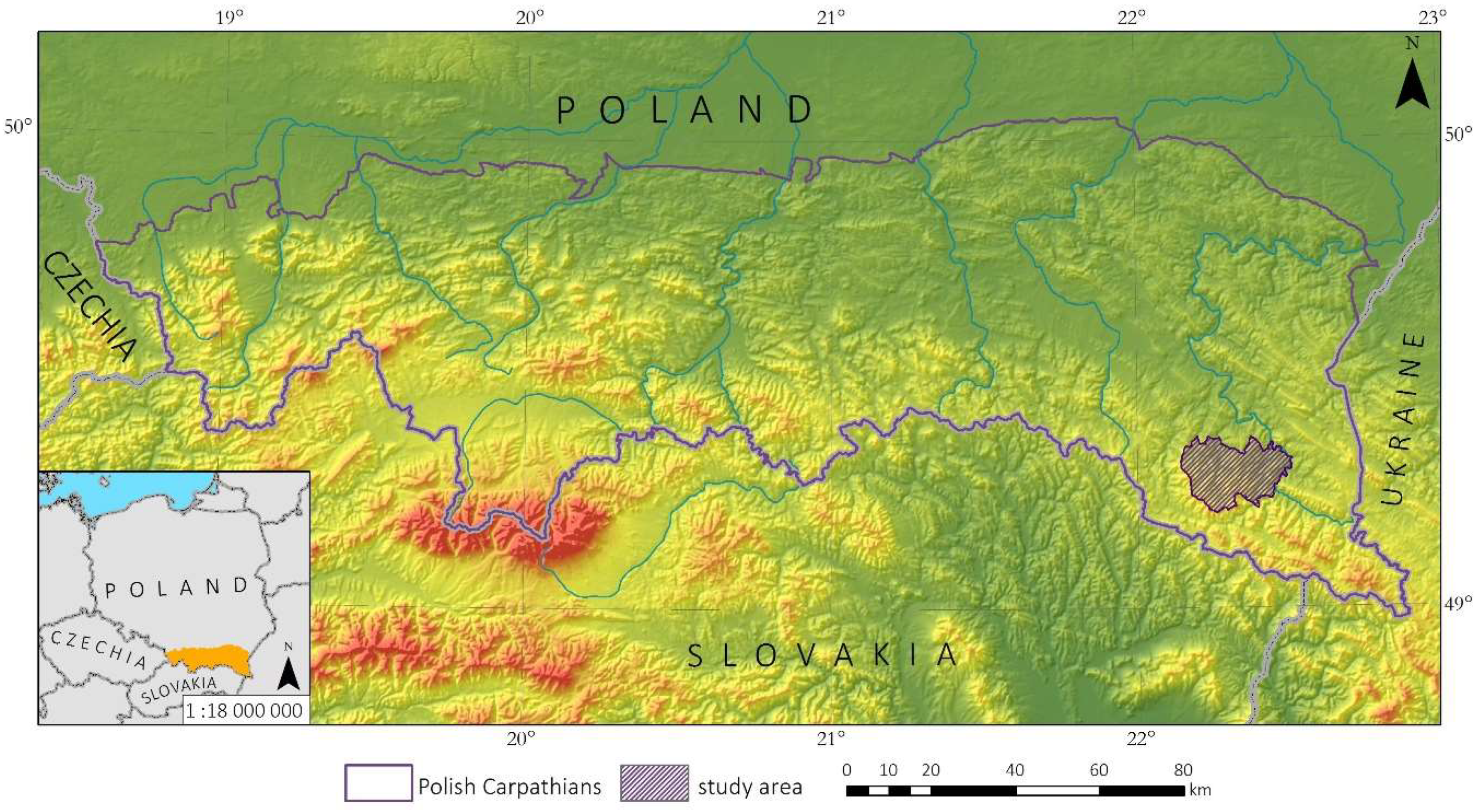
The study area is in the northern, Polish part of the Carpathian Mountains (Figure 1). Woodlands cover approximately 41% of the Polish Carpathians and are dominated by common beech (Fagus sylvatica), silver fir (Abies alba), and Norway spruce (Picea abies) [11,43]. The proportions of these three forest-forming species in the overall species composition is different in various parts of the Polish Carpathians. In the western part, the forests are dominated by Norway spruce and species diversity is low. Forests in the eastern part of the Polish Carpathians are characterized by a high percentage of common beech and silver fir [44]. Owing to the complex characteristics of tree species composition in the Polish Carpathians, the study site contained a diversified species composition, named the Baligród Forest District (Figure 1). The Baligród Forest District covers an area of 305 km2 and is in the Bieszczady Mountains in the eastern part of the Polish Carpathians. Forests here are dominated by common beech and silver fir. Other common tree species are grey alder (Alnus incana), Scots pine (Pinus sylvestris), sycamore maple (Acer pseudoplatanus), and Norway spruce. Rare species here include European larch (Larix decidua), European ash (Fraxinus excelsior), silver birch (Betula pendula), and European hornbeam (Carpinus betulus) [45]. The elevation above sea level ranges from 375 to 1070 meters a.s.l.
2.2. Data Collection and Preprocessing
In the present study, we used freely available Sentinel-2 images (Level-2A product–Bottom of Atmosphere (BOA) reflectance; tile number T34UEV) downloaded from the Copernicus Open Access Hub (https://scihub.copernicus.eu/). We used 18 topographically-corrected images distributed irregularly over the study period with no or very limited cloud cover (less than 10% of the studied forest district; Figure 2). We selected all bands with 10 and 20 m spatial resolution (Sentinel-2 bands: 2, 3, 4, 5, 6, 7, 8, 8a, 11, and 12).
Training and validation data on tree stand species composition were acquired from the Polish Forest Data Bank (Bank Danych o Lasach; https://www.bdl.lasy.gov.pl/portal/). This database is available free of charge and provides information about forest management, forest conditions and changes, detailed information on the composition of forest stands, and many other types of information [46]. The Forest Data Bank is updated every year, however, information is provided only for the Polish State Forests. The main unit here is called a subarea—homogenous forest area described and measured during inventory. A polygon represents each subarea with known coordinates. For the present study, from each subarea located in the study sites we used information regarding the share of tree species at the tree layer of the forest stand. The tree species share was estimated based on the stand volume during forest inventory. Subareas ranged in size from 0.01 to 94 ha (mean of 6.9 ha) and represent 25 different tree species. However, as described in the next section, only the most common species were distinguished in our classification.
2.3. Methods
Our workflow consists of the following steps: (1) cloud masking, (2) obtaining forest cover for 2018 (see Section 2.3.1), (3) data processing, which involved the design of training and validation samples (Section 2.3.2) and the creation of time series based on variable importance measures and temporal pattern analysis (Section 2.3.3), (4) classification of forest stand species using a Random Forest (RF) algorithm (Section 2.3.4), and (5) classification accuracy assessment of species maps for studied combinations of Sentinel-2 time series (Section 2.3.5) (Figure 3).
2.3.1. Forest Mask
First, we extracted forest areas for 2018 using Random Forest classification algorithm. The training and validation samples for this step were visually selected forested and non-forested polygons. The non-forested cover contained all non-wooded classes including built-up areas, agricultural lands, non-wooded vegetation, and water. The total number of reference areas was 27 forest polygons and 52 non-forest polygons. For this classification, one Sentinel-2 image from 20 August 2018 (the middle of the growing season and the best quality image) was used as the input data.
2.3.2. Training and Validation Samples
For the classification of tree species, all subareas from the Polish Forest Data Bank with 100% share of a particular tree species were selected. In addition, all polygons were visually checked and we removed polygons, which were not spectrally homogeneous. For less common species such as silver birch, common hornbeam, sycamore maple, European larch, grey alder, and Norway spruce, additional polygons were delineated based on subareas with 80% and 90% share of one species and visual inspection of Sentinel-2 imagery. Finally, the following nine tree species were analyzed: common beech, silver birch, European hornbeam, silver fir, sycamore maple, European larch, grey alder, Scots pine, and Norway spruce (Table 1).
2.3.3. Variable Importance and Assessment of Temporal Patterns
To select only the most important variables (acquisition dates) for classification, the evaluation was performed in two steps: the assessment of temporal phenological patterns and variable importance estimation (spectral bands and acquisition dates) using mean decrease in accuracy (MDA) and mean decrease Gini (MDG) measures. MDA and MDG are the most popular measures for variable importance embedded in RF classifier. In MDA, input variable values are randomly permuted, then the changes in predicted accuracy is measured, while MDG measures the reduction of Gini Impurity metric by a variable for a particular class [47,48,49,50]. In the majority of studies, MDA is used [47] because it is considered as more straightforward, reliable, and easier to understand [51]. However, Behnamian et al. [52] claimed that MDG is slightly more stable. Thus, we decided to use both methodologies. All statistics were calculated in R software using the randomForest package [53].
In the second step, we produced temporal phenological patterns based on ten bands from the analyzed Sentinel-2 imageries. For each band, mean spectral reflectance values for the reference polygons were extracted.
Finally, based on variable importance and temporal phenological patterns, we selected the best combinations of dates in the Sentinel-2 time series to perform further tree species classification; a total of 12 combinations and we performed classifications of all the single Sentinel-2 images separately.
2.3.4. Forest Tree Species Classification
Tree species supervised classification was performed using the non-parametric RF algorithm, which consists of an ensemble of decision trees. The main assumption behind ensemble classifiers is that when using a set of weak learners, better performance is obtained than when only a single classifier is used [54]. In comparison with other non-parametric classifiers, this algorithm is faster and less expensive computationally and, furthermore, this technique is robust with respect to overfitting and can manage many input variables without variable deletion [53,54,55]. We applied the RF algorithm in the supervised classification function from RStoolbox in R software [56]. The sample polygons described in Section 2.3.2 were used as the input reference data for classification and were randomly split into training and validation polygons in a 70:30 ratio. Then, the pixels inside the sample polygons were used to perform the classification. The number of trees was set at a default value of 500. The selected time series were clipped to only forest cover and used as the input variables during the classification procedure. The classification for each input image or combination of images was performed ten times using k-fold validation in R, and then the best one in terms of OA was selected.
2.3.5. Accuracy Assessment
We assessed the following two levels of classification accuracy: (1) maps of forest and non-forest cover (forest mask) and (2) maps of forest tree species. We visually inspected the obtained maps [57]. For the statistical accuracy assessment, the most common coefficients were calculated, i.e., OA, producer´s and user´s accuracies, and confusion matrixes [57,58].
3. Results
3.1. Variable Importance and Temporal Patterns
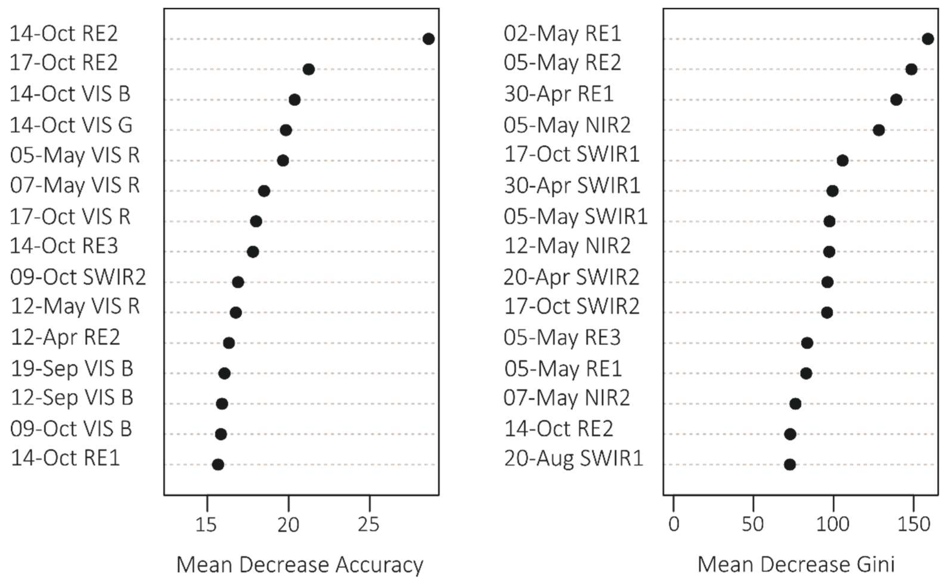
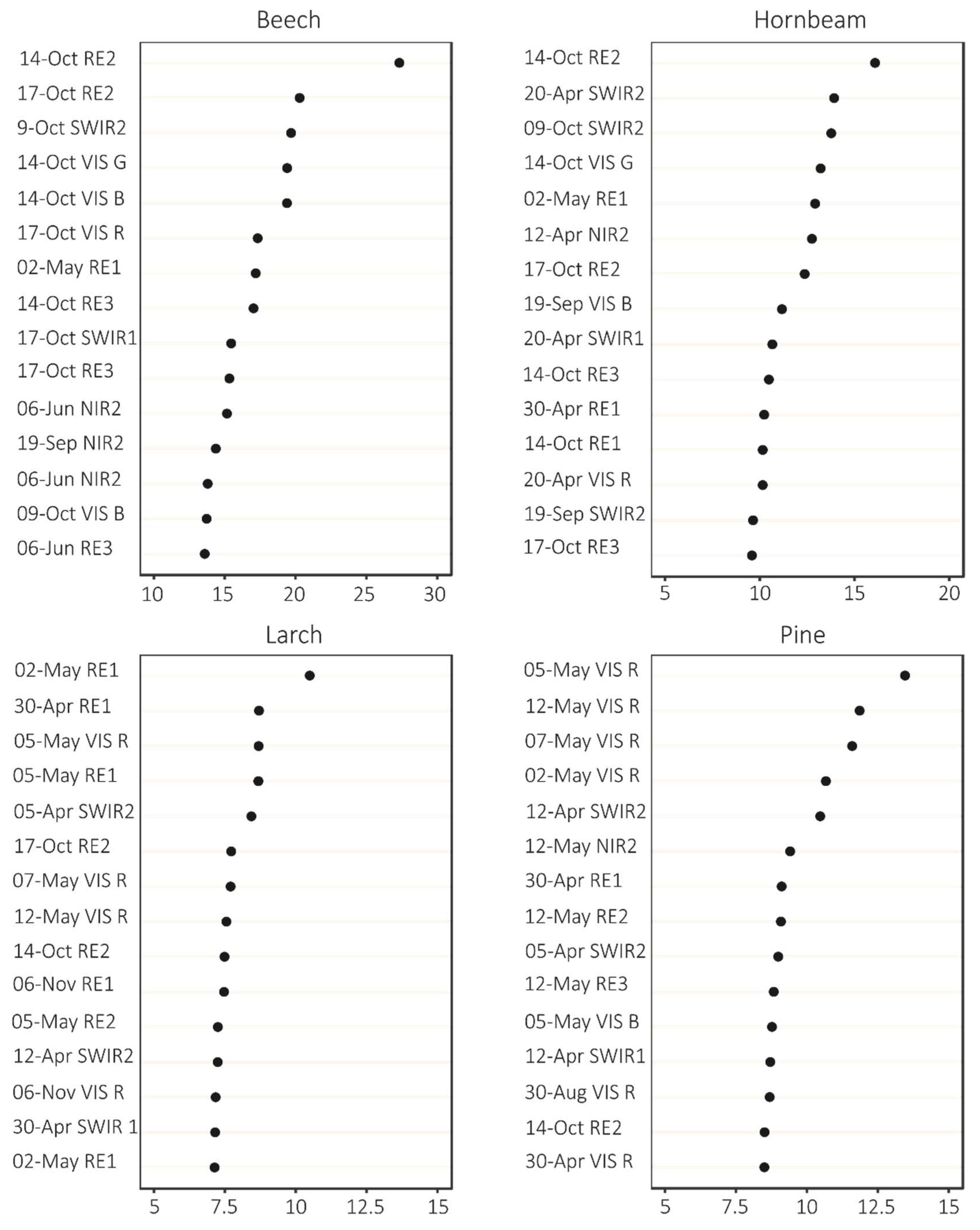
We obtained the statistics (MDA and MDG, Figure 4) for 180 bands; however, we have included only the most important ones here, i.e., 15 variables that had the highest MDA and MDG values. Based on the MDA statistics, the most significant variables included the October images (October 17 and 14), whereas MDG showed higher contribution from spring images (end of April and beginning of May). In addition, there were differences in the importance of particular Sentinel-2 bands—MDA showed the importance of visible and red-edge bands, whereas MDG showed the importance of red-edge and short-wave infrared (SWIR) bands. For the variable importance for particular forest tree species, autumn images had a greater contribution for broad-leaved species discrimination, whereas spring images showed a greater contribution for conifers (Figure 5).
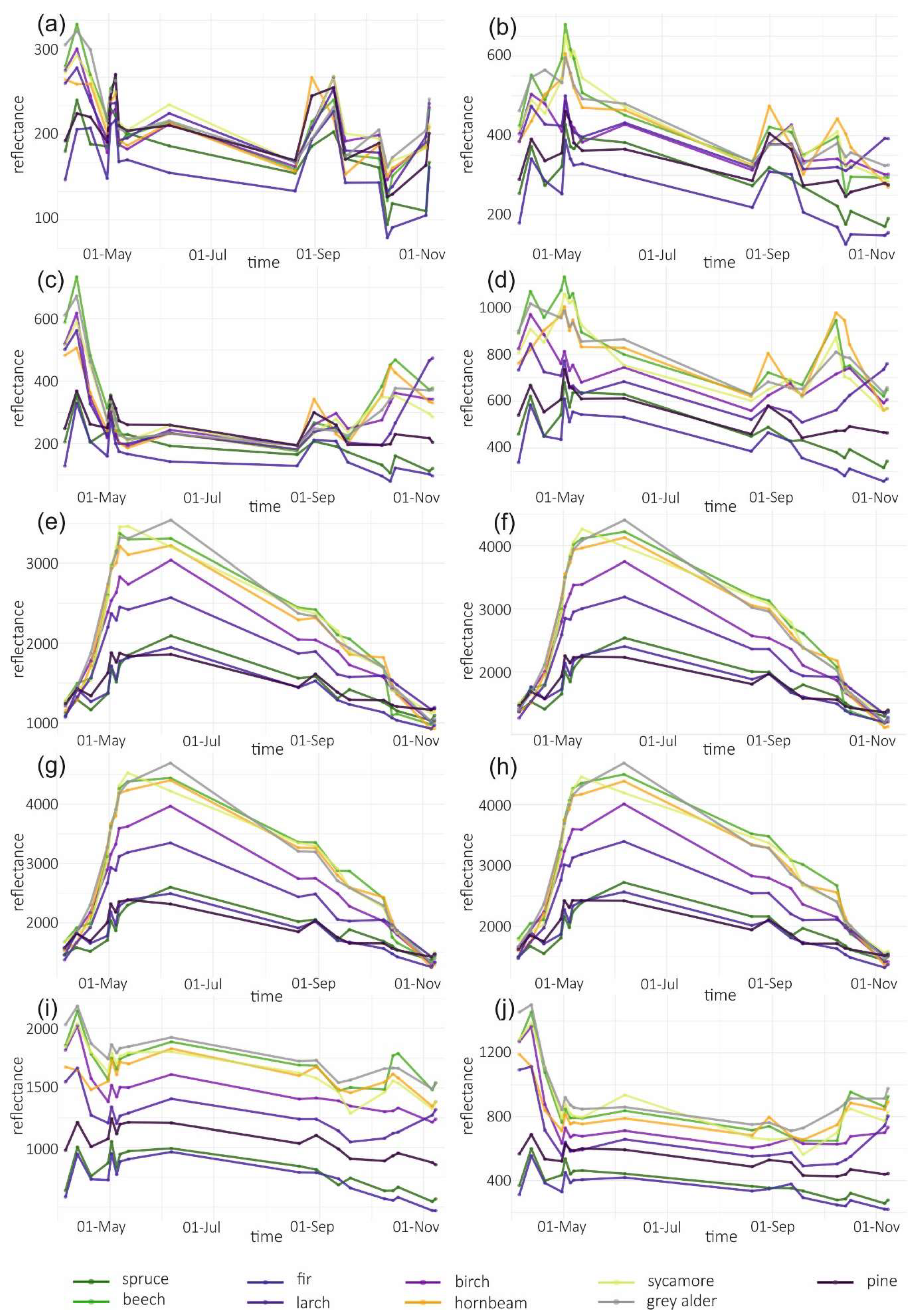
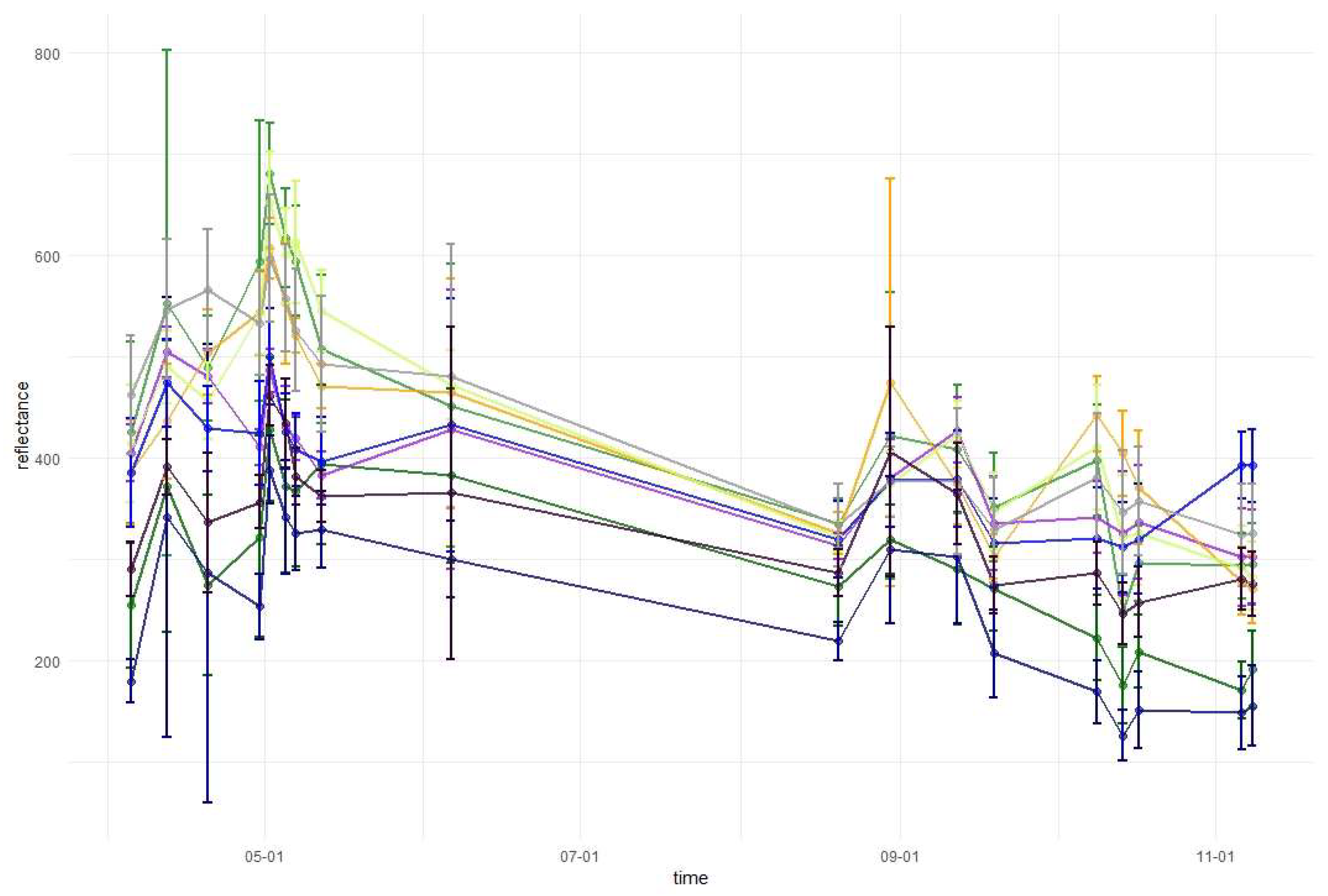
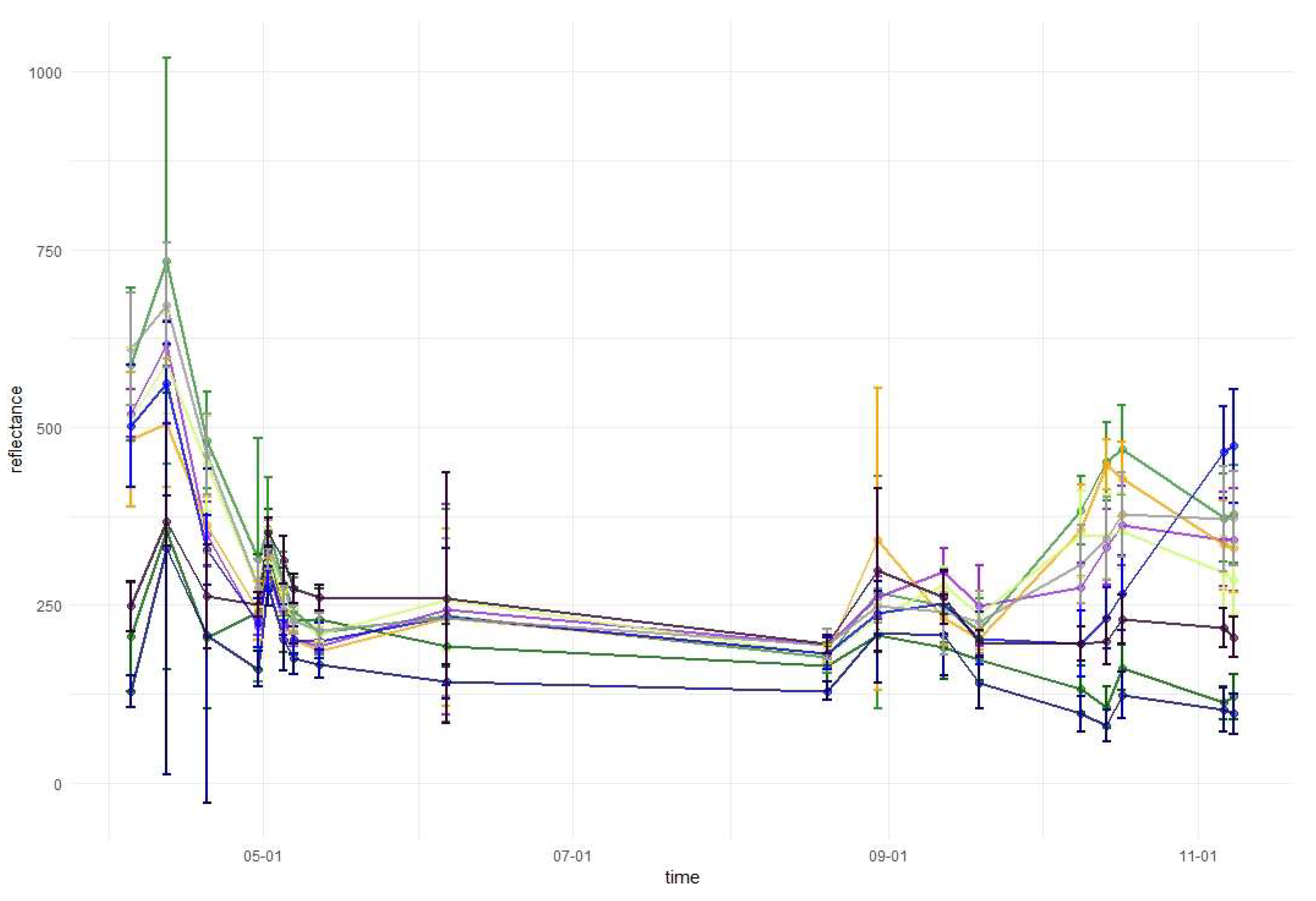
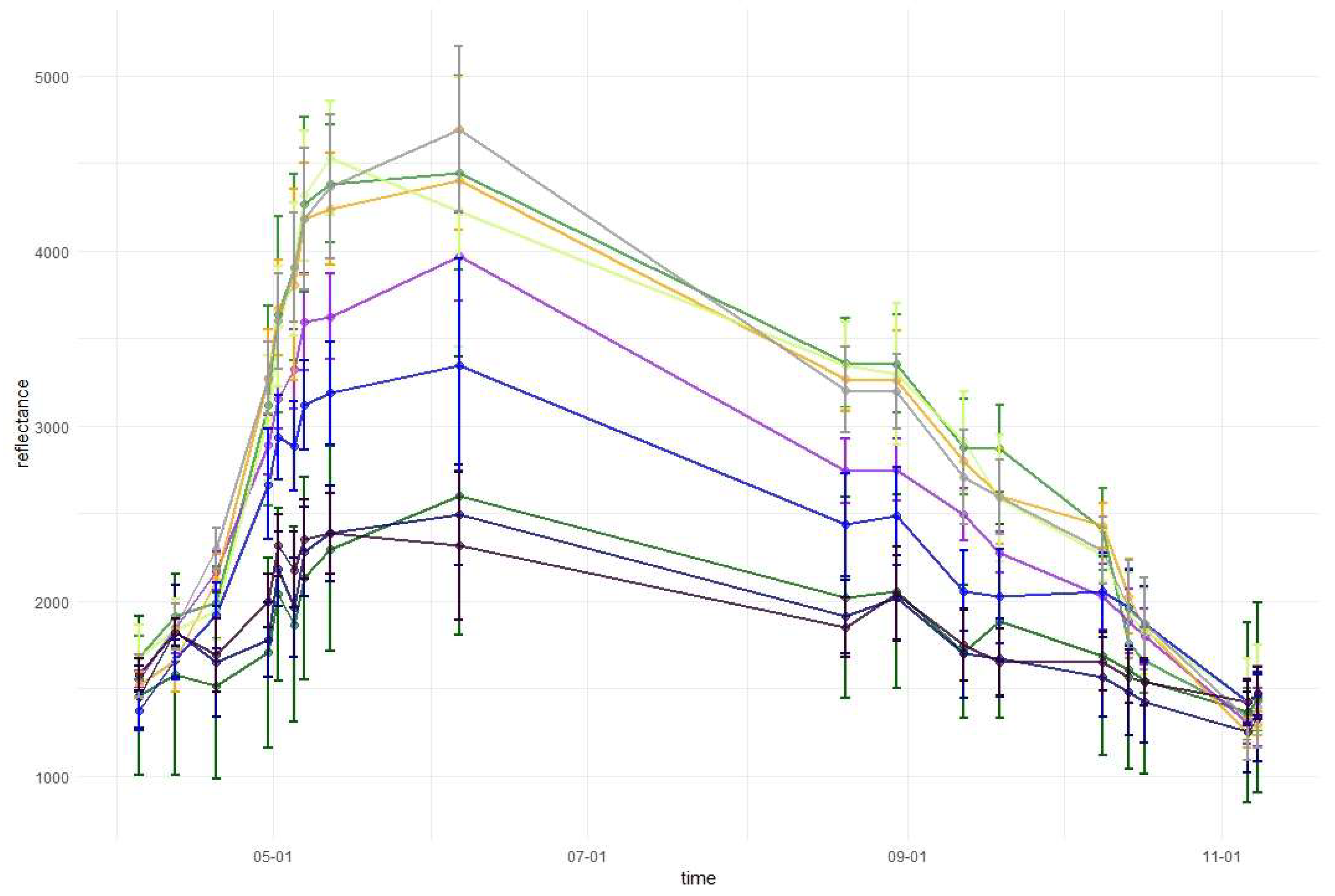
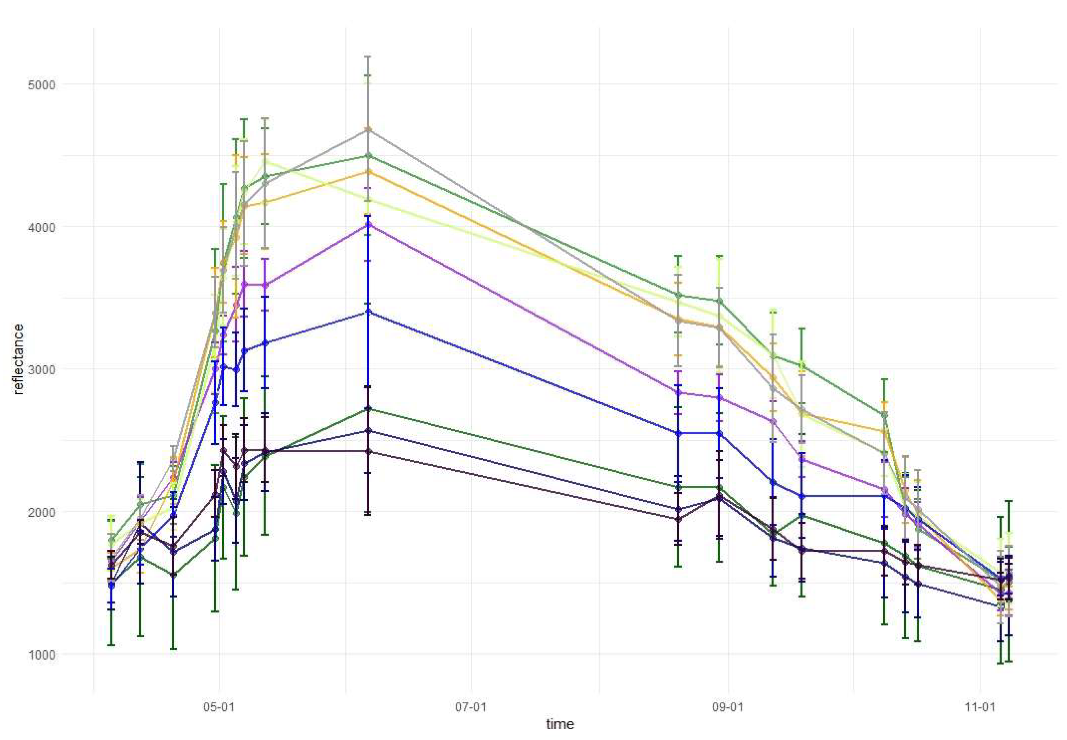
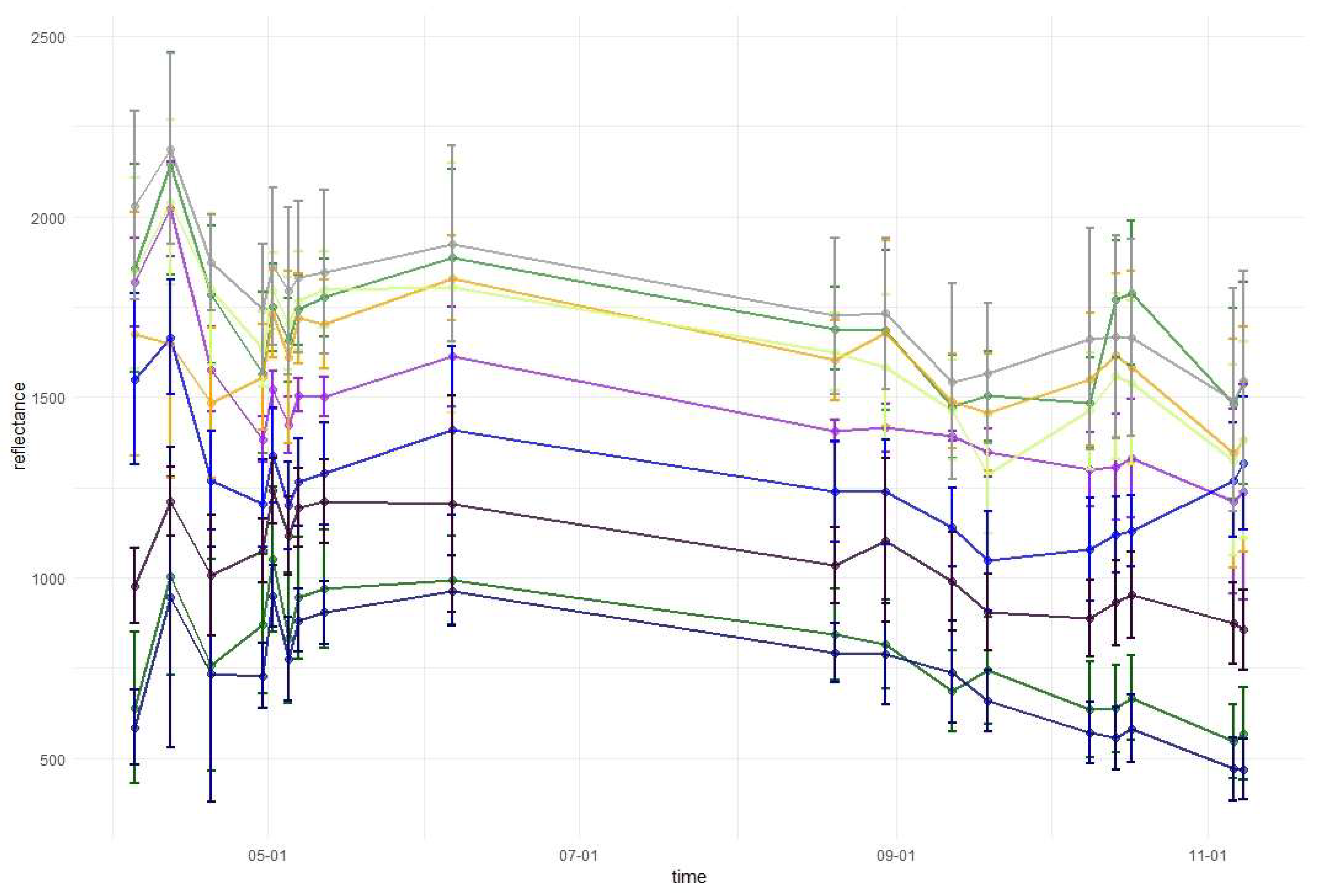
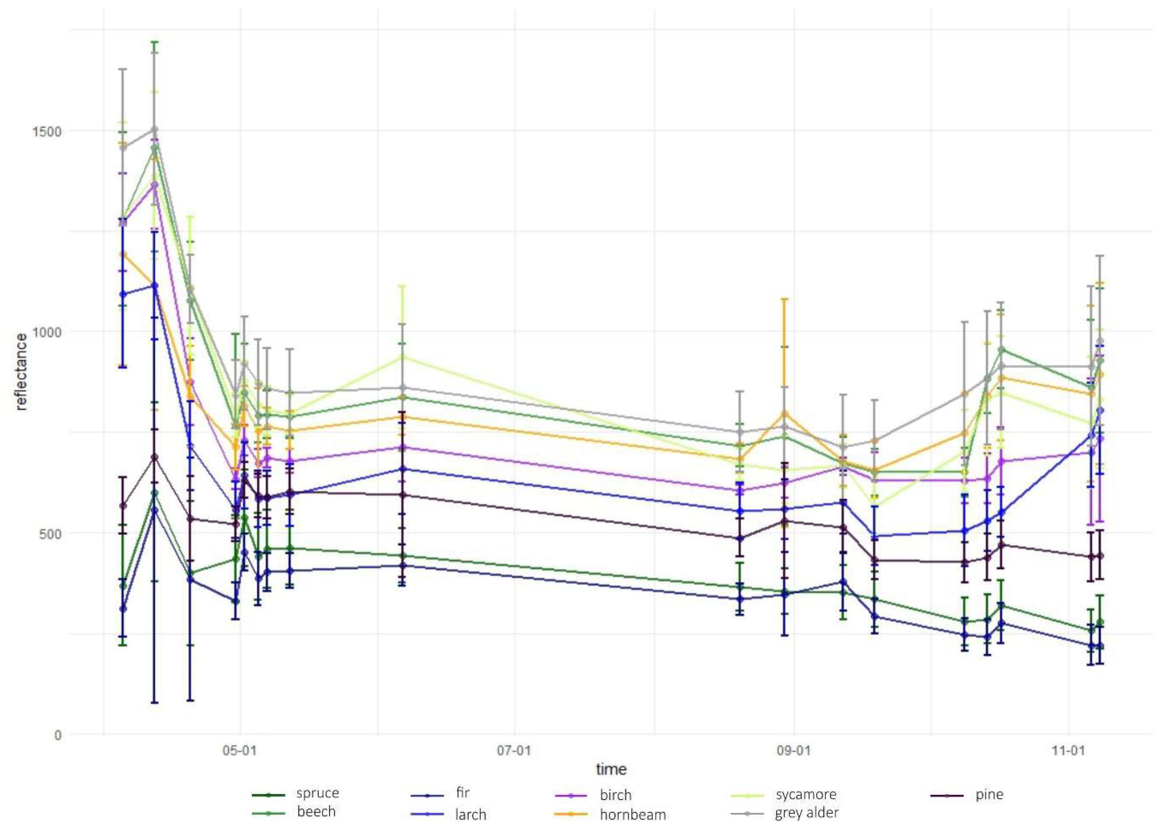
Temporal phenological patterns showed how the reflectance values varied over the 2018-growing season (Figure 6). In the visible blue part of the spectrum (VIS B, S2 Band 2), the reflectance was characterized by low and irregular values throughout the growing season for all studied species. The reflectance peaks and falls in the visible green band (VIS G, Band 3) occurred irregularly over the year, with lower values for conifers than for broad-leaved species. In the visible red band (VIS R, Band 4), the reflectance was higher during early spring and late autumn than during the middle of the vegetation cycle. Regularities occurred during autumn, i.e., from September to October there was an increase in the reflectance of broad-leaved species, a slight decrease of spruce and fir reflectance, and stable values for larch and pine. Then, in October, the trend changed for the reflectance of broad-leaved trees in VIS R, i.e., their reflectance values started to decline, whereas for larch, there was a significant increase. In general, in the visible part of the spectrum, the lowest reflectance values characterized fir and spruce. However, between May and June, pine had lower values than those for spruce. In the VIS R band, pine had higher reflectance than most of the other species during late spring and summer (May, June, and August).
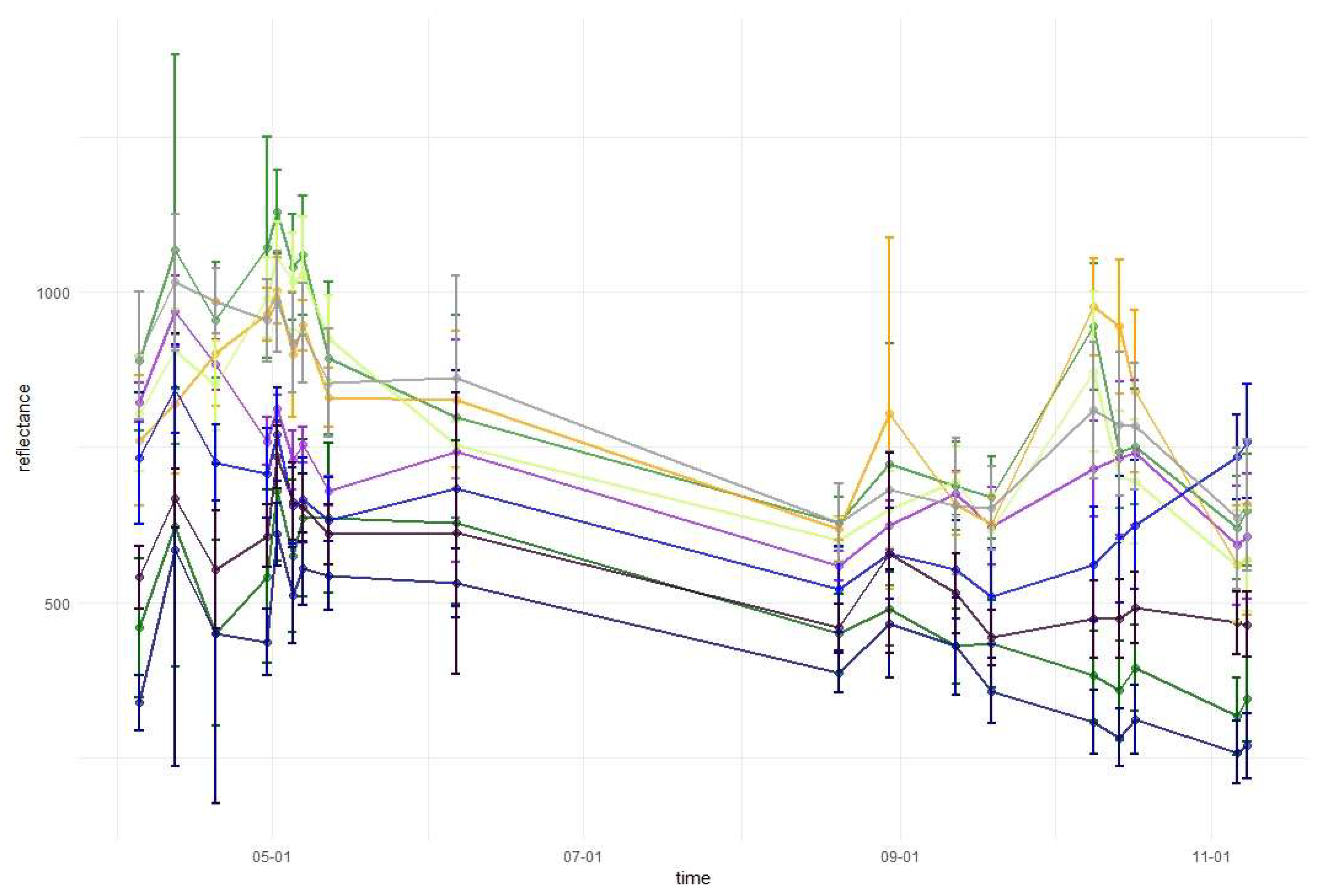
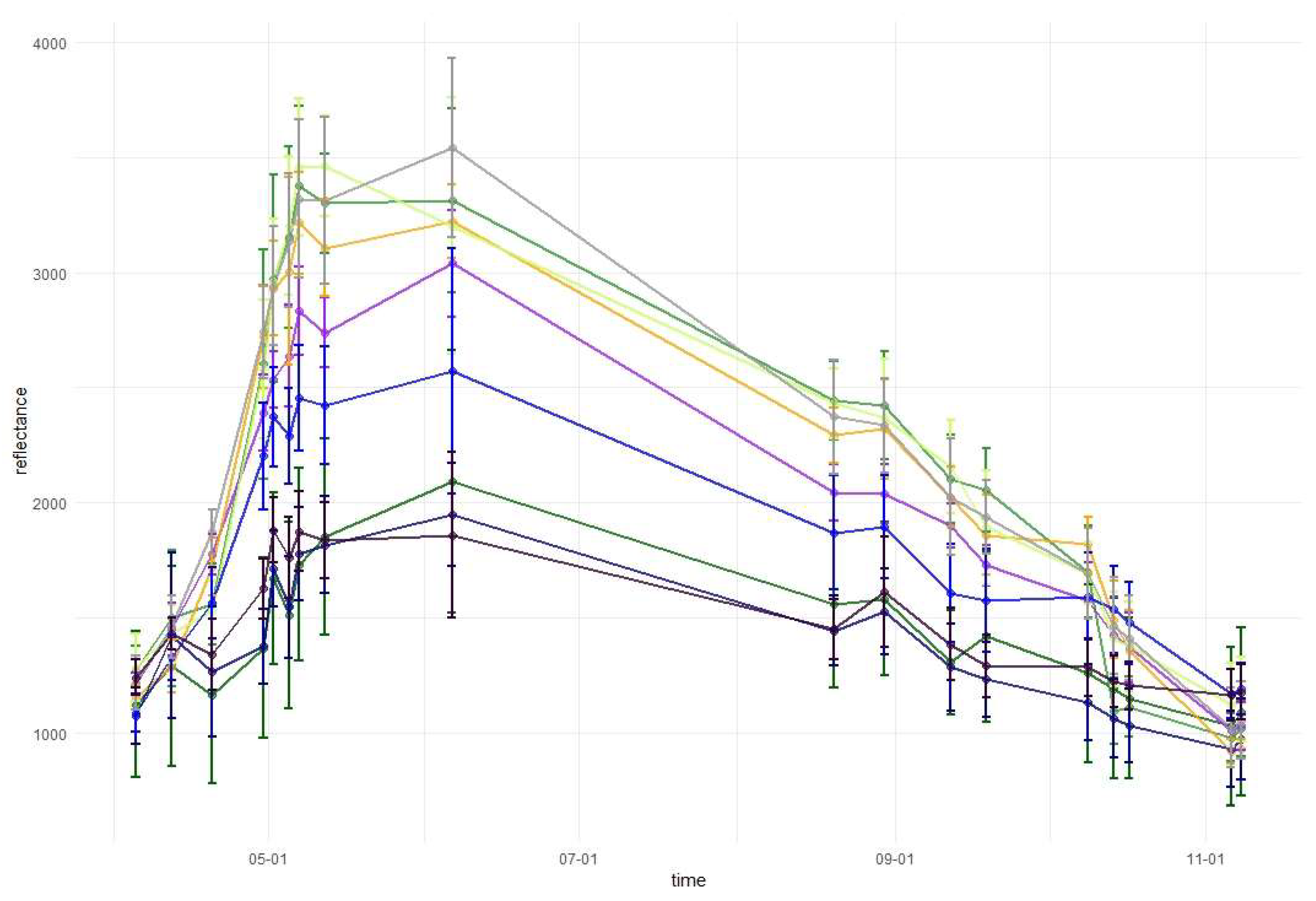
In the red-edge 1 band (RE1, Band 5) reflectance patterns are characterized by a higher diversity than in the visible bands. The reflectance for broad-leaved species was higher than conifers during almost the entire growing season. However, similarly to visible bands, during the late summer larch had higher reflectance values than that of broad-leaved species. Furthermore, larch reflectance increased during autumn in contrast to other species. Among the broad-leaved species, in the RE1 band, the highest reflectance occurred for beech (spring), grey alder (late spring), and hornbeam (late summer and autumn). Birch was characterized by the lowest reflectance. In the red-edge 2 (RE2, Band 6), red-edge 3 (RE3, Band 7), and near-infrared (NIR 1 and NIR 2, Band 8 and 8a) bands, reflectance values exhibited very similar patterns. The highest values and greatest variability between species in these parts of the spectrum occurred during late spring and summer (from May to August). The reflectance peak occurred during May (for sycamore) or June (for all other species) and after that reflectance slowly decreased. A sharp decrease in reflectance was observed for broad-leaved species between October 9 and 14. The sharpest decrease in reflectance values occurred for beech in the RE2 and RE3 bands. Among the conifers, larch spectral responses were characterized by similar properties to that of broad-leaved species. Three remaining conifer species had similar reflectance values, which were significantly lower than those of the broad-leaved values: the highest for spruce and the lowest for pine during the summer. During November, pine reflectance exceeded all the species apart from larch. Among the broad-leaved species, birch is characterized by much lower values than others.
In the shortwave-infrared spectrum (SWIR1, Band 11) the highest differences in reflectance occurred during November. For hornbeam, there was a lower reflectance during early spring than that for the other broad-leaved species; however, were similar by the beginning of May. In SWIR2 (Band 12), reflectance patterns were characterized by lower values in summer and higher values during spring and autumn. The highest peak in reflectance occurred on April 12 in both SWIR bands. Among the conifers, pine, spruce, and fir patterns were similar throughout the growing season, with similar reflectance for spruce and fir, and higher reflectance for pine. Similar to other parts of the spectrum, in both SWIR bands larch reflectance was characterized by an increase during late autumn. Based on the results of variable importance and spectral-temporal patterns assessment, we selected 12 image combinations for further forest tree species classification (Table 2).
3.2. Forest Tree Species Classification
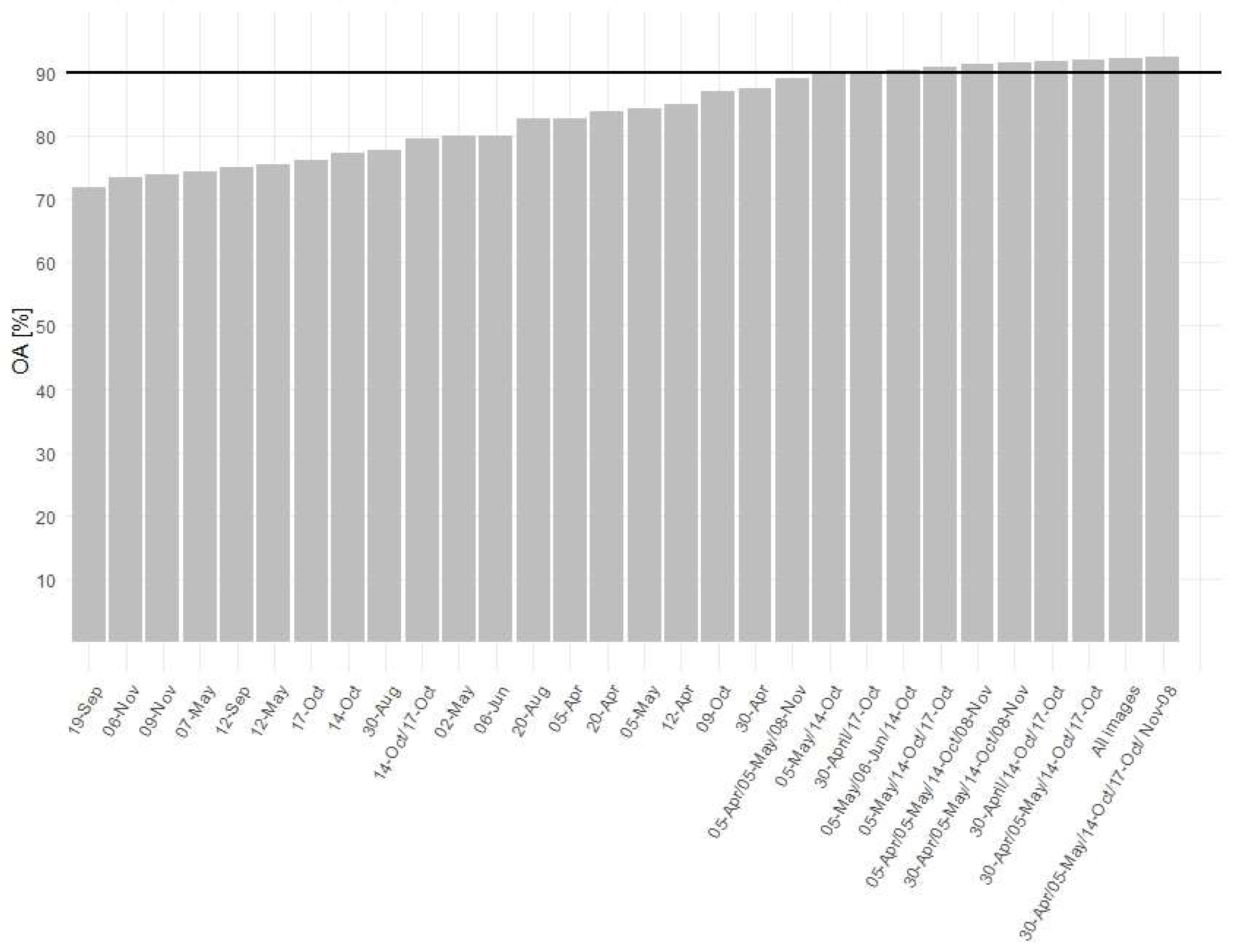
The forests in the Baligród Forest District cover 240 km2 (79% of the total area). The OA of our forest and non-forest classification was 99%. In the classification of forest tree species with single Sentinel-2 image, we achieved the best accuracy (maximum obtained OA from ten times validation) for April 30, followed by October 9 and April 12, being 87.39%, 87.08%, and 84.94% of OA, respectively (Figure 7). In the classification of the combination of two images (one from spring and one from autumn), the OA improved significantly to 90.19%. Adding more images to this combination resulted in only slight improvement; for three images (spring and two autumn images): 91.8% OA; for four images (two spring and two autumn): 92.09% of OA; and for five images: 92.38% OA. Using all available imagery did not improve forest species classification accuracy (92.12% OA).
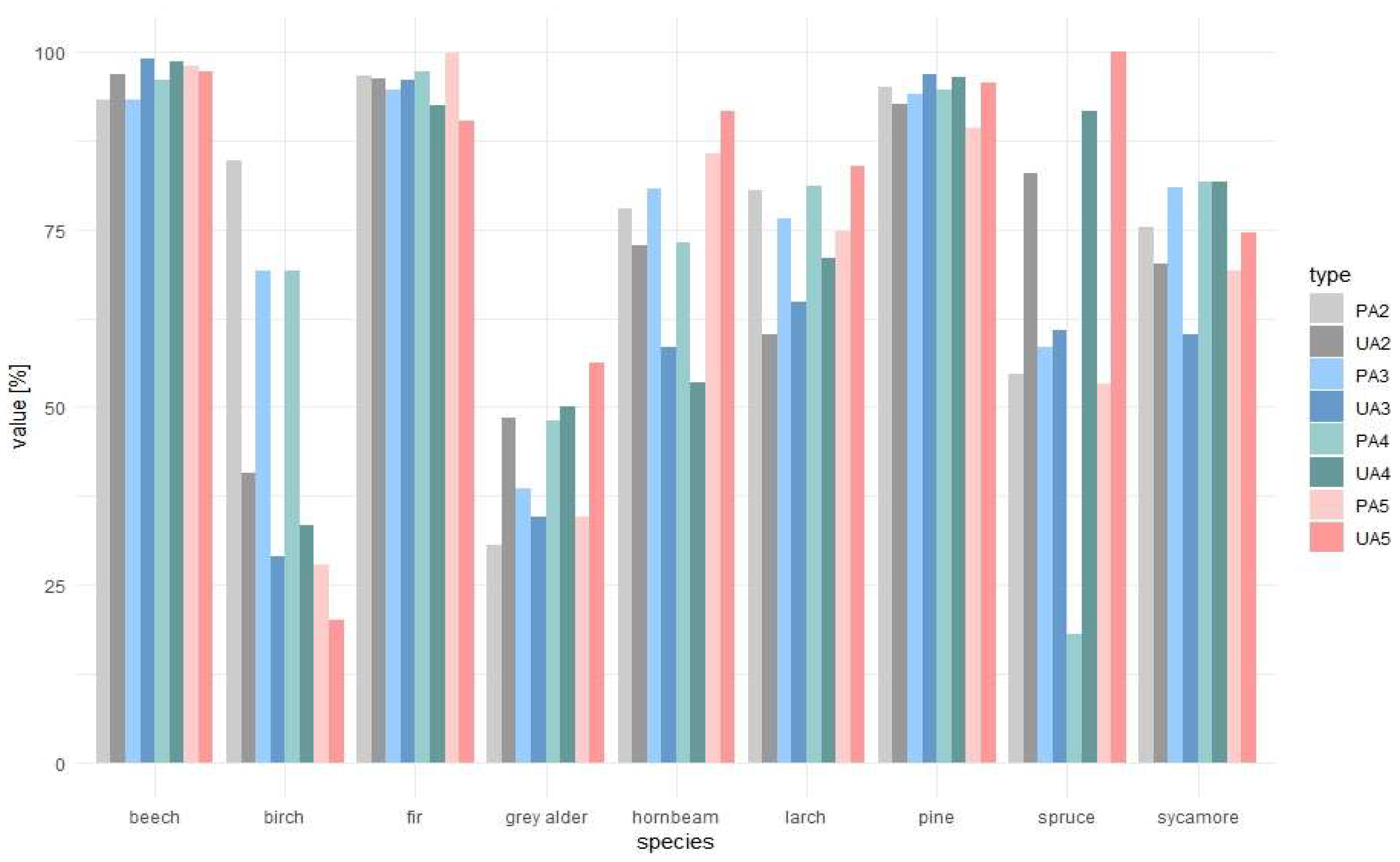
The highest producer accuracies were achieved for common beech, hornbeam, silver fir, and Scots pine, whereas the highest user accuracies for beech, hornbeam, fir, spruce, larch, and pine (Table 3). The lowest accuracies were for birch and grey alder. Combining at least two images from different seasons resulted in accurate classification (above 90%). However, using an increasing number of images for classification did not necessarily lead to higher accuracies of less common species (Figure 8). This was particularly noticeable for birch, which producers’ and users’ accuracies decreased with the increasing number of images. Accuracies for hornbeam and spruce increased and reached highest values for the classification of five images. Other species accuracies remained stable.
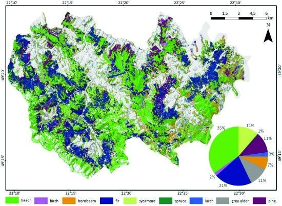
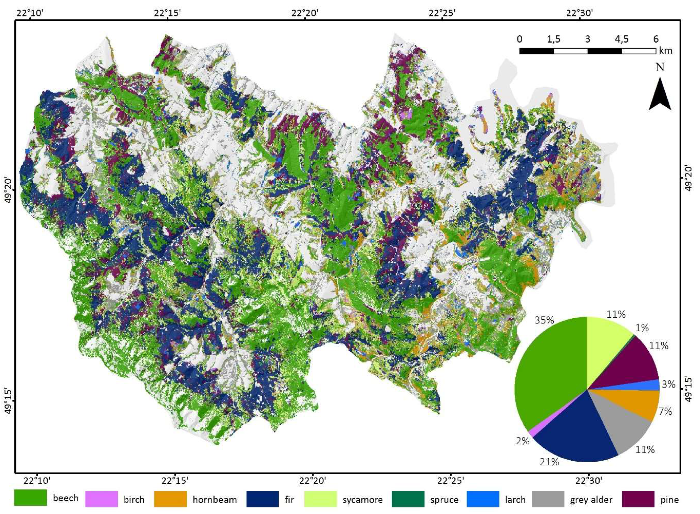
Based on classification accuracy assessment, we produced the final map of forest tree species for the best combination (April 30/May 5/October 14/October 17/November 8) (Figure 9). The most common species were common beech (35%) and silver fir (21%). Other main species were Scots pine (11%), grey alder (11%), sycamore (11%), and hornbeam (7%). The rarest species were European larch (3%), European birch (2%), and Norway spruce (1%).
4. Discussion
The present study evaluated the use of dense Sentinel-2 time series for forest tree species classification. The approach was applied in a species-diversified test site in the eastern part of the Polish Carpathians. In the study, we used dense time series from the Sentinel-2 satellite from one growing season (spring, summer, and autumn); thus, we obtained detailed information regarding the spectral–temporal patterns of the studied tree species. The outcomes from our study are similar to the results from other studies where high- or medium-resolution optical data were used [6,35,59,60]. In general, implementing multi-temporal satellite imagery improved tree species mapping accuracy. Our results show that the use of only two images from two different seasons allowed us to exceed the assumed high accuracy threshold (90% OA). However, there were some significant changes in the classification accuracy for particular tree species. Adding more variables from different acquisition dates may result in both an increase (e.g., hornbeam larch) and decrease (e.g., birch) of producer/user accuracies. Some species-specific differences are easier to capture with the use of multi-temporal imagery, while for some species using more variables may be redundant because of their high correlation. The highest contribution to the overall mapping accuracy came from spring (the turn of April and May) and autumn (mid-October) imagery. In other studies, it has been highlighted that autumn imagery tended to have a high discriminating ability [35,61,62]. In our study, the importance of two October images (14 and 17), when the leaf color changing process occurs, is indisputable. Although they were taken only three days apart, the differences in phenology proved to be crucial for the broad-leaved species discrimination, e.g., hornbeam. On the other hand, in a study by Lisein et al. [63], late spring and early summer images were optimal for discriminating of species. In addition, Persson et al. [41] found that late spring imagery performed the best tree species classification because the phenological variations are the highest during this part of the growing season. Leaf spectroscopy studies have also indicated that rapid changes in spectral values are observed during early spring and late autumn [64]. A contribution of particular imagery acquisition dates for forest tree species discrimination is different for broad-leaved and conifer species. For broad-leaved species, the most significant variables include October imagery, whereas for conifers April and May images tended to be more important. Even so, spectral signatures for some of the broad-leaved species were very similar, the greatest being for beech, hornbeam, sycamore, and grey alder. The latter species is characterized by a poor classification accuracy and adding more imagery to the classification only improved the accuracy slightly. Determining evergreen photosynthetic activity from remote sensing data is difficult; however, they also exhibit seasonal changes, especially in the visible range [65,66]. For pine, the visible part of the spectrum is significant. In general, temporal patterns for silver fir and Norway spruce are very similar, yet they differ considerably for Scots pine, indicating differences between the phenology of pines and other conifers. Finally, the only conifer but deciduous species occurring in our study area—the European larch—exhibited different properties regarding reflectance during the growing season. The spectral signatures of larch are more similar to broad-leaved species. In contrast to other species, both broad-leaved and coniferous, larch spectral reflectance increased during autumn in the visible and SWIR bands. This might result from the background signal connected to the understory vegetation in larch stands and should be examined in future studies.
In comparison to other studies on forest species with the use of Sentinel-2 data, our results (highest OA: 92.38%) are very similar to the accuracy of outcomes of the study by Karasiak et al. [40] from southwest France and higher than those from the study by Immitzer et al. [39] in Bavaria, Germany. Similar accuracies were also achieved by Puletti et al. [67] in a study area in Tuscany, Italy. However, only four broad forest types were identified there. In comparison with studies that have focused on forest species classification with the use of multi-temporal, optical imagery, the accuracies obtained in the present study were higher than those in studies where Landsat imagery was used [25,68]. Regarding similar spatial resolution imagery (e.g., 8 m Formosat-2), our results are comparable with the results of Sheeren et al. [3] even though relatively small test sites were studied. In comparison with single, very high-resolution WorldView-2 images, the multi-temporal Sentinel-2 data provided higher accuracies, e.g., the Immitzer et al. [69] study from east Austria, where the OA of forest tree species classification was 82% and the test area was much smaller (30 km2). Using IKONOS-2 imagery for Belgium, Carleer et al. [70] achieved an OA of 85.79% for tree species classification. However, Formosat-2 provides only four spectral bands (three in visible and one in near-infrared wavelengths) and IKONOS-2 also provides the same four bands plus a panchromatic band. Furthermore, WorldView-2 has lower spectral resolution (with 8 bands). From our results, it is evident that there is a benefit of using additional bands. Our results show that Senitnel-2 MSI provides valuable information on vegetation properties; the MDA and MDG statistics show that not all spectral bands contributed equally to the tree species classification. However, assessing the importance of particular dates and bands is hampered by the correlation of bands and dates. The most important bands in the present study were two SWIR bands, red-edge bands, visible blue, and visible red. The high contribution of SWIR and red-edge bands was also confirmed by Bolyn et al. [71]. The utility of SWIR regions for mapping tree species has not been fully explored yet, but the importance of these bands for tree species mapping in tropical forests was confirmed [72]. As shown in our study, the importance of these bands is high in temperate zone forests.
Regarding temporal pattern analysis, in vegetation mapping, generally, the highest reflectance values occur for the infrared region and the lowest for the visible red region [10]. In near-infrared bands, the reflectance represents radiation scattering by the canopy [38], whereas the red-edge bands are more sensitive to chlorophyll a and b levels and their variations [38,73]. In the red-edge regions, there is a sharp increase in the reflectance of vegetation [74]. From our results, this increase is more evident between RE1 and RE2 bands than that between visible light and RE1. In the SWIR region reflectance, the water absorption features are important [2,64]. For example, SWIR bands are used as key indicators in forest recovery studies [51].
The important problem in forest species mapping is the character of study sites, i.e., environmental conditions (e.g., relief or climate) or forest types and species diversity (e.g., forest management or legacies). Common problems with the study of mountainous areas are cloud cover and atmospheric and topographical effects, thus the acquisition of high-quality and cloudless imagery for key phenological periods still may be difficult [12,25]. However, this might be overcome by the short revisit time of the twin Sentinel-2 satellites. In addition, the heterogeneous stand structure or high fragmentation implies difficulties with collecting enough samples, especially for the less common and non-dominant species [39,75]. Thus, often more common species are classified with higher accuracy [25]. It has been proven that small classes tend to be misclassified [3,76]. In our study, species with the lowest accuracies were birch and grey alder, which could be explained by the small sample size as well as the forest stand properties (spectral similarity to other species and not forming homogeneous stands).
In future research, especially when larger test areas are studied, the use of additional environmental variables should be considered, as these data can help to obtain higher species prediction accuracies [77]. The phenology of species can differ across communities and can increase the overlap between species [78]. It is not only species composition that has an influence on spectral reflectance. There are also within-species variations in reflectance caused by tree age, stress, and local site conditions; openness of trees; shadowing effects; and crown health [79]. The presence of insects or diseases also has a significant effect on forest stand reflectance values and differences in growth conditions such as elevation and aspect, and soils have an influence on spectral variability within the same tree species [80]. These aspects might still hamper tree species classification studies. Thus, for larger mountainous areas, phenological patterns may be examined, e.g., for different elevation zones and aspects. However, the approach proposed in the present study demonstrates the potential of dense Sentinel-2 time series to conduct forest tree species mapping in challenging, mountainous areas. In future studies, using these dense time series will provide a valuable indicator of changing plant phenology caused by climate change. Furthermore, the data and methods used can be a great source of information for enhancing forest inventory data.
5. Conclusions
In the present study, Sentinel-2 time series served as data input for forest tree stand composition mapping using the RF algorithm. The analysis was applied at the pixel level, in a challenging, mountainous study area with a highly diversified tree species composition. Classification with Sentinel-2 time series performed more accurately than that of single date imagery. Specifically, the use of images from different seasons including spring and autumn provided much higher forest species classification accuracies.
The results from the present study confirm the potential of Sentinel-2 data in mapping tree stand species composition. Spectral bands of Sentinel-2 MSI allow the capture of differences among species during the growing season and analysis of their temporal patterns. This should be investigated further in future studies. The largest contribution among Sentinel-2 MSI bands was derived from the VIS B, VIS R, SWIR, and red-edge part of the spectrum.
Given the high classification accuracy obtained with automatic classification, the proposed approach could be integrated into operational programs dedicated to forest stand tree species mapping and monitoring based on satellite image time series.
Author Contributions
Conceptualization, E.G., P.H., D.P., K.O.; methodology, E.G., K.O.; data curation, E.G., formal analysis, E.G.; investigation, E.G.; validation, E.G.; visualization, E.G.; writing—original draft preparation, E.G.; writing—review and editing, P.H., D.P., K.O.; supervision, K.O.
Funding
This research was funded by the Polish National Science Centre, RS4FOR project: Forest change detection and monitoring using passive and active remote sensing data (No. 2015/19/B/ST10/02127).
Acknowledgments
We thank the anonymous reviewers for their valuable comments that helped improved the manuscript. We acknowledge support by the Open Access Publication Fund of Humboldt-Universität zu Berlin.
Conflicts of Interest
The authors declare no conflict of interest.
Appendix A
Figure A1.
Mean and standard deviation values of reflectance in the visible blue band.

Figure A2.
Mean and standard deviation values of reflectance in the visible green band.

Figure A3.
Mean and standard deviation values of reflectance in the visible red band.

Figure A4.
Mean and standard deviation values of reflectance in the red-edge 1 band.

Figure A5.
Mean and standard deviation values of reflectance in the red-edge 2 band.

Figure A6.
Mean and standard deviation values of reflectance in the red-edge 3 band.

Figure A7.
Mean and standard deviation values of reflectance in the near infrared 1 band.

Figure A8.
Mean and standard deviation values of reflectance in the near infrared 2 band.

Figure A9.
Mean and standard deviation values of reflectance in the short-waved 1 infrared band.

Figure A10.
Mean and standard deviation values of reflectance in the short-waved 2 infrared band.

References
- Ballanti, L.; Blesius, L.; Hines, E.; Kruse, B. Tree species classification using hyperspectral imagery: A comparison of two classifiers. Remote Sens. 2016, 8, 445. [Google Scholar] [CrossRef]
- Fassnacht, F.E.; Latifi, H.; Stereńczak, K.; Modzelewska, A.; Lefsky, M.; Waser, L.T.; Straub, C.; Ghosh, A. Review of studies on tree species classification from remotely sensed data. Remote Sens. Environ. 2016, 186, 64–87. [Google Scholar] [CrossRef]
- Sheeren, D.; Fauvel, M.; Josipović, V.; Lopes, M.; Planque, C.; Willm, J.; Dejoux, J.-F. Tree Species Classification in Temperate Forests Using Formosat-2 Satellite Image Time Series. Remote Sens. 2016, 8, 734. [Google Scholar] [CrossRef]
- Ghosh, A.; Fassnacht, F.E.; Joshi, P.K.; Kochb, B. A framework for mapping tree species combining hyperspectral and LiDAR data: Role of selected classifiers and sensor across three spatial scales. Int. J. Appl. Earth Obs. Geoinf. 2014, 26, 49–63. [Google Scholar] [CrossRef]
- Sedliak, M.; Sačkov, I.; Kulla, L. Classification of tree species composition using a combination of multispectral imagery and airborne laser scanning data. Cent. Eur. For. J. 2017, 63, 1–9. [Google Scholar] [CrossRef] [Green Version]
- Mickelson, J.G.; Civco, D.L.; Silander, J.A. Delineating Forest Canopy Species in the Northeastern United States Using Multi-Temporal TM Imagery. Photogramm. Eng. Remote Sens. 1998, 64, 891–904. [Google Scholar]
- Schmitt, U.; Ruppert, G.S. Forest Classification of Multitemporal Mosaicked Satellite Images. Int. Arch. Photogramm. Remote Sens. 1996, 31, 602–605. [Google Scholar]
- Walsh, S.J. Coniferous Tree Species Mapping Using LANDSAT Data. Remote Sens. Environ. 1980, 9, 11–26. [Google Scholar] [CrossRef]
- Madonsela, S.; Cho, M.A.; Mathieu, R.; Mutanga, O.; Ramoelo, A.; Kaszta, Ż.; Van De Kerchove, R.; Wolff, E. Multi-phenology WorldView-2 imagery improves remote sensing of savannah tree species. Int. J. Appl. Earth Obs. Geoinf. 2017, 58, 65–73. [Google Scholar] [CrossRef]
- Xie, Y.; Sha, Z.; Yu, M. Remote sensing imagery in vegetation mapping: A review. J. Plant Ecol. 2008, 1, 9–23. [Google Scholar] [CrossRef]
- Griffiths, P.; Kuemmerle, T.; Baumann, M.; Radeloff, V.C.; Abrudan, I.V.; Lieskovsky, J.; Munteanu, C.; Ostapowicz, K.; Hostert, P. Forest disturbances, forest recovery, and changes in forest types across the carpathian ecoregion from 1985 to 2010 based on landsat image composites. Remote Sens. Environ. 2014, 151, 72–88. [Google Scholar] [CrossRef]
- Pimple, U.; Sitthi, A.; Simonetti, D.; Pungkul, S.; Leadprathom, K.; Chidthaisong, A. Topographic correction of Landsat TM-5 and Landsat OLI-8 imagery to improve the performance of forest classification in the mountainous terrain of Northeast Thailand. Sustainability 2017, 9, 258. [Google Scholar] [CrossRef]
- Yin, H.; Khamzina, A.; Pflugmacher, D.; Martius, C. Forest cover mapping in post-Soviet Central Asia using multi-resolution remote sensing imagery. Sci. Rep. 2017, 7, 1–11. [Google Scholar] [CrossRef] [PubMed]
- Immitzer, M.; Böck, S.; Einzmann, K.; Vuolo, F.; Pinnel, N.; Wallner, A.; Atzberger, C. Fractional cover mapping of spruce and pine at 1 ha resolution combining very high and medium spatial resolution satellite imagery. Remote Sens. Environ. 2017, 204, 690–703. [Google Scholar] [CrossRef]
- Schlerf, M.; Atzberger, C.; Hill, J. Tree species and age class mapping in a Central European woodland using optical remote sensing imagery and orthophoto derived stem density—Performance of multispectral and hyperspectral sensors. In Proceedings of the 22nd EARSeL Symposium Geoinformation for European-Wide Integration, Prague, Czech Republic, 4–6 June 2002; pp. 413–418. [Google Scholar]
- Townshend, J.R.; Masek, J.G.; Huang, C.; Vermote, E.F.; Gao, F.; Channan, S.; Sexton, J.O.; Feng, M.; Narasimhan, R.; Kim, D.; et al. Global characterization and monitoring of forest cover using Landsat data: Opportunities and challenges. Int. J. Digit. Earth 2012, 5, 373–397. [Google Scholar] [CrossRef]
- Dudley, K.L.; Dennison, P.E.; Roth, K.L.; Roberts, D.A.; Coates, A.R. A multi-temporal spectral library approach for mapping vegetation species across spatial and temporal phenological gradients. Remote Sens. Environ. 2015, 167, 121–134. [Google Scholar] [CrossRef]
- George, R.; Padalia, H.; Kushwaha, S.P.S. Forest tree species discrimination in western Himalaya using EO-1 Hyperion. Int. J. Appl. Earth Obs. Geoinf. 2014, 28, 140–149. [Google Scholar] [CrossRef]
- Shukla, A.; Kot, R. An Overview of Hyperspectral Remote Sensing and its applications in various Disciplines. Int. J. Appl. Sci. 2016, 05, 85–90. [Google Scholar] [CrossRef]
- Dalponte, M.; Bruzzone, L.; Gianelle, D. Tree species classification in the Southern Alps based on the fusion of very high geometrical resolution multispectral/hyperspectral images and LiDAR data. Remote Sens. Environ. 2012, 123, 258–270. [Google Scholar] [CrossRef]
- Holmgren, J. Identifying species of individual trees using airborne laser scanner. Remote Sens. Environ. 2004, 90, 415–423. [Google Scholar] [CrossRef]
- Holmgren, J.; Persson, A.; Söderman, U. Species Identification of Individual Trees by Combining High Resolution LiDAR Data with Multi-Spectral Images. Int. J. Remote Sens. 2008, 29, 1537–1552. [Google Scholar] [CrossRef]
- Åkerblom, M.; Raumonen, P.; Mäkipää, R.; Kaasalainen, M. Remote Sensing of Environment. Remote Sens. Environ. 2017, 191, 1–12. [Google Scholar] [CrossRef]
- Krahwinkler, P.; Rossmann, J. Tree species classification and input data evaluation. Eur. J. Remote Sens. 2013, 46, 535–549. [Google Scholar] [CrossRef]
- Gudex-Cross, D.; Pontius, J.; Adams, A. Enhanced forest cover mapping using spectral unmixing and object-based classification of multi-temporal Landsat imagery. Remote Sens. Environ. 2017, 196, 193–204. [Google Scholar] [CrossRef]
- Meng, J.; Li, S.; Wang, W.; Liu, Q.; Xie, S.; Ma, W.; Ganguly, S.; Tucker, C.; Roy, S.; Thenkabail, P.S. Mapping Forest Health Using Spectral and Textural Information Extracted from SPOT-5 Satellite Images. Remote Sens. 2016, 8, 719. [Google Scholar] [CrossRef]
- Clark, M.L.; Roberts, D.A.; Clark, D.B. Hyperspectral discrimination of tropical rain forest tree species at leaf to crown scales. Remote Sens. Environ. 2005, 96, 375–398. [Google Scholar] [CrossRef]
- Waser, L.T.; Küchler, M.; Jütte, K.; Stampfer, T. Evaluating the potential of worldview-2 data to classify tree species and different levels of ash mortality. Remote Sens. 2014, 6, 4515–4545. [Google Scholar] [CrossRef]
- Key, T.; Warner, T.A.; McGraw, J.B.; Fajvan, M.A. A comparison of multispectral and multitemporal information in high spatial resolution imagery for classification of individual tree species in a temperate hardwood forest. Remote Sens. Environ. 2001, 75, 100–112. [Google Scholar] [CrossRef]
- Delpierre, N.; Vitasse, Y.; Chuine, I.; Guillemot, J.; Bazot, S.; Rutishauser, T.; Rathgeber, C.B.K. Temperate and boreal forest tree phenology: from organ-scale processes to terrestrial ecosystem models. Ann. For. Sci. 2016, 73, 5–25. [Google Scholar] [CrossRef] [Green Version]
- Klosterman, S.; Richardson, A.D. Observing spring and fall phenology in a deciduous forest with aerial drone imagery. Sensors 2017, 17, 2852. [Google Scholar] [CrossRef]
- Vilhar, U.Š.; Beuker, E.; Mizunuma, T.; Skudnik, M.; Lebourgeois, F.; Soudani, K.; Wilkinson, M. Tree Phenology. Dev. Environ. Sci. 2013, 12, 169–182. [Google Scholar] [CrossRef]
- Junker, L.V.; Ensminger, I. Relationship between leaf optical properties, chlorophyll fluorescence and pigment changes in senescing Acer saccharum leaves. Tree Physiol. 2016, 36, 694–711. [Google Scholar] [CrossRef] [Green Version]
- Schieber, B.; Janík, R.; Snopková, Z. Phenology of four broad-leaved forest trees in a submountain beech forest. J. For. Sci. 2009, 55, 15–22. [Google Scholar] [CrossRef] [Green Version]
- Hill, R.A.; Wilson, A.K.; George, M.; Hinsley, S.A. Mapping tree species in temperate deciduous woodland using time-series multi-spectral data. Appl. Veg. Sci. 2010, 13, 86–99. [Google Scholar] [CrossRef]
- Bayr, C.; Gallaun, H.; Kleb, U.; Kornberger, B.; Steinegger, M.; Winter, M. Satellite-based forest monitoring: Spatial and temporal forecast of growing index and short-wave infrared band. Geospat. Health 2016, 11, 31–42. [Google Scholar] [CrossRef]
- Addabbo, P.; Focareta, M.; Marcuccio, S.; Votto, C.; Ullo, S. Contribution of Sentinel-2 data for applications in vegetation monitoring. Acta Imeko 2016, 5, 44–54. [Google Scholar] [CrossRef]
- Clevers, J.G.P.W.; Gitelson, A.A. Remote estimation of crop and grass chlorophyll and nitrogen content using red-edge bands on Sentinel-2 and -3. Int. J. Appl. Earth Obs. Geoinf. 2013, 23, 334–343. [Google Scholar] [CrossRef]
- Immitzer, M.; Vuolo, F.; Atzberger, C. First Experience with Sentinel-2 Data for Crop and Tree Species Classifications in Central Europe. Remote Sens. 2016, 8, 166. [Google Scholar] [CrossRef]
- Karasiak, N.; Sheeren, D.; Fauvel, M.; Willm, J.; Dejoux, J.-F.; Monteil, C. Mapping Tree Species of Forests in Southwest France using Sentinel-2 Image Time Series. In Proceedings of the 2017 9th International Workshop on the Analysis of Multitemporal Remote Sensing Images (MultiTemp), Brugge, Belgium, 27–29 June 2017; pp. 1–4. [Google Scholar]
- Persson, M.; Lindberg, E.; Reese, H. Tree Species Classification with Multi-Temporal Sentinel-2 Data. Remote Sens. 2018, 10, 1794. [Google Scholar] [CrossRef]
- Wessel, M.; Brandmeier, M.; Tiede, D. Evaluation of different machine learning algorithms for scalable classification of tree types and tree species based on Sentinel-2 data. Remote Sens. 2018, 10. [Google Scholar] [CrossRef]
- Godzik, B.; Grodzińska, K. Vegetation of the selected forest stands in the polish carpathian mountains—Changing in time. Ekol. Bratislava 2008, 27, 300–315. [Google Scholar]
- Marszałek, E. Gospodarka leśna w karpackiej części Regionalnej Dyrekcji Lasów Państwowych w Krośnie i jej wpływ na ochronę przyrody [Forest management in the Carpathian part of the Regional Directorate of State Forests in Krosno and its influence on nature protection]. Rocz. Bieszczadzkie 2011, 19, 59–75. [Google Scholar]
- Nadleśnictwo Baligród. Available online: http://www.baligrod.krosno.lasy.gov.pl (accessed on 30 March 2019).
- Bank Danych o Lasach. Available online: https://www.bdl.lasy.gov.pl/portal/ (accessed on 30 March 2019).
- Calle, M.L.; Urrea, V. Letter to the editor: Stability of Random Forest importance measures. Brief. Bioinform. 2011, 12, 86–89. [Google Scholar] [CrossRef]
- Mellor, A.; Haywood, A.; Stone, C.; Jones, S. The performance of random forests in an operational setting for large area sclerophyll forest classification. Remote Sens. 2013, 5, 2838–2856. [Google Scholar] [CrossRef]
- Belgiu, M.; Drăgu, L. Random forest in remote sensing: A review of applications and future directions. ISPRS J. Photogramm. Remote Sens. 2016, 114, 24–31. [Google Scholar] [CrossRef]
- Georganos, S.; Grippa, T.; Vanhuysse, S.; Lennert, M.; Shimoni, M.; Kalogirou, S.; Wolff, E. Less is more: optimizing classification performance through feature selection in a very-high-resolution remote sensing object-based urban application. GISci. Remote Sens. 2018, 55, 221–242. [Google Scholar] [CrossRef]
- Boonprong, S.; Cao, C.; Chen, W.; Bao, S. Random Forest Variable Importance Spectral Indices Scheme for Burnt Forest Recovery Monitoring—Multilevel RF-VIMP. Remote Sens. 2017, 10, 807. [Google Scholar] [CrossRef]
- Behnamian, A.; Millard, K.; Banks, S.N.; White, L.; Richardson, M.; Pasher, J. A Systematic Approach for Variable Selection with Random Forests: Achieving Stable Variable Importance Values. IEEE Geosci. Remote Sens. Lett. 2017, 14, 1988–1992. [Google Scholar] [CrossRef]
- Liaw, A.; Wiener, M. Classification and Regression by randomForest. R News 2002, 2, 18–22. [Google Scholar]
- Rodriguez-Galiano, V.F.; Ghimire, B.; Rogan, J.; Chica-Olmo, M.; Rigol-Sanchez, J.P. An assessment of the effectiveness of a random forest classifier for land-cover classification. ISPRS J. Photogramm. Remote Sens. 2012, 67, 93–104. [Google Scholar] [CrossRef]
- Gislason, P.O.; Benediktsson, J.A.; Sveinsson, J.R. Random forests for land cover classification. Pattern Recognit. Lett. 2006, 27, 294–300. [Google Scholar] [CrossRef]
- Leutner, B.; Horning, N.; Schwalb-Willmann, J. RStoolbox: Tools for Remote Sensing Data Analysis, R Package Version 0.2.4; 2019. Available online: https://CRAN.R-project.org/package=RStoolbox (accessed on 30 March 2019).
- Olofsson, P.; Foody, G.M.; Herold, M.; Stehman, S.V.; Woodcock, C.E.; Wulder, M.A. Good practices for estimating area and assessing accuracy of land change. Remote Sens. Environ. 2014, 148, 42–57. [Google Scholar] [CrossRef] [Green Version]
- Foody, G.M. Status of land cover classification accuracy assessment. Remote Sens. Environ. 2002, 80, 185–201. [Google Scholar] [CrossRef]
- Louarn, M.L.; Clergeau, P.; Briche, E.; Deschamps-Cottin, M. “Kill two birds with one stone”: Urban tree species classification using Bi-Temporal pléiades images to study nesting preferences of an invasive bird. Remote Sens. 2017, 9. [Google Scholar] [CrossRef]
- Wolter, P.T.; Mladenoff, D.J.; Host, G.E.; Crow, T.R. Improved Forest Classification in the Northern Lake States Using Multi-Temporal Landsat Imagery. Photogramm. Eng. Remote Sens. 1995, 61, 1129–1143. [Google Scholar]
- Pasquarella, V.J.; Holden, C.E.; Woodcock, C.E. Improved mapping of forest type using spectral-temporal Landsat features. Remote Sens. Environ. 2018, 210, 193–207. [Google Scholar] [CrossRef]
- Schriever, J.R.; Congalton, R.G. Evaluating Seasonal Variability as an Aid to Cover-Type Mapping from Landsat Thematic Mapper Data in the Northeast. Photogramm. Eng. Remote Sens. 1995, 61, 321–327. [Google Scholar]
- Lisein, J.; Michez, A.; Claessens, H.; Lejeune, P. Discrimination of deciduous tree species from time series of unmanned aerial system imagery. PLoS ONE 2015, 10, 1–20. [Google Scholar] [CrossRef]
- Hovi, A.; Raitio, P.; Rautiainen, M. A spectral analysis of 25 boreal tree species. Silva Fenn. 2017, 51, 1–16. [Google Scholar] [CrossRef]
- Gamon, J.A.; Huemmrich, K.F.; Wong, C.Y.S.; Ensminger, I.; Garrity, S.; Hollinger, D.Y.; Noormets, A.; Peñuelas, J. A remotely sensed pigment index reveals photosynthetic phenology in evergreen conifers. Proc. Natl. Acad. Sci. USA 2016, 113, 13087–13092. [Google Scholar] [CrossRef] [Green Version]
- Niemann, O. Remote sensing of forest stand age using airborne spectrometer data. Photogramm. Eng. Remote Sens. 1995, 61, 1119–1126. [Google Scholar]
- Puletti, N.; Chianucci, F.; Castaldi, C. Use of Sentinel-2 for forest classification in Mediterranean environments. Ann. Silvic. Res. 2017, 0, 1–7. [Google Scholar] [CrossRef]
- Dymond, C.C.; Mladenoff, D.J.; Radeloff, V.C. Phenological differences in Tasseled Cap indices improve deciduous forest classification. Remote Sens. Environ. 2002, 80, 460–472. [Google Scholar] [CrossRef]
- Immitzer, M.; Atzberger, C.; Koukal, T. Tree Species Classification with Random Forest Using Very High Spatial Resolution 8-Band WorldView-2 Satellite Data. Remote Sens. 2012, 4, 2661–2693. [Google Scholar] [CrossRef] [Green Version]
- Carleer, A.; Wolff, E. Exploitation of Very High Resolution Satellite Data for Tree Species Identification. Photogramm. Eng. Remote Sens. 2004, 70, 135–140. [Google Scholar] [CrossRef]
- Bolyn, C.; Michez, A.; Gaucher, P.; Lejeune, P.; Bonnet, S. Forest mapping and species composition using supervised per pixel classification of Sentinel-2 imagery. Biotechnol. Agron. Soc. Environ. 2018, 22. [Google Scholar] [CrossRef]
- Ferreira, M.P.; Zortea, M.; Zanotta, D.C.; Féret, J.B.; Shimabukuro, Y.E.; Filho, C.R.S. On the use of shortwave infrared for tree species discrimination in tropical semideciduous forest. Int. Arch. Photogramm. Remote Sens. Spat. Inf. Sci. ISPRS Arch. 2015, 40, 473–476. [Google Scholar] [CrossRef]
- Adamczyk, J.; Osberger, A. Red-edge vegetation indices for detecting and assessing disturbances in Norway spruce dominated mountain forests. Int. J. Appl. Earth Obs. Geoinf. 2015, 37, 90–99. [Google Scholar] [CrossRef]
- Forkuor, G.; Dimobe, K.; Serme, I.; Tondoh, J.E. Landsat-8 vs. Sentinel-2: examining the added value of sentinel-2’s red-edge bands to land-use and land-cover mapping in Burkina Faso. GISci. Remote Sens. 2018, 55, 331–354. [Google Scholar] [CrossRef]
- Sommer, C.; Holzwarth, S.; Heiden, U.; Heurich, M. Feature-Based Tree Species Classification Using Hyperspectral and Lidar Data. EARSeL eProc. Spec. Issue 2015, 14, 49–70. [Google Scholar] [CrossRef]
- Sun, Y.; Wong, A.K.C.; Kamel, M.S. Classification of imbalanced data: A review. Int. J. Pattern Recognit. Artif. Intell. 2009, 23, 687–719. [Google Scholar] [CrossRef]
- Abdollahnejad, A.; Panagiotidis, D.; Joybari, S.S.; Surovỳ, P. Prediction of dominant forest tree species using quickbird and environmental data. Forests 2017, 8, 42. [Google Scholar] [CrossRef]
- Isaacson, B.N.; Serbin, S.P.; Townsend, P.A. Detection of relative differences in phenology of forest species using Landsat and MODIS. Landsc. Ecol. 2012, 27, 529–543. [Google Scholar] [CrossRef]
- Leckie, D.G.; Tinis, S.; Nelson, T.; Burnett, C.; Gougeon, F.A.; Cloney, E.; Paradine, D. Issues in species classification of trees in old growth conifer stands. Can. J. Remote Sens. 2005, 31, 175–190. [Google Scholar] [CrossRef] [Green Version]
- Stoffels, J.; Mader, S.; Hill, J.; Werner, W.; Ontrup, G. Satellite-based stand-wise forest cover type mapping using a spatially adaptive classification approach. Eur. J. For. Res. 2012, 131, 1071–1089. [Google Scholar] [CrossRef]
Figure 1.
The test area located in the Baligród Forest District in the Polish Carpathians.

Figure 2.
Acquisition dates of Sentinel-2 time-series used in the study with the examples of studied forests.
Figure 2.
Acquisition dates of Sentinel-2 time-series used in the study with the examples of studied forests.

Figure 3.
Scheme of forest tree species mapping with different combination of Sentinel-2 time series.
Figure 3.
Scheme of forest tree species mapping with different combination of Sentinel-2 time series.

Figure 4.
Fifteen most important variables for tree species classification according to Mean Decrease Accuracy and Mean Decrease Gini statistics.
Figure 4.
Fifteen most important variables for tree species classification according to Mean Decrease Accuracy and Mean Decrease Gini statistics.

Figure 5.
Fifteen most important variables for tree species classification regarding selected species (MDA statistics).
Figure 5.
Fifteen most important variables for tree species classification regarding selected species (MDA statistics).

Figure 6.
Temporal phenological patterns for the Baligród Forest District; S2 bands: (a) visible blue, (b) visible green, (c) visible red, (d) red edge 1, (e) red edge 2, (f) red edge 3, (g) near-infrared 1, (h) near-infrared 2, (i) short-wave infrared 1, and (j) short-wave infrared 2. The temporal patterns with standard deviations values can be found in Appendix A.

Figure 7.
Overall classification accuracy for single Sentinel-2 images and selected combinations of time series.
Figure 7.
Overall classification accuracy for single Sentinel-2 images and selected combinations of time series.

Figure 8.
Changes in producers’ (PA) and users’ accuracies (UA) depending on the combination of images used for classification: 2, two images; 3, three images; 4, five images; and 5, five images.
Figure 8.
Changes in producers’ (PA) and users’ accuracies (UA) depending on the combination of images used for classification: 2, two images; 3, three images; 4, five images; and 5, five images.

Figure 9.
Forest tree species composition in the Baligród Forest District for the best-accuracy classification performed for Sentinel-2 data time series for five imageries from: 30-April/05-May/14-October/17-October/08-November.
Figure 9.
Forest tree species composition in the Baligród Forest District for the best-accuracy classification performed for Sentinel-2 data time series for five imageries from: 30-April/05-May/14-October/17-October/08-November.


Table 1.
Reference samples.
| Tree Species | Number of Polygons | Area [ha] |
|---|---|---|
| Common beech | 76 | 578.7 |
| Silver birch | 6 | 4.9 |
| Common hornbeam | 6 | 14.65 |
| Silver fir | 59 | 127.9 |
| Sycamore maple | 9 | 18.9 |
| European larch | 8 | 12.5 |
| Grey alder | 8 | 9.1 |
| Scots pine | 37 | 35.4 |
| Norway spruce | 11 | 12.6 |
| Total | 220 | 814.6 |
Table 2.
Selected combinations for tree species classification.
| Number of Images | Combination |
|---|---|
| Two | 05-May/14-Oct |
| 30-Apr/17-Oct | |
| 14-Oct/17-Oct | |
| Three | 05-May/06-Jun/14-Oct |
| 30-Apr/14-Oct/17-Oct | |
| 05-May/14-Oct/17-Oct | |
| 05-Apr/05-May/08-Nov | |
| Four | 05-Apr/05-May/14-Oct/08-Nov |
| 30-Apr/05-May/14-Oct/17-Oct | |
| 30-Apr/05-May/17-Oct/08-Nov | |
| Five | 30-Apr/05-May/14-Oct/17-Oct/08-Nov |
| Eighteen | All images |
Table 3.
Confusion matrix for the best classification of five images (30-April/05-May/14-October/17-October/08-November).
Table 3.
Confusion matrix for the best classification of five images (30-April/05-May/14-October/17-October/08-November).
| Reference | |||||||||||
|---|---|---|---|---|---|---|---|---|---|---|---|
| 1 | 2 | 3 | 4 | 5 | 6 | 7 | 8 | 9 | Total | ||
| Map | Beech (1) | 932 | 0 | 4 | 1 | 18 | 0 | 0 | 3 | 0 | 958 |
| Birch (2) | 0 | 5 | 9 | 0 | 0 | 0 | 5 | 6 | 0 | 25 | |
| Hornbeam (3) | 4 | 6 | 120 | 0 | 0 | 0 | 0 | 1 | 0 | 131 | |
| Fir (4) | 0 | 0 | 2 | 830 | 0 | 52 | 15 | 0 | 21 | 920 | |
| Sycamore (5) | 4 | 1 | 4 | 0 | 47 | 0 | 1 | 6 | 0 | 63 | |
| Spruce (6) | 0 | 0 | 0 | 0 | 0 | 64 | 0 | 0 | 0 | 64 | |
| Larch (7) | 4 | 6 | 1 | 0 | 0 | 0 | 62 | 1 | 0 | 74 | |
| Grey alder (8) | 4 | 0 | 0 | 0 | 3 | 0 | 0 | 9 | 0 | 16 | |
| Pine (9) | 3 | 0 | 0 | 1 | 0 | 4 | 0 | 0 | 174 | 182 | |
| Total | 951 | 18 | 140 | 832 | 68 | 120 | 83 | 26 | 195 | 2433 | |
| Prod. Acc. | 98.0 | 27.8 | 85.7 | 99.8 | 69.1 | 53.3 | 74.7 | 34.6 | 89.2 | ||
| User Acc. | 97.3 | 20.0 | 91.6 | 90.2 | 74.6 | 100 | 83.8 | 56.3 | 95.6 | ||
© 2019 by the authors. Licensee MDPI, Basel, Switzerland. This article is an open access article distributed under the terms and conditions of the Creative Commons Attribution (CC BY) license (http://creativecommons.org/licenses/by/4.0/).
Share and Cite
MDPI and ACS Style
Grabska, E.; Hostert, P.; Pflugmacher, D.; Ostapowicz, K. Forest Stand Species Mapping Using the Sentinel-2 Time Series. Remote Sens. 2019, 11, 1197. https://0-doi-org.brum.beds.ac.uk/10.3390/rs11101197
AMA Style
Grabska E, Hostert P, Pflugmacher D, Ostapowicz K. Forest Stand Species Mapping Using the Sentinel-2 Time Series. Remote Sensing. 2019; 11(10):1197. https://0-doi-org.brum.beds.ac.uk/10.3390/rs11101197
Chicago/Turabian StyleGrabska, Ewa, Patrick Hostert, Dirk Pflugmacher, and Katarzyna Ostapowicz. 2019. "Forest Stand Species Mapping Using the Sentinel-2 Time Series" Remote Sensing 11, no. 10: 1197. https://0-doi-org.brum.beds.ac.uk/10.3390/rs11101197
Note that from the first issue of 2016, this journal uses article numbers instead of page numbers. See further details here.