Physically Based Approach for Combined Atmospheric and Topographic Corrections


Italian National Research Council, piazzale Aldo Moro, 7 -00185 Roma, Italy
*
Author to whom correspondence should be addressed.
Remote Sens. 2019, 11(10), 1218; https://0-doi-org.brum.beds.ac.uk/10.3390/rs11101218
Submission received: 5 May 2019
/
Revised: 21 May 2019
/
Accepted: 21 May 2019
/
Published: 23 May 2019
(This article belongs to the Special Issue Correction of Remotely Sensed Imagery)
Abstract
:The enhanced spectral and spatial resolutions of the remote sensors have increased the need for highly performing preprocessing procedures. In this paper, a comprehensive approach, which simultaneously performs atmospheric and topographic corrections and includes second order corrections such as adjacency effects, was presented. The method, developed under the assumption of Lambertian surfaces, is physically based and uses MODTRAN 4 radiative transfer model. The use of MODTRAN 4 for the estimates of the radiative quantities was widely discussed in the paper and the impact on remote sensing applications was shown through a series of test cases.
1. Introduction
Corrections from atmospheric and topographic effects are critical steps in the preprocessing chain of remotely sensed data. With the increase in satellite sensor performances, the need for accurate preprocessing procedures has become a priority to meet the new and powerful remote sensing applications in many fields [1]. In this context, sophisticated physically based procedures have gradually replaced empirical approaches to atmospheric correction, including correction from environmental effects to maximize information content [2,3,4].
In mountainous environments, the image must also be corrected by topographic effects [5,6,7]. In fact, the irradiation on a slope varies strongly with the relative angle between the slope azimuth and the sun, causing consistent errors in the calculation of the reflectance image if the impact of the slopes is not adequately modeled before the application of correction algorithms. In the literature, very different approaches have been followed to take into account topographic effects. These include empirical models [8,9,10], statistical or semi physical approaches [11,12,13], algorithms based on incident light normalization [14,15,16,17,18,19,20,21]. In most approaches, atmospheric and topographic corrections are treated separately, operating directly on the radiance image before atmospheric correction or on the reflectance image after correction. Several authors use variations on empirical and normalization approaches for topographic correction [5,22,23,24], while Wu et al. [25] compares the performance of semi-empirical and empirical approaches. Some researchers applied a physically based model to both atmospheric and topographic corrections [7,26,27] to retrieve the reflectance in roughness terrains. In these models, however, the direct and diffuse incident light are coupled, and the surface is uniform, preventing the modeling and correction of environmental impact on remote sensing data. Sirguey [28,29] considers multiple reflections by iterative procedures feasible to a snowy mountain environment, while in the work of Yin et al. [30] a PLC (Path Length Correction) method is adopted to model canopy reflectance in a sloping environment. Finally, a few attempts have been carried out to use a physically based method for the atmospheric and topographic correction [31,32,33,34,35].
In this framework, a comprehensive physics-based approach, which simultaneously performs atmospheric and topographic corrections, is presented. The model is developed under the assumption of Lambertian surface and, basing on MODTRAN 4 simulations, discriminates between direct and diffuse incident light in order to model the impact of the environment on the remote sensed signal.
In chapter 2 (methods) the physic-based model is shown. The relationship between the physical quantities involved in the model and the quantities simulated by the MODTRAN software are clearly shown in this chapter. In chapter 2 (data and test cases description), some test cases and related data are presented. In chapter 3 (results and discussion), evidences of the model’s potential are shown. This chapter also demonstrates the impact of the method on remote sensing applications.
2. Methods
2.1. Physically Based Model
For the purposes of this work, five different contributions to the at sensor radiance needed to be discriminated.
These are i) the path radiance, i.e., the portion of solar radiation scattered by the atmosphere to the sensor without reaching the ground; ii) the direct–direct contribution, i.e., the solar radiation directly reflected by the target to the sensor; iii) the diffuse–direct contribution, that is the incident diffuse light directly reflected by the target to the sensor; iv) the direct–diffuse contribution, that is the direct solar radiance reflected by the background and then scattered by the atmosphere to the sensor; and finally v) the diffuse–diffuse contribution, which is the diffuse incident light reflected by the background and then diffused again by the atmosphere to the sensor. The incident diffuse light also includes multiple scatterings between the soil and the atmosphere. In Figure 1 a simplified scheme of radiative transfer in the atmosphere/soil system is shown with the five different contributions.
Of the five contributions, only the path radiance does not involve interaction with the soil. In case of a homogeneous Lambertian surface and horizontally uniform atmosphere, all the contributions that involve interaction with the soil are combined, and the radiative transfer can be modeled by the following Equation (1) [36,37]:
where L is the at sensor radiance; Lpath is the path radiance; is the ground reflectance; S is the spherical albedo; A′ is a parameter that does not depend on soil properties. Analogously to what proposed by Vermote [38], A′ can be expressed as a function of the downward and upward diffuse and direct transmittances, of the solar zenith angle and of the solar flux at the top of the atmosphere:
where is the solar flux at the top of the atmosphere; and are the sun zenith angle and the view zenith angle, respectively; ; ; denotes the optical thickness of the atmosphere; and are respectively the direct downward and upward atmospheric transmittances and and are respectively the downward and upward diffuse atmospheric transmittances. For further details on the quantities involved in Equation (1) refer to [38].
In Equation (1), the four contributions to the at sensor radiance that involve interaction with the soil are included in the term A∙ρ/(1 − S), where 1/(1 − S) takes into account the tripping interaction mechanism between the soil and the atmosphere [36].
For non-homogeneous surfaces, the contributions of the target and background must be kept separate and the radiative transfer model can be represented by the following Equation (3):
where represents an environment reflectance that accounts for the signal reflected by the background and transmitted to the sensor by the atmosphere. The computation of needs the development of specific strategies and must be operated under restrictive conditions that will be introduced in Section 2.3. In Equation (3), analogously to Equation (1), A and B do not depend on the soil reflectance. Moreover, A does not depend on upward diffuse transmittance and B does not depend on the direct upward transmittance.
In this model, the direct–direct and diffuse–direct contributions are still combined. To account for the impact of terrain slopes to the at sensor radiance, we need to separate these contributions. We, thus, considered a term () that accounts for the only direct–direct contribution, which is a quantity provided by MODTRAN outputs. Here, is a parameter that, in addition to and , only depends on the direct transmittance properties of the atmosphere:
Subtracting from the first term of the second member of Equation (3), we obtain the diffuse–direct contribution to the at sensor signal:
As the MODTRAN simulated quantities refer always to horizontal surfaces, to take into consideration a slope terrain, under the assumptions of Lambertian surface and isotropic sky irradiance, two rescaling factors can be considered. The first factor applies to the direct–direct contribution. As shown by Kobayashi et al. [33], it depends on the incident angle between the incoming solar radiation and the normal to the surface that, for an inclined surface, is different from :
with
where and are respectively the solar azimuth angle from north and the aspect angle of the inclined surface from north and sl is the slope angle between the horizontal plane and the inclined surface.
The second factor, known as the sky factor h applies to the diffuse–direct contribution and is defined by Jensen [39] as:
where is the slope angle between the inclined surface and the horizontal plane. This factor is needed because only the diffuse irradiance from a portion of the sky dome does reach a tilted surface.
Thus, basing on previous relations, the proposed model is represented by the following Equation (11):
where A and B are the same of those of Equation (3) and is set to π/2 for angles above π/2. In this condition the target is in the shadow, and the direct–direct contribution (first term of the second member) is zero.
To calculate and , and to map the shadows, a DEM (digital elevation model) is taken into consideration. When using the model of Equation (11), the DEM also serves as input in the MODTRAN simulations to account height variations of the atmospheric column.
2.2. MODTRAN Simulation
Although MODTRAN 4 works only with homogeneous surfaces, its outputs discriminate between the radiance reflected by the target and the radiance diffused by the background. As regards the radiance reflected by the target, MODTRAN also provides a separate output for the direct–direct contribution. In Table 1, the MODTRAN outputs used in this paper, the related physical quantities and the input parameters to be set before executing MODTRAN are summarized.
In the table, SURREFF is an input parameter that represents the soil albedo of a homogeneous surface. MODTRAN allows to manage many other parameters to properly simulate the needed radiative quantities, considering the sensor and platform characteristics, the illumination and acquisition geometry, the soil elevation and the atmospheric conditions and characteristics. MODTRAN also allows to simulate the quantities in a wide range of frequencies with a resolution until 1 cm−1, and provides several options for the atmospheric scattering simulation, including multiple scattering models. For further details regarding the MODTRAN input/output refer to the MODTRAN 4 user manual [40]. We carried out the simulations setting MODTRAN basing on the characteristics of the sensors used and the conditions during remote data acquisition. As regards to the frequencies, we kept the maximum allowed resolution until the complete parameterization of the model, to then resample according to the characteristics of the sensors. The DISORT model was adopted for the simulation of multiple atmospheric scattering.
The following relationships, obtained by matching the MODTRAN outputs of Table 1 with the contributions used to build the model of Equation (11), computed for a homogeneous (ρe = ρ) and flat () surface, allow to estimate the quantities A, Ad, B and S:
Although Ad can be directly derived from Equation (12), to obtain A and B, S has to be estimated first.
To estimate S, it is possible to choose various strategy considering Equations (12), (13) and (14). A series of MODTRAN simulations were carried out ranging from SURREF = 0 to SURREF = 1 in steps of 0.2 and S was estimated using a linear regression procedure based on the relation:
which allows us to estimate S as the ratio between the angular coefficient and the intercept. After S has been estimated A, Ad and B can be easily obtained by Equations (12), (13) and (14).
Considering that A, Ad and B do not depend on surface reflectance, Equation (11) is fully parameterized and can be used to include the correction of adjacency and topographic effects within atmospheric correction.
2.3. Environment Functions
Once Equation (11) is parameterized, the only remaining unknowns, in addition to the reflectance , are Lpath and . As shown in Table 1, Lpath can be estimated with a direct MODTRAN simulation. More complex considerations are required to estimate . In fact, is a spatial average weighted by an environment function, which describes the efficiency of the atmospheric transmission of the signal reflected by a point located at the distance from the target. In a polar coordinate system with origin on the target, for a nearly nadir observation (), can be expressed by the following integral expression due to [36]:
where is an environment function that accounts for the probability that a photon within a distance from the target would be scattered to the sensor. Its derivative is known as the point spread function (PSF). The depends on many parameters, including the molecules and aerosols phase function, their vertical distribution and their optical thickness. The molecules and aerosols contributions to can be separated considering the following relation due to [36]:
where and are respectively the diffuse upward atmospheric transmittance of molecules and aerosols. For the computation of the and functions we modified the “enviro.f” procedure downloaded directly from the 6S portal [41]. As explained by Vermote [36], the and functions are computed for a nadir view from a Monte Carlo code assuming standard vertical distribution of both constituents and a continental aerosol model. We also followed the work of Vermote [36] to implement the fitting formulas that modify the and functions in order to account for a non-nadir view. The code allows the computations of the environment functions at different wavelengths and for different soil elevations and acquisition height. For an in-deep investigation into the theory, the authors recommend a careful reading of Kawishwar [6], Vermote [36,42] and Sanders et al. [43].
Considering that the second term of the model of Equation (3) represents the environment (background) contribution to the at sensor radiance:
We define two new radiances for the molecules and aerosols contributions:
Multiplying numerator and denominator of the second member of Equation (17) by , an equivalent relation for expressed in terms of and is easily obtained.
where the dependence from is omitted for brevity. For a generic visibility, can be estimated by MODTRAN considering Equation (14). As regards , it can be estimated by the same Equation setting the visibility at the maximum allowed value to simulate the pure molecular case:
Once and is obtained, is obtained from and from Equation (21).
Finally, the PSF is obtained deriving on r, and the environmental reflectance image is generated, pixel by pixel, on the basis of Equation (16).
2.4. Algorithm Flow
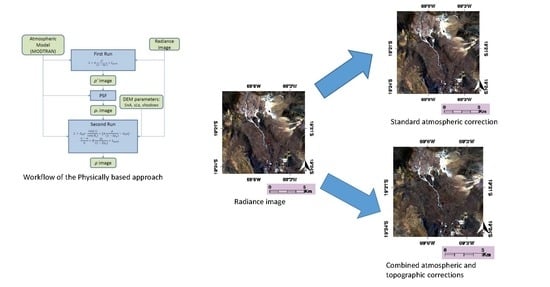
To properly estimate ρ, ρe should be estimated first. As a matter of fact, ρ is required to estimate ρe. For this reason, two correction steps are required. Thus, in the implemented schema, a first correction run is applied taking into consideration the model of Equation (1), which does not include the topographic correction. In this first run, the atmospheric column height is considered constant (DEM not included in the MODTRAN simulation). Applying the PSF, described in the previous chapter, to the reflectance obtained from this first run, ρe is obtained to be used in the second run. The second run applies to the model of Equation (11), which includes the elevation model and the adjacency effects, and gives ρ in the output. In Figure 2 a schematic representation of the algorithm flow is shown.
3. Data and Test Cases Description
The presented method was applied to several satellite and airborne images acquired under different acquisition and illumination geometry and showed high potentials in the topographic homogenization of sloping terrain, maintaining optimal levels of secondary effect corrections such as an adjacency effect. However, although topographic correction is always evident as a clear flattening of the image, it is not always easy to quantify its performance and impact on remotely sensing applications. The main difficulties are related to the poor knowledge of the soil covers and to the lack of wide homogenous areas over differently exposed slopes. Moreover, statistical methods applied over wide areas are affected by a physiological dependency of the classes on the slopes, especially in correspondence with the vegetation classes, due to the different exposition to the sun and the wind.
For this reasons, different methods and different test areas were used to highlight the improvement of data quality and the impact of the correction on remote sensing applications, basing on spectral comparisons and statistical considerations.
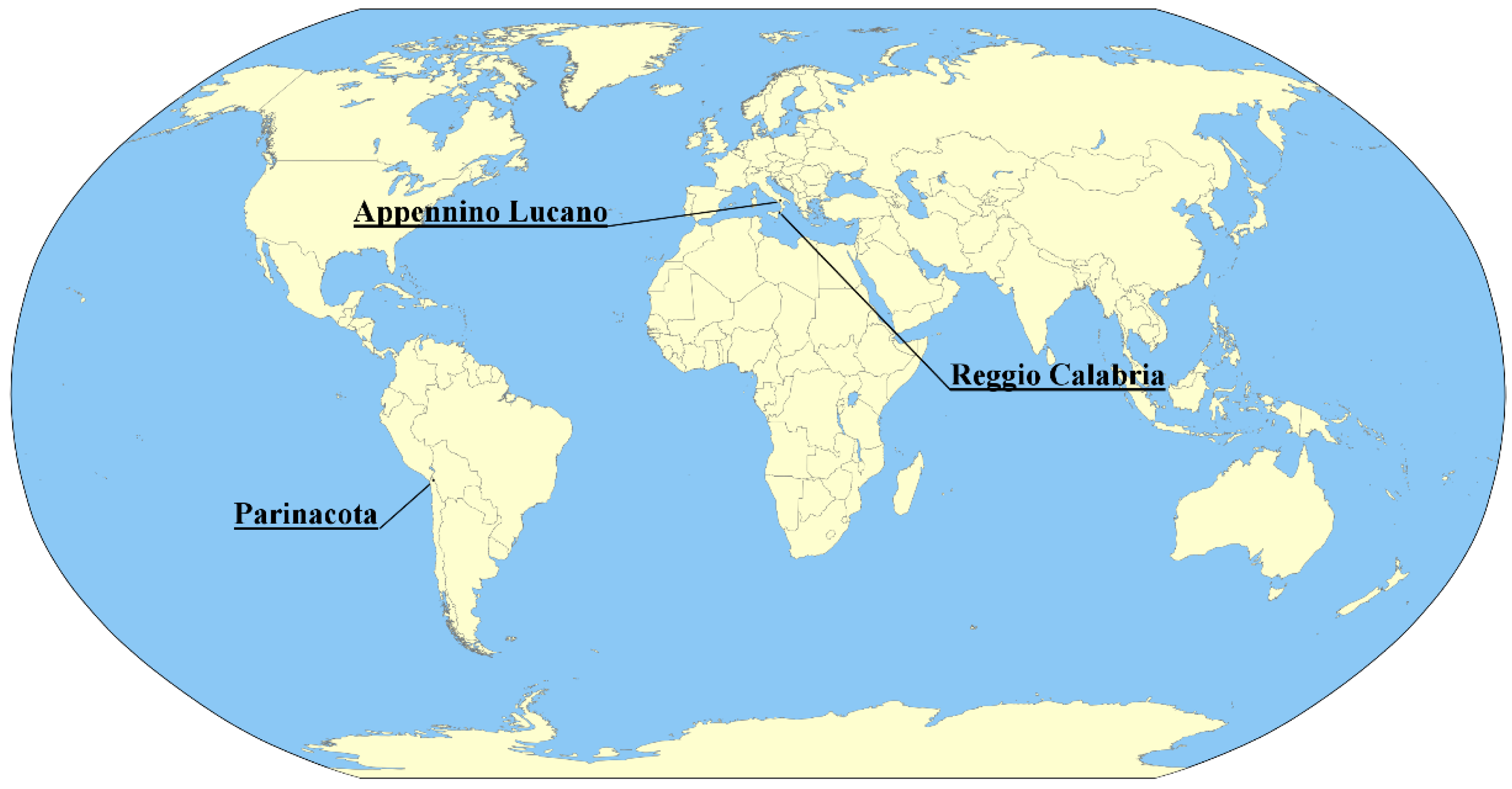
3.1. Appennino Lucano
The first test case was located within the “Appennino Lucano National Park”, a protected mountainous area of the Basilicata region, Italy (Figure 3), characterized by a considerable heterogeneity of soil covers. Thanks to this characteristic, the test case was exploited to evaluate the potential of the method in relation to remote sensing applications, using two cloudless subsets (centered at 40° 10’ 0″N, 16° 0′ 0″E and 40° 17′ 0″N, 15° 57′ 0″E) of a LANDASAT-8 image acquired on 2015/08/13 at 9:34 UTC available on the USGS (United States Geological Survey) Earthexplorer website, and a 5 m spatial resolution DEM issued by the cartographic institute of Basilicata.
Although, as will be shown in the next chapters, the correction procedure is clearly effective to the correction of both topographic and adjacency effects, due to the presence of vegetation covers, the impact of solar exposure makes the site not fully reliable for the generalization of the statistical analysis related to the standardization of terrain slopes. Thus, the second test case was placed in a very arid location in the Parinacota region of Chile, within the Andean mountains (Figure 3).
3.2. Andes, Parinacota
This test case was allowed to deepen the statistical analysis and quantify the impact of the topographic correction by calculating the increase of the similarity, after the correction, between two LANDSAT-8 subset images acquired in different seasons (different illumination geometries) on the same location (centered at 19° 20′ 0″S, 69° 6′ 0″W).
The images were acquired on 4/06/2016 (southern hemisphere winter) at 14:35 UTC and on 21/11/2016 (southern hemisphere summer) at 14:35 UTC, and were exploited using the 1 arc-second resolution global SRTM DEM. Both images and DEM were downloaded from Earthexplorer.
3.3. Reggio Calabria
Finally, the third test case was represented by a composite scenario, including a mountainous region (37° 57′ 41″N, 15° 40′ 45″E) and an industrial area (37° 56′ 57″N, 15° 42′ 3″E), in the province of Reggio Calabria (Calabria, Italy; Figure 3). The area was acquired on 2013 January the 8th at 8:30 UTC by a CASI sensor installed onboard an airborne platform at 1240 m above sea level, corresponding to a spatial resolution of 0.50 m at ground level. To make the most of the data, a DEM with a resolution of 1 m was used. Both CASI data and DEM were kindly granted by the Territorial Information Services (SIT) for the management of emergencies of the Calabria Region.
Given the very low sun illumination angle at the time of the CASI acquisition and the high spatial resolution of the data, this area allowed us to test the performance of the method in extreme conditions and its potential in the correction of shadows also in urban/industrial scenarios.
4. Results and Discussion
4.1. MODTRAN Test
Before applying the method to real test cases, it was tested on MODTRAN simulated data for self-consistency check. As MODTRAN simulations correspond to a homogeneous surface, the model, in this test, behaves like in its simplest formulation (Equation (1)).
A set of synthetic at sensor radiance images were created varying the albedo between 0.2 and 0.9 and the visibility between 1 km and 120 km and considering a sun-synchronous orbiting sensor with a spectral sampling of 10 nm and FWHM (Full Width at Half Maximum) of 20 nm. The atmosphere has been characterized by “rural aerosol” and “mid latitude winter” MODTRAN standard models, and the sun zenith angle was set to 40°.
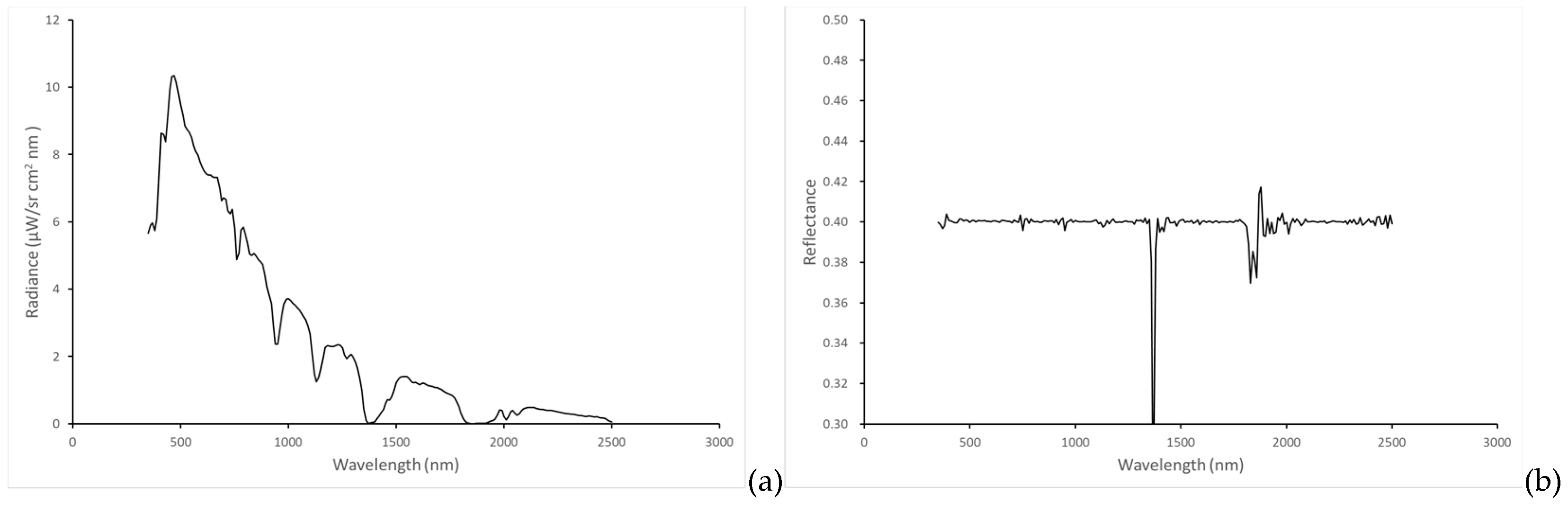
In Figure 4a, the simulated at sensor spectral radiance corresponding to the albedo 0.4 is shown, while Figure 4b depicts the reflectance spectrum obtained by applying the atmospheric correction to the synthetic data.
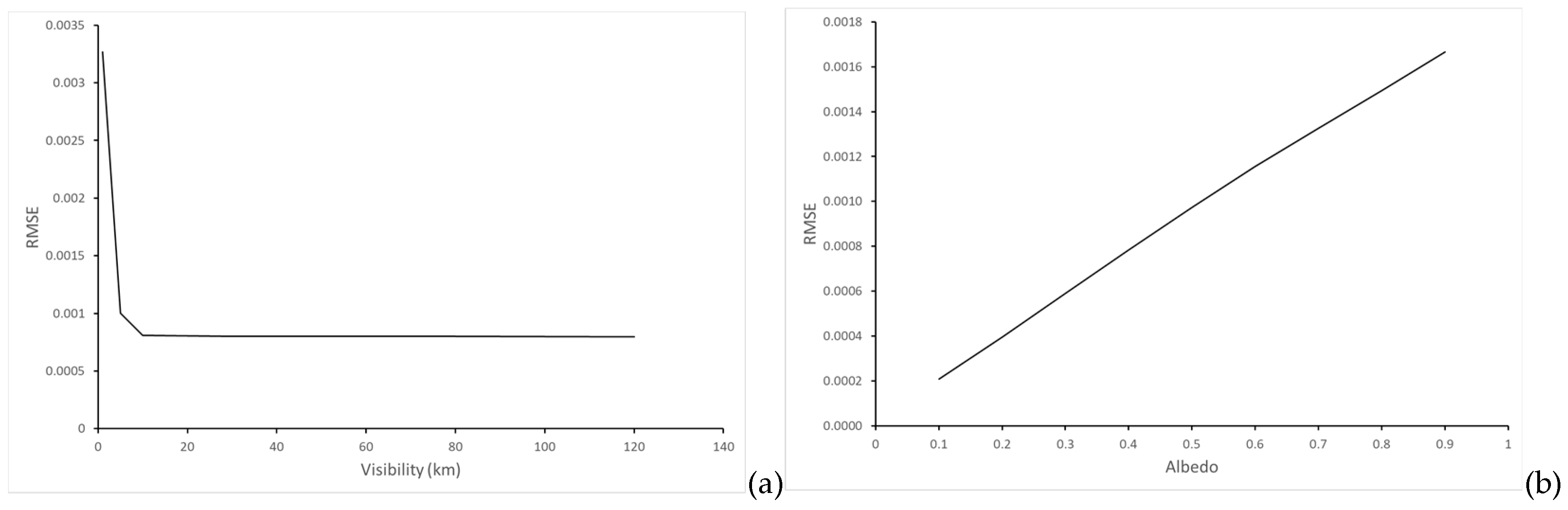
After having excluded the water absorption wavelengths, the RMSE (Root Mean Square Error) between the flat grey spectra corresponding to each albedo value and the related reflectance spectrum obtained by the application of the atmospheric correction was computed. Results show that the RMSE had a linear relation with the albedo and never exceeded the 2% of the albedo for visibility values above 10 km as seen from Figure 5 that shows the RMSE dependence on the visibility for an albedo of 0.4 (Figure 5a) and the RMSE dependence on the albedo for a visibility of 30 km (Figure 5b).
4.2. Appennino Lucano
As regards to the Appennino Lucano test case, Figure 6 shows two false color reflectance images obtained by the LANDSAT-8 radiance, excluding (Figure 6a) and including (Figure 6b) the topographic correction in the correction scheme. The angle between the incoming solar radiation and the normal to the surface derived from the DEM is shown on Figure 6c. Coherently with location and acquisition time, “rural aerosol” and “mid latitude summer” were selected in MODTRAN to model the aerosols. The visibility was selected on the bases of the nearest AERONET station located in Potenza, Basilicata. The figure clearly illustrates the flattening of the scene after the topographic correction and the loss of dependence from the slopes. This effect is particularly evident in the zoomed area (yellow square of Figure 6c).
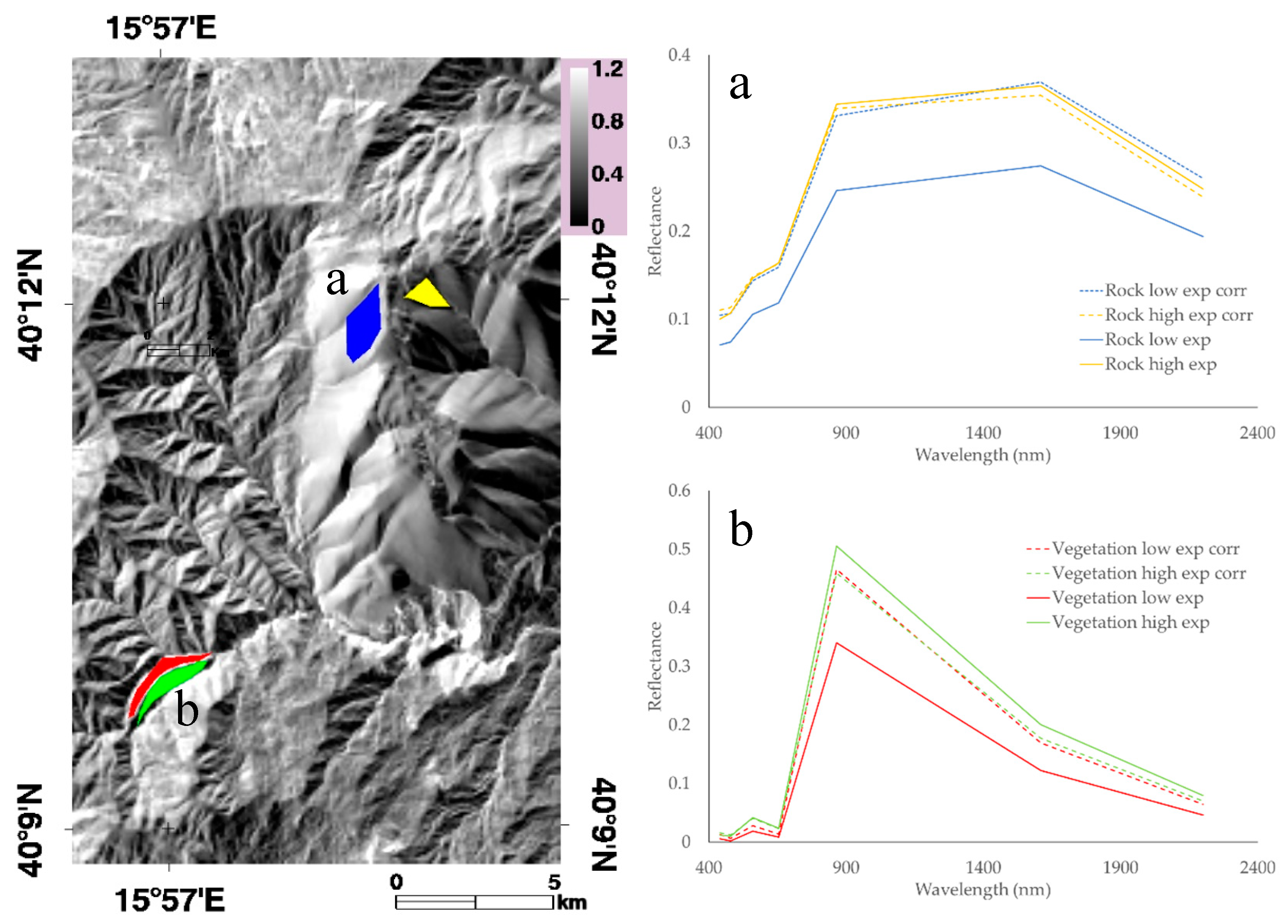
To quantify the impact of topographic correction, two homogeneous areas corresponding to rock and vegetation classes were identified. For each class, two ROIs (Region Of Interest) characterized by different sun expositions were outlined. Figure 7 shows, besides the location of the ROIs, the mean spectra of the ROIs organized into two graphs corresponding to the rock (Figure 7a) and vegetation (Figure 7b) classes. The solid line represents the spectrum before the topographic correction, the dashed line represents the same spectrum after the application of the topographic correction.
Analogously to what was found by Guanter et al. [32] and Richter and Schläpfer [34], the graphs clearly illustrate the high increase of the similarity between the spectra after topographic correction, being the dashed spectra nearly overlapping both for the rock and for the vegetation classes.
The increase of the spectral similarity between two spectra ( and ) was quantified by means of the normalized spectral distance (nsd), built on the bases of the RMS (root mean square):
A consistent improvement of the spectral similarity was observed after the topographic correction for both vegetation and rock classes. In fact, before the correction the nsd was 0.41 for the vegetation class and 0.30 for the rock class, while, after the correction, the values of the spectral distance lowered respectively to 0.04 and 0.05.
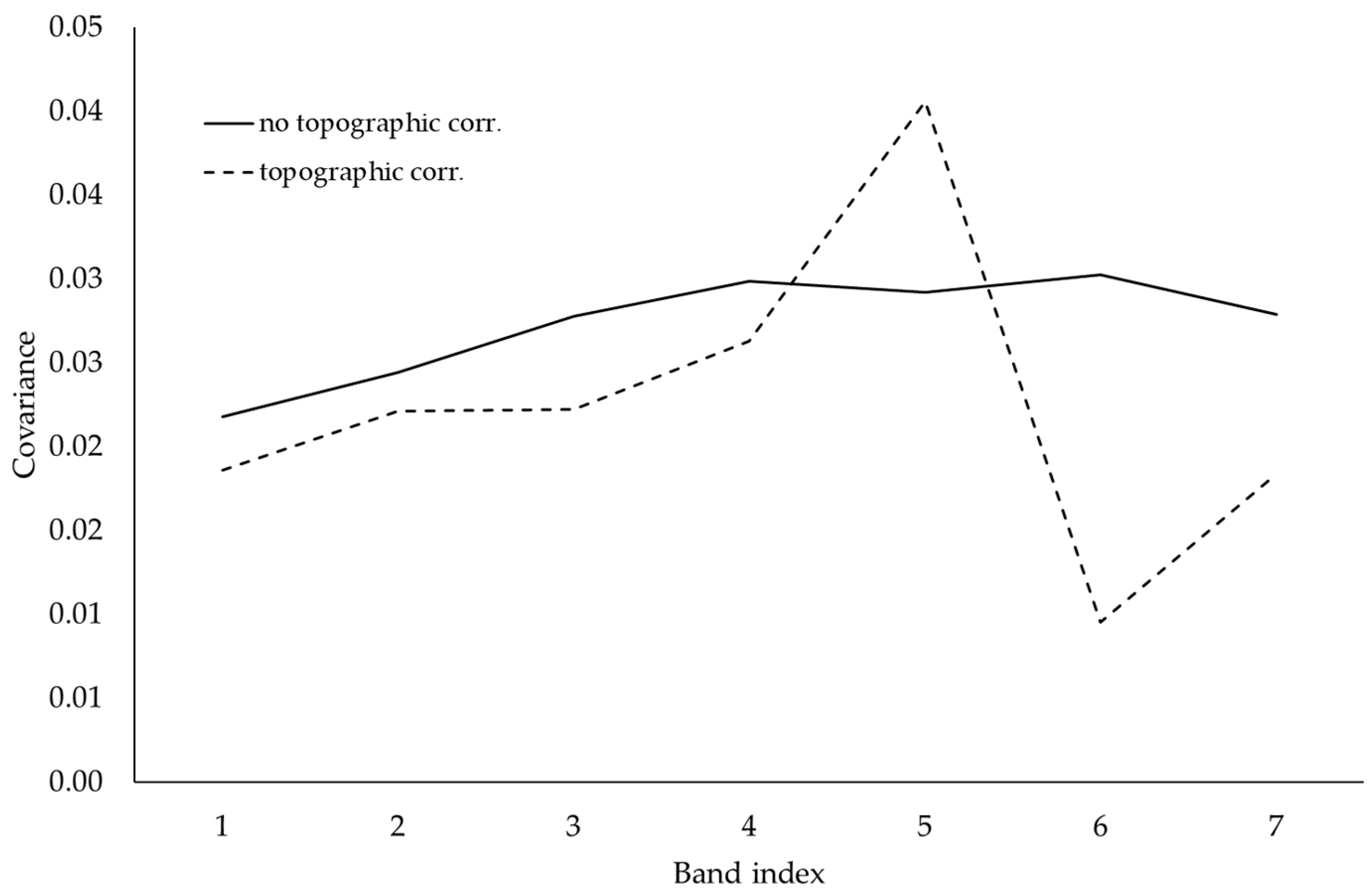
To estimate the whole improvement of the image, the correlation between the reflectance image and the sun exposition angle was computed before and after the inclusion of topographic correction [25]. Figure 8 shows the decrease of the correlation with the slopes after the topographic correction for all bands except for band 5, corresponding to the near infrared range (851–879 nm). This can be partially explained by the high sensitivity of the vegetation classes in this interval, which could be the expression of a physiological dependence of the vegetation classes on solar exposure.
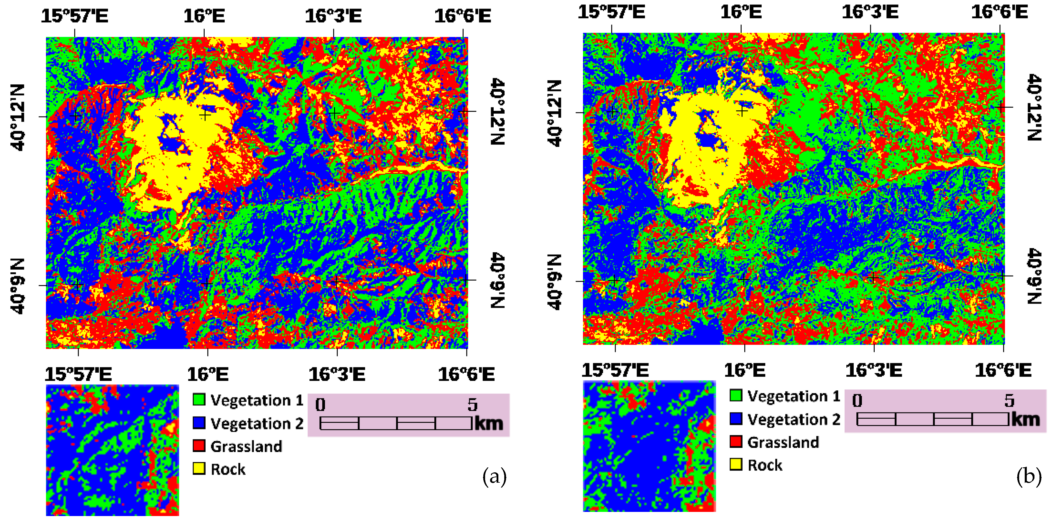
To assess the impact of such an improvement on remote sensing applications, an unsupervised k-means classification was applied, using four classes and a maximum of 100 iterations, before and after topographic correction. From a comparison with google images, the four classes can be easily interpreted as two vegetation classes, a rock class and a grassland class.
The results showed a general flattening of the classification image after slope correction with less visible mountain profiles and a general loss of the dependence on DEM features (Figure 9).
Further, with a few exceptions (bold values of Table 2), a general decrease of the image variance within each of the four classes after topographic correction was observed [22,25,44].
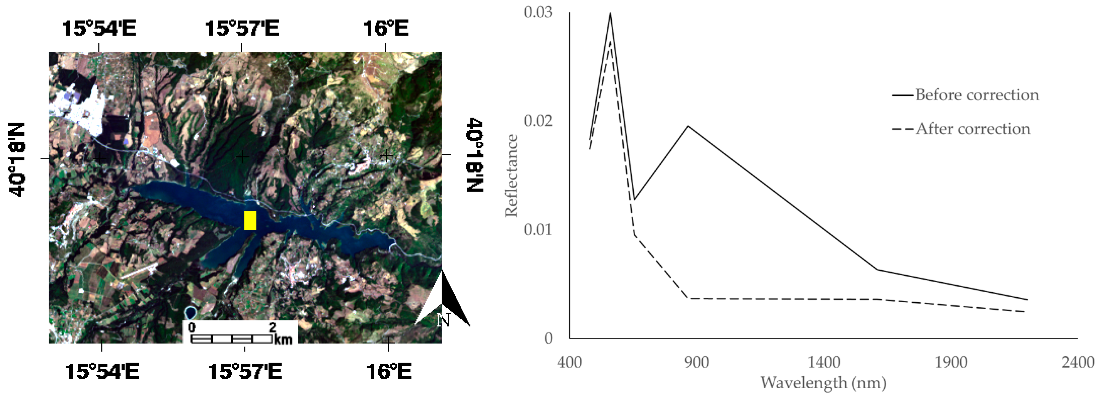
Before moving on the next test case, it is worth remarking the effectiveness of the method to the correction of environmental effects and the potential of processing data with a single and consistent model. On Figure 10, another subset of the same LANDSAT image depicts the Pertusillo Lake, a small inland water body that is surrounded by flourishing vegetation in the period in which the data were acquired. In the same figure, the graph shows the mean spectrum of a ROI (yellow rectangular) corresponding to deep water in the center of the lake before (solid line) adjacency and topographic corrections and after (dashed line) the comprehensive correction.
The graph clearly shows that the presence of vegetation causes a strong adjacency effect on the water body, especially on the band 5, corresponding to the near-infrared peak of vegetation and to a range in which the water should almost show no signal due to water column absorption [3]. After the comprehensive correction, the impact of adjacency effect of the surrounding vegetation is greatly reduced, and the spectrum returns to behave like a water spectrum in the infrared range.
4.3. Andes, Parinacota
The arid climate of the Andes region determines the almost total absence of vegetation classes and allowed us to suppose that no appreciable coverage changes had occurred between the winter and summer images. Therefore, if a good topographic correction is applied, the similarity between the two images is expected to increase after the correction due to the homogenization of the terrain illumination. The similarity was estimated by means of an nsd image obtained by applying pixel per pixel Equation (23) to the winter and summer images. The nsd image was calculated before and after topographic correction.
The atmospheric correction was carried out testing both rural and desertic aerosols and varying the horizontal visibility within 5 km and 120 km. Mid-latitude winter and mid-latitude summer aerosol models were used respectively for the winter and summer images. The results always show a marked improvement after topographic correction. The shown results concern the maximum similarity reached both before and after the topographic correction. In Figure 11, the nsd images obtained excluding (Figure 11a) and including (Figure 11b) the topographic corrections are shown besides the i angle derived from the DEM (Figure 11c). Also in this case, the flattening of the image and the loss of dependence on DEM parameters after the topographic correction is remarkable.
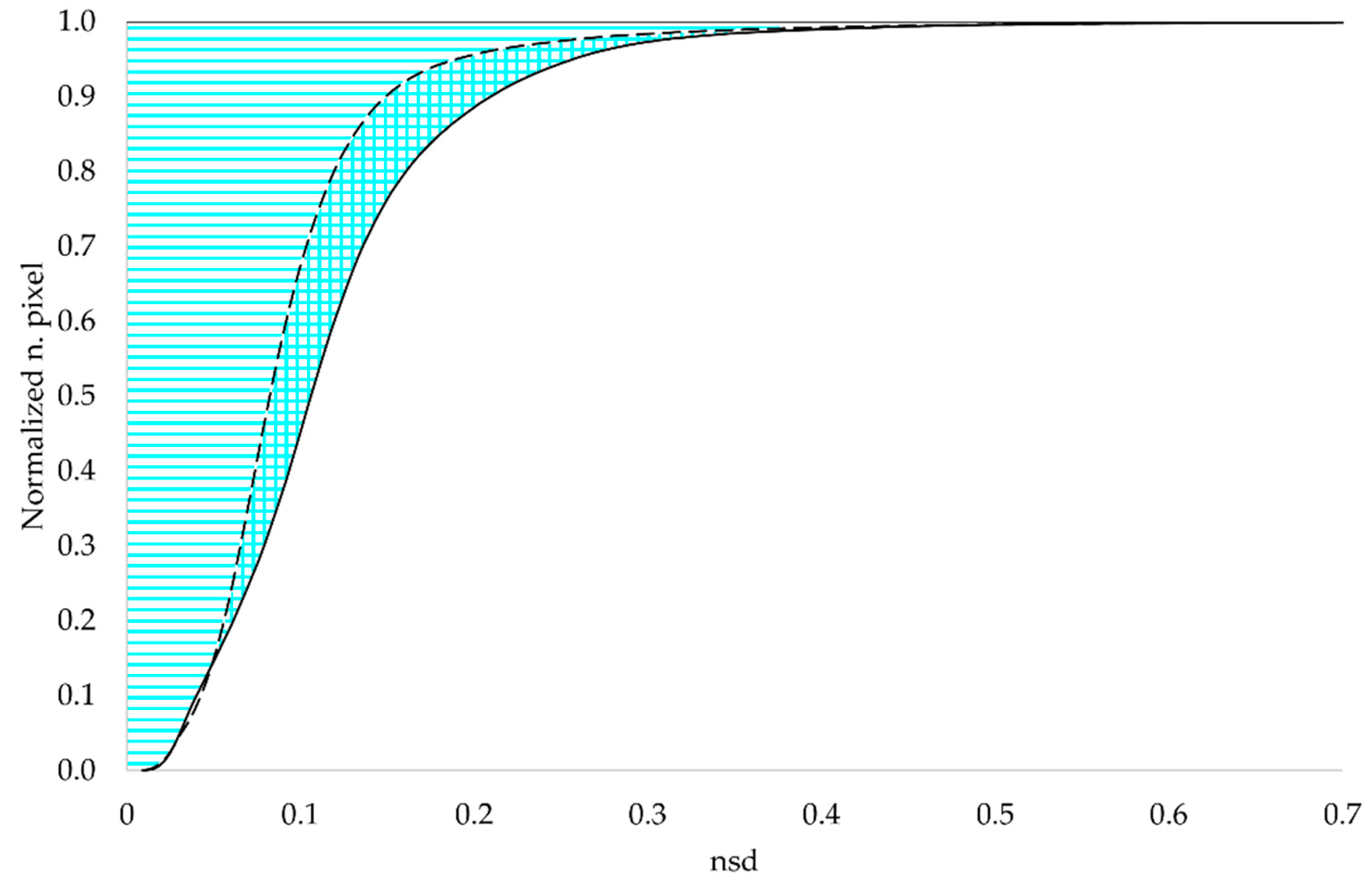
To quantify the increase in similarity, the cumulative function, which represents the fraction of pixels (ordinated in Figure 12) lower than a certain nsd value (abscissa in Figure 12), was computed both for the nsd image before topographic correction (solid line in Figure 12) and for the nsd image after topographic correction (dashed line in Figure 12). The graph depicted in Figure 12 shows the clear increment of the similarity between the winter and summer images after topographic correction, with over 85% of pixels within a distance of nsd = 0.15, compared to 75% when topographic corrections were not applied. A global measure of the improvement could be obtained by calculating the ratio between the area within the two curves (squared area in Figure 12) and the area above the blue curve (banded and squared areas in Figure 12), showing a reduction of over 15% of the difference between the winter and the summer image after topographic correction.
4.4. Reggio Calabria Test Case
The Reggio Calabria test case was useful to experiment with the method in an extreme condition. The very low sun zenith angle during acquisition time determined a high contrast and shadows. The correction was carried out considering high visibility, “rural aerosol” and “mid latitude winter” to implement the atmospheric model in MODTRAN. Results were remarkable, allowing the recovering, for most bands, of the signal even in the shade, both in industrial and mountain contexts.
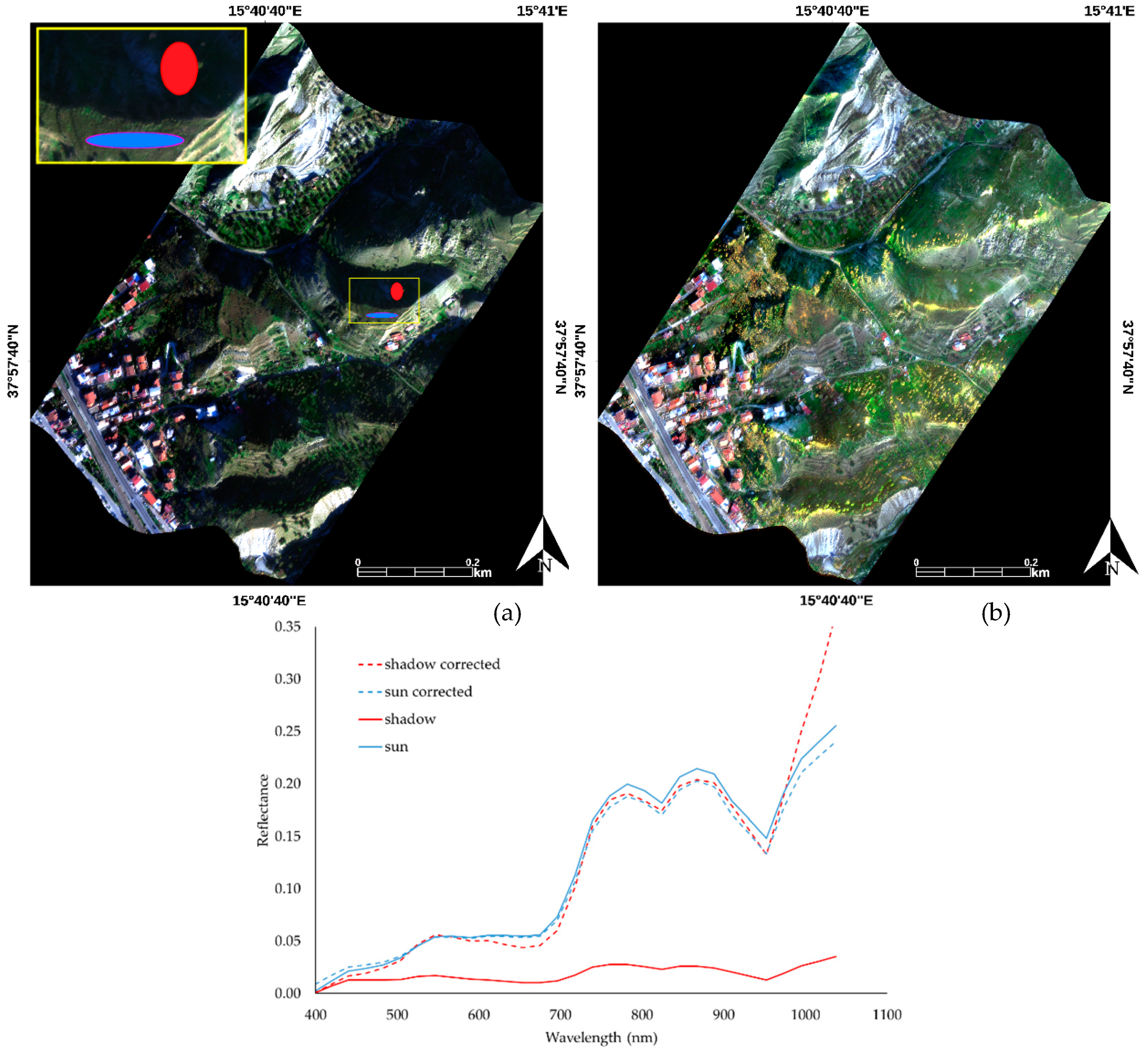
Analogously to what was done for the Appenino Lucano test case, the mean spectra of two ROIs, relating to shaded and exposed areas, were compared before and after the application of topographic corrections. For the industrial context the ROIs were located on a paved road partially shaded by a wall. For the mountain context, the ROIs were located on a shaded and an exposed slope. Figure 14a,b show respectively the RGB images before and after the topographic corrections for the industrial context, while Figure 15a,b show the RGB images before and after the topographic corrections for the mountain context. The graphs with the behavior of the mean spectra of the ROIs are shown on Figure 14c and Figure 15c respectively for the industrial and the mountain contexts.
For both subsets, a very low signal is observed for the shaded areas, which is largely recovered when the topographic correction is included in the correction procedure. For the industrial context, the shadow is very sharp and, due to the instrumental noise combined with the exponential decrease of the diffuse radiance, the signal is not recovered above 900 nm. The nsd, in the range 0–900 nm, passes from 1.42 before correction to 0.15 after correction. For the mountain context, the nsd (calculated over the whole range) goes from 1.53 before the correction to 0.19 after correction.
It must be said that these results are achievable only for airborne acquisitions. In the case of satellite observations, in fact, shadow corrections are much less efficient due to the absorption along the atmospheric column, which almost leads to a complete reset of the signal.
5. Conclusions
The paper shows an advanced and consistent physically based correction method that, under the assumption of Lambertian surface and isotropic sky irradiance, allows for atmospheric correction of remote sensing data, including second order corrections such as adjacency effects, and simultaneously compensating for illumination gradients due to mountain slopes. The method showed great potential in the improvement of remotely sensed products and was successfully used for shadow correction even in urban context when applied to airborne data. Further efforts are currently being made to personalize the model of the atmospheric column, to overcome the limitation of Lambertian surface, and to modify the sky factor in order to include the reflected light coming from the ground that replaces the irradiance coming from the portion of the sky dome that does not reach the sloped surface.
Author Contributions
Both authors have contributed to scientific investigation and to the conceptualisation of the paper, to data analysis and to the drafting of the document.
Funding
This research received no external funding
Acknowledgments
The authors would like to thank the SIT for providing CASI data and the associated DEM for the Reggio Calabria area, the USGS for providing Lansat images and the DEM of south America, and the cartographic institute of Basilicata for providing the DEM of the Basilicata region.
Conflicts of Interest
The authors declare no conflict of interest.
References
- Guanter, L.; Del Carmen, M.; Sanpedro, G.; Moreno, J. A method for the atmospheric correction of ENVISAT/MERIS data over land targets. Int. J. Remote Sens. 2007, 28, 709–728. [Google Scholar] [CrossRef]
- Acito, N.; Diani, M. Unsupervised atmospheric compensation of airborne hyperspectral images in the vnir spectral range. IEEE Trans. Geosci. Remote Sens. 2018, 56, 2083–2106. [Google Scholar] [CrossRef]
- Santini, F.; Alberotanza, L.; Cavalli, R.M.; Pignatti, S. A two-step optimization procedure for assessing water constituent concentrations by hyperspectral remote sensing techniques: An application to the highly turbid Venice lagoon waters. Remote Sens. Environ. 2010, 114, 887–898. [Google Scholar] [CrossRef]
- Amato, U.; Cavalli, R.M.; Palombo, A.; Pignatti, S.; Santini, F. Experimental approach to the selection of the components in the minimum noise fraction. IEEE Trans. Geosci. Remote Sens. 2009, 47, 153–160. [Google Scholar] [CrossRef]
- Hantson, S.; Chuvieco, E. Evaluation of different topographic correction methods for Landsat imagery. Int. J. Appl. Earth Obs. Geoinf. 2011, 13, 691–700. [Google Scholar] [CrossRef]
- Kawishwar, P. Atmospheric Correction Models for Retrievals of Calibrated Spectral Profiles from Hyperion EO-1 Data. Master’s Thesis, International Institute for Geo-Information Science and Earth Observation, Enschede, The Netherlands, 2007. [Google Scholar]
- Shepherd, J.D.; Dymond, J.R. Correcting satellite imagery for the variance of reflectance and illumination with topography. Int. J. Remote Sens. 2003, 24, 3503–3514. [Google Scholar] [CrossRef]
- Gao, Y.; Zhang, W. A simple empirical topographic correction method for ETM+ imagery. Int. J. Remote Sens. 2009, 30, 2259–2275. [Google Scholar] [CrossRef]
- Nichol, J.; Hang, L.K.; Sing, W.M. Empirical correction of low Sun angle images in steeply sloping terrain: A slope-matching technique. Int. J. Remote Sens. 2006, 27, 629–635. [Google Scholar] [CrossRef]
- Holben, B.N.; Justice, C.O. An examination of spectral band ratioing to reduce the topographic effect on remotely-sensed data. Int. J. Remote Sens. 1981, 2, 115–123. [Google Scholar] [CrossRef]
- Li, A.; Wang, Q.; Bian, J.; Lei, G. An Improved Physics-Based Model for Topographic Correction of Landsat TM Images. Remote Sens. 2015, 7, 6296–6319. [Google Scholar] [CrossRef] [Green Version]
- Conese, C.; Maracci, G.; Maselli, F. Improvement in maximum likelihood classification performance on highly rugged terrain using principal component analysis. Int. J. Remote Sens. 1993, 14, 1371–1382. [Google Scholar] [CrossRef]
- Pouch, G.W.; Campagna, D.J. Hyperspherical direction cosine transformation for separation of spectral and illumination information in digital scanner data. Photogramm. Eng. Remote Sens. 1990, 56, 475–479. [Google Scholar]
- Füreder, P. Topographic correction of satellite images for improved LULC classification in alpine areas. In Proceedings of the 10th International Symposium on High Mountain Remote Sensing Cartography, International Centre for Integrated Mountain Development (ICIMOD), Kathmandu, Nepal, 8–11 September 2008; Kaufmann, V., Sulzer, W., Eds.; Institute of Geography and Regional Science, University of Graz: Graz, Austria, 2010; pp. 187–194. [Google Scholar]
- Law, K.H.; Nichol, J.E. Topographic correction for differential illumination effects on IKONOS satellite imagery. Int. Arch. Photogramm. Remote Sens. Spat. Inform. Sci. 2004, 35, 641–646. [Google Scholar]
- Feng, J.; Rivard, B.; Sánchez-Azofeifa, A. The topographic normalization of hyperspectral data: Implications for the selection of spectral end members and lithologic mapping. Remote Sens. Environ. 2003, 85, 221–231. [Google Scholar] [CrossRef]
- Hale, S.R.; Rock, B.N. Impact of topographic normalization on land-cover classification accuracy. Photogramm. Eng. Remote Sens. 2003, 69, 785–791. [Google Scholar] [CrossRef]
- Tokola, T.; Sarkeala, J.; Van der Linden, M. Use of topographic correction in Landsat TM-based forest interpretation in Nepal. Int. J. Remote Sens. 2001, 22, 551–563. [Google Scholar] [CrossRef]
- Vincini, M.; Frazzi, E. Multitemporal evaluation of topographic normalization methods on deciduous forest TM data. IEEE Trans. Geosci. Remote Sens. 2003, 41, 2586–2590. [Google Scholar] [CrossRef]
- Gu, D.; Gillespie, A. Topographic normalization of Landsat TM images of forest based on subpixel sun–canopy–sensor geometry. Remote Sens. Environ. 1998, 64, 166–175. [Google Scholar] [CrossRef]
- Colby, J.D. Topographic normalization in rugged terrain. Photogramm. Eng. Remote Sens. 1991, 57, 531–537. [Google Scholar]
- Richter, R.; Kellenberger, T.; Kaufmann, H. Comparison of topographic correction methods. Remote Sens. 2009, 1, 184–196. [Google Scholar] [CrossRef]
- McDonald, E.R.; Wu, X.; Caccetta, P.; Campbell, N. Illumination correction of Landsat TM data in south east NSW. Environ. Aust. 2002, 22, 19–23. [Google Scholar]
- Meyer, P.; Itten, K.I.; Kellenberger, T.; Sandmeier, S.; Sandmeier, R. Radiometric corrections of topographically induced effects on Landsat TM data in an alpine environment. ISPRS J. Photogramm. Remote Sens. 1993, 48, 17–28. [Google Scholar] [CrossRef]
- Wu, Q.; Jin, Y.; Fan, H. Evaluating and comparing performances of topographic correction methods based on multi-source DEMs and Landsat-8 OLI data. Int. J. Remote Sens. 2016, 37, 4712–4730. [Google Scholar] [CrossRef]
- Richter, R. Correction of atmospheric and topographic effects for high spatial resolution satellite imagery. Int. J. Remote Sens. 1997, 18, 1099–1111. [Google Scholar] [CrossRef]
- Sandmeier, S.; Itten, K.I. A physically-based model to correct atmospheric and illumination effects in optical satellite data of rugged terrain. IEEE Trans. Geosci. Remote Sens. 1997, 35, 708–717. [Google Scholar] [CrossRef] [Green Version]
- Sirguey, P. Simple correction of multiple reflection effects in rugged terrain. Int. J. Remote Sens. 2009, 30, 1075–1081. [Google Scholar] [CrossRef]
- Sirguey, P.; Mathieu, R.; Arnaud, Y. Subpixel monitoring of the seasonal snow cover with MODIS at 250 m spatial resolution in the Southern Alps of New Zealand, Methodology and accuracy assessment. Remote Sens. Environ. 2009, 113, 160–181. [Google Scholar] [CrossRef]
- Yin, G.; Li, A.; Zhao, W.; Jin, H.; Bian, J.; Wu, S. Modeling Canopy Reflectance Over Sloping Terrain Based on Path Length Correction. IEEE Trans. Geosci. Remote Sens. 2017, 55, 4597–4690. [Google Scholar] [CrossRef]
- Guanter, L.; Kaufmann, H.; Segl, K.; Foerster, S.; Rogass, C.; Chabrillat, S.; Kuester, T.; Hollstein, A.; Rossner, G.; Chlebek, C.; et al. The EnMAP spaceborne imaging spectroscopy mission for Earth observation. Remote Sens. Environ. 2015, 7, 8830–8857. [Google Scholar] [CrossRef]
- Guanter, L.; Richter, R.; Kaufmann, H. On the application of the MODTRAN4 atmospheric radiative transfer code to optical remote sensing. Int. J. Remote Sens. 2009, 30, 1407–1424. [Google Scholar] [CrossRef]
- Kobayashi, S.; Sanga-Ngoie, K. The integrated radiometric correction of optical remote sensing imageries. Int. J. Remote Sens. 2008, 29, 5957–5985. [Google Scholar] [CrossRef]
- Richter, R.; Schläpfer, D. Geo-atmospheric processing of airborne imaging spectrometry data. Part 2: Atmospheric/topographic correction. Int. J. Remote Sens. 2002, 23, 2631–2649. [Google Scholar] [CrossRef]
- Richter, R. Correction of satellite imagery over mountainous terrain. Appl. Opt. 1998, 37, 4004–4015. [Google Scholar] [CrossRef]
- Vermote, E.F.; Tanré, D.; Deuze, J.L.; Herman, M.; Morcette, J.J. Second simulation of the satellite signal in the solar spectrum, 6S: An. overview. IEEE Trans. Geosci. Remote Sens. 1997, 35, 675–686. [Google Scholar] [CrossRef]
- Adler-Golden, S.M.; Matthew, M.W.; Bernstein, L.S.; Levine, R.Y.; Berk, A.; Richtsmeier, S.C.; Acharya, P.K.; Anderson, G.P.; Felde, G.; Gardner, J.; et al. Atmospheric correction for short-wave spectral imagery based on MODTRAN4. SPIE Proc. Imaging Spectrom. 1999, 3753, 61–69. [Google Scholar]
- Vermote, E.; Tanré, D.; Deuzé, J.L.; Herman, M.; Morcrette, J.J.; Kotchenova, S.Y. Second simulation of a satellite signal in the solar spectrum-vector (6SV). 6S User Guide Version 2006, 3, 1–55. [Google Scholar]
- Jensen, J.R. Introduction Digital Image Processing: A Remote Sensing Perspective, 2nd ed.; Prentice-Hall: Englewood Cliffs, NJ, USA, 1996. [Google Scholar]
- Berk, A.; Anderson, G.P.; Acharya, P.K.; Chetwynd, J.H.; Bernstein, L.S.; Shettle, E.P.; Matthew, M.W.; Adler-Golden, S.M. Modtran4 User’s Manual; Air Force Research Laboratory: Hanscom AFB, MA, USA, 2000. [Google Scholar]
- 6SV Second Simulation of a Satellite Signal in the Solar Spectrum Vector Code. Available online: http://6s.ltdri.org/pages/downloads.html (accessed on 1 October 2016).
- Vermote, E.F.; Vermeulen, A. Atmospheric correction algorithm: Spectral reflectances (MOD09). ATBD Version 1999, 4, 1–107. [Google Scholar]
- Sanders, L.C.; Schott, J.R.; Raqueno, R. A VNIR/SWIR atmospheric correction algorithm for hyperspectral imagery with adjacency effect. Remote Sens. Environ. 2001, 78, 252–263. [Google Scholar] [CrossRef]
- Svoray, T.; Carmel, Y. Empirical method for topographic correction in aerial photographs. IEEE Geosci. Remote Sens. Lett. 2005, 2, 211–214. [Google Scholar] [CrossRef]
Figure 1.
Radiative transfer in the atmosphere/soil system.
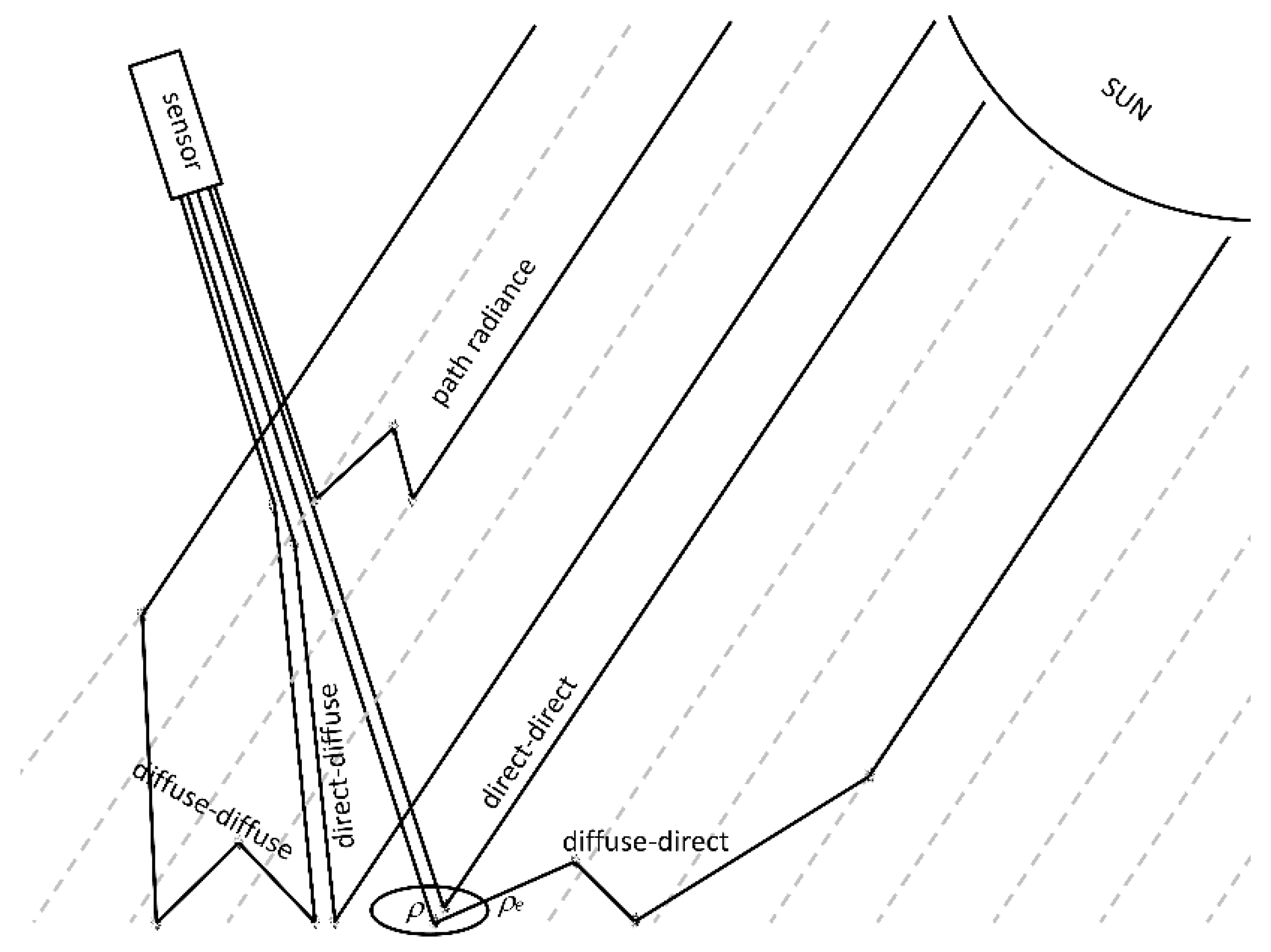
Figure 2.
Algorithm flow.
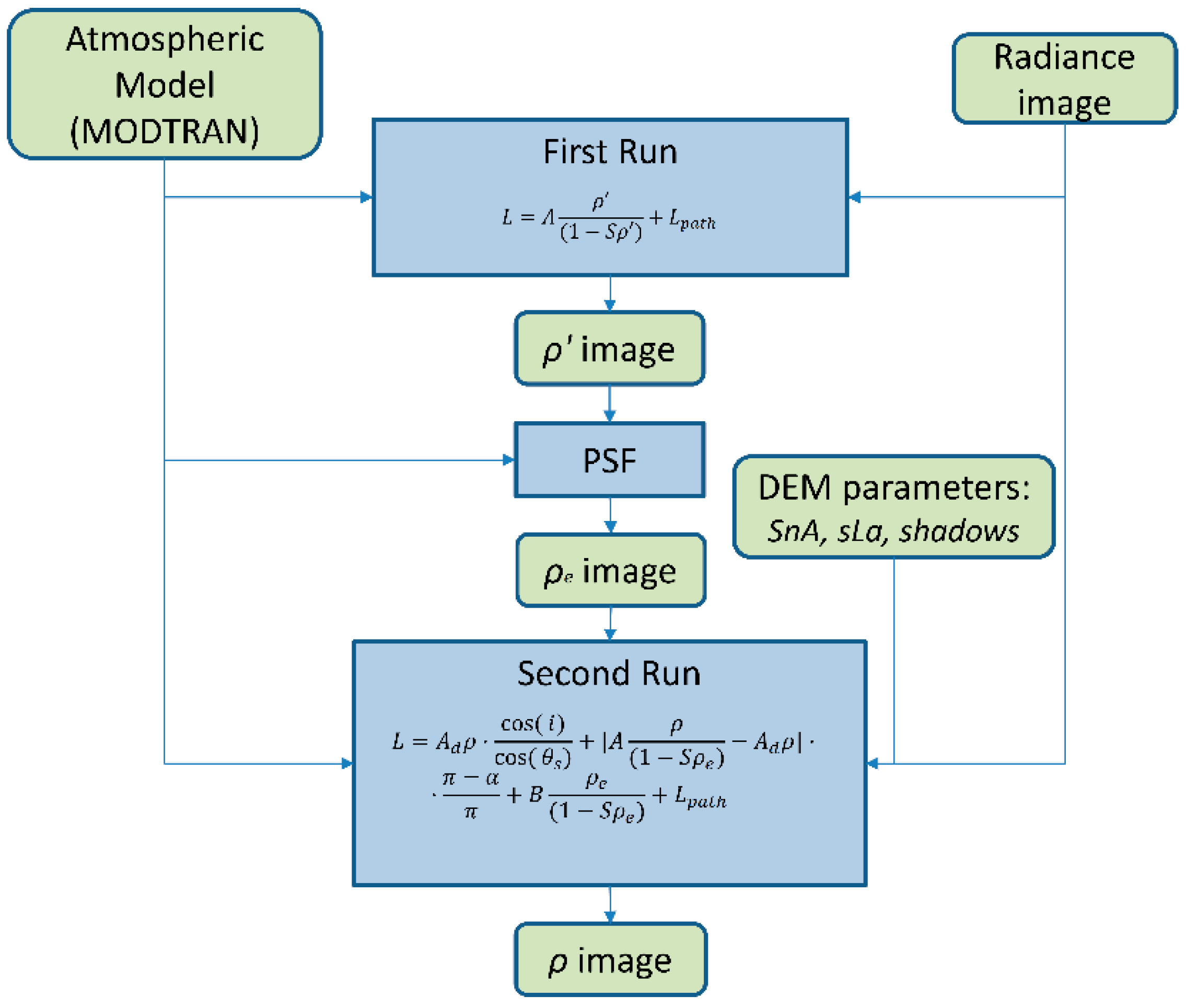
Figure 3.
Test cases locations.

Figure 4.
At sensor radiance simulated by MODTRAN corresponding to an albedo of 0.4 (a) and related atmospherically corrected spectrum (b).
Figure 4.
At sensor radiance simulated by MODTRAN corresponding to an albedo of 0.4 (a) and related atmospherically corrected spectrum (b).

Figure 5.
RMSE dependence on the visibility for an albedo of 0.4 (a), and on the albedo for a visibility of 30 km (b).
Figure 5.
RMSE dependence on the visibility for an albedo of 0.4 (a), and on the albedo for a visibility of 30 km (b).

Figure 6.
False color LANDSAT-8 images (R: 865 nm, G: 563 nm, B: 483 nm) before (a) and after (b) topographic correction; angle between the incoming solar radiation and the normal to the surface derived from the digital elevation model (DEM; c).
Figure 6.
False color LANDSAT-8 images (R: 865 nm, G: 563 nm, B: 483 nm) before (a) and after (b) topographic correction; angle between the incoming solar radiation and the normal to the surface derived from the digital elevation model (DEM; c).

Figure 7.
Location and mean spectra of the ROIs related to the rock (a) and vegetation (b) classes. The graphs show the mean spectra of the ROIs before (solid lines) and after (dashed lines) the inclusion of topographic corrections.
Figure 7.
Location and mean spectra of the ROIs related to the rock (a) and vegetation (b) classes. The graphs show the mean spectra of the ROIs before (solid lines) and after (dashed lines) the inclusion of topographic corrections.

Figure 8.
Correlation index between the reflectance image and the sun exposition before (blue line) and after (orange line) the topographic correction.
Figure 8.
Correlation index between the reflectance image and the sun exposition before (blue line) and after (orange line) the topographic correction.

Figure 9.
K-means maps obtained by setting four classes and a maximum of 100 iterations before (a) and after (b) topographic corrections.
Figure 9.
K-means maps obtained by setting four classes and a maximum of 100 iterations before (a) and after (b) topographic corrections.

Figure 10.
Landsat-8 image of Pertusillo Lake; in the graph, mean spectra of center lake deep water before (solid line) and after (dashed line) the application of the comprehensive correction procedure are shown.
Figure 10.
Landsat-8 image of Pertusillo Lake; in the graph, mean spectra of center lake deep water before (solid line) and after (dashed line) the application of the comprehensive correction procedure are shown.

Figure 11.
Normalized spectral distance (nsd) images before (a) and after (b) topographic correction; DEM derived angle between the incoming solar radiation and the normal to the surface related to the winter image (c).
Figure 11.
Normalized spectral distance (nsd) images before (a) and after (b) topographic correction; DEM derived angle between the incoming solar radiation and the normal to the surface related to the winter image (c).

Figure 12.
Nsd cumulative distribution before (solid line) and after (dashed line) the inclusion of topographic correction.
Figure 12.
Nsd cumulative distribution before (solid line) and after (dashed line) the inclusion of topographic correction.

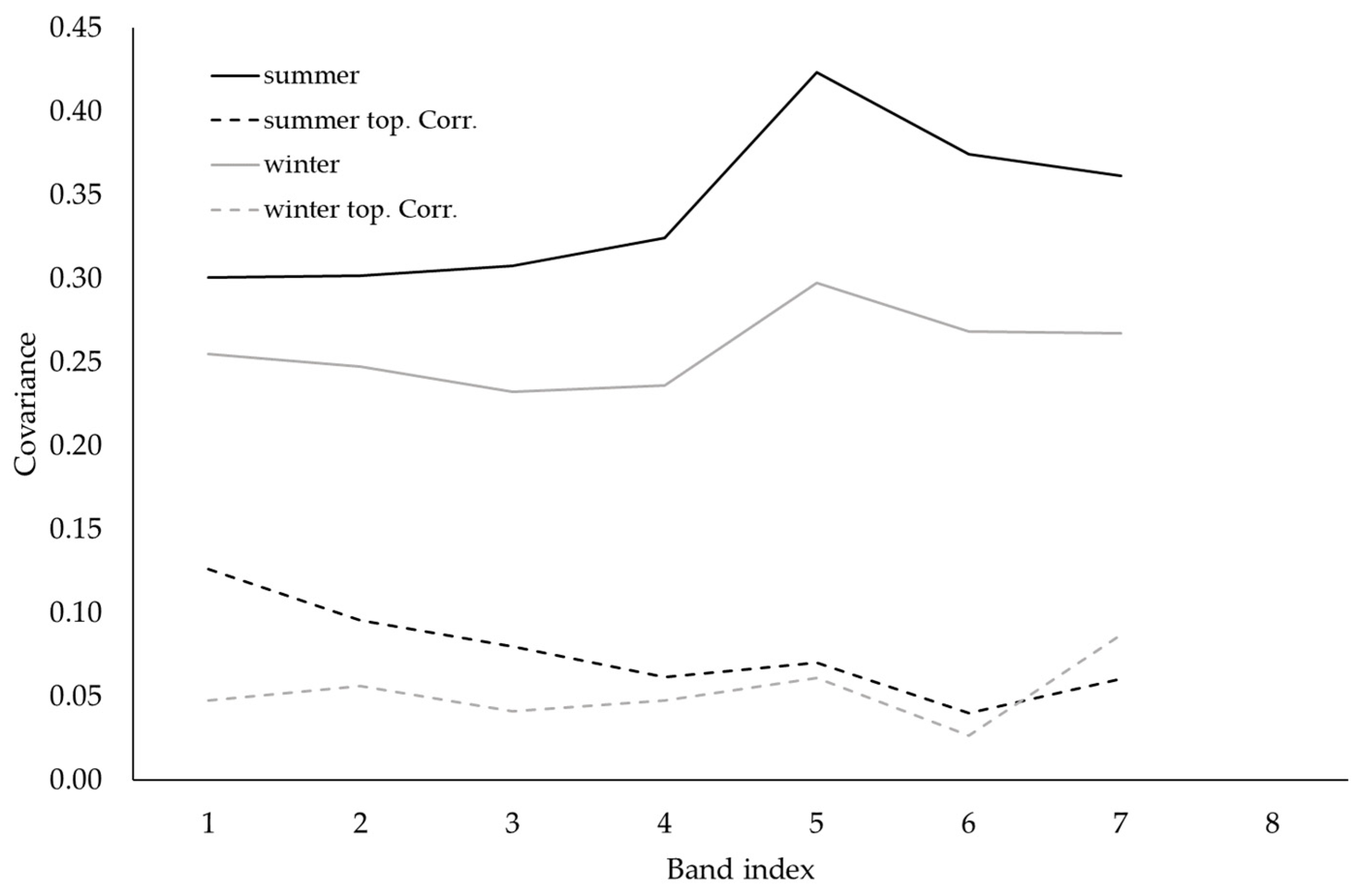
Figure 13.
Correlation index between the reflectance images and the sun exposition before (solid lines) and after (dashed lines) topographic correction.
Figure 13.
Correlation index between the reflectance images and the sun exposition before (solid lines) and after (dashed lines) topographic correction.

Figure 14.
RGB (R: 653 nm, G: 546 nm, B: 439 nm) images before (a) and after (b) the application of topographic correction related to a subsets of the Reggio Calabria CASI image, corresponding to an industrial context. The zoomed area in (a) highlights the ROIs relates to shadow (red) and exposed (blue) areas. On the graph the mean spectra of the two ROIs, before (solid lines) and after (dashed lines) the application of topographic corrections are shown.

Figure 15.
RGB (R: 653 nm, G: 546 nm, B: 439 nm) images before (a) and after (b) the application of topographic correction related to a subsets of the Reggio Calabria CASI image, corresponding to a mountain context. The zoomed area in (a) highlights the ROIs relates to shadow (red) and exposed (blue) areas. On the graph the mean spectra of the two ROIs, before (solid lines) and after (dashed lines) the application of topographic corrections are shown.

Table 1.
MODTRAN outputs used in the paper.
| MODTRAN Output Column (Output File Rootname.7sc) | MODTRAN Input Parameters (Input File Rootname.5tp) | Simulated Physical Quantity |
|---|---|---|
| GRND RFLT | SURREF≠0 in CARD 1 | Direct–direct + diffuse–direct contributions |
| DRCT RFLT | SURREF≠0 in CARD 1 | Direct–direct contribution |
| SOL SCAT | SURREF≠0 in CARD 1 | Direct–diffuse + diffuse–diffuse contributions + path radiance |
| SOL SCAT | SURREF=0 in CARD 1 | Path radiance (Lpath) |
Table 2.
Reflectance variance computed within the four cover classes excluding and including the topographic corrections. Bold values highlight the few values for wich an increase was observed after the inclusion of topographic corrections.
Table 2.
Reflectance variance computed within the four cover classes excluding and including the topographic corrections. Bold values highlight the few values for wich an increase was observed after the inclusion of topographic corrections.
| Veg. 1 | Veg. 2 | Grassland | Rock | Veg.1 | Veg.2 | Grassland | Rock | |
|---|---|---|---|---|---|---|---|---|
| Bands | no Topographic Correction | Topographic Correction | ||||||
| 1 (440 nm) | 0.006 | 0.006 | 0.010 | 0.021 | 0.005 | 0.005 | 0.009 | 0.020 |
| 2 (480 nm) | 0.007 | 0.006 | 0.010 | 0.021 | 0.006 | 0.005 | 0.010 | 0.020 |
| 3 (560 nm) | 0.009 | 0.010 | 0.011 | 0.024 | 0.009 | 0.009 | 0.012 | 0.021 |
| 4 (655 nm) | 0.011 | 0.009 | 0.017 | 0.026 | 0.010 | 0.008 | 0.017 | 0.023 |
| 5 (865 nm) | 0.033 | 0.039 | 0.039 | 0.043 | 0.031 | 0.042 | 0.033 | 0.045 |
| 6 (1610 nm) | 0.024 | 0.023 | 0.026 | 0.041 | 0.023 | 0.026 | 0.026 | 0.035 |
| 7 (2200 nm) | 0.015 | 0.014 | 0.021 | 0.034 | 0.015 | 0.015 | 0.021 | 0.030 |
© 2019 by the authors. Licensee MDPI, Basel, Switzerland. This article is an open access article distributed under the terms and conditions of the Creative Commons Attribution (CC BY) license (http://creativecommons.org/licenses/by/4.0/).
Share and Cite
MDPI and ACS Style
Santini, F.; Palombo, A. Physically Based Approach for Combined Atmospheric and Topographic Corrections. Remote Sens. 2019, 11, 1218. https://0-doi-org.brum.beds.ac.uk/10.3390/rs11101218
AMA Style
Santini F, Palombo A. Physically Based Approach for Combined Atmospheric and Topographic Corrections. Remote Sensing. 2019; 11(10):1218. https://0-doi-org.brum.beds.ac.uk/10.3390/rs11101218
Chicago/Turabian StyleSantini, Federico, and Angelo Palombo. 2019. "Physically Based Approach for Combined Atmospheric and Topographic Corrections" Remote Sensing 11, no. 10: 1218. https://0-doi-org.brum.beds.ac.uk/10.3390/rs11101218
Note that from the first issue of 2016, this journal uses article numbers instead of page numbers. See further details here.