Winter Wheat Canopy Height Extraction from UAV-Based Point Cloud Data with a Moving Cuboid Filter


Department of Geography, the University of Western Ontario, London, ON N6A 5C2, Canada
*
Author to whom correspondence should be addressed.
Remote Sens. 2019, 11(10), 1239; https://0-doi-org.brum.beds.ac.uk/10.3390/rs11101239
Submission received: 25 April 2019
/
Revised: 14 May 2019
/
Accepted: 22 May 2019
/
Published: 24 May 2019
(This article belongs to the Special Issue Advances of Multi-Temporal Remote Sensing in Vegetation and Agriculture Research)
Abstract
:Plant height can be used as an indicator to estimate crop phenology and biomass. The Unmanned Aerial Vehicle (UAV)-based point cloud data derived from photogrammetry methods contains the structural information of crops which could be used to retrieve crop height. However, removing noise and outliers from the UAV-based crop point cloud data for height extraction is challenging. The objective of this paper is to develop an alternative method for canopy height determination from UAV-based 3D point cloud datasets using a statistical analysis method and a moving cuboid filter to remove outliers. In this method, first, the point cloud data is divided into many 3D columns. Secondly, a moving cuboid filter is applied in each column and moved downward to eliminate noise points. The threshold of point numbers in the filter is calculated based on the distribution of points in the column. After applying the moving cuboid filter, the crop height is calculated from the highest and lowest points in each 3D column. The proposed method achieved high accuracy for height extraction with low Root Mean Square Error (RMSE) of 6.37 cm and Mean Absolute Error (MAE) of 5.07 cm. The canopy height monitoring window for winter wheat using this method starts from the beginning of the stem extension stage to the end of the heading stage (BBCH 31 to 65). Since the height of wheat has limited change after the heading stage, this method could be used to retrieve the crop height of winter wheat. In addition, this method only requires one operation of UAV in the field. It could be an effective method that can be widely used to help end-user to monitor their crops and support real-time decision making for farm management.

1. Introduction
The commercial applications of Unmanned Aerial Vehicle (UAV) systems in agriculture are emerging as a lucrative sector in the crop forecasting [1]. Many UAV-based applications help farmers by taking aerial images over an entire crop field, providing crucial data on crops and soil; these data assist farmers in crop management [2,3,4]. One of the most essential advantages of UAV applications in agriculture is that the intra-field variabilities of the development and health status in the crop can be monitored throughout the growing season with high spatial resolution images [5,6,7]. Also, UAV-based high temporal resolution images can provide real-time data, which offers farmers the opportunity to make well-informed decisions on farming activities [8]. Currently, several services can be available throughout the crop growing cycles using UAV-based remote sensing techniques, including two main categories: soil and field analysis and crop parameter monitoring. The applications of UAVs in soil and field analysis focus on field 3D mapping and assessment at the start of the crop season [9]. Real-time UAV data collection provides a better solution for precise crop monitoring, including the crop canopy leaf area index (LAI), nitrogen status, water stress, and biomass [3,10,11,12,13,14]. The UAV-based data fill the gap in remotely sensed data between ground-based measurements and conventional airborne and satellite data collection [15].
Crop height is an indicator of crop phenology, which can be used to predict crop biomass and final yield potential [16]. Accurate estimation of intra-field biomass variability requires subfield-scale plant height estimation. Hence, accurate plant height estimation at the subfield scale is desirable. One traditional approach to determine the height of an object via remote sensing is the photogrammetric method using a pair of stereo satellite images [17,18]. However, the spatial and temporal resolution of satellite images restricts the application of this method in frequent crop height determination [19]. Another approach is to estimate crop height using an airborne or ground-based LiDAR sensor [20,21]. LiDAR has the advantage of high accuracy; however, the costs are prohibitively high, making it difficult in practice. The third approach is to use a depth camera such as the Microsoft Kinect to estimate crop height from a derived crop surface model [22], but the range limit of measurement restricts the mapping of the entire field [23]. The fourth approach is manual measurement in the field, which requires a heavy workload and time consumption.
The recent development in UAV systems and computer vision has enabled the UAV-based remote sensing generation of dense 3D reconstructions to produce orthomosaics, digital surface model (DSM), and 3D point clouds using the Structure from Motion (SfM) approach [24,25,26,27]. SfM is a computer vision technique that incorporates multi-view stereo images to match features, derive 3D structure, and estimate camera position and orientation [28]. The 3D point clouds derived from UAV-based images are a set of 3D data points that contains the spatial information of features and have a similar format to LiDAR data [25,27]. Many studies have estimated crop canopy height and biomass from UAV-based images using the SfM approach [29,30,31,32,33,34,35,36].
Bendig et al. [33] presented a method that used multiple crop surface models (CSMs) derived from UAV-based imagery and the SfM technique to estimate crop canopy height throughout the crop growing season. The canopy height was determined by measuring the difference between the CSMs and the digital terrain model (DTM). By using this CSMs method, many studies estimated crop height from UAV digital images [37,38,39]. The advantages of this method are its accuracy and reliability for the entire crop growing season. However, the accuracy of the crop surface models and ground surface model are strongly related to the absolute accuracy of the 3D point cloud data, which is dependent on the number of images, the accuracy of the camera exterior and interior orientation, and accurate measurement of the ground control points. This method could achieve absolute accuracy at 15–30 mm with a Real-Time Kinematic (RTK)-Global Navigation Satellite System (GNSS). The labor-intensive measurements of control point positions using high-accuracy RTK-GNSS make this method difficult to operate in practice.
Generally, the image-based multi-view stereo SfM method can also produce many noisy points due to imperfect images, inaccurate triangulation, matching uncertainty, and non-diffuse surface [40]. Some studies attempted to apply outlier removal methods for LiDAR point cloud data to UAV-based point cloud data [41,42]. Since the UAV-based point cloud data are not able to penetrate dense vegetation canopy, the LiDAR filtering methods may not be applicable to remove the noise in the UAV-based point cloud [43]. Moreover, the structure of plant canopy is complicated. The different crop row distances, the crop height variability, and smaller size of the leaves and stems may be some of the causes that produce many outliers during the generation of point cloud datasets. In addition, the wind may cause the instability of plants, affect image matching accuracy, and induces noise in point cloud generation. Due to the leaf and branch movement through the wind, the point misregistration could affect crop point cloud positional accuracy [44,45,46]. Khanna et al. [30] presented a canopy height estimation method for the early stage of winter wheat using 3D point cloud statistics analysis. A fixed threshold was applied to remove the top 1% of vegetation points which were considered as outliers in this study. Shin et al. [47] estimated the forest canopy height from UAV-based multispectral images and SfM point cloud data. A fixed height threshold (4 m) was adopted by the Shin et al. in their outlier removal method to clean the outliers on the top of the forest canopy. Although the fixed threshold is simple to apply in outlier removal for UAV-based point cloud data, the selection of threshold is influenced by the content and scale in the study area which may produce unstable accuracy after filtering. Therefore, in order to provide accurate canopy height estimation, a specific outlier filter needs to be developed to eliminate noise points in the UAV-based point cloud data.
The objective of this study is to estimate winter wheat canopy height using one set of point cloud data. A moving cuboid filter was developed and used to eliminate noise, as well as estimate canopy height of winter wheat at different growth stages. First, the point cloud data is divided into many 3D columns. Secondly, a moving cuboid filter is applied in each column and moved downward to eliminate noise points. The threshold of point numbers in the filter is calculated based on the distribution of points in the column. Finally, the single 3D column is divided into 16 sub-columns, then the highest and lowest points in all sub-columns are extracted and used to calculate the average canopy height in one single 3D column.
2. Materials and Methods
2.1. Site Description and Ground-Based Data Collection
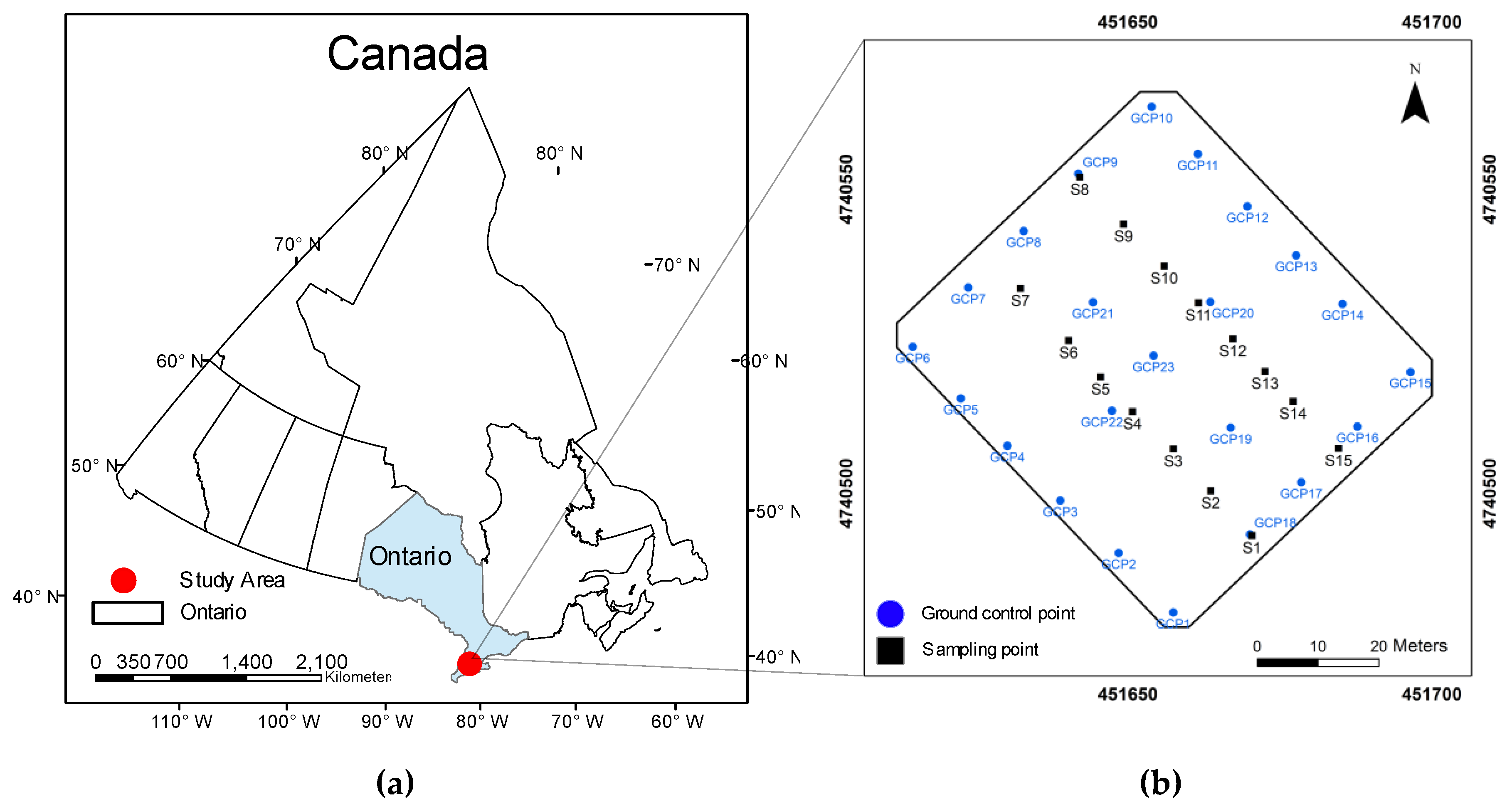
The study site is a winter wheat field located near Melbourne in southwest Ontario, Canada, which is shown as a red point in Figure 1a. This region of southwest Ontario has a single harvest per year for crops, with a relatively short growing season from early April to October. The growing season for winter wheat starts from the previous October and continues until the end of June. In the study site, a 50 m by 50 m area was used to collect ground-based crop height measurements and UAV-based imagery. The winter wheat was planted in October 2015, and the row spacing was 18–20 cm. Fifteen sampling points were selected in the study area and are shown as black square points in Figure 1b. The samples were collected along the row of winter wheat which could minimize the damage to crops. The ground-based crop height measurements were conducted at each sampling point, and the UAV flight was performed directly after the ground-based measurements. At each sampling point, three crop height measurements were collected within a 2-m area, and the average height was used to represent the canopy height in this study. In addition, 23 ground control points (GCPs) were set up in the field using white and black target boards for the entire growing season. The points were used as tie points for the images and multi-temporal UAV-based point cloud datasets during the point cloud generation in UAV images processing software to increase the relative accuracy of the dataset. They are shown as blue points in Figure 1b.
2.2. Remote Sensing Data Acquisition and Preprocessing
Multitemporal UAV-based imagery was collected using a DJI Phantom 3 UAV system with a high-resolution digital red, green, and blue (RGB) camera (DJI Technology Co., Ltd., Shenzhen, China). The multitemporal 3D point cloud datasets were generated from UAV-based imagery using Pix4Dmapper Pro (Pix4D) v2.4 (Pix4D SA, Lausanne, Switzerland) [48]. The output of the UAV-based 3D point cloud dataset has a similar format to LiDAR data but has a lower cost. Three UAV acquisitions at different crop growth stages were carried out on the winter wheat field on 16 May, 31 May, and 9 June 2016. The phenology of winter wheat represent by BBCH-scale are 31, 65, and 83, which are early, middle, and late stages, respectively [49]. These phenological stages were chosen for this study to evaluate the method using different crop heights.
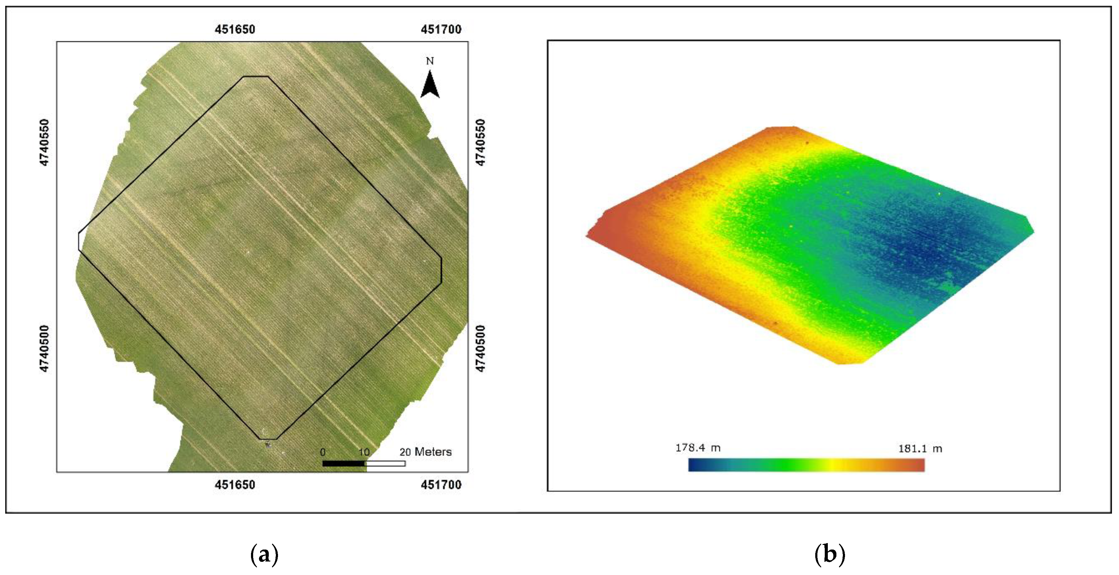
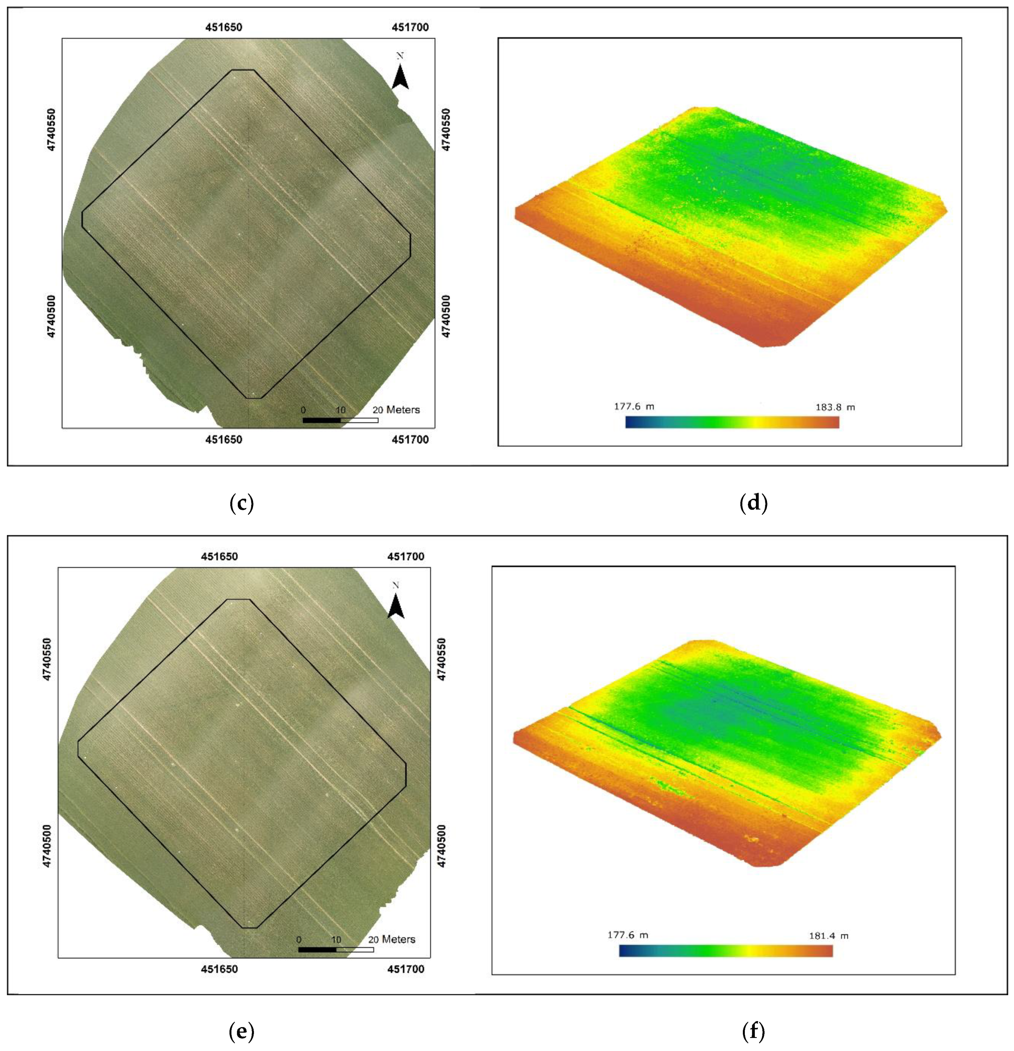
All UAV images in this study were captured in the nadir position. The flight height was 30 m above the ground, and the overlapping of all images was 90% on all sides to help the point cloud generation for farm field. The spatial resolution for all three aerial images is 1.5 cm. The UAV flight dates, number of images, points in the dataset, point density, average ground measurements, and crop phenology were listed in Table 1. The images were processed using Pix4D software to generate orthomosaic aerial images and 3D point cloud datasets. The ground control points were used in the processing of the orthomosaic aerial images and point cloud generation in Pix4D. The preprocessing of the output point cloud data, including data clipping and data format conversion, was conducted in C++ with the point cloud library. The orthomosaic images and the elevation of corresponding point cloud datasets in perspective view are shown in Figure 2.
2.3. Data Analysis
2.3.1. UAV-Based Point Cloud Distribution over Crop Fields
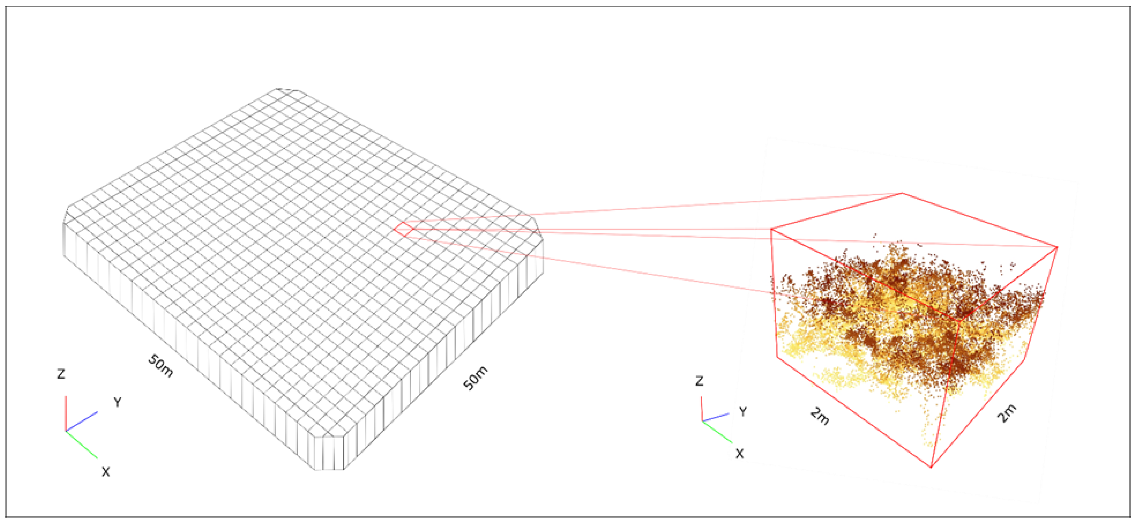
We divided the point cloud dataset into many 3D square cross-section columns with a ground area of 2 m by 2 m, as shown in Figure 3. After dividing the point cloud dataset into many 3D columns, the Otsu’s method was used to classify the points within each column into two groups; one was bare ground points and one was plant points [50]. The UAV-based 3D point cloud data for crop fields at different stages provided different distribution histograms in each column. At different growth stages of winter wheat in this study, the histogram can be divided into seven classes that represent different crop phenology stages, as shown in Figure 4.
In Figure 4, the brown bars represent the histogram of the bare ground points, and the green bars represent the histogram of the plant points in each column. Before the crop emergence, the points in each column are contributed by the bare ground (Figure 4a). The distribution of bare ground points showed that the estimated elevations of bare ground points have a variation of about 20 cm. This variation may be caused by the homogenization of the surface, which resulted in an inaccurate estimation of point position during the generation of the point cloud. After the crop emergence, a plant point histogram appears but shows the same range of elevation as the bare ground points (Figure 4b,c). As the crop grows, the histogram of plant points separates into two peaks, one made by points at the plant bottom; one made by points at the canopy. As the crop continues to grow taller, the number of points contributed by a crop will gradually increase, then the two peaks also become more apparent, and the distance between them increases (Figure 4d,e). The overall histogram has two general peaks. The number of bare ground points decreases. With the crop growth, the number of crop points will increase until the crop has a full canopy, and the first peak made by plant and bare ground points will gradually disappear in the histogram (Figure 4e,f). Finally, the histogram has only one peak, which is contributed by the crop canopy points (Figure 4g).
2.3.2. The Moving Cuboid Filter
The 3D point cloud dataset was first divided into many 2 m by 2 m 3D columns. These grid dimensions provided enough variability for intra-field monitoring in the crop field since the data collection resolution is 3 m for most farmers in our study area. The moving cuboid filter was applied in each column that satisfied two criteria at the same time: (1) close to the point cloud dataset within a specific vertical distance; (2) have enough neighboring points within a certain 3D cuboid.
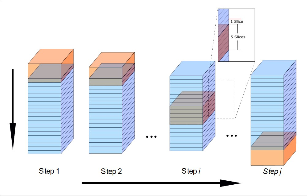
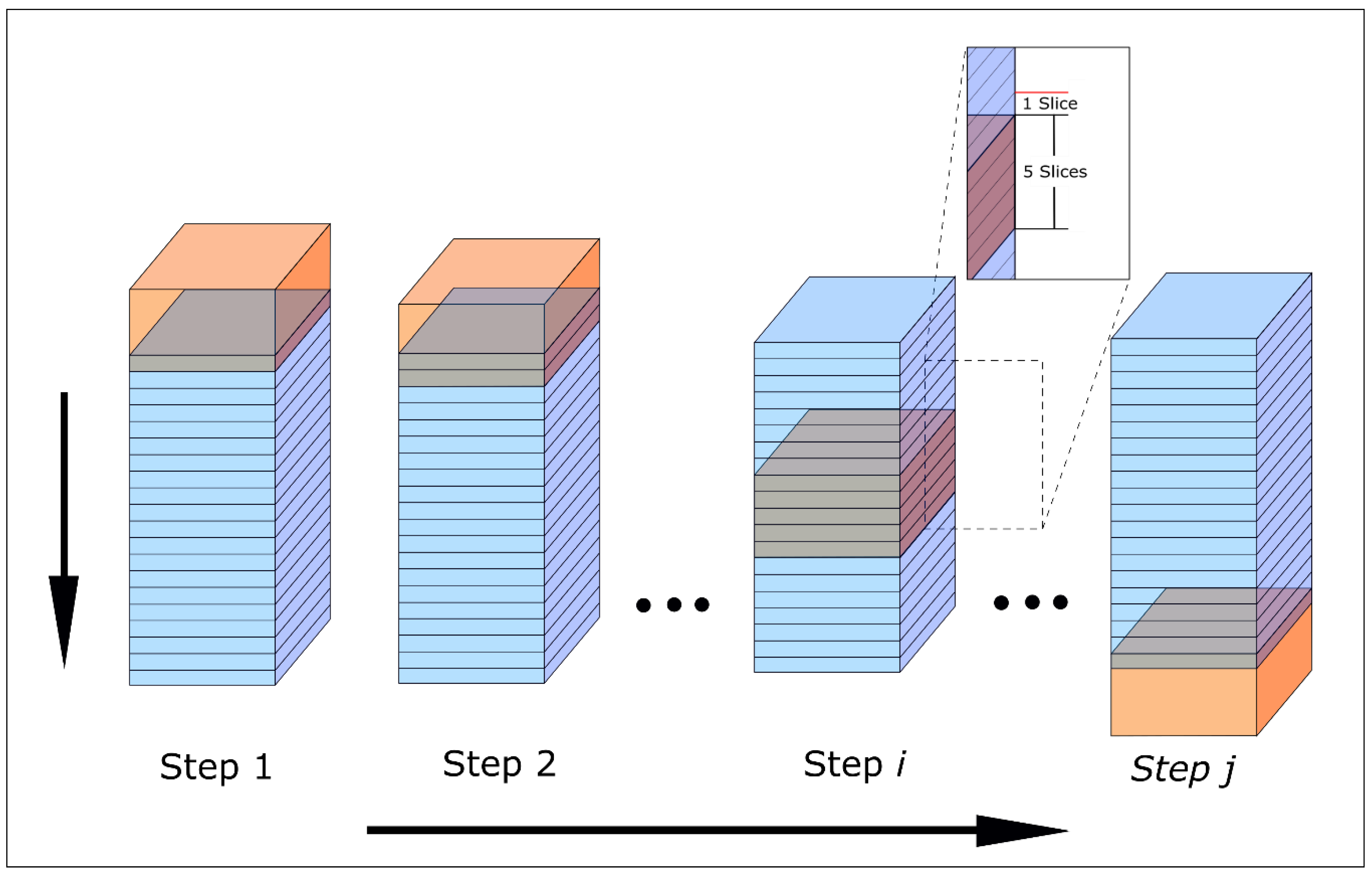
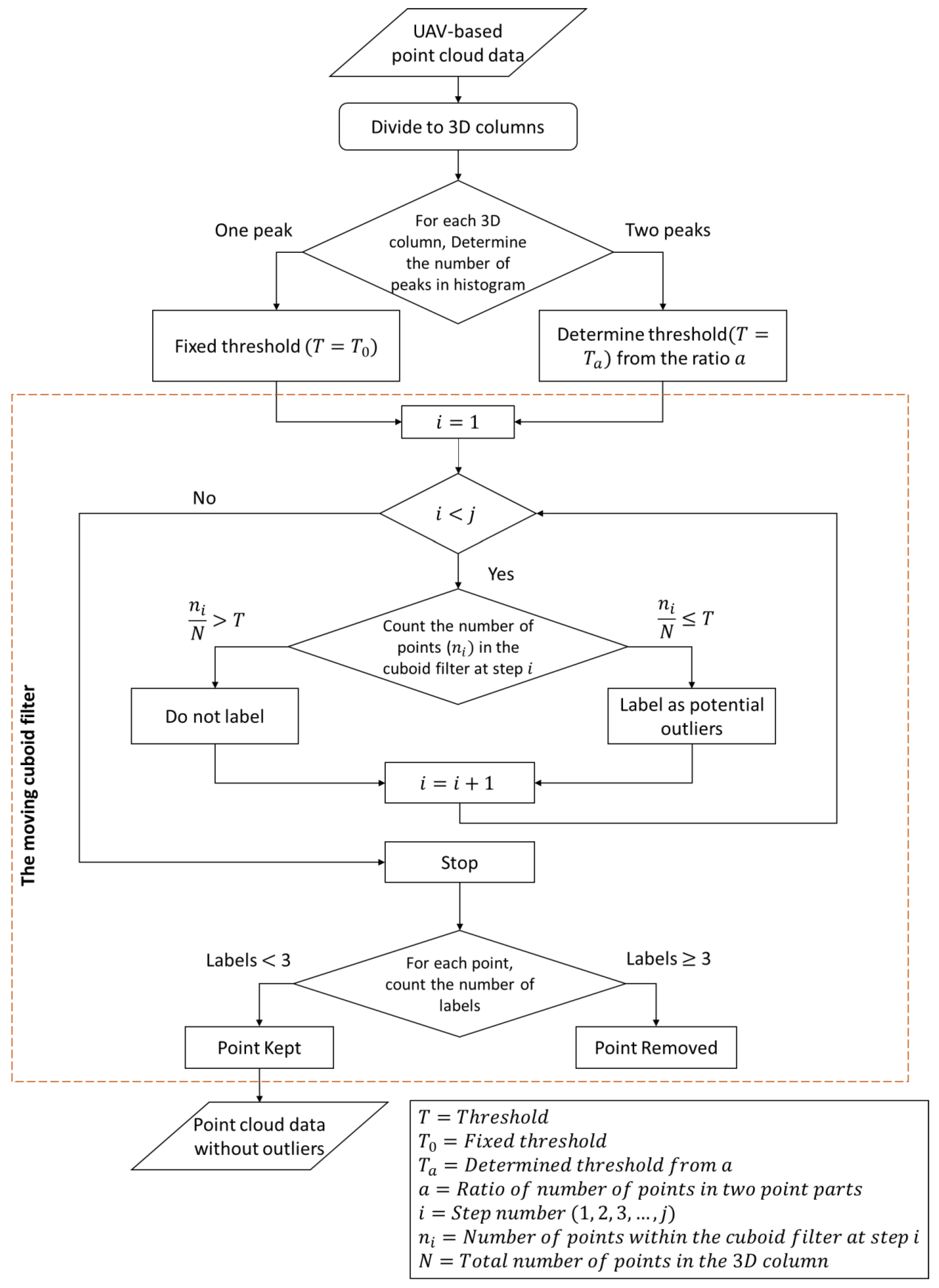
The moving cuboid filter is shown in Figure 5. First, the 3D column (blue cuboid) which is one voxel in the entire point cloud data is divided into many same thickness slices (1 cm thick). A moving orange cuboid filter includes five slices which moves down from the top of the column to the bottom in the z-direction, with a step of one slice. If the number of points in the moving cuboid filter is less than the threshold, all points within the cuboid filter are labeled as potential outliers. The cuboid filter contains five slices, and it moves down one slice in each step, so each point is labeled five times. Any point that has been labeled as a potential outlier more than half of the number of slices in the cuboid filter is considered an outlier and is trimmed from the column because the point is far from the point cloud datasets and has fewer neighboring points. In this study, the size of the moving cuboid filter was 2 m × 2 m × 5 cm and the moving step was 1 cm. The flow chart of the outlier filter is shown in Figure 6.
After eliminating the outliers using this moving cuboid filter and thresholds, the clean single 3D column will be divided into many sub-columns at the size of 0.5 m by 0.5 m. Since the size of the 3D column is 2 m by 2 m, the number of sub-columns is 16 in each column. After dividing the 3D column into sub-columns, the highest and lowest points in each sub-column will be used to calculate the height of wheat canopy height. Then, all 16 sub-columns heights will be used to calculate the average canopy height for one single 3D column to avoid the appearance of extreme results and make the height estimation more reliable.
2.3.3. Threshold Determination
The total number and the distribution of the point in a 3D column will affect the number of points in the cuboid filter at each step during the downward moving of the cuboid filter. The threshold of the moving cuboid filter is the ratio of the number of points at each step and the total number of points in the 3D column. This ratio ensures the threshold will not change with the variation of the total number of points in the 3D column and is affected by the point cloud distribution only.
According to Figure 4, the number of peaks will classify the histogram into two categories, one has one peak, and one has two peaks. When the histogram of point distribution has two peaks, the height value of the local minimum can be determined. The point cloud data will be separated into two parts: points have higher height value than the height of the local minimum in the histogram belong to high part and points have lower height value is a low part. The number of points in the high and low parts corresponds to and . The ratio is defined as:
When the histogram of point distribution has one peak, the value of is which is a special case in estimation. Therefore, a fixed threshold will be adopted for the 3D column with one peak in the histogram, which is . A changing threshold will be adopted for the 3D column with two peaks in the histogram. will be determined based on the value of . Since this study has the limited sampling points, the range of is used determine and the entire range of is divided into multiple intervals, and represent the interval nodes. The fixed values , , … will be adopted for based on the different intervals of .
Therefore, the threshold of the moving cuboid filter will be written as:
One peak:
Two peaks:
An evaluation test will be performed on each of the 3D columns at the 15 sampling points in the winter wheat field on 16 May and 31 May to determine the acceptable range of the threshold where the relative difference between the estimated and measured crop heights was less than 10%. First, the histograms of all these 3D columns will be normalized to the same scale. Savitzky–Golay filtering will be applied to smooth each histogram and determine the number of peaks and the value of the local minimum in the histogram. The value of will be calculated after determining the local minimum. Next, the estimated crop height was determined at thresholds from 0.1% to 10% of the points in the 3D column, and the step was 0.1%. The relationship between and will be determined.
2.3.4. Method Assessment
The ratio of the number of unsolved pixels and the total pixels in the study area will be calculated for all three winter wheat growth stages to verify the correctness of the moving cuboid filter. One pixel had an unacceptable estimation of crop height after applying the moving cuboid filter wad defined as an unsolved pixel. The canopy height for winter wheat at the same growing stage within a field should be similar. If any pixel has canopy height estimation much higher or lower than the average canopy height measured in the field, this pixel should be considered as an unsolved pixel. Hence, the absolute difference between the estimated height using the moving cuboid method and the average ground measurement was set to 20 cm in this study.
The Root Mean Square Error (RMSE) will be applied to evaluate the prediction errors in this study. In addition, the Mean Absolute Error (MAE) will be used to evaluate the average magnitude of the error of predicted canopy height. The RMSE and MAE will be calculated from predicted and ground measured canopy height on each measurement date, and the overall RMSE and MAE will be calculated for all three dates together to evaluate the accuracy of the moving cuboid filter in canopy height estimation.
For further validation, a comparison will be performed based on the RMSE, MAE, average height, standard deviation, and unsolved pixel rate between the estimated canopy height via both the Khanna’s method and the moving cuboid filter and ground measurements. Khanna’s method firstly divided the point cloud dataset into many columns, which are 3D grid cells with the same area. Then the Otus’s method was used to determine the threshold and classify the points into ground and vegetation parts. The fixed threshold 1% will be only applied on vegetation part to remove the top 1% of the vegetation points. The final canopy height was calculated from the highest and lowest points of the rest of the vegetation points in the column.
3. Results
3.1. Threshold T and Range of α for Winter Wheat
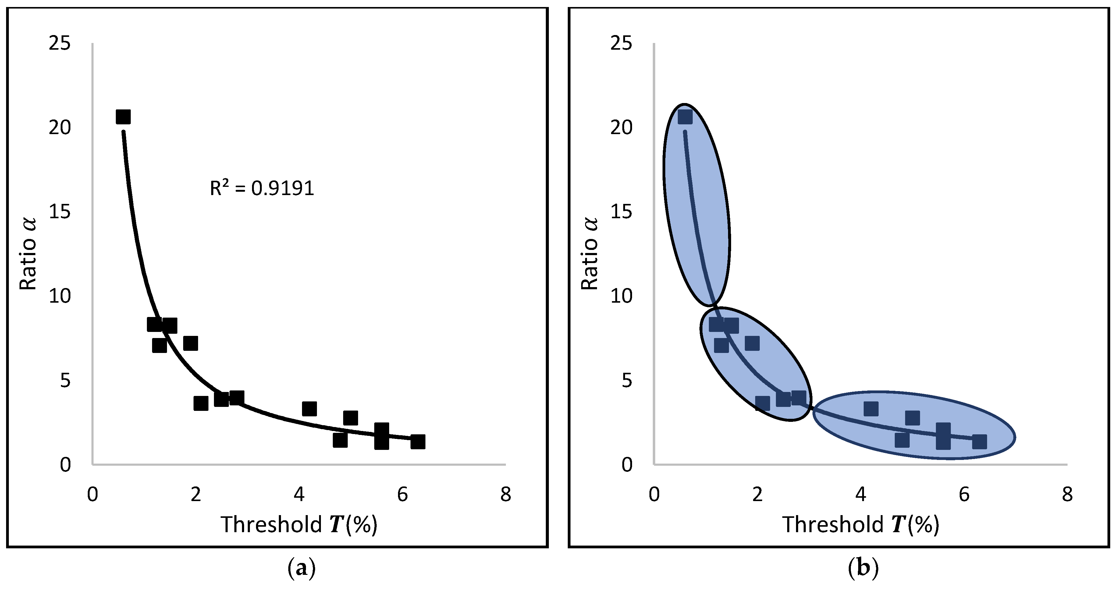
After evaluating the value of threshold at all sampling points on 16 May and 31 May, we found that when the histogram of point in the 3D column had one peak (Figure 4a–c), the acceptable range of threshold was from 0.1% to 0.2%. Therefore, we adopted a fixed threshold of = 0.1%. When the histogram of point in the 3D column had two peaks, the acceptable range of threshold changes with . The mean of the upper bound and the lower bound of the range is adopted as . The relationship between and is shown in Figure 7. is highly correlated with (R2 = 0.9191), and the data of and shows in Table 2. Since the histograms of point cloud distribution on 16 May all had one peak, and on 31 May had two peaks, the fixed threshold was determined from all sampling points on 16 May, and the changing threshold was determined based on the value of from all sampling point on 31 May. As the power regression was applied for and , the distribution was classified into the three groups in this study, shown in Figure 7b. Two classes are concentrated at the tail parts of the curve and one class was concentrated at the middle part of this curve. The nodes of the range of were determined that . The was adopted for this experiment is:
3.2. Canopy Height Estimation at Different Growth Stages Using the Moving Cuboid Filter
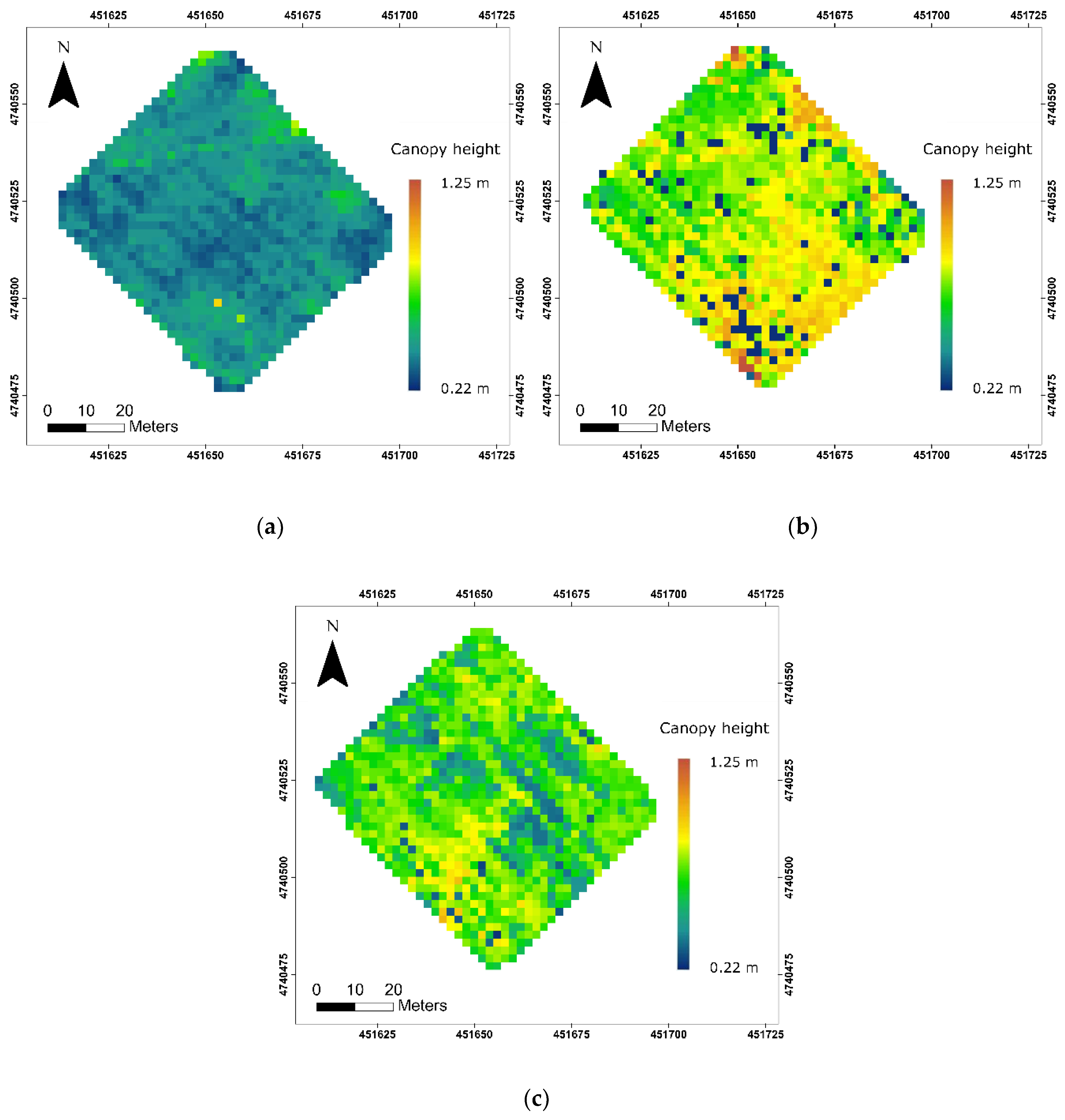
To show the variation of this moving cuboid filter at different wheat growth stages, three raw maps of the wheat canopy height at different stages are shown in Figure 8.
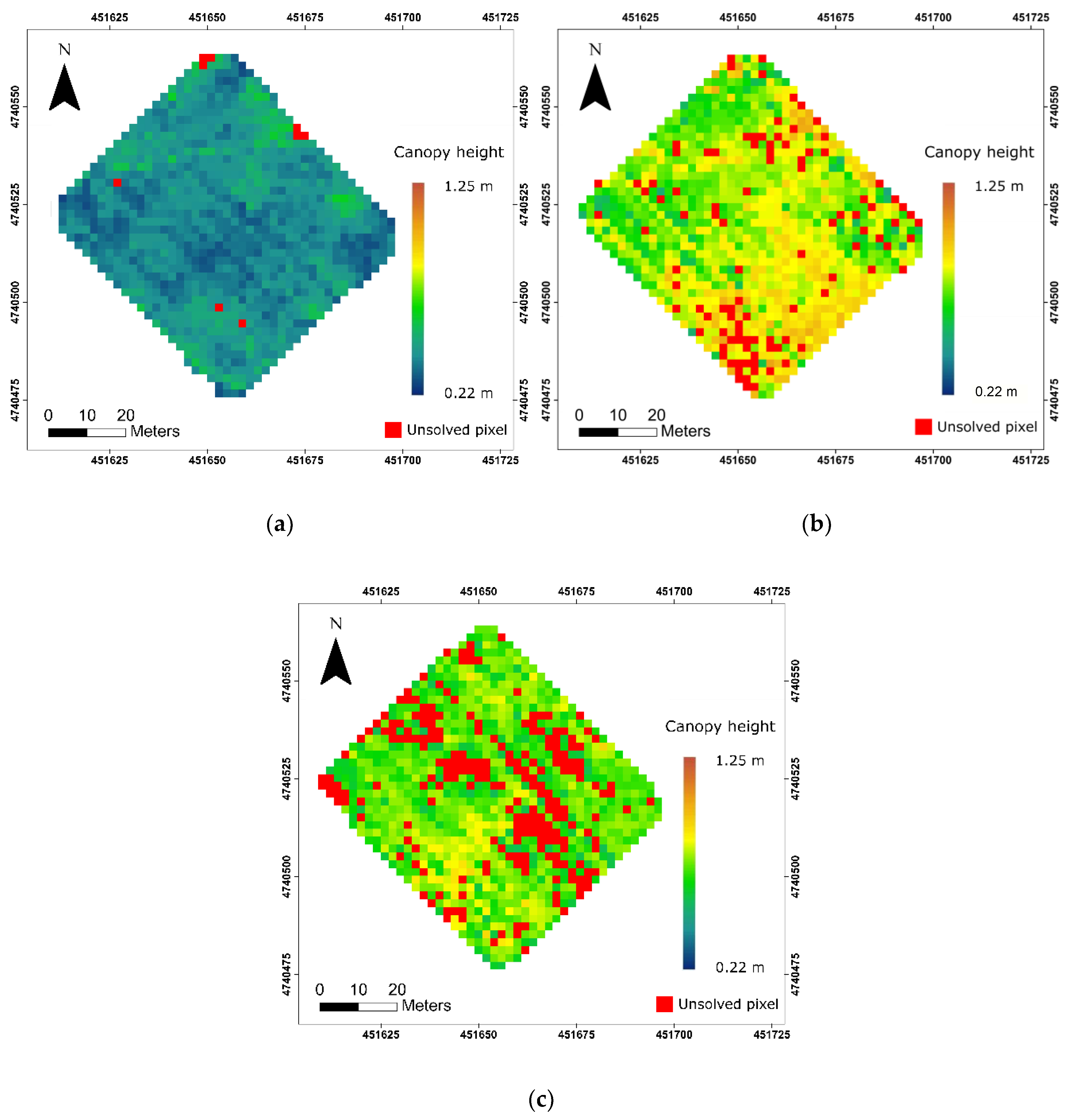
The average canopy height was the average of all ground height measurements in each date, which were 42.3 cm, 73.7 cm, and 74.3 cm for 16 May, 31 May, and 9 June. If the absolute difference of the estimated canopy height in the pixel and the average ground measurements is greater than 20 cm, this canopy height of the pixel was considered a failure estimation, as shown in Figure 9. The unsolved pixel rate was 0.8%, 8.3%, and 21.7% on 16 May, 31 May, and 9 June, respectively.
3.3. Canopy Height Maps after Interpolating for Unsolved Pixels
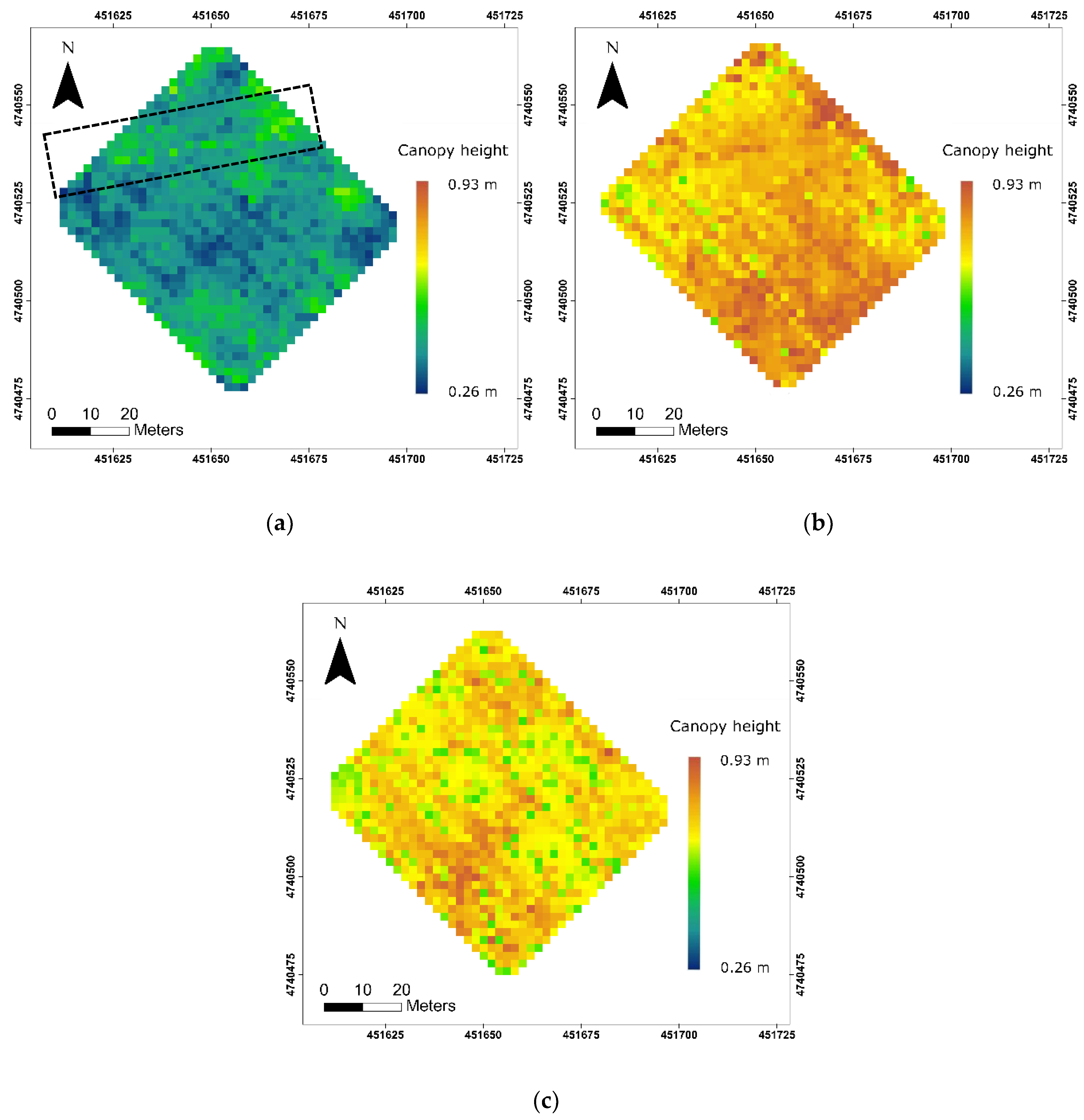
After removing the unsolved pixels in the map, the canopy height of the rest of the unsolved pixels was recalculated using the inverse distance weighted (IDW) algorithm based on the neighboring points. The final canopy height maps at different growing stages are shown in Figure 10.
The average canopy height was 40.1 cm on 16 May, and the standard deviation was 0.06; the average canopy height was 76.7 cm with a standard deviation of 0.07 on 31 May; the average canopy height was 70.3 cm with a standard deviation of 0.06 on 9 June. To show the accuracy of the moving cuboid filter, the RMSE and MAE between the estimated and ground-measured canopy heights for 15 sampling points at all growing stages were compared. The RMSE was 6.5 cm on 16 May, 4.5 cm on 31 May, and 7.7 cm on 9 June; the overall RMSE was 6.37 cm. The MAE was 5.1 cm on 16 May, 3.8 cm on 31 May, and 6.4 cm on 9 June; the overall MAE was 5.07 cm.
In the northern part of the study area, one row of winter wheat had higher plant height estimations than the rest of the study area. This row is a vehicle trail made in the winter season before the wheat emergence which is within the black dash rectangle in Figure 10a. The trail could be clearly observed on the maps of canopy height on 16 May and 31 May, but not on 9 June. The same observation can be made from the aerial images on 16 May, 31 May, and 9 June (Figure 2); the trail gradually fades over time.
3.4. Canopy Height Results Using the Point Statistical Method Developed by Khanna
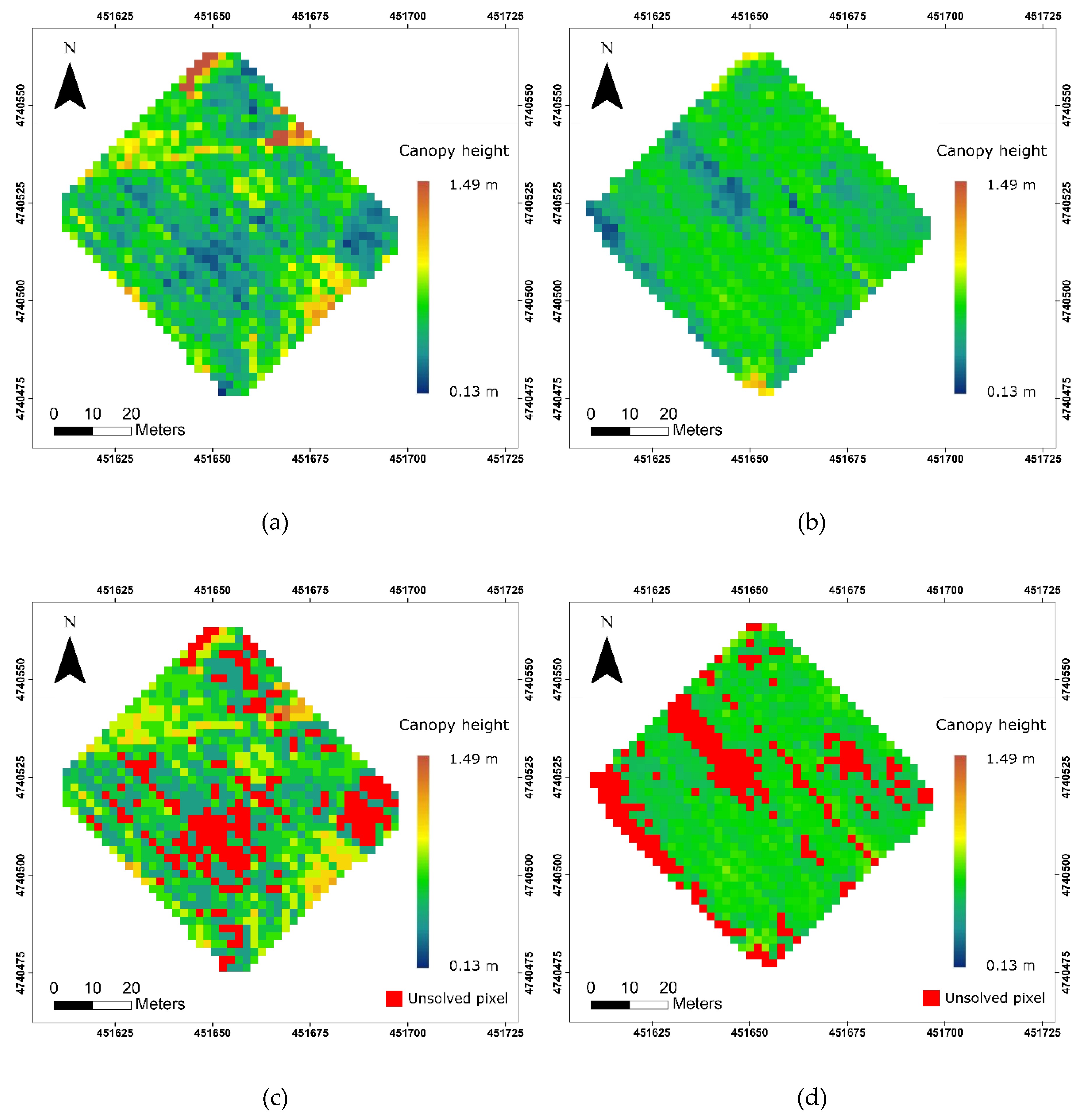
The results generated from another statistical method developed by Khanna et al. [30] are shown in Figure 11. The method developed in this study does not perform well in canopy height estimation on 9 June, and Khanna’s method is designed for early wheat stage height estimation, so the 16 May and 31 May results were compared in this study.
The average height of the winter wheat canopy estimated using Khanna’s method was 26 cm on 16 May and 60.25 cm on 31 May. The standard deviation was 11.33 and 12.26 on 16 May and 31 May, respectively. The RMSE was 17.03 cm on 16 May and 9.03 cm 31 May. The MAE was 15.5 cm on 16 May and 7.51 cm on 31 May. The unsolved pixel rates were 19.4% and 21.1% on 16 May and 31 May, respectively. A comparison of the moving cuboid filter and Khanna methods is shown in Table 3.
4. Discussion
4.1. Advantages of the Moving Cuboid Filter
The canopy height estimation from the UAV-based point cloud data uses the spatial structure information on image points so a commercial digital camera can be used for image acquisition rather than an expensive multispectral or hyperspectral camera. In addition, the point cloud data contains color information on each point [38]. Currently, many studies used crop height model (CHM) to retrieve crop and forest canopy height from the calculation between DTM and DSM. The CHM methods could achieve crop height estimation for the entire growing season; however, the complexity of ground control points collection must be considered for multiple times data collection. As compared with the CHM model, the moving cuboid filter presented in this study reduced the workload in the field to one UAV data collection. In addition, ground control points acquisition does not require high-accuracy RTK-GNSS since the ground control points in this study are used to align adjacent images and multi-date datasets. These advantages of the moving cuboid filter enable simple UAV operation in the field for crop height monitoring.
In this study, the moving cuboid filter method is tested at three winter wheat growth stages and it is used to estimate the canopy heights with a fixed threshold or a changing threshold . The moving cuboid filter performed better than the Khanna’s simple fixed threshold filter on wheat canopy height estimation at these three growing stages in terms of estimation range, RMSE and MAE, and unsolved pixel rate. According to the results derived from the above tests, a changing threshold with a moving cuboid filter was more adaptable to different point distribution due to the canopy changes in different growing stages than a fixed threshold filter. To remove outliers from crop point cloud data, the moving cuboid filter did not only consider the relationship between point and its neighboring points but also concerned about the continuity of points in the vertical direction. The thresholds determined from the point distribution in each voxel were different. Compared with studies that adopt a simple fixed threshold or practical value, the moving cuboid filter had better performance on crop outlier removal at different growing stages which may reduce human error.
4.2. Limitations and Uncertainties of the Moving Cuboid Filter
In this study, the number of peaks was determined from the histogram of the point cloud data distribution in each column before applying the moving cuboid filter. According to Figure 4a–c, the bare ground and the crop at phenology of BBCH 31 has only one peak in the histogram of point distribution. From the observation of the distribution of bare ground points in October of the previous year, it can be found that the bare ground points presented a variation in the estimation of evaluation. This issue will affect the crop height estimation in early plant developing stages when the crop height is low, such as early leaf development and tillering stages [31]. This method performed well on the canopy height estimation of wheat at the phenology of BBCH 31. A fixed threshold of 0.1% was adopted in this study rather than a fixed threshold of 1% of plant points in Khanna’s method. The reason that different thresholds are selected is that the total numbers and densities of points in these two studies are different. The threshold may change due to the different data collection methods and types of crops; hence it will need to be determined in different cases. According to Figure 4d,e, most of the columns have two peaks in the histograms of point distributions on 31 May. For this reason, the threshold was established based on all sampling points from the dataset on 31 May. A regression model between and was established in this study to be used to determine the threshold from the calculation of . However, this inversion method could introduce thresholds out of the acceptable range of thresholds and result in incorrect canopy height estimation. Therefore, instead of calculating from the inversion of the regression model, three values were adopted based on three intervals of the range of in this study. Since the sampling points were limited in this winter wheat dataset and only three intervals of the range of α and were classified in this study, the unsolved pixels were still present in the results. Increase of the sampling points could help to narrow the interval of the range of and and improve the accuracy of crop height estimation in the future study.
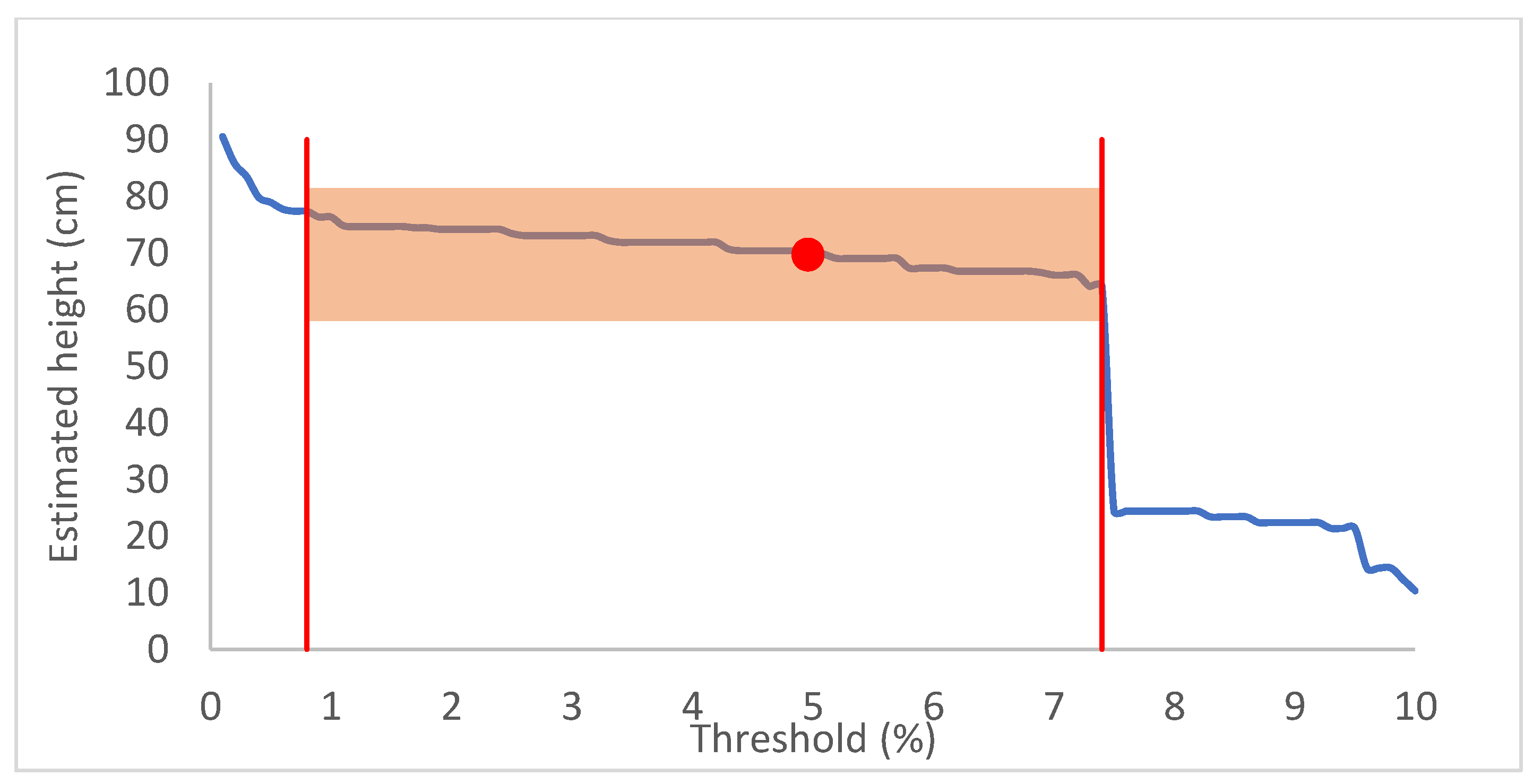
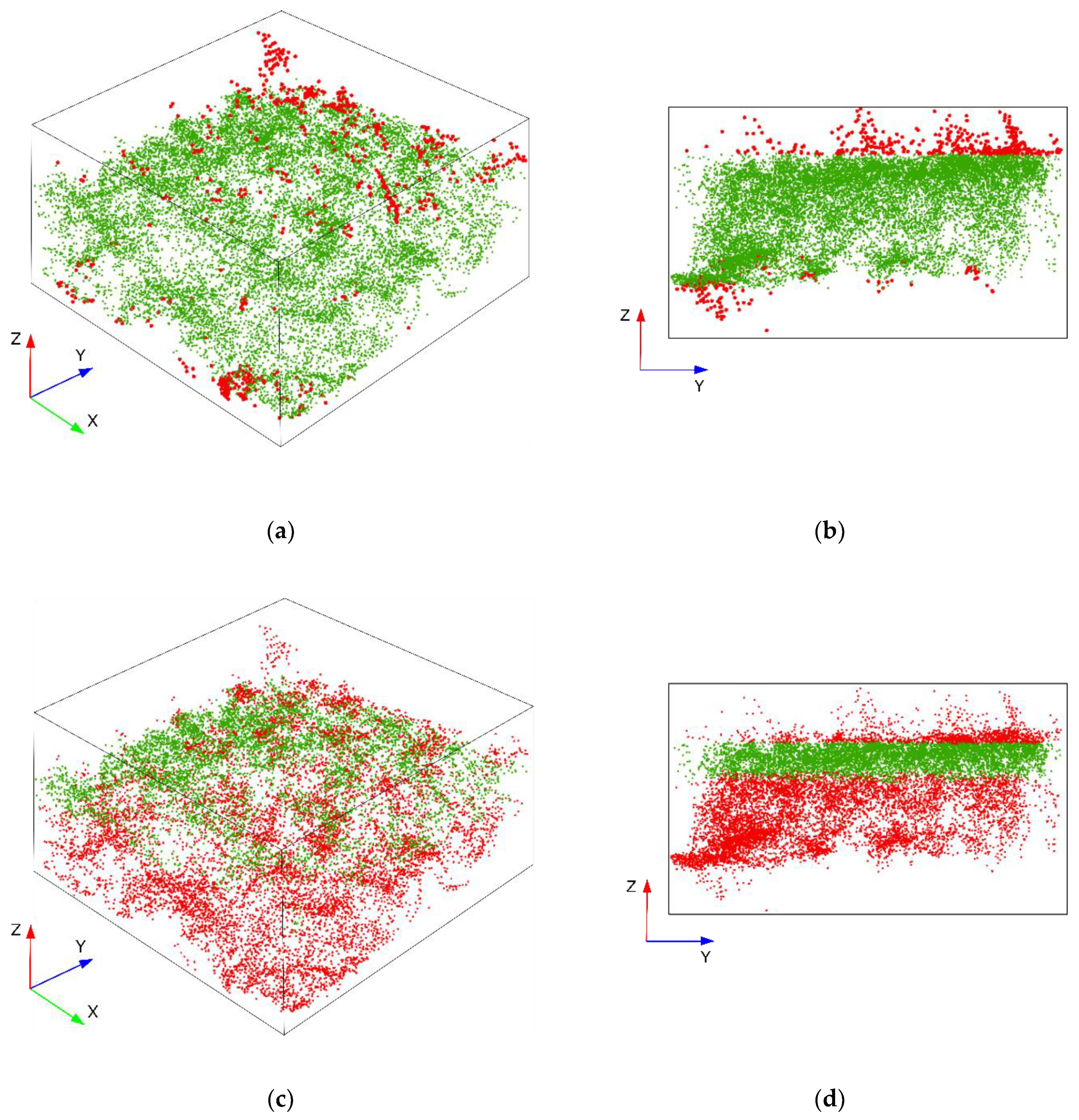
After evaluating the acceptable range of the threshold , we found that the estimated crop canopy height in each column reduces as the threshold increases. Due to the human error of in-situ crop height measurements, the threshold is an acceptable range instead of an optimal value. In this study, the acceptable range of threshold for the 3D column with one peak in its histogram of point distribution ranged from 0.1% to 0.2%. Therefore, it was easy to determine . However, the acceptable range of threshold for the 3D column with two peaks varies greatly. For example, the changes in the estimated canopy height and threshold selections from 0.1% to 10% of the total number of points in the column of sample point eight on 31 May are shown in Figure 12. The ground-measured canopy height was 69.7 cm in this column. When the absolute difference from the ground-measured and the estimated canopy height is less than 10%, the corresponding threshold range is the acceptable range of thresholds. In this case, within the acceptable range of thresholds from 0.9% to 7.4%, the estimated canopy height was 64.1 cm to 76.3 cm, and the optimal estimated canopy height is 70.38 cm at the 5% threshold. However, according to Figure 12, the estimated canopy height suddenly reduced more than 40 cm when the threshold exceeded 7.4%. Figure 13 shows the result of threshold selection in this column trimmed using the moving cuboid filter at different thresholds 7.4% (Figure 13a,b) and 7.5% (Figure 13c,d). The trimmed outliers are shown as red points in Figure 13. If the selection of threshold is out of the acceptable range of thresholds, the overestimates and underestimates could affect the final canopy height estimation. This is one of the sources of the unsuccessful estimations of canopy height and unsolved pixel on 31 May data.
The number of unsolved pixels significantly increased from 31 May to 9 June. In addition to the issue of selecting a threshold that was out of the affectable threshold range, the primary source of unsolved pixels was from the dataset itself on 9 June. The growing stage of the winter wheat on 9 June was the ripening stage (BBCH is 83), corresponding to complete heading and starting fruiting. At this stage, the winter wheat should have an almost complete canopy, and the histogram of point distributions in all columns should be close to the histogram in Figure 4f,g. In the case of Figure 4g, the point cloud dataset may only contain the points of the top canopy and no bare ground points because the camera is unable to penetrate the crop canopy and capture soil images from any observation angle. Due to the missing bare ground information, part of the canopy height on 9 June was estimated lower than that on 31 May, which can be observed from canopy height map on 31 May and 9 June (Figure 10). This shows that the moving cuboid filter had difficulty estimating the winter wheat canopy height after the full canopy stages.
4.3. Applications of the Moving Cuboid Filter
Although the proposed method is challenging when estimating canopy height after the full canopy emerges, the average height does not change significantly after the heading stages in winter wheat. In this study, this method achieved the canopy height estimation between the stem extension and heading stages. These stages are essential in winter wheat monitoring. The information from these stages can be used in biomass and final yield estimation [19]. Since this method enables a simple operation of UAV in the field, it could be an effective method that can be widely used to help end-user to monitor their crops and support real-time decision making for farm management.
The proposed moving cuboid filter uses both the bare ground and plant canopy point in the point cloud dataset to estimate winter wheat canopy height. Although the structure of wheat canopy is complicated due to the different row distance, variable crop heights, and different sizes of leaves and stems, the point cloud data can still provide the information of both bare ground and plant points before the wheat has a full canopy. This method could be applied to other crops with simple canopy structure and less density, such as corn and tobacco, but the parameter of moving cuboid filter and thresholds may need to be adjusted accordingly. To implement this method on other crops, the UAV system should keep at a relatively low flight altitude, and a high-resolution camera will help to collect fine resolution images.
5. Conclusions
The applied moving cuboid filter provides a suitable method for eliminating noise from UAV-based 3D point cloud datasets for winter wheat fields. First, this moving cuboid filter considers the density of points in a horizontal direction. A fixed threshold is used for outlier removal in the early stage of winter wheat. A changing threshold is used for outlier removal in the later stages of winter wheat. According to the range of , the changing threshold is selected based on the different histograms of point distribution. In addition to the horizontal direction, the moving cuboid filter also considers the continuation of points in a vertical direction. After labeling all points in the 3D column, points with more labels are trimmed as outliers. The filter has stable performance in canopy height estimation before the winter wheat has a full canopy and lower RMSE and MAE than ground measurements. Although this method has a relatively higher RMSE at early growth stages and a lower accuracy at the full canopy stage, it provides a canopy height monitoring window for winter wheat from the beginning of the stem extension stage to the end of the heading stage (BBCH 31 to 65). The accuracy of this method decreases as the winter wheat grew.
This method provides a potential direction for crop height estimation using UAV-based 3D point cloud data, which could help farmers easily monitor farm fields and quickly obtain real-time crop height information. Future canopy height studies using UAV-based 3D point cloud data should focus on the estimation of to resolve the issue of unsolved pixels. A larger field area and more ground sampling points might provide useful information for selection. In addition, more parameter adjustment studies such as height extraction from low-density point cloud datasets and final map generation with lower resolutions should be conducted to reduce processing time. The moving cuboid filter could also be evaluated for different crop types such as corn and soybean in future studies.
Author Contributions
Y.S. contributed to the design and implementation of the proposed methodology and wrote and revised the paper; J.W. contributed to the discussion of the results and revised the paper.
Funding
This work is partially funded by an NSERC discovering Grant awarded to Wang, a MITACS accelerate internship sponsored by MITACS and A&L Canada Laboratories Inc., and the Canadian Space Agency SOAR-E program (Grant No. SOAR-E-5489).
Acknowledgments
We would like to thank Chunhua Liao, Zhenpei Li and Yuechen Li for their helpful work on field data collection.
Conflicts of Interest
The authors declare no conflict of interest.
References
- Freeman, P.K.; Freeland, R.S. Agricultural UAVs in the U.S.: Potential, policy, and hype. Remote Sens. Appl. Soc. Environ. 2015, 2, 35–43. [Google Scholar] [CrossRef]
- Primicerio, J.; Di Gennaro, S.F.; Fiorillo, E.; Genesio, L.; Lugato, E.; Matese, A.; Vaccari, F.P. A flexible unmanned aerial vehicle for precision agriculture. Precis. Agric. 2012, 13, 517–523. [Google Scholar] [CrossRef]
- Park, S.; Ryu, D.; Fuentes, S.; Chung, H.; Hern, E.; Connell, M.O. Adaptive Estimation of Crop Water Stress in Nectarine and Peach Orchards Using High-Resolution Imagery from an Unmanned Aerial Vehicle (UAV). Remote Sens. 2017, 9, 828. [Google Scholar] [CrossRef]
- Swain, K.C.; Thomson, S.J.; Jayasurya, H.P.W. Adoption of an unmanned helicopter for low-altitude remote sensing to estimate yield and total biomass of a rice crop. Trans. ASAE 2010, 53, 21–27. [Google Scholar] [CrossRef]
- Lottes, P.; Khanna, R.; Pfeifer, J.; Siegwart, R.; Stachniss, C. UAV-Based Crop and Weed Classification for Smart Farming. Available online: http://www.ipb.uni-bonn.de/wp-content/papercite-data/pdf/lottes17icra.pdf (accessed on 24 May 2019).
- Zhang, C.; Kovacs, J.M. The application of small unmanned aerial systems for precision agriculture: A review. Precis. Agric. 2012, 13, 693–712. [Google Scholar] [CrossRef]
- Nebiker, S.; Annen, A.; Scherrer, M.; Oesch, D. A light-weight multispectral sensor for micro uav–opportunities for very high resolution airborne remote sensing. Int. Arch. Photogramm. Remote Sens. Spat. Inf. Sci. 2008, XXXVII, 1193–1200. [Google Scholar]
- Huang, J.; Wang, X.; Li, X.; Tian, H.; Pan, Z. Remotely Sensed Rice Yield Prediction Using Multi-Temporal NDVI Data Derived from NOAA’s-AVHRR. PLoS ONE 2013, 8, 1–13. [Google Scholar] [CrossRef] [PubMed]
- D’Oleire-Oltmanns, S.; Marzolff, I.; Peter, K.D.; Ries, J.B. Unmanned Aerial Vehicle (UAV) for Monitoring Soil Erosion in Morocco. Remote Sens. 2012, 4, 3390–3416. [Google Scholar] [CrossRef] [Green Version]
- Hunt, E.R.; Dean Hively, W.; Fujikawa, S.J.; Linden, D.S.; Daughtry, C.S.T.; McCarty, G.W. Acquisition of NIR-green-blue digital photographs from unmanned aircraft for crop monitoring. Remote Sens. 2010, 2, 290–305. [Google Scholar] [CrossRef]
- Kalisperakis, I.; Stentoumis, C.; Grammatikopoulos, L.; Karantzalos, K. Leaf Area Index Estimation in Vineyards From Uav Hyperspectral Data, 2D Image Mosaics and 3D Canopy Surface Models. ISPRS Int. Arch. Photogramm. Remote Sens. Spat. Inf. Sci. 2015, XL-1/W4, 299–303. [Google Scholar] [CrossRef]
- Hoffmann, H.; Jensen, R.; Thomsen, A.; Nieto, H.; Rasmussen, J.; Friborg, T. Crop water stress maps for entire growing seasons from visible and thermal UAV imagery. Biogeosciences 2016, 1–30. [Google Scholar] [CrossRef]
- Schirrmann, M.; Hamdorf, A.; Garz, A.; Ustyuzhanin, A.; Dammer, K. Estimating wheat biomass by combining image clustering with crop height. Comput. Electron. Agric. 2016, 121, 374–384. [Google Scholar] [CrossRef]
- Agüera, F.; Carvajal, F.; Pérez, M. Measuring Sunflower Nitrogen Status From an Unmanned Aerial Vehicle-Based System and an on the Ground Device. ISPRS Int. Arch. Photogramm. Remote Sens. Spat. Inf. Sci. 2012, XXXVIII-1/C22, 33–37. [Google Scholar] [CrossRef]
- Kolejka, J.; Plánka, L. Technical Report: The Development and Experience with UAV Research Applications in Former Czechoslovakia (1960s–1990s). Pure Appl. Geophys. 2018. [Google Scholar] [CrossRef]
- Yin, X.; Mcclure, M.A.; Jaja, N.; Tyler, D.D.; Hayes, R.M. In-Season Prediction of Corn Yield Using Plant Height under Major Production Systems. Agron. J. 2011, 103, 923–929. [Google Scholar] [CrossRef]
- Shaker, I.F.; Abd-Elrahman, A.; Abdel-Gawad, A.K.; Sherief, M.A. Building extraction from high resolution space images in high density residential areas in the Great Cairo region. Remote Sens. 2011, 3, 781–791. [Google Scholar] [CrossRef]
- Lagomasino, D.; Fatoyinbo, T.; Lee, S.K.; Simard, M. High-resolution forest canopy height estimation in an African blue carbon ecosystem. Remote Sens. Ecol. Conserv. 2015, 1, 51–60. [Google Scholar] [CrossRef]
- Li, W.; Niu, Z.; Chen, H.; Li, D.; Wu, M.; Zhao, W. Remote estimation of canopy height and aboveground biomass of maize using high-resolution stereo images from a low-cost unmanned aerial vehicle system. Ecol. Indic. 2016, 67, 637–648. [Google Scholar] [CrossRef]
- Zhang, L.; Grift, T.E. A LIDAR-based crop height measurement system for Miscanthus giganteus. Comput. Electron. Agric. 2012, 85, 70–76. [Google Scholar] [CrossRef]
- Hoffmeister, D.; Waldhoff, G.; Korres, W.; Curdt, C.; Bareth, G. Crop height variability detection in a single field by multi-temporal terrestrial laser scanning. Precis. Agric. 2016, 17, 296–312. [Google Scholar] [CrossRef]
- Hämmerle, M.; Höfle, B. Direct derivation of maize plant and crop height from low-cost time-of-flight camera measurements. Plant Methods 2016, 1–13. [Google Scholar] [CrossRef]
- Dal Mutto, C.; Zanuttigh, P.; Cortelazzo, G.M. Time-of-Flight Cameras and Microsoft KinectTM; Springer Briefs in Electrical and Computer Engineering; Springer: Boston, MA, USA, 2012; ISBN 978-1-4614-3806-9. [Google Scholar]
- Ryan, J.C.; Hubbard, A.L.; Box, J.E.; Todd, J.; Christoffersen, P.; Carr, J.R.; Holt, T.O.; Snooke, N. UAV photogrammetry and structure from motion to assess calving dynamics at Store Glacier, a large outlet draining the Greenland ice sheet. Cryosphere 2015, 9, 1–11. [Google Scholar] [CrossRef] [Green Version]
- Smith, M.W.; Carrivick, J.L.; Quincey, D.J. Structure from motion photogrammetry in physical geography. Prog. Phys. Geogr. 2015, 40, 247–275. [Google Scholar] [CrossRef]
- Carrivick, J.L.; Smith, M.W.; Quincey, D.J. Structure from Motion in the Geosciences; John Wiley & Sons, Ltd.: Chichester, UK, 2016; ISBN 1118895827. [Google Scholar]
- Mlambo, R.; Woodhouse, I.H.; Gerard, F.; Anderson, K. Structure from motion (SfM) photogrammetry with drone data: A low cost method for monitoring greenhouse gas emissions from forests in developing countries. Forests 2017, 8, 68. [Google Scholar] [CrossRef]
- Harwin, S.; Lucieer, A. An Accuracy Assessment of Georeferenced Point Clouds Produced Via Multi-View Stereo Techniques Applied To Imagery Acquired Via Unmanned Aerial Vehicle. ISPRS Int. Arch. Photogramm. Remote Sens. Spat. Inf. Sci. 2012, XXXIX-B7, 475–480. [Google Scholar] [CrossRef]
- Westoby, M.J.; Brasington, J.; Glasser, N.F.; Hambrey, M.J.; Reynolds, J.M. ‘Structure-from-Motion’ photogrammetry: A low-cost, effective tool for geoscience applications Introduction. Geomorphology 2012, 179, 300–314. [Google Scholar] [CrossRef]
- Khanna, R.; Martin, M.; Pfeifer, J.; Liebisch, F.; Walter, A.; Siegwart, R. Beyond Point Clouds—3D Mapping and Field Parameter Measurements using UAVs. In Proceedings of the IEEE 20th Conference on Emerging Technologies & Factory Automation, Luxembourg City, Luxembourg, 8–11 September 2015; pp. 5–8. [Google Scholar]
- Grenzdörffer, G.J. Crop height determination with UAS point clouds. In Proceedings of the International Archives of the Photogrammetry, Remote Sensing and Spatial Information Sciences—ISPRS Archives, Denver, CO, USA, 17–20 November 2014; pp. 135–140. [Google Scholar]
- Anthony, D.; Elbaum, S.; Lorenz, A.; Detweiler, C. On crop height estimation with UAVs. IEEE Int. Conf. Intell. Robot. Syst. 2014, 4805–4812. [Google Scholar] [CrossRef] [Green Version]
- Bendig, J.; Bolten, A.; Bennertz, S.; Broscheit, J.; Eichfuss, S.; Bareth, G. Estimating biomass of barley using crop surface models (CSMs) derived from UAV-based RGB imaging. Remote Sens. 2014, 6, 10395–10412. [Google Scholar] [CrossRef]
- Brocks, S.; Bendig, J.; Bareth, G. Toward an automated low-cost three-dimensional crop surface monitoring system using oblique stereo imagery from consumer-grade smart cameras. J. Appl. Remote Sens. 2016, 10, 046021. [Google Scholar] [CrossRef] [Green Version]
- Ota, T.; Ogawa, M.; Shimizu, K.; Kajisa, T.; Mizoue, N.; Yoshida, S.; Takao, G.; Hirata, Y.; Furuya, N.; Sano, T.; et al. Aboveground Biomass Estimation Using Structure from Motion Approach with Aerial Photographs in a Seasonal Tropical Forest. Forests 2015, 6, 3882–3898. [Google Scholar] [CrossRef] [Green Version]
- Gil-Docampo, M.L.; Arza-García, M.; Ortiz-Sanz, J.; Martínez-Rodríguez, S.; Marcos-Robles, J.L.; Sánchez-Sastre, L.F. Above-ground biomass estimation of arable crops using UAV-based SfM photogrammetry. Geocarto. Int. 2019, 0, 1–13. [Google Scholar] [CrossRef]
- Chang, A.; Jung, J.; Maeda, M.M.; Landivar, J. Crop height monitoring with digital imagery from Unmanned Aerial System (UAS). Comput. Electron. Agric. 2017, 141, 232–237. [Google Scholar] [CrossRef]
- Chu, T.; Starek, M.J.; Brewer, M.J.; Murray, S.C.; Pruter, L.S. Characterizing canopy height with UAS structure-from-motion photogrammetry—Results analysis of a maize field trial with respect to multiple factors. Remote Sens. Lett. 2018, 9, 753–762. [Google Scholar] [CrossRef]
- Birdal, A.C.; Avdan, U.; Türk, T. Estimating tree heights with images from an unmanned aerial vehicle. Geomat. Nat. Hazards Risk 2017, 8, 1144–1156. [Google Scholar] [CrossRef] [Green Version]
- Wolff, K.; Kim, C.; Zimmer, H.; Schroers, C.; Botsch, M.; Sorkine-Hornung, O.; Sorkine-Hornung, A. Point Cloud Noise and Outlier Removal for Image-Based 3D Reconstruction. In Proceedings of the 2016 Fourth International Conference on 3D Vision (3DV), Stanford, CA, USA, 25–28 October 2016; pp. 118–127. [Google Scholar]
- Yilmaz, C.S.; Yilmaz, V.; Gungor, O. Ground Filtering of a UAV-based Point cloud with the Cloth Simulation Filtering Algorithm. In Proceedings of the International Conference on Advances and Innovations in Engineering (ICAIE), Elazig, Turkey, 10–12 May 2017; pp. 627–630. [Google Scholar]
- Chen, S.; Truong-hong, L.; Keeffe, E.O.; Laefer, D.F.; Mangina, E. Outlier Detection of Point Clouds Generating from Low Cost UAVs for Bridge Inspection. Available online: https://www.researchgate.net/publication/328769516_Outlier_detection_of_point_clouds_generating_from_low-cost_UAVs_for_bridge_inspection (accessed on 24 May 2019).
- Zeybek, M.; Şanlıoğlu, İ. Point cloud filtering on UAV based point cloud. Meas. J. Int. Meas. Confed. 2019, 133, 99–111. [Google Scholar] [CrossRef]
- Christian Rose, J.; Paulus, S.; Kuhlmann, H. Accuracy analysis of a multi-view stereo approach for phenotyping of tomato plants at the organ level. Sensors 2015, 15, 9651–9665. [Google Scholar] [CrossRef]
- Zainuddin, K.; Jaffri, M.H.; Zainal, M.Z.; Ghazali, N.; Samad, A.M. Verification test on ability to use low-cost UAV for quantifying tree height. In Proceedings of the 2016 IEEE 12th Int Colloq Signal Process its Appl CSPA Melaka, Malacca City, Malaysia, 4–6 March 2016; pp. 317–321. [Google Scholar]
- Fraser, R.H.; Olthof, I.; Lantz, T.C.; Schmitt, C. UAV photogrammetry for mapping vegetation in the low-Arctic. Arct. Sci. 2016, 2, 79–102. [Google Scholar] [CrossRef] [Green Version]
- Shin, P.; Sankey, T.; Moore, M.M.; Thode, A.E. Evaluating unmanned aerial vehicle images for estimating forest canopy fuels in a ponderosa pine stand. Remote Sens. 2018, 10, 1266. [Google Scholar] [CrossRef]
- Pix4D Drone Mapping Software. Swiss Fed Inst Technol Lausanne, Route Cantonale, Switz 2014. Available online: http://pix4d.com (accessed on 25 April 2019).
- Meier, U. Growth Stages of Mono- and Dicotyledonous Plants: BBCH-Monograph. 2001. Available online: http://www.politicheagricole.it/flex/AppData/WebLive/Agrometeo/MIEPFY800/BBCHengl2001.pdf (accessed on 5 May 2019).
- Nobuyuki, O. A Threshold Selection Method from Gray-Level Histograms. IEEE Trans. Syst. Man. Cybern. 1979, SMC-9, 62–66. [Google Scholar] [CrossRef]
Figure 1.
Study area and sampling points in the field. (a) The study area in Ontario, Canada. (b) The sampling points in the study area. The blue points are the ground control points, and the black squares are ground-measured sampling points.
Figure 1.
Study area and sampling points in the field. (a) The study area in Ontario, Canada. (b) The sampling points in the study area. The blue points are the ground control points, and the black squares are ground-measured sampling points.

Figure 2.
2D UAV orthomosaic images for the study area during three growth stages, (a) 16 May, (c) 31 May, (e) 9 June; 3D Point cloud dataset for the black boundary area in perspective view, (b) 16 May, (d) 31 May, (f) 9 June. The color scheme bar showed the elevation (above sea level) of the point cloud dataset.


Figure 3.
Individual 3D square cross-section column within the point cloud data set.

Figure 4.
Histograms of the point distribution of a typical 3D column in the crop field at different crop growth stages. The distribution of overall points, bare ground points, and plant points are represented by black, brown, and green bars. X-axis is the elevation of points and Y-axis is the frequency of points. (a) The histogram of points distribution for bare ground points in October 2015. (b,c) The histogram of points distribution in the early growth stage of winter wheat (BBCH ≈ 31) on 16 May 2016. (d,e) The histogram of points distribution in the middle growth stage of winter wheat (BBCH ≈ 65) on 31 May 2016. (f,g) The histogram of points distribution in the late growth stage of winter wheat (BBCH ≈ 83) on 9 June 2016.

Figure 5.
The principle of the moving cuboid filter in a single column. The orange cuboid is the moving cuboid filter. It starts from Step 1 and moves down one slice in Step 2. is the number of steps in the 3D column, and Step is the final step.
Figure 5.
The principle of the moving cuboid filter in a single column. The orange cuboid is the moving cuboid filter. It starts from Step 1 and moves down one slice in Step 2. is the number of steps in the 3D column, and Step is the final step.

Figure 6.
Flow chart of the moving cuboid filter.

Figure 7.
Threshold determination using the relationship between the ratio () and optimal mean threshold (). (a) the relationship between and ; (b) classification of .
Figure 7.
Threshold determination using the relationship between the ratio () and optimal mean threshold (). (a) the relationship between and ; (b) classification of .

Figure 8.
Raw maps of the winter wheat canopy height displayed as a cubic convolution interpretation. (a) 16 May; (b) 31 May; (c) 9 June.
Figure 8.
Raw maps of the winter wheat canopy height displayed as a cubic convolution interpretation. (a) 16 May; (b) 31 May; (c) 9 June.

Figure 9.
Map of the unsolved pixels (red points) at different growing stages for winter wheat. (a) 16 May; (b) 31 May; (c) 9 June.
Figure 9.
Map of the unsolved pixels (red points) at different growing stages for winter wheat. (a) 16 May; (b) 31 May; (c) 9 June.

Figure 10.
The final maps of canopy height in the study area at different growing stages. (a) 16 May; (b) 31 May; (c) 9 June. After removal of the unsolved pixels, the final map was generated using the inverse distance weighted (IDW) interpretation method and displayed as cubic convolution resampling. The black dash rectangle showed an area with a higher height estimation on the crop height map.

Figure 11.
The winter wheat canopy height produced by Khanna’s method. (a) Canopy height map on 16 May. (b) Canopy height map on 31 May. (c) canopy height map with unsolved pixels on 16 May. (d) Canopy height map with unsolved pixels on 31 May.
Figure 11.
The winter wheat canopy height produced by Khanna’s method. (a) Canopy height map on 16 May. (b) Canopy height map on 31 May. (c) canopy height map with unsolved pixels on 16 May. (d) Canopy height map with unsolved pixels on 31 May.

Figure 12.
The relationship between the threshold and estimated crop canopy height for one sampling point.
Figure 12.
The relationship between the threshold and estimated crop canopy height for one sampling point.

Figure 13.
The results after applying the proposed moving cuboid filter with different thresholds; the red points represent outliers and the green points are the points that are kept after filtering. (a,b) threshold of 7.4%; (c,d) threshold of 7.5%.
Figure 13.
The results after applying the proposed moving cuboid filter with different thresholds; the red points represent outliers and the green points are the points that are kept after filtering. (a,b) threshold of 7.4%; (c,d) threshold of 7.5%.


Table 1.
Unmanned Aerial Vehicle (UAV) flight dates, number of images, points in the dataset, point density, average ground measurements, and winter wheat growth phenology.
Table 1.
Unmanned Aerial Vehicle (UAV) flight dates, number of images, points in the dataset, point density, average ground measurements, and winter wheat growth phenology.
| Flight Date | Number of Images | Points in the Dataset | Point Density | Measured Average Height of Winter Wheat | Growth Stage |
|---|---|---|---|---|---|
| 16-May-2016 | 171 | 25,443,758 | 5933 pts/m2 | 42.3 cm | Stem Extension (BBCH 31) |
| 31-May-2016 | 235 | 19,543,425 | 4557 pts/m2 | 73.7 cm | Heading (BBCH 65) |
| 9-June-2016 | 226 | 14,935,952 | 3483 pts/m2 | 74.9 cm | Ripening (BBCH 83) |
Table 2.
The results of , range of optimal , and mean optimal for all 15 sampling points on 31 May.
| Sample ID | Ratio (α) | Acceptable Range of Threshold (%) | Mean Threshold (T)(%) |
|---|---|---|---|
| 1 | 3.31325 | 4.5–5.2 | 4.85 |
| 2 | 1.35944 | 4.6–10 | 7.30 |
| 3 | 8.21014 | 1.2–2.1 | 1.65 |
| 4 | 20.6328 | 0.4–0.7 | 0.55 |
| 5 | 8.31921 | 0.8–1.9 | 1.35 |
| 6 | 3.62604 | 0.2–4.0 | 2.10 |
| 7 | 3.96090 | 1.2–3.5 | 2.35 |
| 8 | 2.76710 | 0.8–7.3 | 4.05 |
| 9 | 2.06070 | 2.0–9.8 | 5.90 |
| 10 | 1.45030 | 3.6–5.9 | 4.75 |
| 11 | 8.28516 | 0.2–2.8 | 1.50 |
| 12 | 7.07155 | 0.1–2.5 | 1.30 |
| 13 | 1.32538 | 0.1–1.1 | 5.60 |
| 14 | 3.86219 | 0.3–4.9 | 2.60 |
| 15 | 7.20453 | 0.9–2.9 | 1.90 |
Table 3.
Comparison of the performance of the moving cuboid filter and Khanna methods
| Date | Average Height | Standard Deviation | Root Mean Square Error (RMSE) | Mean Absolute Error (MAE) | Unsolved Pixel Rate | |
|---|---|---|---|---|---|---|
| Moving cuboid filter | 16-May | 40.10 cm | 0.06 cm | 6.50 cm | 5.10 cm | 0.80% |
| 31-May | 76.70 cm | 0.07 cm | 4.50 cm | 3.80 cm | 8.30% | |
| Khanna’s method | 16-May | 26.00 cm | 11.33 cm | 17.03 cm | 15.50 cm | 19.40% |
| 31-May | 60.25 cm | 12.26 cm | 9.03 cm | 7.51 cm | 21.10% |
© 2019 by the authors. Licensee MDPI, Basel, Switzerland. This article is an open access article distributed under the terms and conditions of the Creative Commons Attribution (CC BY) license (http://creativecommons.org/licenses/by/4.0/).
Share and Cite
MDPI and ACS Style
Song, Y.; Wang, J. Winter Wheat Canopy Height Extraction from UAV-Based Point Cloud Data with a Moving Cuboid Filter. Remote Sens. 2019, 11, 1239. https://0-doi-org.brum.beds.ac.uk/10.3390/rs11101239
AMA Style
Song Y, Wang J. Winter Wheat Canopy Height Extraction from UAV-Based Point Cloud Data with a Moving Cuboid Filter. Remote Sensing. 2019; 11(10):1239. https://0-doi-org.brum.beds.ac.uk/10.3390/rs11101239
Chicago/Turabian StyleSong, Yang, and Jinfei Wang. 2019. "Winter Wheat Canopy Height Extraction from UAV-Based Point Cloud Data with a Moving Cuboid Filter" Remote Sensing 11, no. 10: 1239. https://0-doi-org.brum.beds.ac.uk/10.3390/rs11101239
Note that from the first issue of 2016, this journal uses article numbers instead of page numbers. See further details here.