Adaptive Antenna Pattern Notching of Interference in Synthetic Aperture Radar Data Using Digital Beamforming

 , ,
, ,
Abstract
:
1. Introduction
2. Theoretical Background
2.1. Minimum Variance Distortionless Beamformer
2.2. Interference-Noise-Covariance Estimation
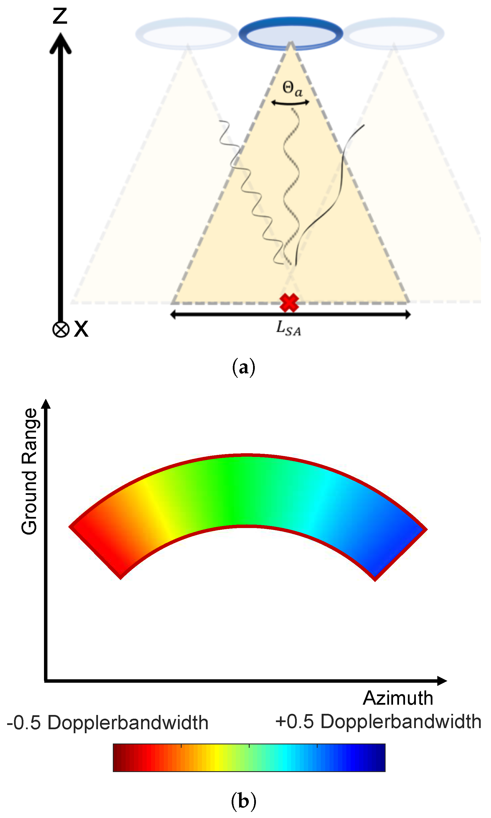
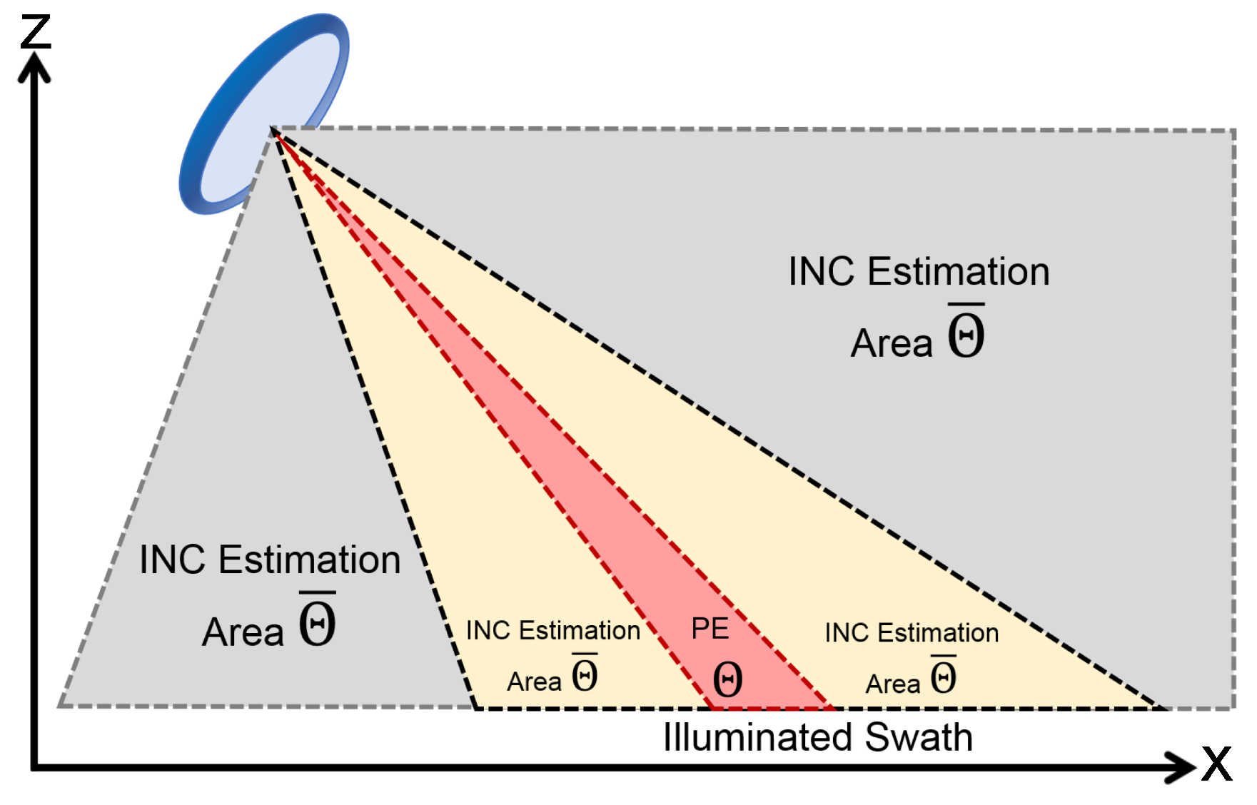
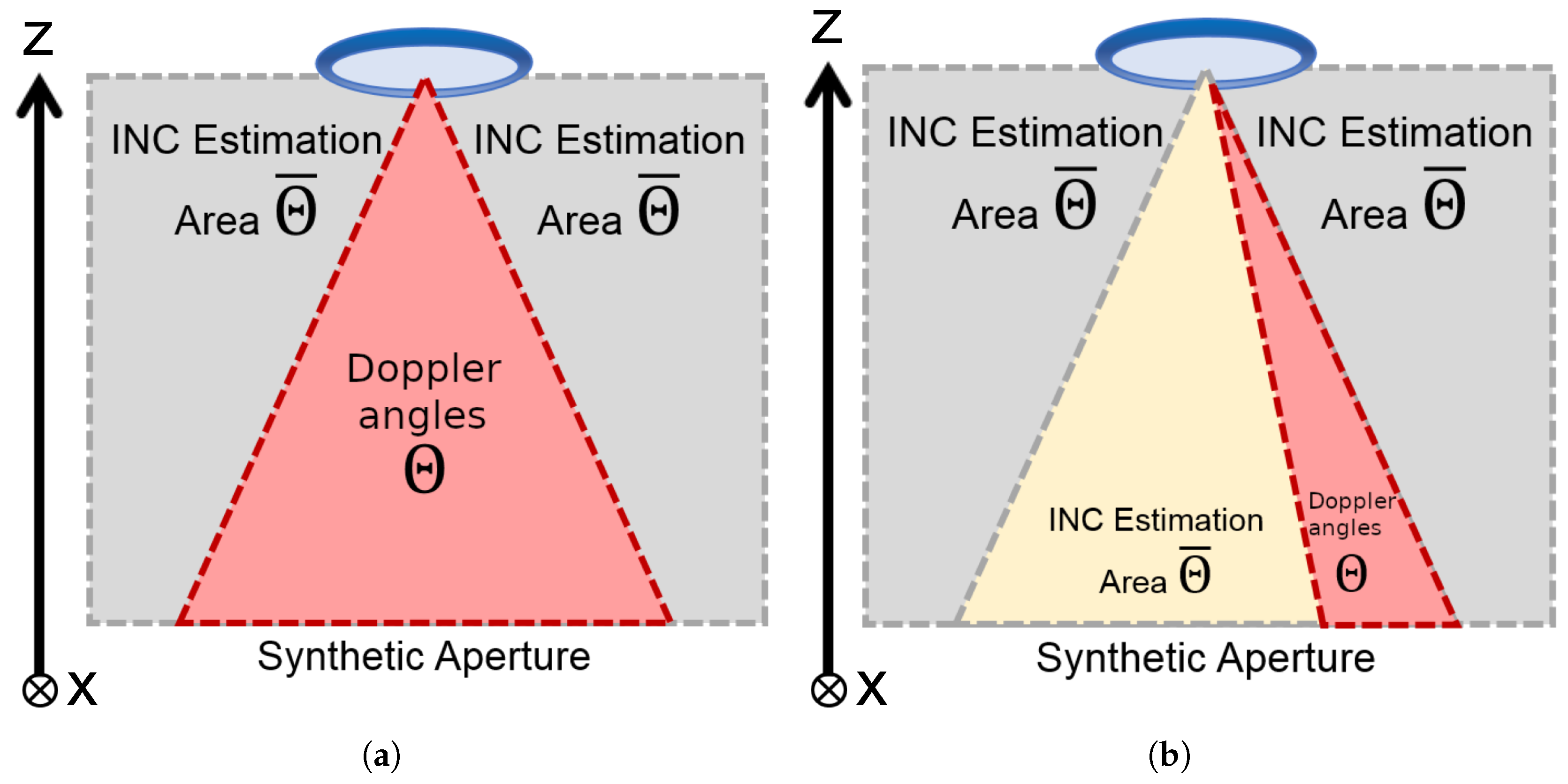
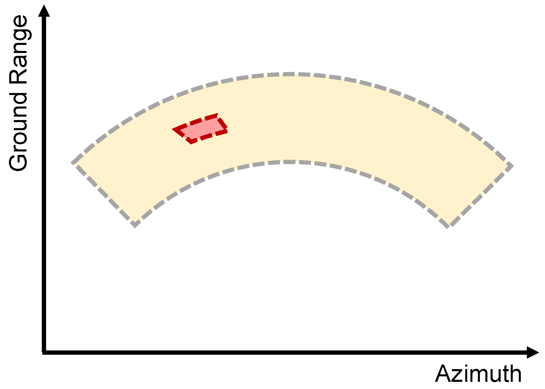
2.3. The Angular Extension of SAR Signals
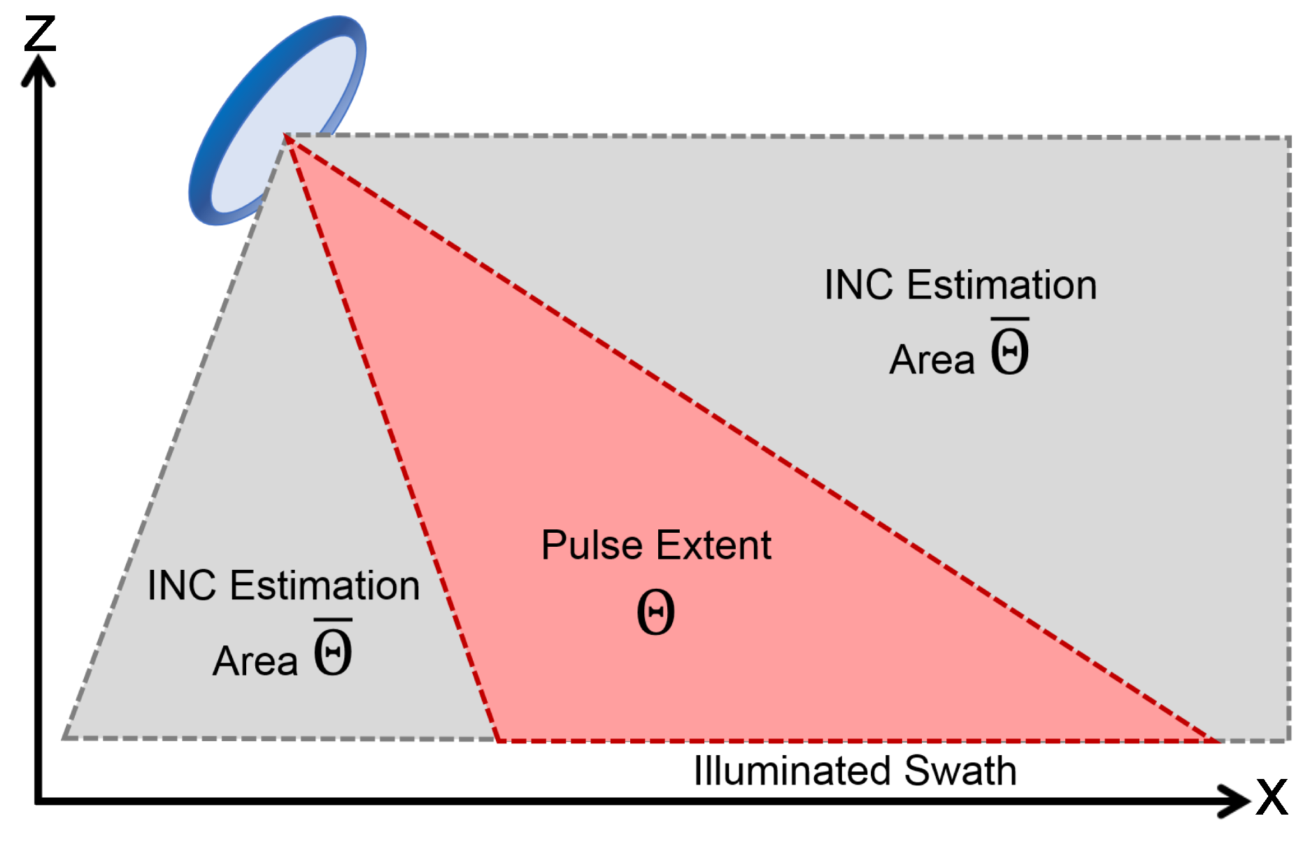
2.4. The Impact of Range Compression on the Angular Signal Extension
3. Proposed RFI Mitigation Algorithms Using DBF
3.1. DBF in Elevation
3.1.1. Pulse-Wise MVDR
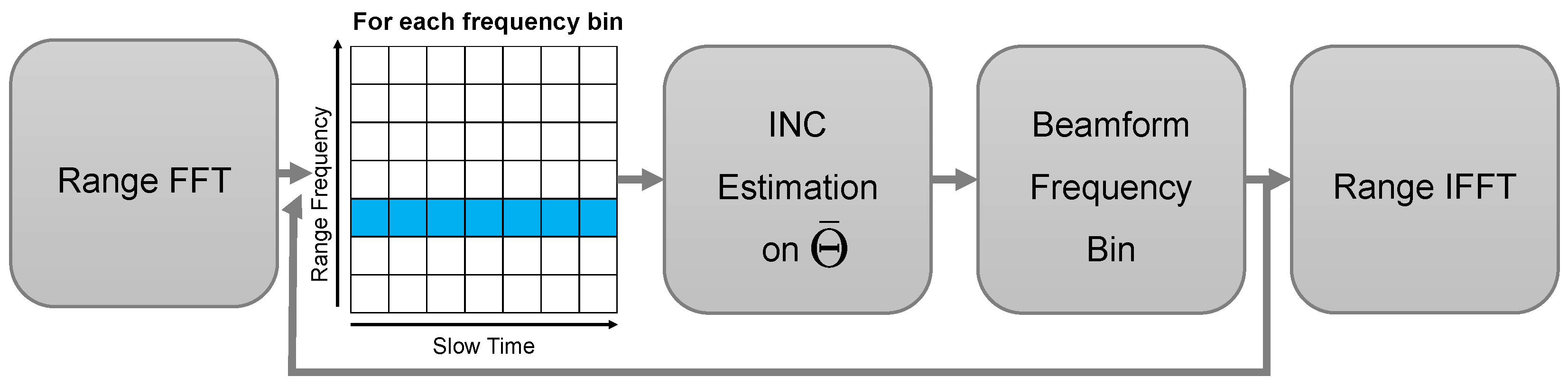
3.1.2. Segment-Wise Frequency MVDR
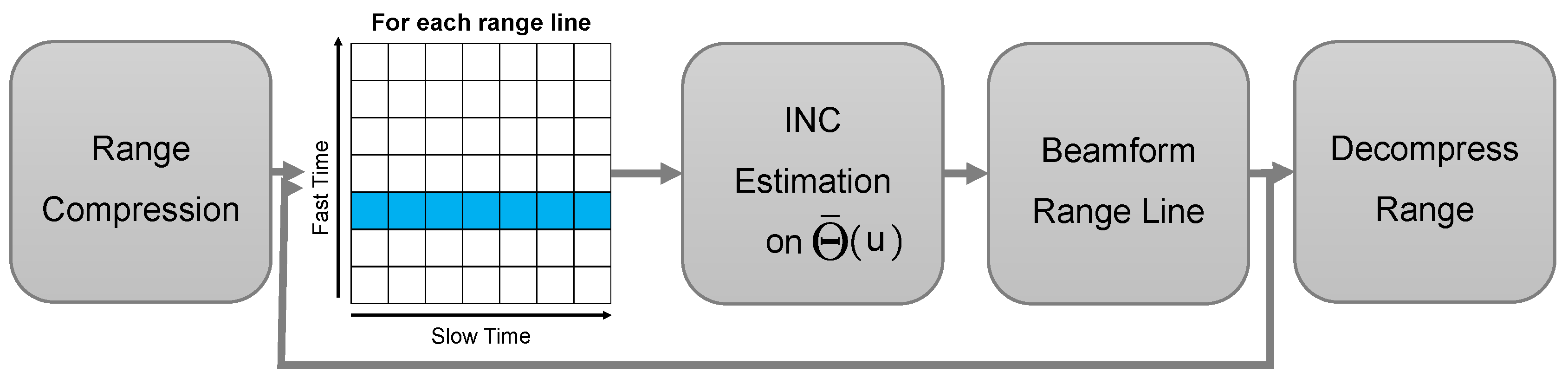
3.1.3. Range-Dependent Time MVDR
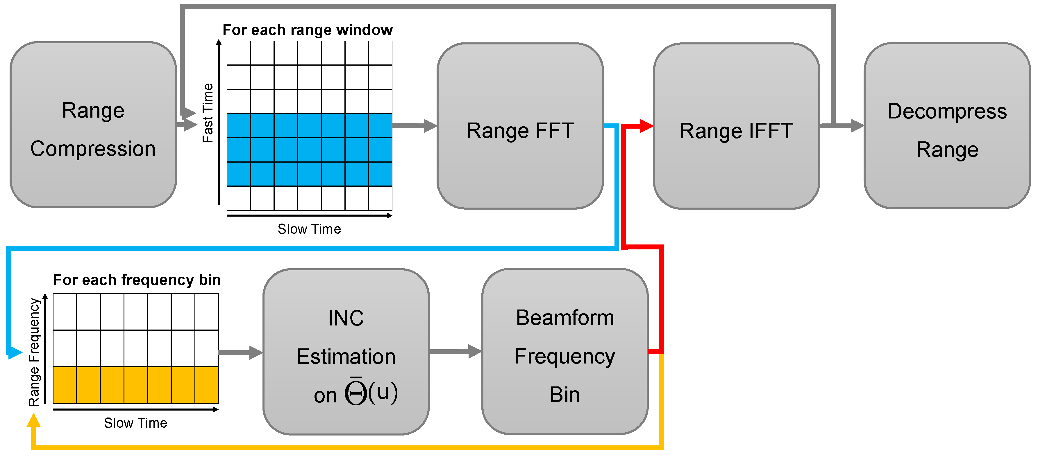
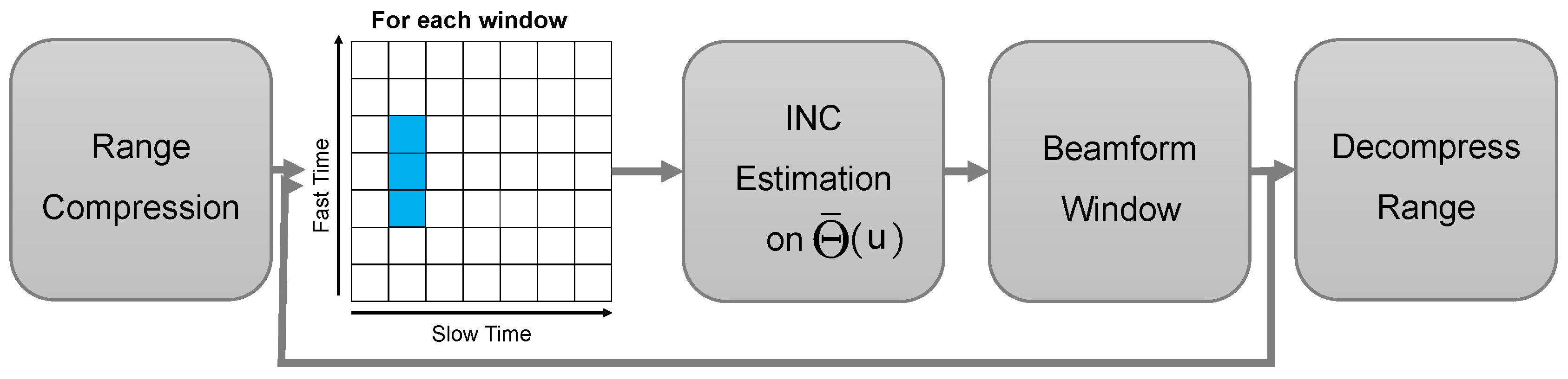
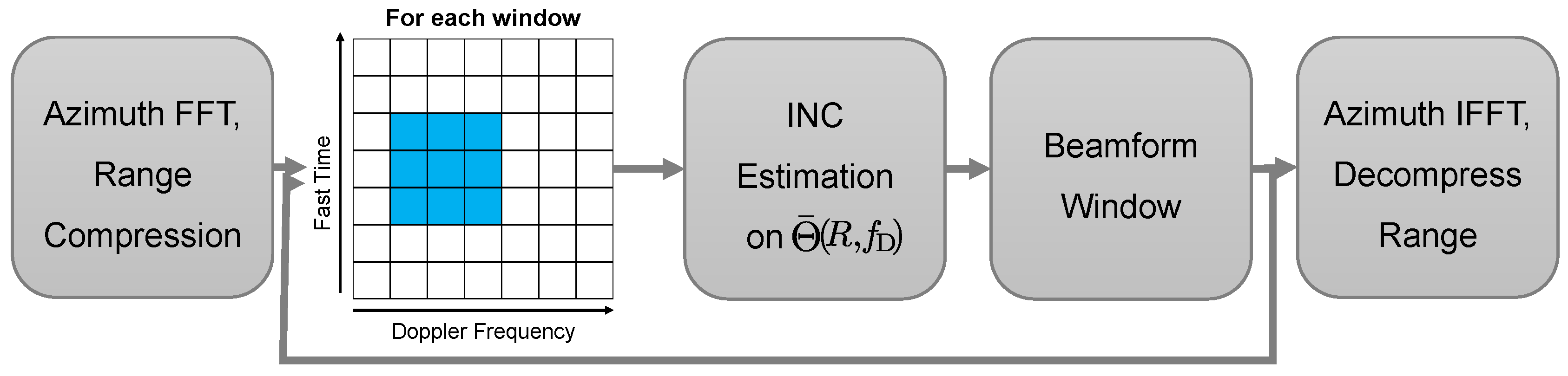
3.1.4. Range-Dependent Frequency MVDR
3.1.5. On the Utilization of Range-Frequency Sublooks
3.1.6. Pulsed-RFI MVDR
3.2. DBF in Azimuth
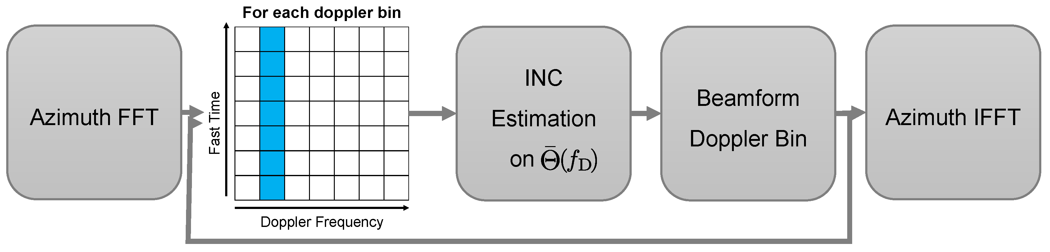
3.2.1. Doppler-Dependent MVDR
3.2.2. Doppler-Dependent Frequency MVDR
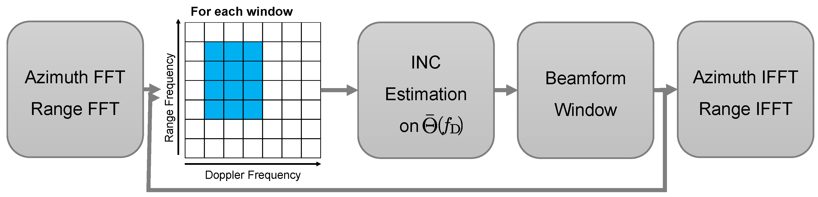
3.3. Two-Dimensional DBF
3.4. Summary
4. Simulations for DBF in Elevation
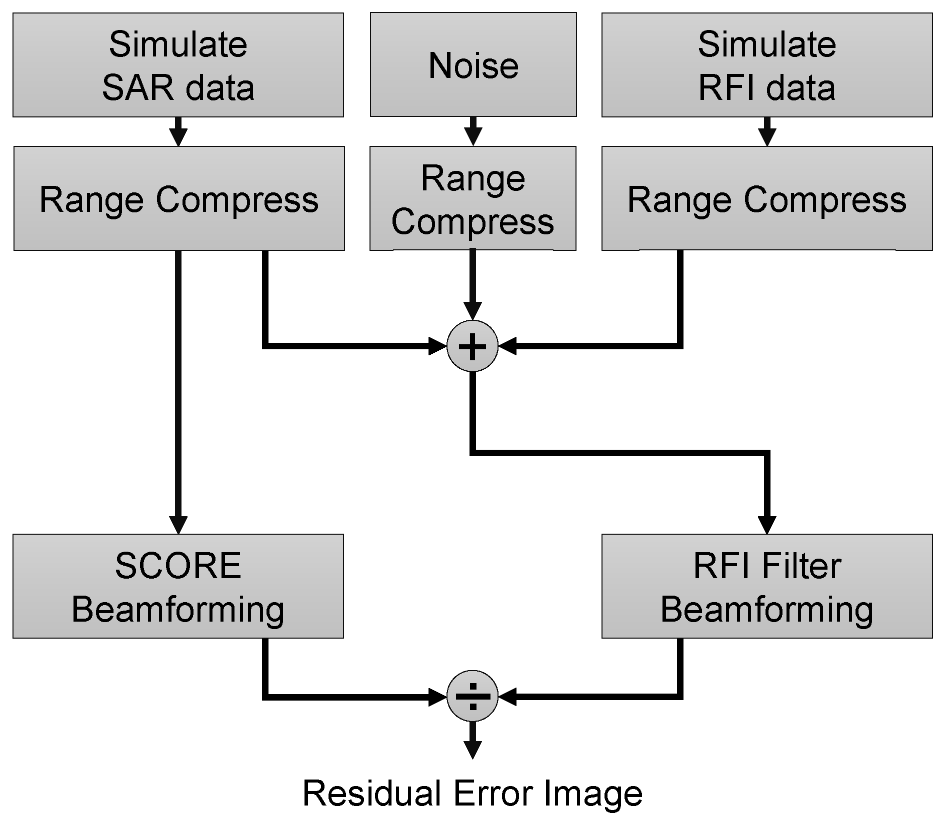
4.1. Simulation Steps and Parameters
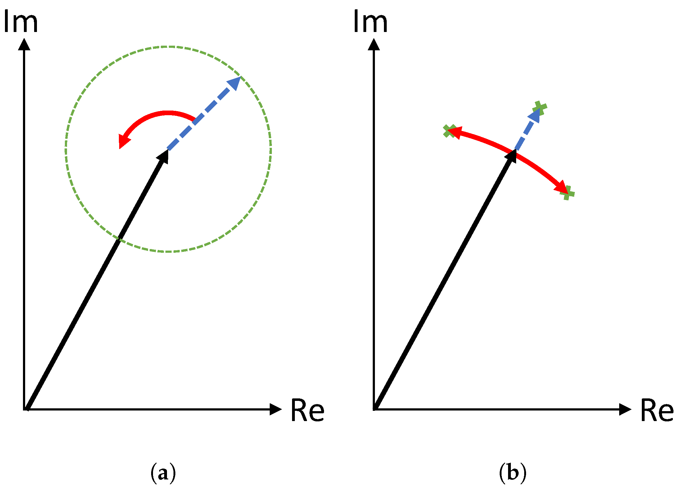
4.2. Error Model
4.3. Simulated Interference Scenarios
4.3.1. Scenario A
4.3.2. Scenario B
4.3.3. Scenario C
4.3.4. Scenario D
4.4. Simulation Results
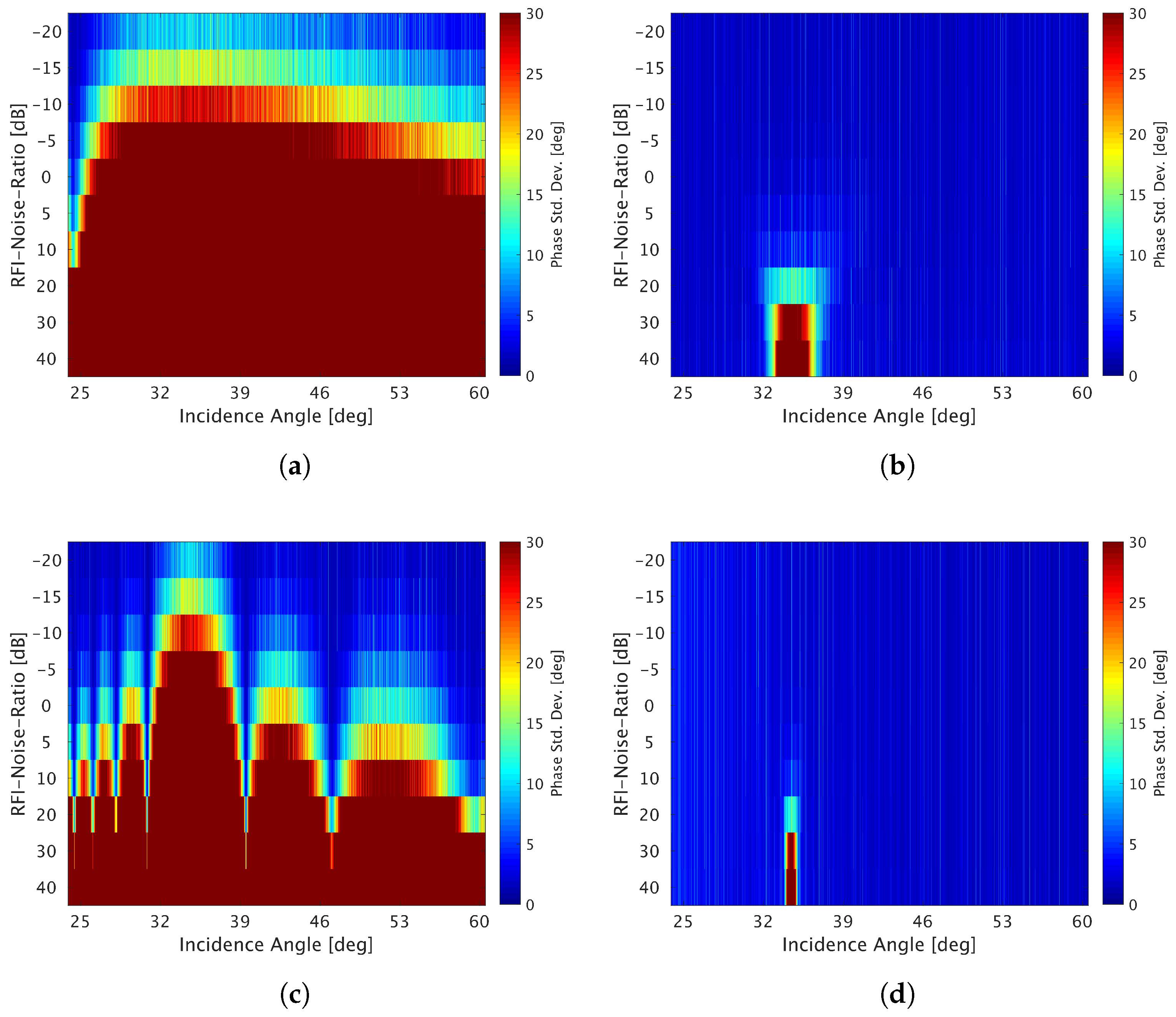
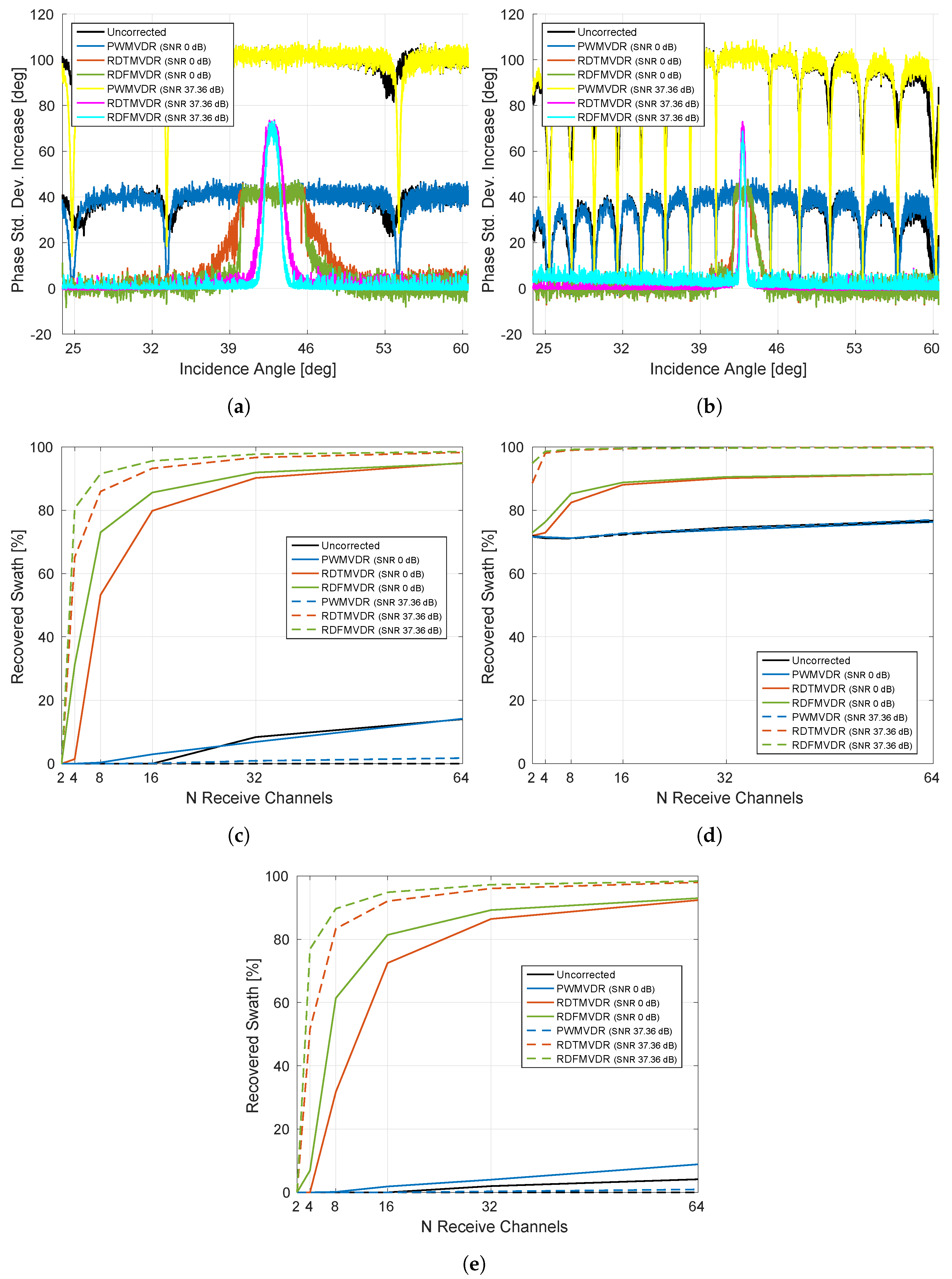
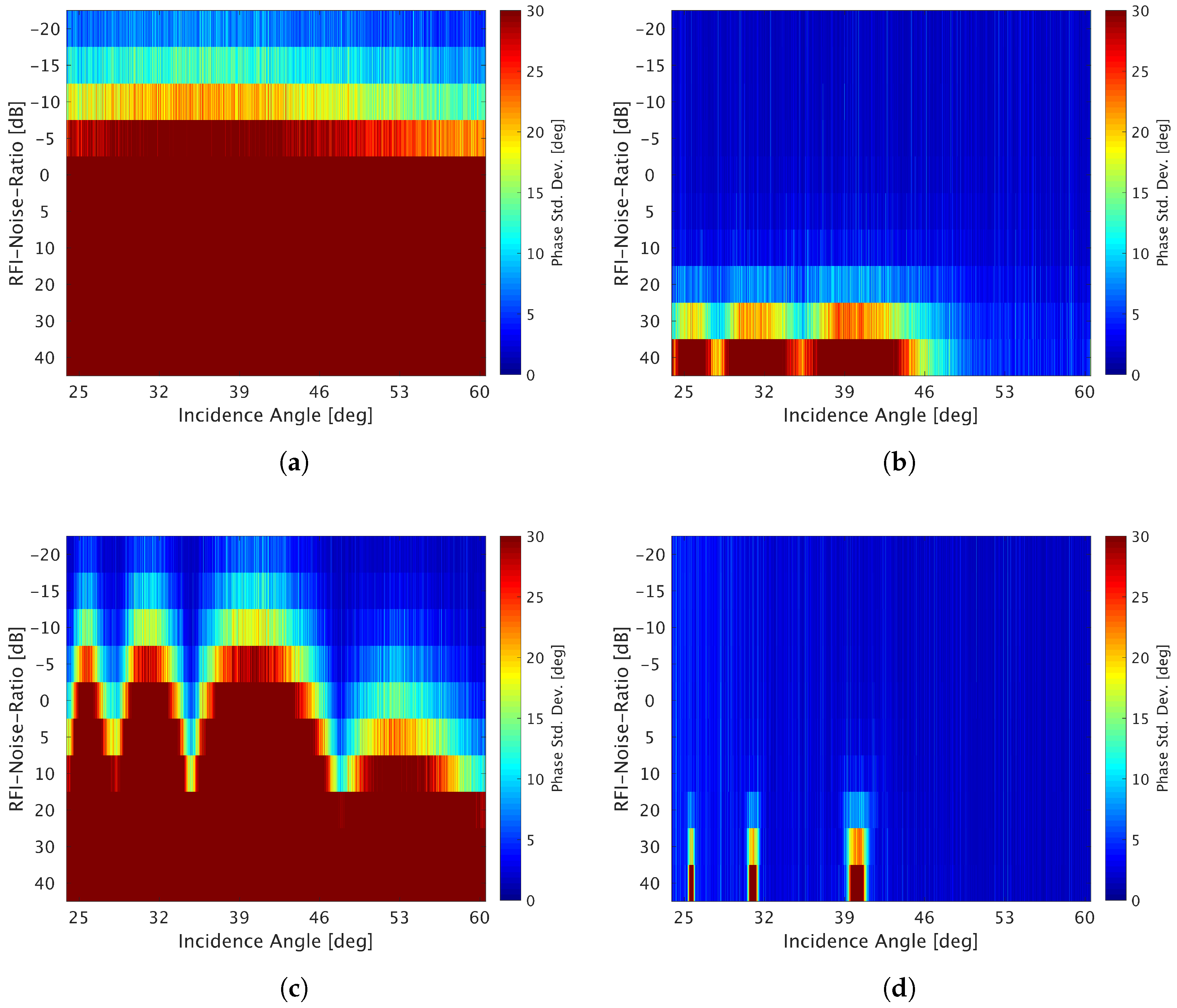
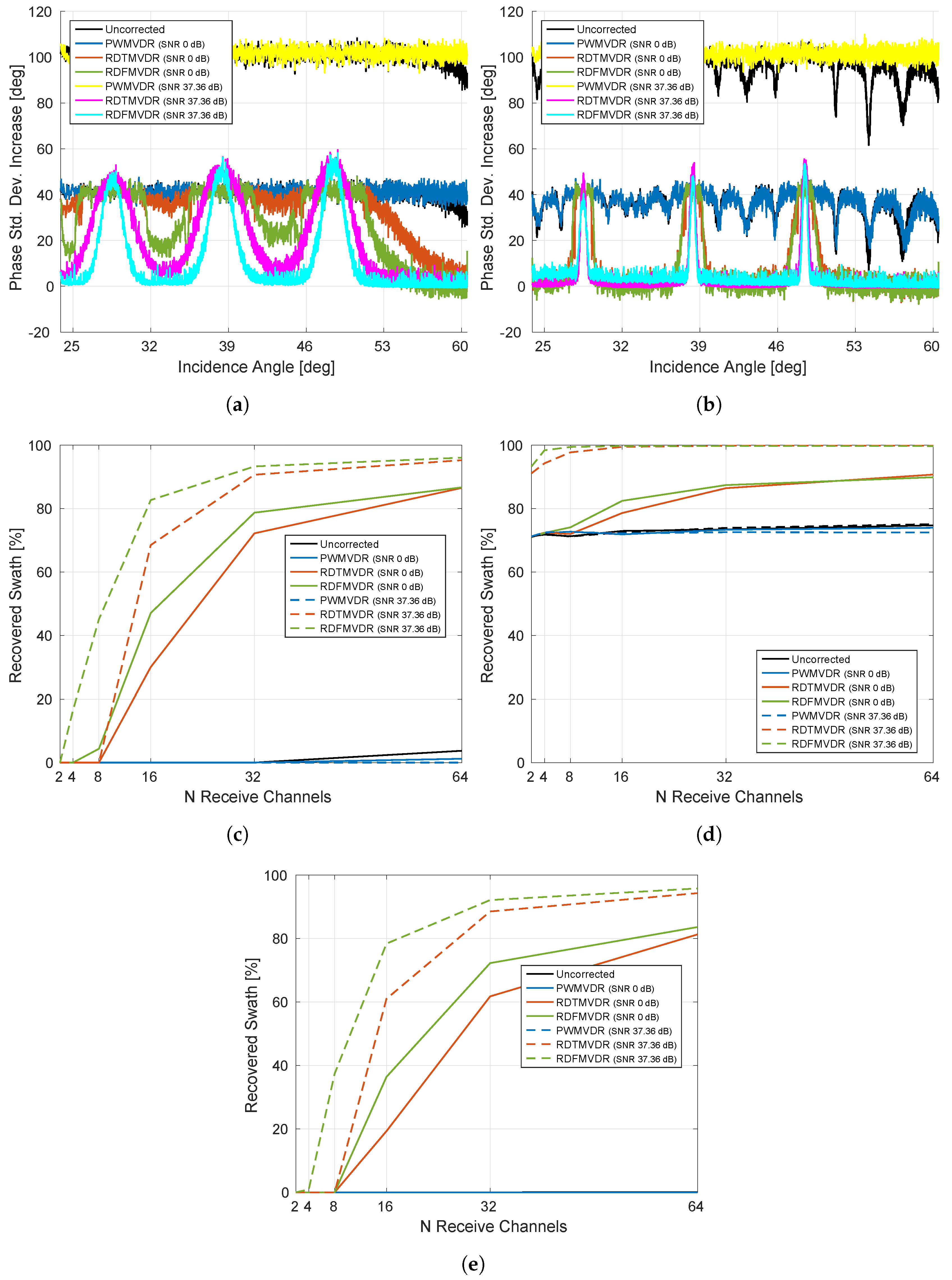
4.4.1. Scenario A
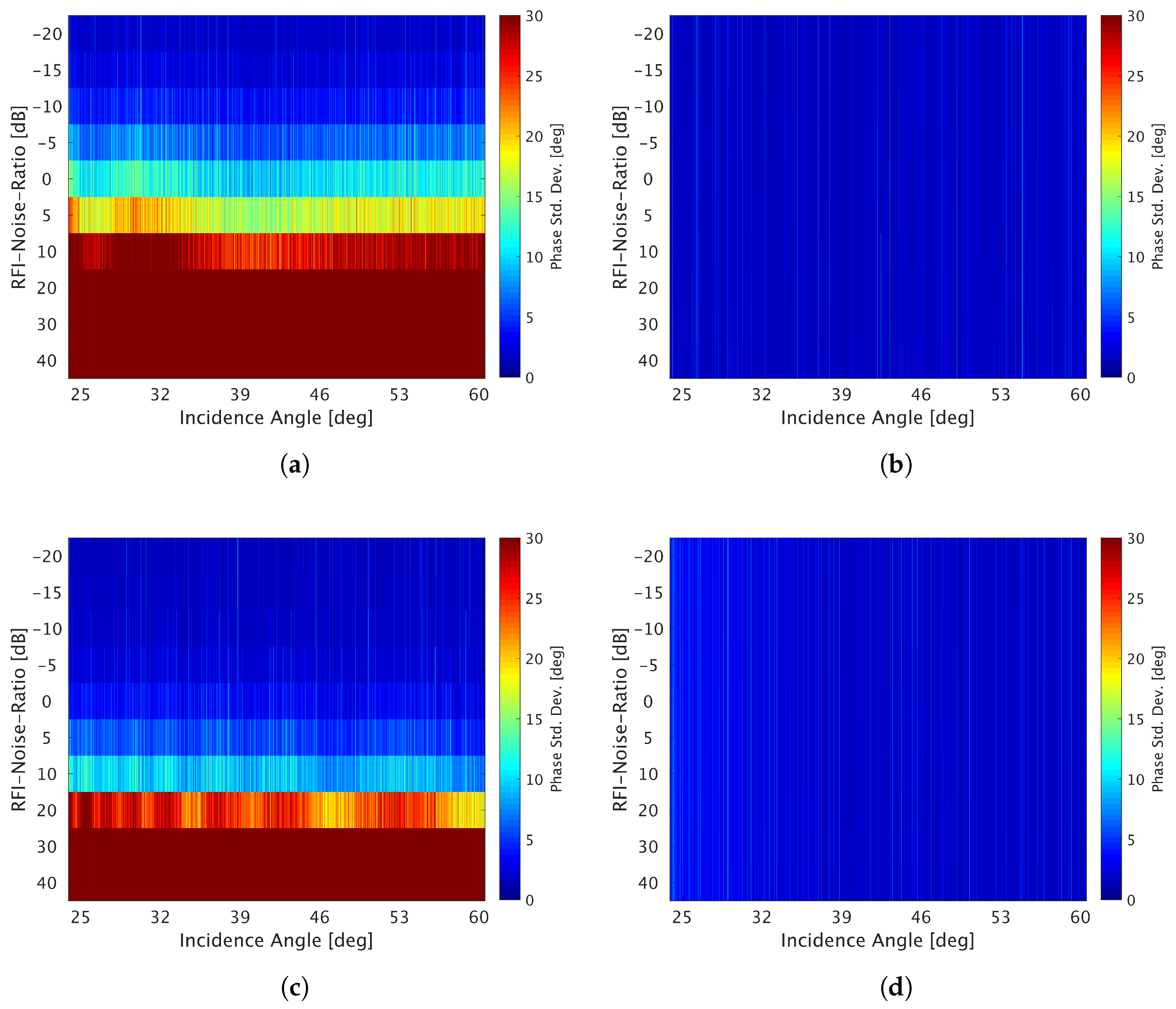
4.4.2. Scenario B
4.4.3. Scenario C
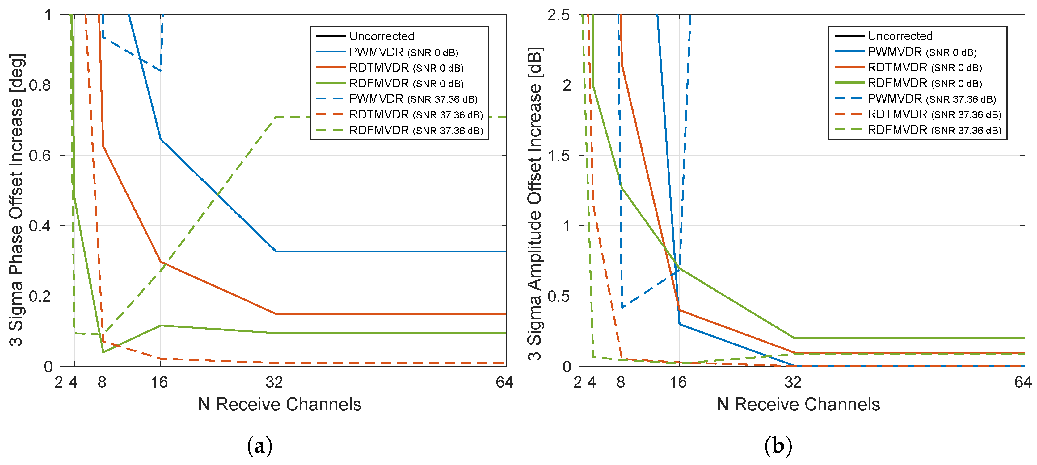
4.4.4. Scenario D
5. Experimental Results
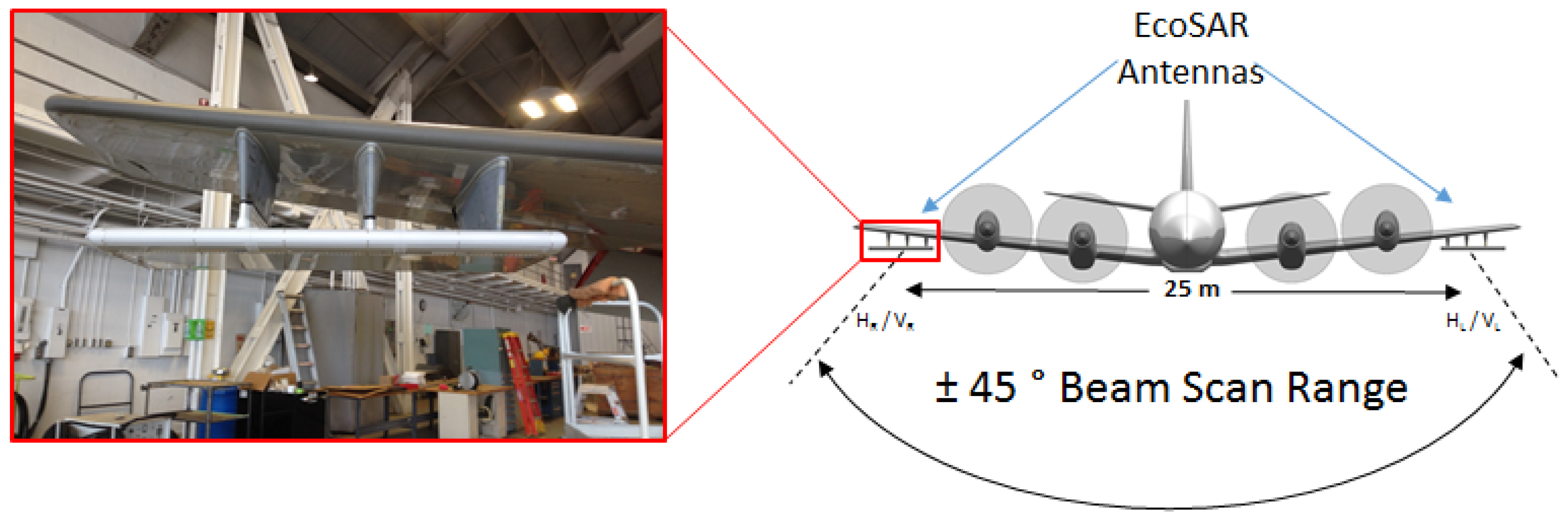
5.1. EcoSAR System Description
5.2. Dataset Description
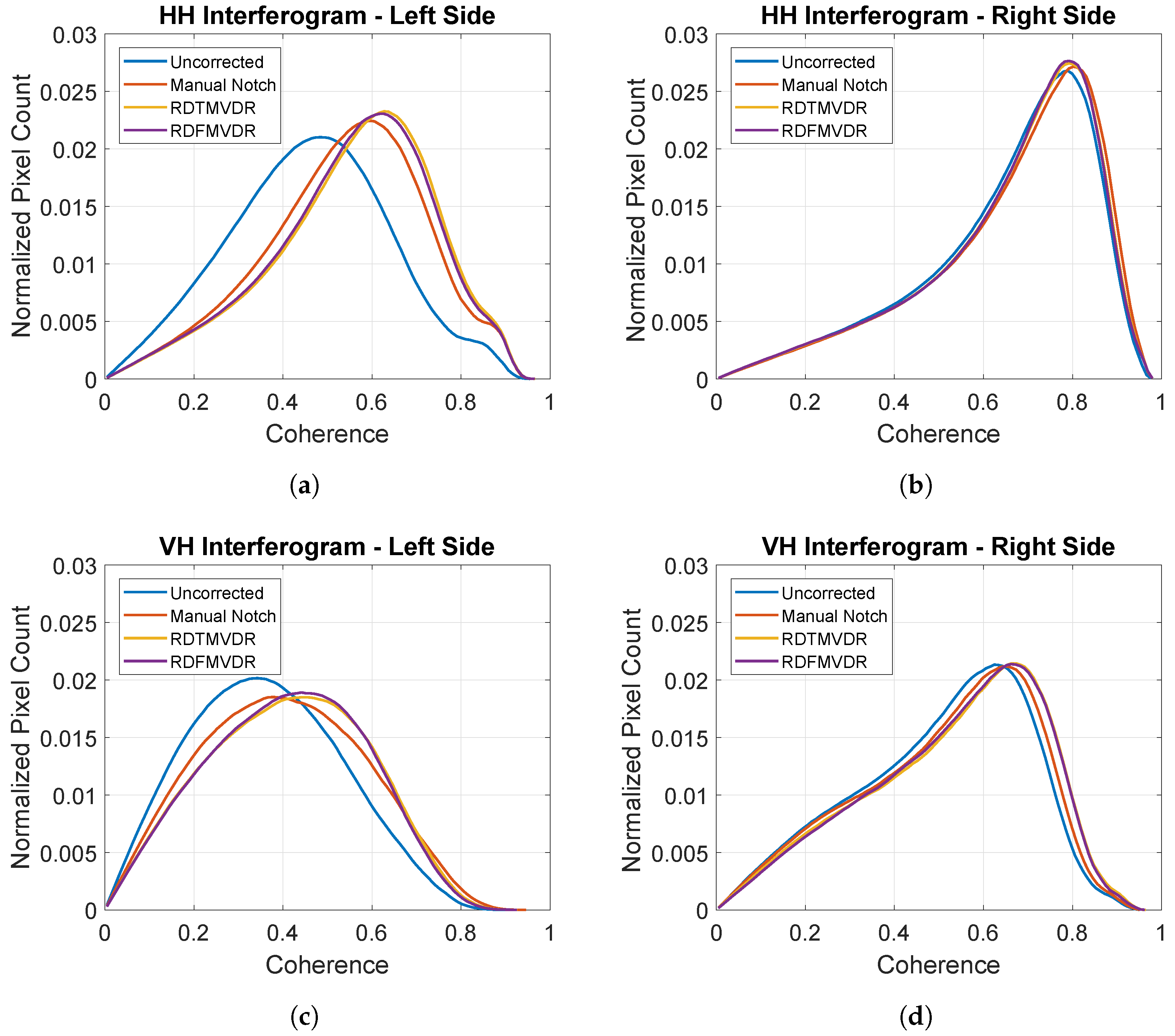
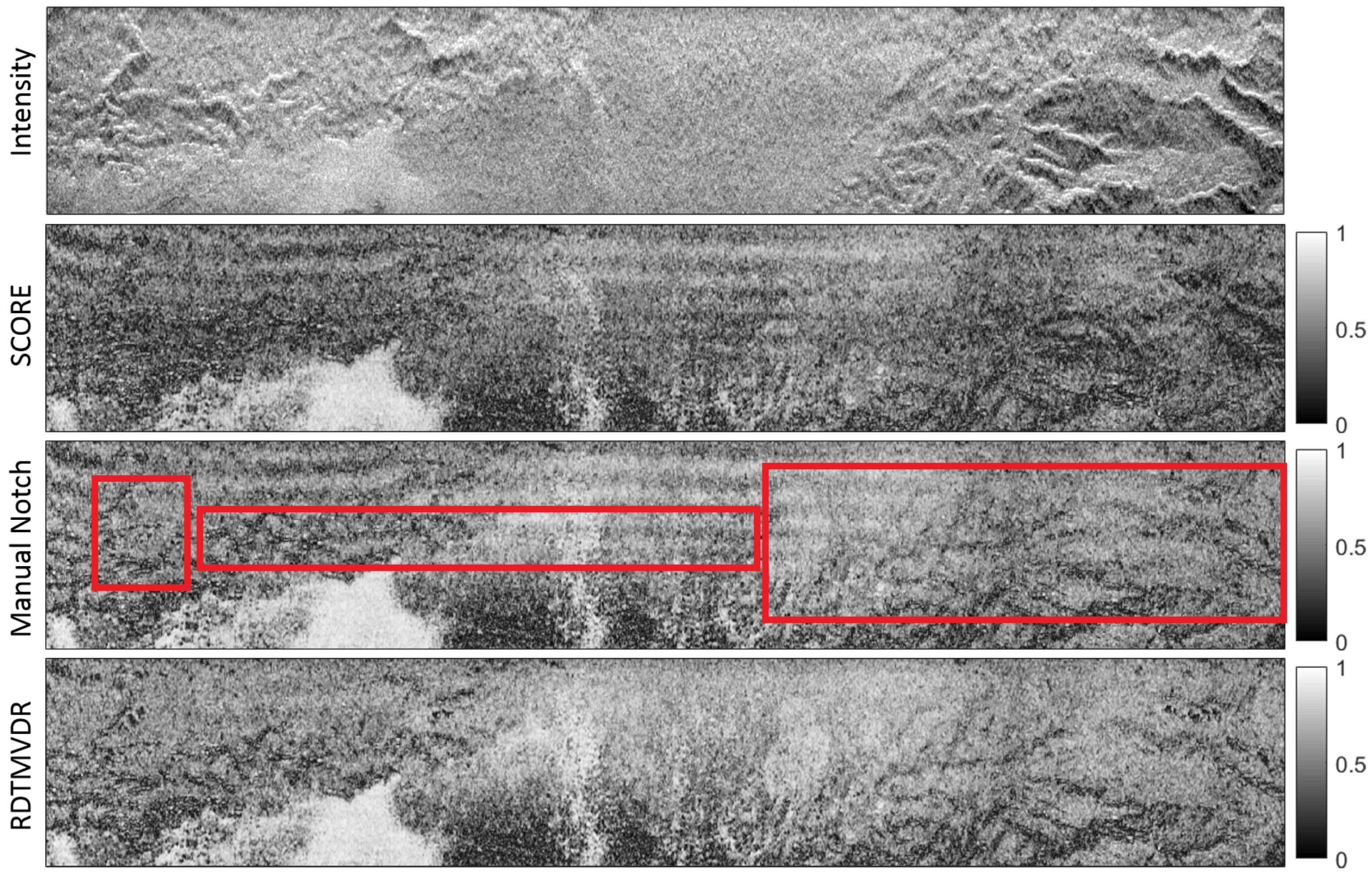
5.3. Results
6. Conclusions
Author Contributions
Funding
Conflicts of Interest
References
- Mazar, H. Radio Spectrum Management: Policies, Regulations and Techniques; John Wiley & Sons: Somerset, UK, 2016. [Google Scholar] [CrossRef]
- Radio Regulations; ITU: Geneva, Switzerland, 2016.
- ITU-R. Recommendation ITU-R RS.1260-1. Feasibility of Sharing Between Active Spaceborne Sensors and Other Services in the Range 420–470 MHz; International Telecommunication Union: Geneva, Switzerland, 2003. [Google Scholar]
- Shimada, M.; Isoguchi, O.; Tadono, T.; Isono, K. PALSAR Radiometric and Geometric Calibration. IEEE Trans. Geosci. Remote Sens. 2009, 47, 3915–3932. [Google Scholar] [CrossRef]
- Rosen, P.A.; Hensley, S.; Le, C. Observations and mitigation of RFI in ALOS PALSAR SAR data: Implications for the DESDynI mission. In Proceedings of the 2008 IEEE Radar Conference, Rome, Italy, 26–30 May 2008; pp. 1–6. [Google Scholar] [CrossRef]
- Meyer, F.J.; Nicoll, J.B.; Doulgeris, A.P. Correction and Characterization of Radio Frequency Interference Signatures in L-Band Synthetic Aperture Radar Data. IEEE Trans. Geosci. Remote Sens. 2013, 51, 4961–4972. [Google Scholar] [CrossRef] [Green Version]
- Lord, R.T.; Inggs, M.R. Approaches to RF interference suppression for VHF/UHF synthetic aperture radar. In Proceedings of the 1998 South African Symposium on Communications and Signal Processing, Rondebosch, South Africa, 8 September 1998; pp. 95–100. [Google Scholar] [CrossRef]
- Chang, J.L.; Li, X. The Effect of Notch Filter on RFI Suppression. Wirel. Sens. Netw. 2009, 1, 196–205. [Google Scholar] [CrossRef]
- Reigber, A.; Ferro-Famil, L. Interference suppression in synthesized SAR images. IEEE Geosci. Remote Sens. Lett. 2005, 2, 45–49. [Google Scholar] [CrossRef]
- Potsis, A.; Reigber, A.; Papathanassiou, K.P. A phase preserving method for RF interference suppression in P-band synthetic aperture radar interferometric data. In Proceedings of the IGARSS ’99 IEEE International Geoscience and Remote Sensing Symposium, Hamburg, Germany, 28 June–2 July 1999; Volume 5, pp. 2655–2657. [Google Scholar] [CrossRef]
- Braunstein, M.; James, M.; Ralston, D.A.S. Signal processing approaches to radio frequency interference (RFI) suppression. In Proceedings of the SPIE’s International Symposium on Optical Engineering and Photonics in Aerospace Sensing, Orlando, FL, USA, 4–8 April 1994; Volume 2230. [Google Scholar] [CrossRef]
- Lord, R.T.; Inggs, M.R. Efficient RFI suppression in SAR using LMS adaptive filter integrated with range/Doppler algorithm. Electron. Lett. 1999, 35, 629–630. [Google Scholar] [CrossRef]
- Le, C.T.C.; Hensley, S.; Chapin, E. Removal of RFI in wideband radars. In Proceedings of the IGARSS ’98 IEEE International Geoscience and Remote Sensing Symposium Proceedings, Seattle, WA, USA, 6–10 July 1998; Volume 4, pp. 2032–2034. [Google Scholar] [CrossRef]
- Applebaum, S. Adaptive arrays. IEEE Trans. Antennas Propag. 1976, 24, 585–598. [Google Scholar] [CrossRef]
- Farina, A. Single Sidelobe Canceller: Theory and Evaluation. IEEE Trans. Aerosp. Electron. Syst. 1977, AES-13, 690–699. [Google Scholar] [CrossRef]
- Farina, A. Evaluation of sidelobe-canceller performance. Commun. Radar Signal Process. IEE Proc. F 1982, 129, 52–58. [Google Scholar] [CrossRef]
- Sedehi, M.; Cristallini, D.; Marini, J.; Lombardo, P. Impact of an Electromagnetic Interference on Imaging Capability of a Synthetic Aperture Radar. In Proceedings of the 2007 IEEE Aerospace Conference, Big Sky, MT, USA, 3–10 March 2007; pp. 1–8. [Google Scholar] [CrossRef]
- Sedehi, M.; Colone, F.; Cristallini, D.; Lombardo, P. A reduced order jammer cancellation scheme based on double adaptivity. In Proceedings of the 2008 IEEE Radar Conference, Rome, Italy, 26–30 May 2008; pp. 1–6. [Google Scholar] [CrossRef]
- Lombardo, P.; Sedehi, M.; Colone, F.; Bucciarelli, M.; Cristallini, D. Dual Channel Adaptive Antenna Nulling with Auxiliary Selection for Spaceborne Radar. In Proceedings of the 2008 IEEE Aerospace Conference, Big Sky, MT, USA, 1–8 March 2008; pp. 1–8. [Google Scholar] [CrossRef]
- Sedehi, M.; Cristallini, D.; Bucciarelli, M.; Lombardo, P. Constrained adaptive beamforming for electromagnetic interference cancellation for a synthetic aperture radar. In Proceedings of the IET International Conference on Radar Systems, Edinburgh, UK, 15–18 October 2007; pp. 1–5. [Google Scholar] [CrossRef]
- Rincon, R.F.; Fatoyinbo, T.; Osmanoglu, B.; Lee, S.; Ranson, K.J.; Sun, G.; Bollian, T. ECOSAR: P-Band Digital Beamforming Polarimetric and Single Pass Interferometric SAR: Instrument Performance. In Proceedings of the EUSAR 2016: 11th European Conference on Synthetic Aperture Radar, Hamburg, Germany, 6–9 June 2016; pp. 1–5. [Google Scholar]
- Rincon, R.F.; Fatoyinbo, T.; Ranson, J.; Sun, G.; Perrine, M.; Bonds, Q.; Valett, S.; Seufert, S. Digital Beamforming Synthetic Aperture Radar (DBSAR) polarimetric operation during the Eco3D flight campaign. In Proceedings of the IEEE International Geoscience and Remote Sensing Symposium, Munich, Germany, 22–27 July 2012; pp. 1549–1552. [Google Scholar] [CrossRef]
- Younis, M.; Huber, S.; Herrero, C.T.; Krieger, G.; Moreira, A.; Uematsu, A.; Sudo, Y.; Nakamura, R.; Chishiki, Y.; Shimada, M. Tandem-L instrument design and SAR performance overview. In Proceedings of the 2014 IEEE Geoscience and Remote Sensing Symposium, Quebec City, QC, Canada, 13–18 July 2014; pp. 88–91. [Google Scholar] [CrossRef]
- Younis, M.; Fischer, C.; Wiesbeck, W. Digital beamforming in SAR systems. IEEE Trans. Geosci. Remote Sens. 2003, 41, 1735–1739. [Google Scholar] [CrossRef]
- Veen, B.D.V.; Buckley, K.M. Beamforming: A versatile approach to spatial filtering. IEEE ASSP Mag. 1988, 5, 4–24. [Google Scholar] [CrossRef]
- Suess, M.; Grafmueller, B.; Zahn, R. A novel high resolution, wide swath SAR system. In Proceedings of the IGARSS 2001, Scanning the Present and Resolving the Future, IEEE 2001 International Geoscience and Remote Sensing Symposium (Cat. No.01CH37217), Sydney, NSW, Australia, 9–13 July 2001; Volune 3, pp. 1013–1015. [Google Scholar] [CrossRef]
- Suess, M.; Wiesbeck, W. Side-looking Synthetic Aperture Radar System. European Patent EP 1241487 B1, 18 September 2006. [Google Scholar]
- Capon, J. High-resolution frequency-wavenumber spectrum analysis. Proc. IEEE 1969, 57, 1408–1418. [Google Scholar] [CrossRef]
- Trees, H. Optimum Array Processing (Detection, Estimation, and Modulation Theory, Part IV); Wiley-Interscience: New York, NY, USA, 2002. [Google Scholar]
- Lorenz, R.G.; Boyd, S.P. Robust minimum variance beamforming. IEEE Trans. Signal Process. 2005, 53, 1684–1696. [Google Scholar] [CrossRef] [Green Version]
- Cox, H. Resolving power and sensitivity to mismatch of optimum array processors. J. Acoust. Soc. Am. 1973, 54, 771–785. [Google Scholar] [CrossRef]
- Vural, A. Effects of perturbations on the performance of optimum/adaptive arrays. IEEE Trans. Aerosp. Electron. Syst. 1979, AES-15, 76–87. [Google Scholar] [CrossRef]
- Compton, R. The effect of random steering vector errors in the Applebaum adaptive array. IEEE Trans. Aerospa. Electron. Syst. 1982, AES-18, 392–400. [Google Scholar] [CrossRef]
- Wax, M.; Anu, Y. Performance analysis of the minimum variance beamformer in the presence of steering vector errors. IEEE Trans. Signal Process. 1996, 44, 938–947. [Google Scholar] [CrossRef]
- Bordoni, F.; Younis, M.; Varona, E.M.; Krieger, G. Adaptive scan-on-receive based on spatial spectral estimation for high-resolution, wide-swath Synthetic Aperture Radar. In Proceedings of the IEEE International Geoscience and Remote Sensing Symposium, Cape Town, South Africa, 12–17 July 2009; Volume 1, pp. I-64–I-67. [Google Scholar] [CrossRef]
- Frost, O.L. An algorithm for linearly constrained adaptive array processing. Proc. IEEE 1972, 60, 926–935. [Google Scholar] [CrossRef]
- Sedehi, M.; Bucciarelli, M.; Cristallini, D.; Scolamiero, S.; Lombardo, P. Interference covariance matrix estimation for a Multi-Channel Synthetic Aperture Radar. In Proceedings of the 7th European Conference on Synthetic Aperture Radar, Friedrichshafen, Germany, 2–5 June 2008; pp. 1–4. [Google Scholar]
- Villano, M.; Krieger, G.; Moreira, A. Staggered SAR: High-resolution wide-swath imaging by continuous PRI variation. IEEE Trans. Geosci. Remote Sens. 2014, 52, 4462–4479. [Google Scholar] [CrossRef]
- Villano, M.; Krieger, G.; Moreira, A. A novel processing strategy for staggered SAR. IEEE Geosci. Remote Sens. Lett. 2014, 11, 1891–1895. [Google Scholar] [CrossRef]
- Villano, M.; Krieger, G.; Jäger, M.; Moreira, A. Staggered SAR: Performance Analysis and Experiments with Real Data. IEEE Trans. Geosci. Remote Sens. 2017, 55, 6617–6638. [Google Scholar] [CrossRef]
- De Almeida, F.Q.; Younis, M.; Krieger, G.; Moreira, A. Multichannel staggered SAR azimuth processing. IEEE Trans. Geosci. Remote Sens. 2018, 56, 2772–2788. [Google Scholar] [CrossRef]
- Gu, Y.; Leshem, A. Robust adaptive beamforming based on interference covariance matrix reconstruction and steering vector estimation. IEEE Trans. Signal Process. 2012, 60, 3881–3885. [Google Scholar]
- Younis, M.; Rommel, T.; Bordoni, F.; Krieger, G.; Moreira, A. On the pulse extension loss in digital beamforming SAR. IEEE Geosci. Remote Sens. Lett. 2015, 12, 1436–1440. [Google Scholar] [CrossRef]
- Moreira, A. Radar Mit Synthetischer Apertur; Oldenbourg Verlag: München, Germany, 1999. [Google Scholar]
- Schmidt, R. Multiple emitter location and signal parameter estimation. IEEE Trans. Antennas Propag. 1986, 34, 276–280. [Google Scholar] [CrossRef] [Green Version]
- Wu, H.T.; Yang, J.F.; Chen, F.K. Source number estimators using transformed Gerschgorin radii. IEEE Trans. Signal Process. 1995, 43, 1325–1333. [Google Scholar] [CrossRef]
- Qiu, Z.; He, Z.; Cui, M. A method for signal source number estimation based on MUSIC algorithm. In Proceedings of the IEEE International Conference on Communication Problem-Solving (ICCP), Guilin, China, 16–18 October 2015; pp. 344–346. [Google Scholar] [CrossRef]
- Rapuano, S.; Harris, F.J. An introduction to FFT and time domain windows. IEEE Instrum. Meas. Mag. 2007, 10, 32–44. [Google Scholar] [CrossRef]
- Yegulalp, A.F. Fast backprojection algorithm for synthetic aperture radar. In Proceedings of the 1999 IEEE Radar Conference. Radar into the Next Millennium (Cat. No.99CH36249), Waltham, MA, USA, 22–22 April 1999; pp. 60–65. [Google Scholar] [CrossRef]
- Duersch, M.I. Backprojection for Synthetic Aperture Radar; Brigham Young University: Provo, UT, USA, 2013. [Google Scholar]
- Rincon, R.F.; Fatoyinbo, T.; Ranson, K.J.; Osmanoglu, B.; Sun, G.; Deshpande, M.; Perrine, M.; Toit, C.D.; Bonds, Q.; Beck, J.; et al. The ecosystems SAR (EcoSAR) an airborne P-band polarimetric InSAR for the measurement of vegetation structure, biomass and permafrost. In Proceedings of the IEEE Radar Conference, Cincinnati, OH, USA, 19–23 May 2014; pp. 1443–1445. [Google Scholar] [CrossRef]
- Rincon, R.F.; Fatoyinbo, T.; Osmanoglu, B.; Lee, S.; Ranson, K.J.; Sun, G.; Perrine, M.; Toit, C.D. ECOSAR: P-band digital beamforming polarimetric and single pass interferometric SAR. In Proceedings of the IEEE Radar Conference (RadarCon), Arlington, VA, USA, 10–15 May 2015; pp. 0699–0703. [Google Scholar] [CrossRef]
- Osmanoglu, B.; Rincon, R.; Lee, S.; Bollian, T.; Fatoyinbo, T. Forest structure retrieval from EcoSAR P-band single-pass interferometry. In Proceedings of the IEEE International Geoscience and Remote Sensing Symposium (IGARSS), Fort Worth, TX, USA, 23–28 July 2017; pp. 4296–4305. [Google Scholar] [CrossRef]
- Carreiras, J.M.; Quegan, S.; Toan, T.L.; Minh, D.H.T.; Saatchi, S.S.; Carvalhais, N.; Reichstein, M.; Scipal, K. Coverage of high biomass forests by the ESA BIOMASS mission under defense restrictions. Remote Sens. Environ. 2017, 196, 154–162. [Google Scholar] [CrossRef]
- Toan, T.L.; Quegan, S.; Davidson, M.; Balzter, H.; Paillou, P.; Papathanassiou, K.; Plummer, S.; Rocca, F.; Saatchi, S.; Shugart, H.; et al. The BIOMASS mission: Mapping global forest biomass to better understand the terrestrial carbon cycle. Remote Sens. Environ. 2011, 115, 2850–2860. [Google Scholar] [CrossRef] [Green Version]
- Dubois-Fernandez, P.C.; Toan, T.L.; Daniel, S.; Oriot, H.; Chave, J.; Blanc, L.; Villard, L.; Davidson, M.W.J.; Petit, M. The TropiSAR Airborne Campaign in French Guiana: Objectives, Description, and Observed Temporal Behavior of the Backscatter Signal. IEEE Trans. Geosci. Remote Sens. 2012, 50, 3228–3241. [Google Scholar] [CrossRef]
- Bollian, T.; Osmanoglu, B.; Rincon, R.F.; Lee, S.; Fatoyinbo, T.E. Detection and Geolocation ofP-Band Radio Frequency Interference Using EcoSAR. IEEE J. Sel. Top. Appl. Earth Obs. Remote Sens. 2018, 11, 3608–3616. [Google Scholar] [CrossRef]
- Krieger, G.; Gebert, N.; Moreira, A. Multidimensional Waveform Encoding: A New Digital Beamforming Technique for Synthetic Aperture Radar Remote Sensing. IEEE Trans. Geosci. Remote Sens. 2008, 46, 31–46. [Google Scholar] [CrossRef]
- Krieger, G. MIMO-SAR: Opportunities and Pitfalls. IEEE Trans. Geosci. Remote Sens. 2014, 52, 2628–2645. [Google Scholar] [CrossRef]
- Krieger, G.; Huber, S.; Villano, M.; Younis, M.; Rommel, T.; Dekker, P.L.; de Almeida, F.Q.; Moreira, A. CEBRAS: Cross elevation beam range ambiguity suppression for high-resolution wide-swath and MIMO-SAR imaging. In Proceedings of the IEEE International Geoscience and Remote Sensing Symposium (IGARSS), Milan, Italy, 26–31 July 2015; pp. 196–199. [Google Scholar] [CrossRef]


| Parameter | Value |
|---|---|
| Elevation Channels | 2 to 64 |
| Channel Spacing | 0.5 |
| Sample Frequency | 290 MHz |
| Center Frequency | 435 MHz |
| Pulse Bandwidth | 120 MHz |
| Pulse Duration | 20 s |
| Near Range Angle | 21° |
| Far Range Angle | 60° |
| Platform Altitude | 3.2 km |
| Number of Pulses | 500 |
| Backscatter Amplitude | Normal distribution with zero mean |
| Backscatter Phase | Uniform distribution from 0° to 360° |
| SNR | 0 dB, 37.63 dB |
| RFI Type | Continuous Wave |
| Algorithm | DBF Type | Placing of up to N-1 Nulls Per | RFI Type | Advantage | Disadvantage |
|---|---|---|---|---|---|
| Pulse-Wise | Elevation | per pulse | Both | Fast, for scenes without expected in-swath interference | Blind in-swath |
| Segment-Wise Frequency | Elevation | per frequency bin | Continuous | Fast, for scenes without expected in-swath interference | Blind in-swath |
| Range-Dependent Time | Elevation | per range line | Continuous | Recovers part of swath despite in-swath interference | Processing time |
| Range-Dependent Frequency | Elevation | per range window and frequency bin | Continuous | Recovers part of swath despite in-swath interference. Beneficial for smaller antenna arrays. | Increased processing time |
| Pulsed-RFI | Elevation | per range window | Pulsed | Suitable for pulsed RFI Scenarios. Recovers in-swath interference | Not detecting weak CW interference |
| Doppler Dependent | Azimuth | per Doppler frequency bin | Continuous | Fast, for scenes without expected in-swath interference | Blind in-swath |
| Doppler Dependent Frequency | Azimuth | per range-Doppler window | Both | Suitable for CW and pulsed in-swath interference | Processing time |
| 2D | Both | per range-Doppler window | Both | Capable of placing most notches and can recover largest swath percentage | Increased processing time |
| Capability | Dataset | |
|---|---|---|
| Center Frequency | 435 MHz | 479 MHz |
| Bandwidth | up to 120 MHz (H) up to 200 MHz (V) | 20 MHz |
| Pulse Length | 1 s to 50 s | 2.5 s (H) 1.5 s (V) |
| PRF | 100 Hz to 10 kHz | 500 Hz |
| Range Resolution | 0.75 m | 7.5 m |
| Azimuth Resolution | 0.5 m | 0.675 m |
| Array Power | 40 Watts | 40 Watts |
| Flight Altitude | 3.7 km | |
| Platform Velocity | 136 m/s | |
| Physical Baseline | 25 m | |
| Antenna elements | 8 per antenna | |
| Antenna element spacing | 0.29 cm (0.46) |
© 2019 by the authors. Licensee MDPI, Basel, Switzerland. This article is an open access article distributed under the terms and conditions of the Creative Commons Attribution (CC BY) license (http://creativecommons.org/licenses/by/4.0/).
Share and Cite
Bollian, T.; Osmanoglu, B.; Rincon, R.; Lee, S.-K.; Fatoyinbo, T. Adaptive Antenna Pattern Notching of Interference in Synthetic Aperture Radar Data Using Digital Beamforming. Remote Sens. 2019, 11, 1346. https://0-doi-org.brum.beds.ac.uk/10.3390/rs11111346
Bollian T, Osmanoglu B, Rincon R, Lee S-K, Fatoyinbo T. Adaptive Antenna Pattern Notching of Interference in Synthetic Aperture Radar Data Using Digital Beamforming. Remote Sensing. 2019; 11(11):1346. https://0-doi-org.brum.beds.ac.uk/10.3390/rs11111346
Chicago/Turabian StyleBollian, Tobias, Batuhan Osmanoglu, Rafael Rincon, Seung-Kuk Lee, and Temilola Fatoyinbo. 2019. "Adaptive Antenna Pattern Notching of Interference in Synthetic Aperture Radar Data Using Digital Beamforming" Remote Sensing 11, no. 11: 1346. https://0-doi-org.brum.beds.ac.uk/10.3390/rs11111346