New Workflow of Plastic-Mulched Farmland Mapping using Multi-Temporal Sentinel-2 data

Abstract

Using plastic film mulch on cropland improves crop yield in water-deficient areas, but the use of plastic film on cropland leads to soil pollution. The accurate mapping of plastic-mulched land (PML) is valuable for monitoring the environmental problems caused by the use of plastic film. The drawback of PML mapping is that the detectable period of PML changes among the fields, which causes uncertainty when supervised classification methods are used to identify PML. In this study, a new workflow which merging PML of multiple temporal phases (MTPML) is proposed. For each temporal phase, the “possible PML” is firstly generated, these “temporal possible PML” layers are then combined to generate the “possible PML” layer. Finally, the maximum normalized difference vegetation index (NDVI) of the growing season is used to remove the non-cropland pixels from the “possible PML layer,” and then generate PML images. When generating “temporal possible PML layers,” three new PML indices (PMLI with near-infrared bands known as PMLI_NIR, PMLI with shortwave infrared bands known as PMLI_SWIR, and Normalized Difference PMLI known as PMLI_ND) are proposed to separate PML from bare land at plastic film cover stage; and the “temporal possible PML layer” are identified by the threshold based method. To estimate the performance of the three PML indices, two other approaches, PMLI threshold and Random Forest (RF) are used to generate “temporal possible PML layer.” Finally, PML images generated from the five MTPML approaches are compared with the image time series supervised classification (SUPML) result. Two study regions, Hengshui (HS) and Guyuan (GY), are used in this study. PML identification models are generated using training samples in HS and the models are used for PML mapping in both study regions. The results showed that MTPML workflow outperformed SUPML with 3%–5% higher classification accuracy. The three proposed PML indices had higher separability and importance score for bare land and PML discrimination. Among the five approaches used to generate the “temporal possible PML layer,” PMLI_SWIR is the recommended approach because the PMLI_SWIR threshold approach is easy to implement and the accuracy is only slightly lower than the RF approach. It is notable that no training sample was used in GY and the accuracy of the MTPML approach was higher than 85%, which indicated that the rules proposed in this study are suitable for other study regions.

1. Introduction

Plastic mulch film has been widely used over soil surface to suppress weeds, conserve water, and regulate temperature during crop growth [1,2,3] and to improve the crop yield in arid/semi-arid regions [4,5,6,7]. However, the use of plastic mulch film also leads to environmental problems. For example, only 10% of the mulch film used in the fields are degradable and the plastic-film left in the fields lead to plastic pollution of the soil system [8,9,10], and the small plastic particles accumulated in soils could threaten soil quality, particularly in the regions with high plastic mulching application intensity [11]. Therefore, accurate data of the spatial distribution of plastic-mulched land (PML) at the local and regional scale is an important data source for both agricultural and environmental analyses.

Satellite observations can be used for land cover mapping even from regional to global scales [12,13]. However, most studies about plastic over the land surface are focused on plastic greenhouse (PG) mapping [14,15,16,17]. The identification of PML is more challenging than PG because, unlike greenhouses, which are not covered by the canopy during the growing season, PML is not detectable when the plants grow above the soil. Additionally, only a few studies have concentrated on mapping PML using satellite data. Hasituya and Chen [18] used multi-temporal Landsat-8 images and machine learning algorithms (Support Vector Machine and Random Forest) to identify PML, and found that the best temporal period for PML detection is between the time of planting and green-up [19,20]. To simplify the procedure of PML identification, a PML index (PMLI) has been proposed [15], PMLI have shown good potential to identify PML with a threshold using both Landsat and MODIS images. Comparing with the machine learning methods, the PMLI threshold method is easier to implement and more suitable for PML identification at large scale [15,21]. In addition, the performance of synthetic-aperture radar (SAR) images for PML identification have been evaluated. When only using the SAR features to identify PML, the classification accuracies are low, and when adding SAR feature into optical data, the PML identification accuracies just improve by 1%~3% [2,22], so that the optical features still have high contribution to PML identification.

However, existing PML identification techniques still have several disadvantages. First, PML is used for multiple crops and the sowing stage of these crops varies, so that the plastic-films are spread on fields at different time phases. Existing studies have tried to use image time-series to identify the PML, but the complex pattern of PML leads to misclassification when using time series data and supervised classification methods like Random Forest. Second, existing studies have used Landsat-8 and MODIS images for PML identification. The spatial resolution of MODID data is 250 m, but the crop fields in China are generally characterized by small size, particularly PML fields; therefore the mixed pixels in MODIS images may lead to misclassification. As for the Landsat data, the spectral bands commonly used for PML identification are only near-infrared (NIR), Red, shortwave infrared (SWIR) bands and some indices (such as normalized difference vegetation index (NDVI) and PMLI) calculated from these bands, the potential of some newly available spectral bands (such as red-edge bands of Sentinel-2 bands) could be further estimated for improving the PML identification accuracy.

As there are a variety of features that could be used for classification and only a few features have high contribution, several feature contribution estimation methods are proposed to select optimal features for classification, such as K-S Distance [23,24], Jeffries–Matusita (JM) distance [25,26,27,28], Decrease Accuracy (DA) and Gini importance score calculated from Random Forest [29,30]. Hao, Löw and Biradar [29] have used both JM distance and Gini importance to estimate the contribution of the features for annually cropland mapping and found that NDVI, NIR, and SWIR bands have high contribution. Wardlow and Egbert [31] have used JM distance to analyze the separability of NDVI and EVI for the major crops in Kansas and found that the green-up and senescence periods are the optimal time phases for crop discrimination.

Sentinel-2 data is another freely available optical data source provided by European Space Agency [32]. Sentinel-2 data outperform Landsat-8 data with more spectral bands, higher spatial and temporal resolution. Therefore, this study aims to identify PML using Sentinel-2 data, and the objectives are (1) to propose a new workflow for regional-scale PML identification based on the special characters of PML during the growing season; (2) to propose new indices for PML identification based on new spectral bands provided by Sentinel-2 data, and these indices are designed according to the separability of the Sentinel-2 multi-spectral bands for PML and bare land discrimination.

2. Study Regions

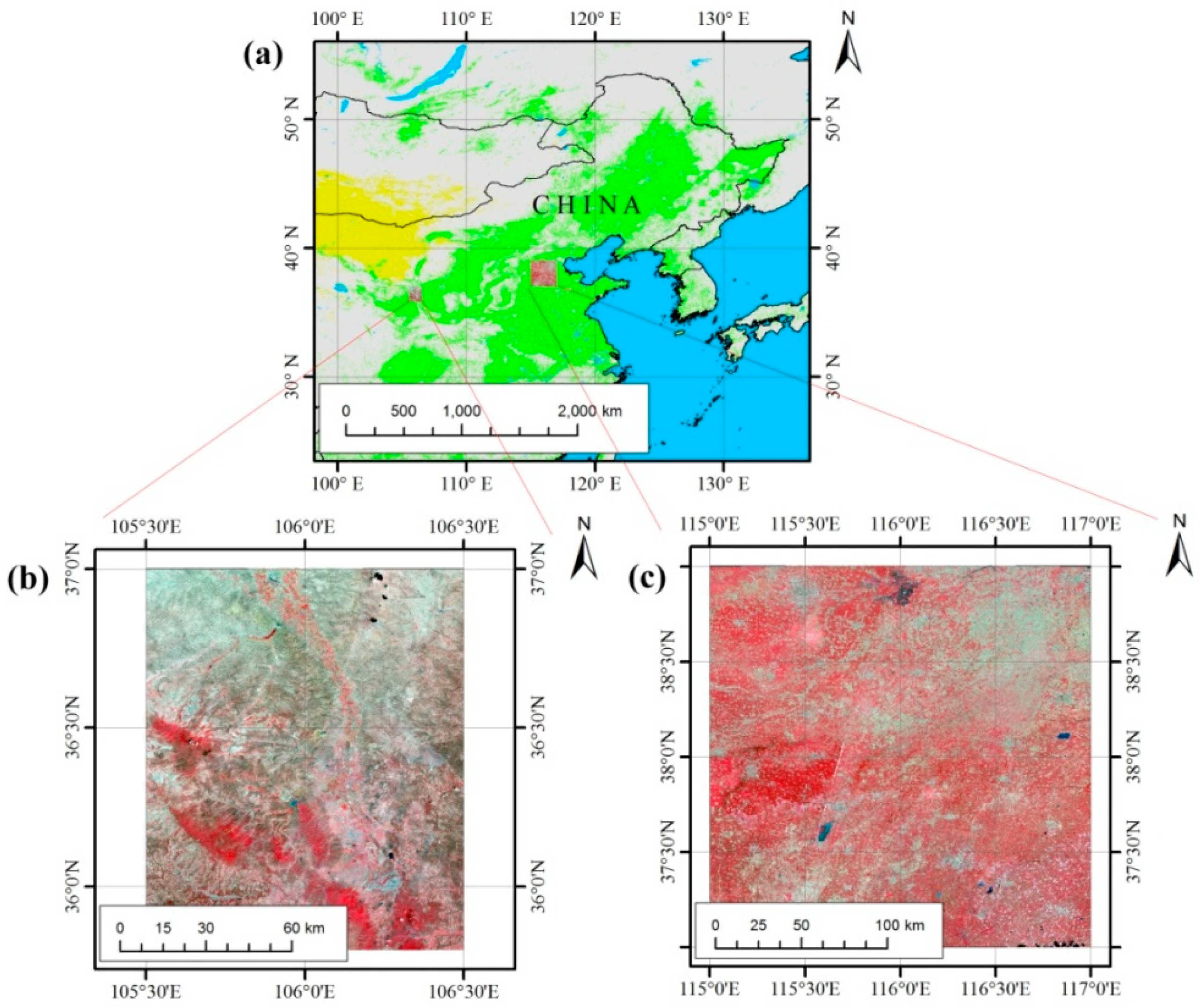
Two regions were analyzed in this study (Figure 1a). The first study region is located in Hengshui City (115°10’–116°34’ E, 37°03’–38°23’ N) of Hebei province (Figure 1c). This region has a warm temperate continental monsoon climate that is characterized by hot, rainy summers and cold, dry winters. Cropland is the dominant land cover/use type of this area [33]. The major crop types in the study region are winter wheat, summer maize, spring maize, and cotton fields; some of these vegetable fields have been widely mulched using white plastic film. The second study region is located in Guyuan city (105°30’–106°30’ E, 35°50’–37°0’ N) of Ningxia Hui Autonomous Region, China (Figure 1b). This region has a temperate semi-arid climate with limited precipitation, so that the crops require irrigation during the growing season; the crop fields are irrigated by groundwater or river water from canals. For fields without irrigation facilities, plastic mulch film has been utilized widely to save water in Guyuan [34]. As the most PML are covered with the white films, so that we only focus on the PML with white films in this study, the PML of other colors could lead to the change of their reflectance, and these PML are not considered in this study.

3. Data Sets

3.1. Sentinel-2 Data and Preprocessing

Sentinel-2 provides multi-spectral optical data (visible, near-infrared, shortwave infrared bands) at 10–20 m spatial resolution with a 5-day revisit frequency; such data have shown good potential to identify land cover and crop types [35,36]. In this study, we sourced all available Sentinel-2 top of atmosphere (TOA) reflectance data between April and October 2018 in both study regions for PML mapping. In Hengshui, we collected 235 images (tiles T48SWE, T48SWF, T48SXE and T48SXF); and in Guyuan, we collected 299 images (tiles T50SLG, T50SLH, T50SMG and T50SMH). The Sentinel-2 TOA reflectance data are freely available on the Google Earth Engine (GEE) platform as “COPERNICUS/S2” and we processed the data on GEE [37]. We just used the TOA reflectance in this study because only TOA reflectance of Sentinel-2 data is available on GEE platform. Emelyanova et al. [38] compared the performance between classification using TOA reflectance and surface reflectance (SR), and found that TOA reflectance and SR reflectance data generated similar classification results, and some indices (such as Normalized Difference Water Index) calculated from TOA and SR reflectance had high correlation. Therefore, although the use of TOA reflectance is not perfect, the classification result could be used to estimate the performance of the newly proposed workflow.

The data pre-processing contained several steps. We firstly used the Quality assurance (QA) band to mask the cloud pixels (pixels with a QA value equal to 0 are deemed non-cloud pixels). Next, 15-day image time-series were generated using the 15-day maximum composition for the 10 multi-spectral bands (blue, green, red, three red-edge, two NIR, and two SWIR bands) [39], and each 15-day composited image was defined as one time phase. The number of Sentinel-2 images we acquired in each 15-day period are shown in Table S1. Then, we acquired the 15-day image time series. All data were resampled to 20 m because the spatial resolution of the red-edge and SWIR bands is 20 m. Next, we used the 15-day image time series to calculate some indices, such as NDVI, PMLI, and also the new PML indices proposed in this study (Section 4.2.1). All features included in this study are shown in

Table 1. Features extracted from the Sentinel-2 images.

Bands/Indices	Equations
$\mathsf{\rho }\left(\mathrm{Blue}\right)$	Reflectance of Blue 3 band (B7 of Sentinel-2)
$\mathsf{\rho }\left(\mathrm{Green}\right)$	Reflectance of Green 3 band (B7 of Sentinel-2)
$\mathsf{\rho }\left(\mathrm{Red}\right)$	Reflectance of Red 3 band (B7 of Sentinel-2)
$\mathsf{\rho }\left(\mathrm{RE}1\right)$	Reflectance of Red-edge 1 band (B7 of Sentinel-2)
$\mathsf{\rho }\left(\mathrm{RE}2\right)$	Reflectance of Red-edge 2 band (B7 of Sentinel-2)
$\mathsf{\rho }\left(\mathrm{RE}3\right)$	Reflectance of Red-edge 3 band (B7 of Sentinel-2)
$\mathsf{\rho }\left(\mathrm{NIRn}\right)$	Reflectance of narrow NIR band (B8A of Sentinel-2)
$\mathsf{\rho }\left(\mathrm{NIRb}\right)$	Reflectance of board NIR band (B8 of Sentinel-2)
$\mathsf{\rho }\left(\mathrm{SWIR}1\right)$	Reflectance of SWIR 1 band (B11 of Sentinel-2)
$\mathsf{\rho }\left(\mathrm{SWIR}2\right)$	Reflectance of SWIR 2 band (B12 of Sentinel-2)
PMLI_NIR	Equation (1) in this study
PMLI_SWIR	Equation (2) in this study
PMLI_ND	Equation (3) in this study
PML index (PMLI)	$\frac{\mathsf{\rho }\left(\mathrm{Red}\right)-\mathsf{\rho }\left(\mathrm{SWIR}1\right)}{\mathsf{\rho }\left(\mathrm{Red}\right)+\mathsf{\rho }\left(\mathrm{SWIR}1\right)}$ [15]
Normalized Difference Vegetation Index (NDVI)	$\frac{\mathsf{\rho }\left(\mathrm{NIRn}\right)-\mathsf{\rho }\left(\mathrm{Red}\right)}{\mathsf{\rho }\left(\mathrm{NIRn}\right)+\mathsf{\rho }\left(\mathrm{Red}\right)}$ [40]
Normalized Difference Water Index (NDWI)	$\frac{\mathsf{\rho }\left(\mathrm{Green}\right)-\mathsf{\rho }\left(\mathrm{NIRn}\right)}{\mathsf{\rho }\left(\mathrm{Green}\right)+\mathsf{\rho }\left(\mathrm{NIRn}\right)}$ [41]

Note: $\mathsf{\rho }$ denotes multi-spectral band.

.

3.2. Ground Reference Data

The ground samples were collected during a field survey in 2018, and we went to HS three times (in late April, early May, and late June) and GY once (June) for field surveys. We took the GPS to the fields, recorded the coordinate of the fields and whether the fields are plastic-film covered or non-plastic-film covered. The samples we collected in the ground survey were characterized by large field sizes (larger than 30 × 30 m), and we only recorded the center point of each field. In HS, we only recorded plastic-film covered fields as we could only confirm the plastic-film covered fields were PML samples, and the bare land fields we surveyed during April and May could become PML fields. In June, the crop had grown up, so that we recorded both plastic-film covered (PML) and non-plastic-film covered (non-PML) fields, the non-PML contained non-PML crop fields (winter wheat/summer maize and maize fields), residential regions, and water. Then, all samples collected in April, May and the randomly selected one-third non-plastic-film covered samples collected in June were used as training samples. The plastic-film covered samples and the other two-third non-plastic-film covered samples collected in June were used as validation samples for HS. In GY, we only had the ground survey in June and collected PML and non-PML samples, and all these samples were used as validation samples for GY. The training samples were used to generate the rules for PML identification. Next, the rules were used to identify PML in both HS and GY, and validation samples in the two study regions were used to assess the classification accuracy in both study regions. The number of samples collected in HS and GY used as training/validation samples is shown in

Table 2. Number of samples collected for this study.

Time	Class	HS	GY
April	PML	128	0
May	PML	102	0
June	PML	176	201
	non-PML (a part of spring maize fields used for training)	146	0
	non-PML (used for validation)	252	254

.

4. Methods

4.1. Principle and Workflow

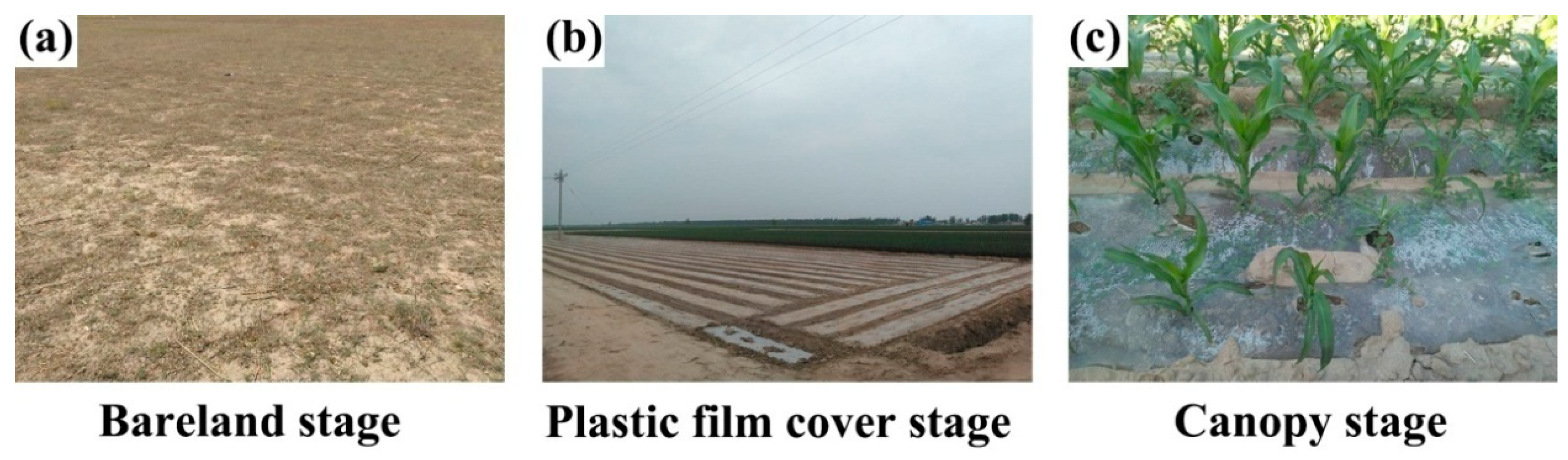
The status of the PML change during the growing season could be regarded as three stages: (1) bare land stage, (2) plastic-film-covered stage, and (3) canopy stage. In the bare land stage, the crops are sown and the fields are still bare land (Figure 2a). In the plastic-film-covered stage (Figure 2b), the fields are covered by plastic film and the plants have not grown yet. In this stage, the new plastic-film sheets are spread but the films gradually become soiled, so that plastic-covered fields could be separated from bare land before the plastic-film becomes soiled. In the canopy stage, the plants of both PML and non-PML have grown and the fields are covered by the canopy. In this stage, the PML could be discriminated from non-vegetation land, such as residential regions and water surface.

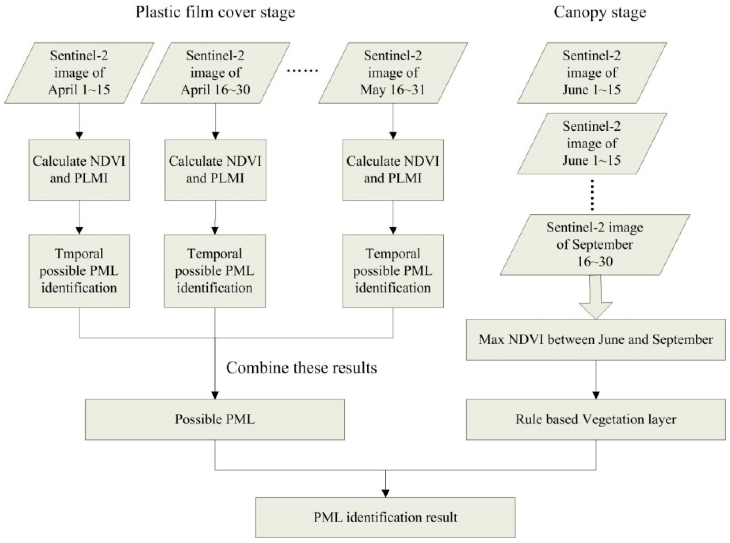
Therefore, we developed a new workflow for regional PML identification by merging PML layers of multiple temporal phases (MTPML) (Figure 3). Firstly, we proposed three new PML indices for bare land and PML discrimination based on the TOA reflectance of the optical spectral bands, and the indices were calculated for each 15-day composited image (Section 3.1) during the plastic-film-covered stage. Next, we generated a “temporal possible PML layer” for each temporal phase and then combined possible PML of all temporal phases together to generate the “possible PML layer.” Afterwards, we calculated the maximum NDVI during June and September, as most crops had high NDVI during this temporal period, therefore a rule-based method could be used to generate a “vegetation layer.” Finally, we combined the “possible PML layer” and the “vegetation layer” to generate the PML. As the training samples were only collected in HS, the rules used for PML mapping were generated from the training samples in HS, and the rules were applied in both study regions for PML identification.

4.2. Possible PML Layer Generation

4.2.1. New PML Indices

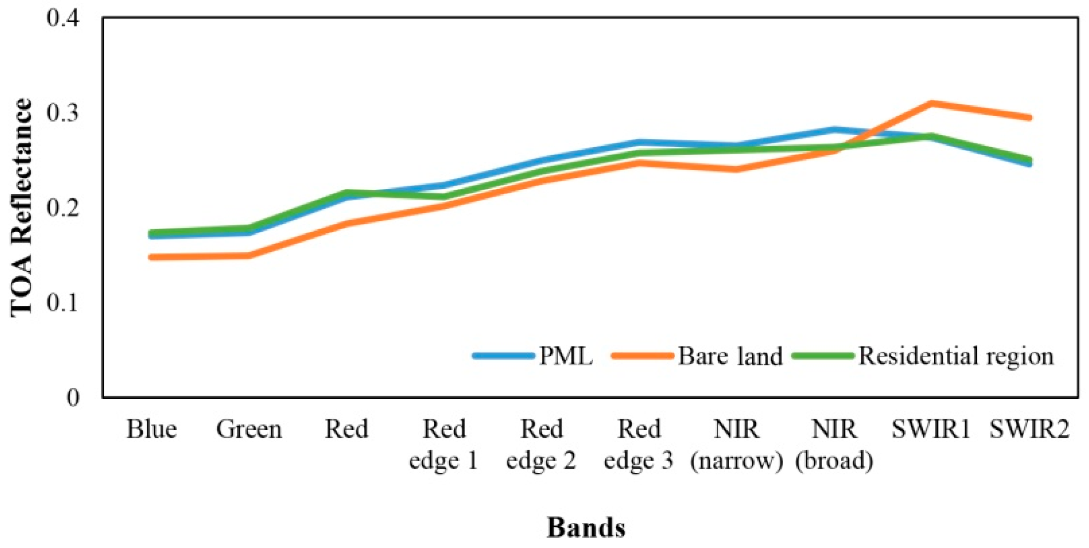
Existing studies have shown that PML can easily be separated from vegetation and water but can be confused with bare land and residential regions at the plastic film cover stage [15,18]. Therefore, we propose new indices for PML and bare land discrimination. Figure 4 shows typical spectral profiles of PML, bare land, and residential region in the plastic-film-covered stage. Generally, TOA reflectance of PML are higher than bare land in the visible, red-edge, and NIR bands. Furthermore, the TOA reflectance of PML are lower than bare land in SWIR1 and SWIR2 bands. This is because there is water content in the surface layers of PML, and the reflectance of wet soil is generally lower than dry soil in the two SWIR bands with band lengths between 1.3 and 2.5 μm [42]. Therefore, we proposed three new PMLIs to discriminate PML from bare land based on these characteristics. The TOA reflectance of PML and residential region were more similar at the plastic film cover stage, but at canopy stage, the plants in the PML had grown up and then PML could be easily discriminated from residential regions.

The new PML indices were proposed based on the spectral characters of the PML and bare land (Figure 4). As the NIR and red-edge bands had higher reflectance than the SWIR bands for PML pixels, we defined narrow NIR, broad NIR, and Red-edge 3 bands as “NIR” bands, and SWIR 1 and 2 bands as “SWIR” bands. We then calculated the sum of the NIR and SWIR bands and thus increased the difference in the NIR and SWIR bands between the PML and bare land. We subtracted the SWIR bands reflectance sum by the NIR bands reflectance sum, and the difference value (D-value) of PML samples was higher than the bare land samples. Next, this D-value was divided by the NIR reflectance sum, SWIR reflectance sum, and five band reflectance (both NIR and SWIR bands) sum. These three indices were named as PMLI with NIR bands (PMLI_NIR), PMLI with SWIR bands (PMLI_SWIR), and Normalized difference PMLI (PMLI_ND) (Equations (1), (2) and (3)).

$${\mathrm{PMLI}}_{\mathrm{NIR}}=\frac{\left(\mathsf{\rho }\left(\mathrm{NIRn}\right)+\mathsf{\rho }\left(\mathrm{NIRb}\right)+\mathsf{\rho }\left(\mathrm{RE}3\right)\right)-\left(\mathsf{\rho }\left(\mathrm{SWIR}1\right)+\mathsf{\rho }\left(\mathrm{SWIR}2\right)\right)}{\mathsf{\rho }\left(\mathrm{NIRn}\right)+\mathsf{\rho }\left(\mathrm{NIRb}\right)+\mathsf{\rho }\left(\mathrm{RE}3\right)},$$

(1)

$${\mathrm{PMLI}}_{\mathrm{SWIR}}=\frac{\left(\mathsf{\rho }\left(\mathrm{NIRn}\right)+\mathsf{\rho }\left(\mathrm{NIRb}\right)+\mathsf{\rho }\left(\mathrm{RE}3\right)\right)-\left(\mathsf{\rho }\left(\mathrm{SWIR}1\right)+\mathsf{\rho }\left(\mathrm{SWIR}2\right)\right)}{\mathsf{\rho }\left(\mathrm{SWIR}1\right)+\mathsf{\rho }\left(\mathrm{SWIR}2\right)},$$

(2)

$${\mathrm{PMLI}}_{\mathrm{ND}}=\frac{\left(\mathsf{\rho }\left(\mathrm{NIRn}\right)+\mathsf{\rho }\left(\mathrm{NIRb}\right)+\mathsf{\rho }\left(\mathrm{RE}3\right)\right)-\left(\mathsf{\rho }\left(\mathrm{SWIR}1\right)+\mathsf{\rho }\left(\mathrm{SWIR}2\right)\right)}{\mathsf{\rho }\left(\mathrm{NIRn}\right)+\mathsf{\rho }\left(\mathrm{NIRb}\right)+\mathsf{\rho }\left(\mathrm{RE}3\right)+\mathsf{\rho }\left(\mathrm{SWIR}1\right)+\mathsf{\rho }\left(\mathrm{SWIR}2\right)}.$$

(3)

4.2.2. Feature Separability and Importance Estimation

We used the Jeffries–Matusita (JM) distance and Gini index generated from the Random Forest algorithm to estimate the feature separability and importance for PML and bare land discrimination [19,26]. The JM distance between a pair of classes could be calculated by:

$$\mathrm{JM}\left({\mathrm{c}}_{\mathrm{i}},{\mathrm{c}}_{\mathrm{j}}\right)={{\displaystyle \int }}_{\mathrm{x}}^{}{\left(\sqrt{\mathrm{p}\left(\mathrm{x}|{\mathrm{c}}_{\mathrm{i}}\right)}-\sqrt{\mathrm{p}\left(\mathrm{x}|{\mathrm{c}}_{\mathrm{j}}\right)}\right)}^2\mathrm{dx},$$

(4)

where x denotes a span of feature series values, and ${\mathrm{c}}_{\mathrm{i}}$ and ${\mathrm{c}}_{\mathrm{j}}$ denote the two classes, and Equation (1) is commonly reduced to $\mathrm{JM}=2\left(1-{\mathrm{e}}^{-\mathrm{B}}\right)$ where

$$\mathrm{B}=\frac{1}{8}{\left({\mathsf{\mu }}_{\mathrm{i}}-{\mathsf{\mu }}_{\mathrm{j}}\right)}^{\mathrm{T}}{\left(\frac{{\mathrm{C}}_{\mathrm{i}}+{\mathrm{C}}_{\mathrm{j}}}{2}\right)}^{-1}\left({\mathsf{\mu }}_{\mathrm{i}}-{\mathsf{\mu }}_{\mathrm{j}}\right)+\frac{1}{2}\ln \left(\left|\frac{\left|{\mathrm{C}}_{\mathrm{i}}+{\mathrm{C}}_{\mathrm{j}}\right|}{2\sqrt{\left|{\mathrm{C}}_{\mathrm{i}}\right|\times \left|{\mathrm{C}}_{\mathrm{j}}\right|}}\right|\right),$$

(5)

and ${\mathrm{C}}_{\mathrm{i}}$ and ${\mathrm{C}}_{\mathrm{j}}$ are the covariance matrixes of class i and j, and $\left|{\mathrm{C}}_{\mathrm{i}}\right|$ and $\left|{\mathrm{C}}_{\mathrm{j}}\right|$ are the determinants of ${\mathrm{C}}_{\mathrm{i}}$ and ${\mathrm{C}}_{\mathrm{j}}$, respectively. The JM distance ranges from 0 to 2 and a large value indicates a high level of separability between two classes.

The Random Forest (RF) algorithm is an ensemble machine learning technique that combines multiple classification trees and has been widely used for image classification [43]. Each tree is constructed using two-thirds of the training records and the remaining records are used for a test classification with an “out-of-bag error.” During the training procedure of RF, every time a variable node is split, the Gini impurity criterion for the descendent nodes is less than that of the parent node. The importance score for each individual variable is the sum of the Gini decreases over all trees in the classification forest. In this research, the Gini importance score was obtained using the RandomForest package for R [44]. The number of trees in the ensemble was set to 1000 to allow convergence of the error statistic, and the number of features to split the nodes in the trees was set to the square root of the total number of input features.

In this study, both JM distance and Gini importance score were used to estimate the potential of each feature for PML and bare land discrimination at the plastic-film cover stage. As we collected 128 and 102 PML samples in April and May, we extracted the 10 multi-spectral bands and the five indices (Table 1) from the April 16~30 and May 16~31 image using the corresponding samples collected in April and May, then we visually interpreted bare land samples from the non-PML samples in the training sample dataset (Table 2), and used these samples to extracted the 15 features (Table 1) from April 16~30 and May 16~31 images. Next, we calculated the JM distance and Gini importance score of each feature for separating PML and bare land.

4.2.3. Possible PML Layer Generation

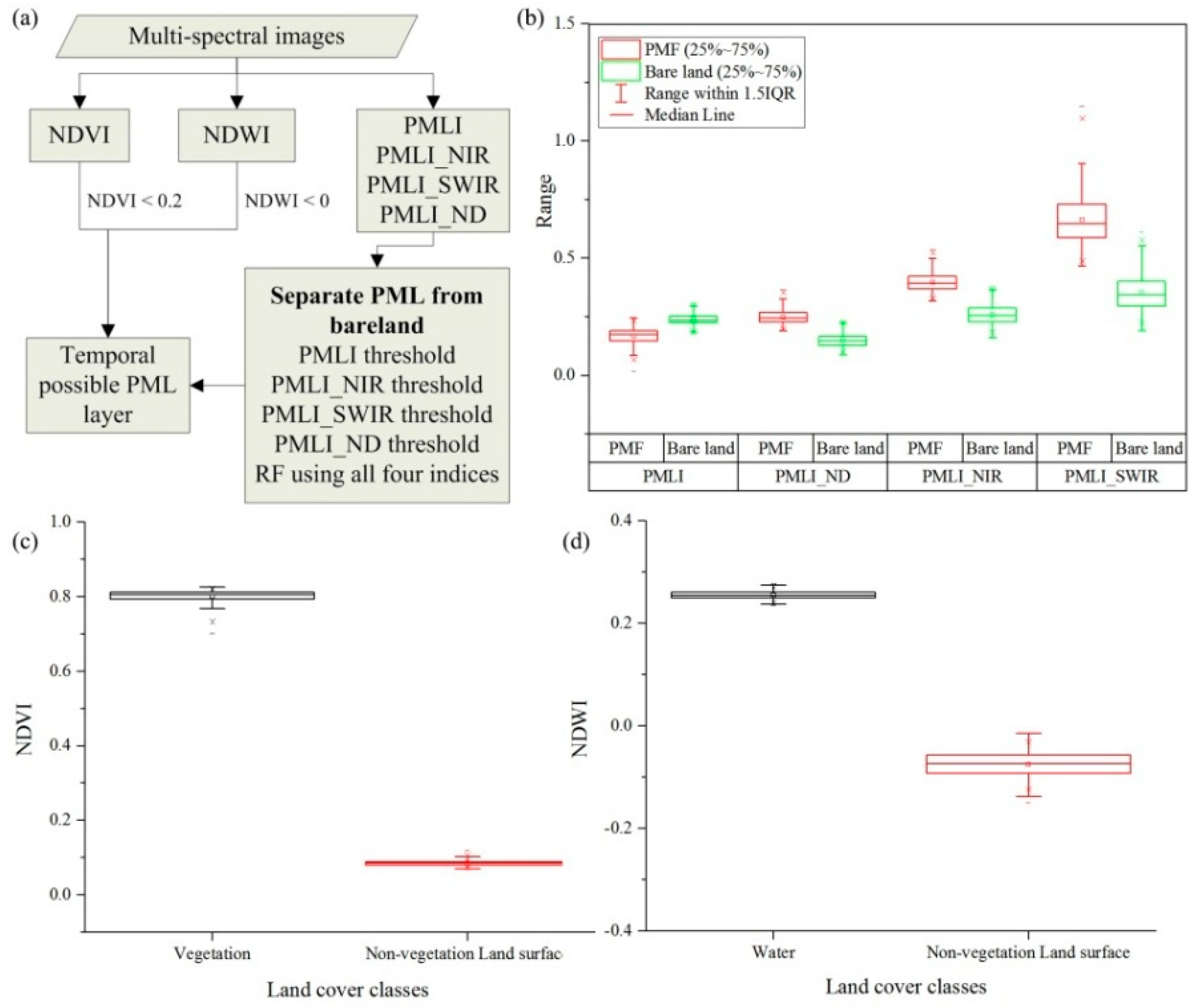
As the plastic-film-covered stages were mainly in April and May, we used the 15-day composited images of four time phases (April 1–15 and 16–30, and May 1–15 and 16–31) to generate the possible PML layer, and the “temporal possible PML layer” for each temporal phase was generated based on the NDVI, NDWI, and PMLIs using a decision tree (Figure 5a). NDVI and NDWI were firstly used to exclude surface water and vegetation. We visually interpreted 1500 samples for water, vegetation, and non-vegetation land surface, and used these samples to define the threshold for the vegetation mask and water mask, and the threshold of NDVI and NDWI were set as 0.2 and 0 (Figure 5c,d). Next, we used five approaches to discriminate bare land from PML, the five approaches were threshold rule-based methods using PMLI_NIR, PMLI_SWIR, PMLI_ND, PMLI; and the RF classification method using all these four indices. Figure 5b shows the range and average value of the PMLI_NIR, PMLI_SWIR, and PMLI_ND values for the training PML and bare land samples (Table 2). For PMLI_NIR, PMLI_SWIR, and PMLI_ND, the indices value of PML were higher than bare land, so that the thresholds were calculated by subtracting the standard deviation of the PML samples from the mean value, and the thresholds were set as 0.36 for PMLI_NIR, 0.55 for PMLI_SWIR, 0.22 for PMLI_ND, and pixels with indices higher than the threshold were labeled as “temporal possible PML.” For PMLI, the index value of PML was lower than bare land, and the threshold was calculated by adding the standard deviation of the PML samples to the mean value, which was 0.2. Pixels with PMLI lower than the 0.2 were labeled as “temporal possible PML.” The last approach was using RF to separate PML and bare land. All four PML indices were used as input features. The training samples (Table 2) collected in HS were used to train the RF classifier. The RF classifier was then used to separate PML from bare land for the image from each 15-day temporal phase. The RF algorithm was implemented using the RandomForest package in R (similar to Section 4.2.2). For each approach, we finally calculated the union of PML from the four “temporal possible PML layers” and generated the possible PML layers.

4.3. Vegetation Layer and PML Map Generation

In the plastic-film-covered stage, the PML is confused with some other land cover types, such as residential regions, stone, and greenhouses; thus, the possible PML layer we generated in Section 4.2 might still contain some non-cropland pixels. Therefore, we excluded the non-cropland pixels from the “possible PML layer” using a vegetation layer. Generally, the cropland fields had high vegetation fraction during June and September, so that we calculated the maximum NDVI in this temporal period. As the max NDVI for cropland cannot be lower than 0.4 in most cases [45], we used 0.4 as the threshold to generate the vegetation layer. Finally, we used both the possible PML layer and the vegetation layer to generate the PML distribution. Pixels in both layers were classified as PML.

In addition, we used the supervised method (named as SUPML in this study) to identify PML and to compare the results with the five MTPML results. As recommended by Hasituya and Chen [18], multi-spectral and NDVI bands of all 15-day composited images between April and May were used. RF was utilized as a classifier and the training samples were used to train the classifier. We did not use this approach to identify PML in GY because we only collected training samples in HS.

4.4. Accuracy Assessment

We used both accuracy and statistical metrics to verify and compare the PML identification results generated by different approaches (MTPML with PMLI, MTPML with PMLI_NIR, MTPML with PMLI_SWIR, MTPML with PMLI_ND, MTPML with RF and SUPML). Firstly, metrics (producer’s accuracy (PA), user’s accuracy (UA), overall accuracy (OA), and Kappa coefficient) from the confusion matrix were used to assess the PML maps generated in both study regions [46]. All these accuracy metrics were calculated from the validation samples. In addition, we applied McNemar’s test to evaluate the pair-wise statistical significance of the difference between PML generated by different approaches [47]. McNemar’s test is a non-parametric test based on the standardized normal test statistic, as in Equation (6):

$$\mathrm{Z}=\frac{{\mathrm{f}}_{12}-{\mathrm{f}}_{21}}{\sqrt{{\mathrm{f}}_{12}+{\mathrm{f}}_{21}}},$$

(6)

where ${\mathrm{f}}_{12}$ is the number of samples that are correctly classified by classifier 1 and incorrectly classified by classifier 2. We defined three cases of differences in the accuracy between classifier 1 and classifier 2 according to McNemar’s test:

• No significance between classifiers 1 and 2 (N): −1.96 < Z < 1.96.
• Positive significance (classifier 1 has higher accuracy than classifier 2) (S+): Z > 1.96.
• Negative significance (classifier 1 has lower accuracy than classifier 2) (S-): Z < −1.96.

5. Results and Discussion

5.1. Feature Separability and Importance for Bare Land and PML Discrimination

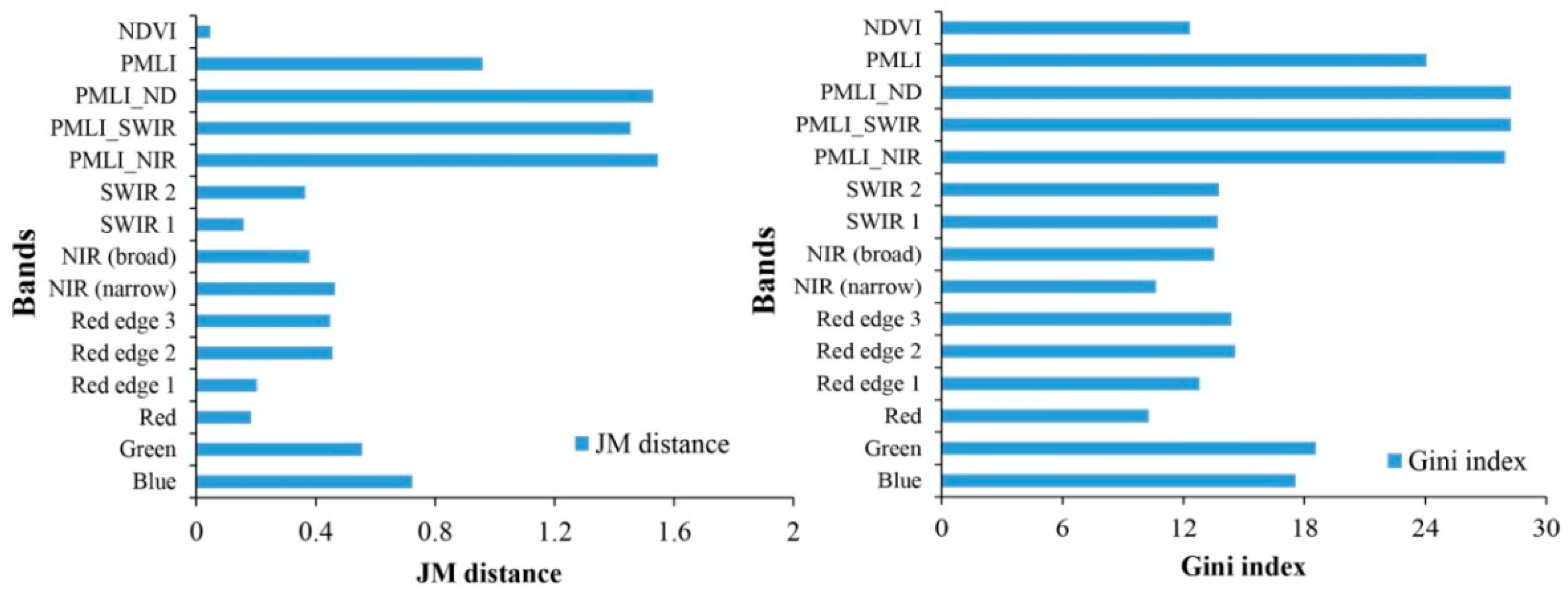
We used the JM distance and Gini index to estimate the separability and feature importance of each feature for PML and bare land discrimination. Figure 6 shows that the three new PML indices (PMLI_NIR, PMLI_SWIR, and PMLI_ND) had good separability and a high importance score. The JM distance of PMLI_NIR, PMLI_SWIR, and PMLI_ND were around 1.5 and the Gini score of these three bands were higher than 28. Separability and Gini importance of PMLI were lower than the newly proposed PML indices as the JM distance of PMLI was 0.9 and the Gini importance score was about 24. NDVI and multi-spectral bands led to a poor performance when discriminating bare land from PML. The JM distances of these bands were lower than 0.8 and the Gini importance scores were lower than 18, which were both significantly lower than the three new PML indices. Based on this result, we used the four PML indices (PMLI, PMLI_NIR, PMMLI_SWIR, and PMLI_ND) to generate “possible PML layers” (Section 4.2.3).

5.2. PML Mapping Accuracy Assessment

We used the validation samples (Table 2) to verify the classification accuracy in both study regions. Results from Hengshui (

Table 3. Classification accuracies assessment in HS and GY.

		OA(%)	Kappa	PA of PML (%)	UA of PML (%)	PA of non-PML(%)	PA of non-PML(%)
In HS
MTPML	PMLI	86.68	0.7266	85.8	82.51	87.30	89.80
	PMLI_NIR	90.19	0.7942	82.95	92.41	95.24	88.89
	PMLI_SWIR	89.25	0.7814	92.05	83.51	87.30	94.02
	PMLI_ND	88.08	0.7499	80.11	89.81	93.65	87.08
	RF	91.59	0.8266	90.34	89.33	92.46	93.20
SUPML		83.64	0.6581	76.14	82.72	88.89	84.21
In GY
MTPML	PMLI	83.74	0.6766	91.04	76.57	77.95	91.67
	PMLI_NIR	85.49	0.7062	84.08	83.25	86.61	87.30
	PMLI_SWIR	85.27	0.7038	87.06	81.02	83.86	89.12
	PMLI_ND	85.27	0.7019	84.08	82.84	86.22	87.25
	RF	87.47	0.7456	85.07	86.36	89.37	88.33

Notes: OA—overall accuracy; PA—producer´s accuracy; UA—user´s accuracy; “MTPML” denotes that the PML map was generated using the MTPML workflow proposed in this study (Section 4.1), “SUPML” denotes that the PML map was generated using the supervised RF (Section 4.3).

) show that the MTPML workflow proposed in this study led to higher PML identification accuracy than the supervised method. The low accuracy of SUPML was mainly due to the detectable period changing among different fields. For example, some PML fields were detectable during April 1–15 while other fields were detectable during May 1–15, and the temporal character of these fields was different even though these fields were all PML. However, the MTPML workflow proposed in this study could overcome this drawback because “temporal possible PML layer” was identified in each temporal period, we then calculated the union of all these temporal results between April and May. Therefore, this merged “possible PML layer” contained PML detected in each temporal period.

Among the five approaches used for the MTPML workflow, the RF approach had the highest PML identification accuracies in both study regions, followed by PMLI_SWIR and PLMI_NIR. The classification accuracies of PMLI were the lowest among the five approaches. The high accuracy of the RF approach was reasonable because this approach considered all four PML indices. The four threshold-based approaches were easier to conduct and the accuracies of the approaches using PMLI_SWIR and PMLI_NIR thresholds were slightly lower (1%–2%) than the RF approach. The PMLI_SWIR approach had the highest accuracies among the four PML indices because the reflectance of the SWIR bands was used as a denominator (Equation (2)), which further increased the difference between PML and bare land. Furthermore, the RF classifier and threshold rules generated in HS might potentially be used to identify PML in other study regions as they achieved good PML identification accuracies in GY.

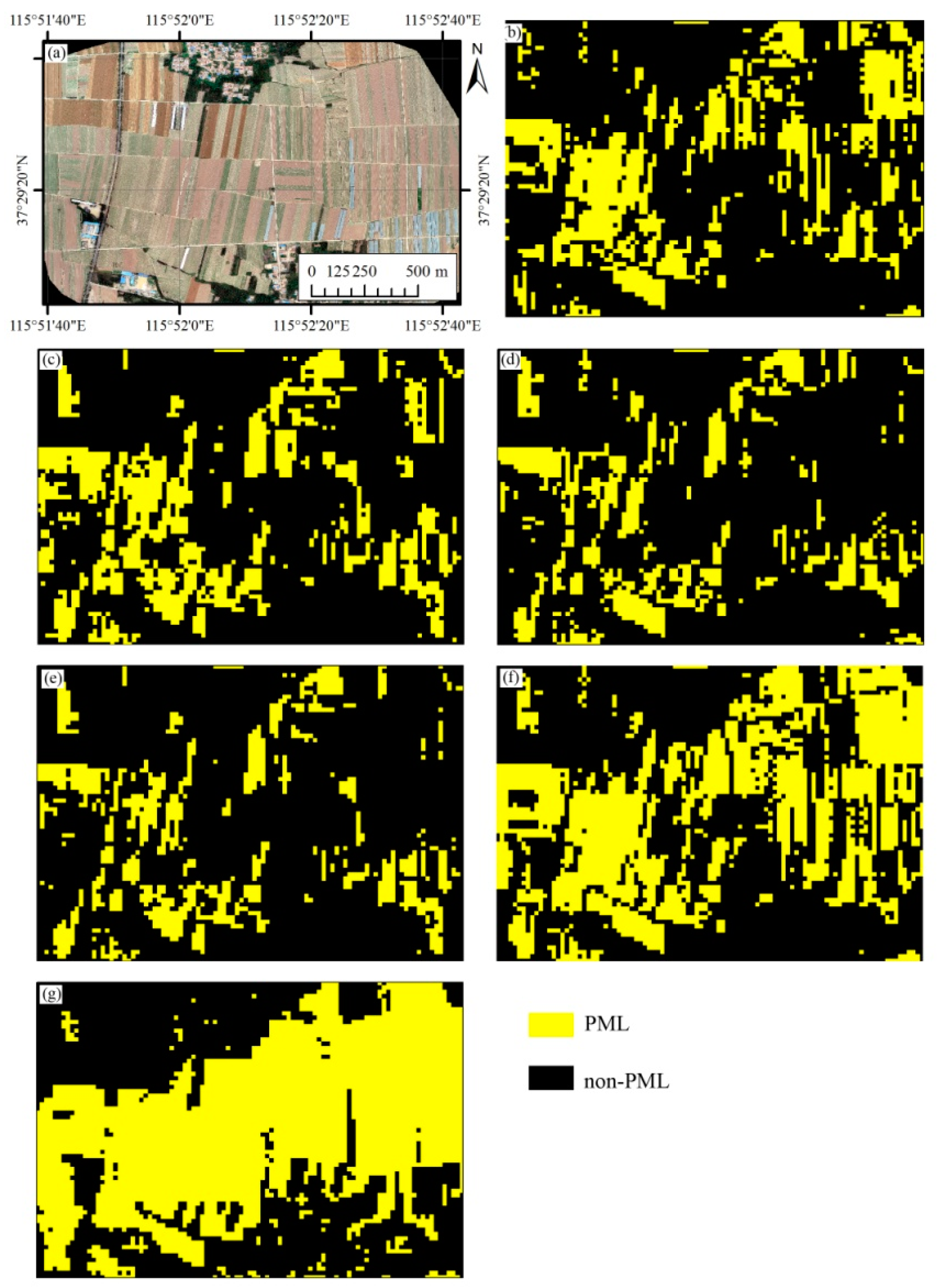
We used several subset regions of the two study regions to visually compare the PML identification results of the different approaches. In HS, we acquired Unmanned Aerial Vehicle (UAV) images (Figure 7a and Figure 8a) and we used these UAV images to compare the PML identification results because most plastic films were spread in April and May. In the first subset region of HS (Figure 7), the white patterns of the UAV images (Figure 7a) were PML, and the PML covered the majority of the sub-region. Among all the approaches used for PML mapping, the PML identified using the MTPML workflow with the RF classifier had the highest consistency with the UAV images. SUPML had the lowest accuracy as the non-PML was misclassified as PML. Results generated from MTPML with PMLI_NIR, PMLI_SWIR, and PMLI_ND thresholds had similar classification accuracies and they misclassified some PML pixels as non-PML. In the second sub-region (Figure 8), the light-green patterns of UAV images (Figure 8a) are the PML at the canopy stage and the white patterns are the PML at the plastic-film-covered stage. Among all the PML mapping approaches, SUPML misclassified the most non-PML samples as PML and MTPML with RF also misclassifying some non-PML samples as PML. MTPML with PMLI_NIR, PMLISWIR, and PMLI_ND thresholds had similar results, which were highly consistent with the UAV images.

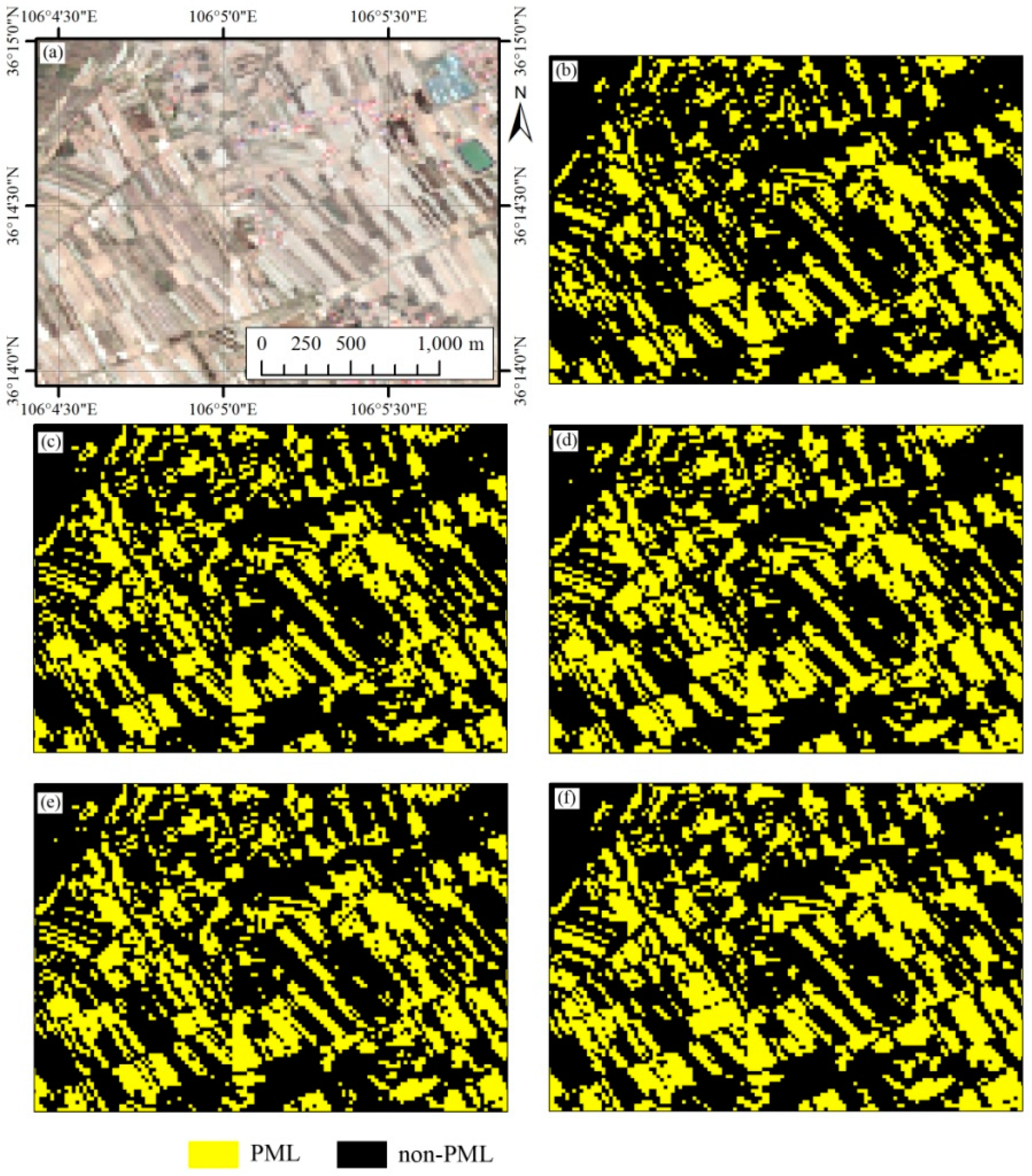
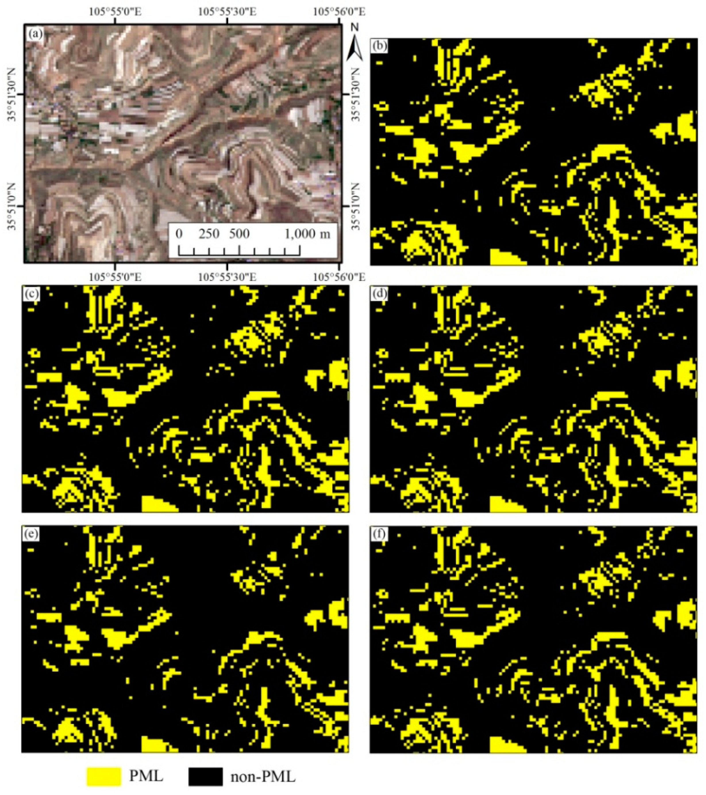
We selected two sub-regions in GY for wall to wall PML identification results comparison. The first sub-region is located in the plain region and the second is located in the mountain region. As we did not acquire UAV images during our field trip, we used the Sentinel-2 images composited during June 1–15 as the reference image. The white patterns in the reference images (Figure 9a and Figure 10a) were PML. Generally, the PML results generated from the five approaches were consistent with the reference images in both the plain and mountain regions (Figure 9a and Figure 10a), except for the PML results using the PMLI threshold, which were more fragmented in both sub-regions.

5.3. Statistical Comparison

We used McNemar’s test to compare the classification performances of the six approaches (

Table 4. McNemar’s test result in HS.

		MTPML
		RF	PMLI_NIR	PMLI_SWIR	PMLI_ND	PMLI
MTPML	PMLI_NIR	1.34 (N)
	PMLI_SWIR	1.71 (N)	0.59 (N)
	PMLI_ND	2.79 (S+)	1.48 (N)	0.78 (N)
	PMLI	3.13 (S+)	2.02 (S+)	3.32 (S+)	1.06 (N)
SUPML		3.71 (S+)	3.02 (S+)	2.31 (S+)	1.93 (N)	1.20 (N)

and

Table 5. McNemar’s test result in GY.

		MTPML
		RF	PMLI_NIR	PMLI_SWIR	PMLI_ND
MTPML	PMLI_NIR	1.41 (N)
	PMLI_SWIR	1.51 (N)	0.28 (N)
	PMLI_ND	1.54 (N)	1.00 (N)	0.00 (N)
	PMLI	2.65 (S+)	1.15 (N)	1.04 (N)	1.00 (N)

). In HS, the MTPML workflow significantly outperformed SUPML as the McNemar’s test result between MTPML RF and SUPML was 3.71 (S+). Among the five approaches used for the MTPML workflow, the PMLI threshold approach had the lowest accuracy as McNemar’s test results between RF and PMLI, PMLI_NIR and PMLI, PMLI_SWIR and PMLI in HS, and PMLI_NIR and PMLI in GY were S+. The RF approach outperformed the PMLI_NIR and PMLI_SWIR threshold approaches, but the improvement was not significant, which indicated that the simple threshold-based approaches in the MTPML workflow could generate accurate PML maps. Generally, all the results of the classification accuracy assessment, wall to wall comparison of the approaches, and McNemar’s test show that the MTPML workflow outperformed the supervised classification methods for PML identification. The RF approaches had the best performance in the MTPML workflow. The PMLI_NIR and PMLI_SWIR threshold approaches proposed in this study can be implemented simply and the PML identification performances were only slightly lower than the RF approach.

5.4. Advantages and Limitations

This study proposes a new workflow, MTPML, for PML identification using multi-temporal Sentinel-2 images and proposes three new PML indices to discriminate PML and bare land. Compared with the existing PML identification literature using a single-temporal image or supervised classification methods, the MTPML workflow and PML indices proposed in this study have several advantages.

(1) The MTPML workflow is specially designed to identify PML as the detectable temporal phases (plastic film stage) of PML change among the crop fields. The MTPML outperforms supervised classification methods when RF is used in both workflows as the classifier.

(2) Compared with the PMLI proposed for detecting PML, the three new PML indices (PMLI_NIR, PMLI_SWIR, and PMLI_ND) proposed in this study are designed to discriminate PML from bare land, and the reflectance of multiple NIR band SWIR bands are combined to increase the separating capability between bare land and PML. Feature separability, importance, and PML identification accuracies show that the PMLI_NIR and PMLI_SWIR outperform PMLI. The PMLI_SWIR approach has the best performance because using the SWIR reflectance as the denominator further enlarge the discrimination of the index.

(3) We propose a threshold-based method for each temporal phase. This method is easily implemented, and the PML identification performance of the threshold-based methods are only slightly lower than the RF approach.

(4) It is notable that the PML identification rules and RF classifier are generated in HS and in GY and that no training samples are used. This proves that the rules generated in this study have good potential for white PML identification in other regions.

However, there are still some drawbacks of PML mapping using the MTPML workflow.

(1) The data availability and preprocessing quality—although the temporal resolution of Sentinel-2 data is five days, the “data missing” problem still exists in the 15-day composited image time series [36]; therefore, if we cannot acquire the image during the detectable temporal phases, the PML pixels may be omitted. Furthermore, the quality of the image preprocessing may lead to PML identification uncertainty because the cloud pixels will be identified as PML if the cloud-mask fails to remove these pixels.

(2) The threshold used for PML and bare land discrimination—the thresholds for identifying PML are calculated using the average and standard deviation of the PML samples, thus, the thresholds of the PML indices calculated in HS could be used for PML mapping in GY. However, the thresholds may still change in other study regions with different soil types, soil moisture, and soil organic matter content. Therefore, the rules (and particularly the thresholds) used in this study need to be further evaluated for other regions.

6. Conclusions

This study proposes a new workflow (MTPML) for PML identification, and the performance of the threshold-based approaches using three new PML indices with MTPML are tested. The experiments are carried out in two study regions with different climate and soil types and reach the following conclusions:

(1) The MTPML workflow proposed in this paper identifies PML by merging PML identified in each temporal phase. The MTPML provides a solution to the problem that the detectable temporal phase of PML changes among fields. MTPML show good potential to identify PML because the identification accuracies of MTPML are 3%–5% higher than supervised classification when using RF as the classifier.

(2) This study proposes three PML indices (PMLI_NIR, PMLI_SWIR, and PMLI_ND) for separating bare land from PML. All these indices have higher separability and importance than the multi-spectral bands and the existing PMLI. In addition, when using the MUPML workflow to identify PML, the threshold-based PMLI_SWIR approach has best PML identification performance (OA equal to 89.25% and 85.27% in HS and GY) among the four threshold-based approaches. The accuracy is only slightly lower than that of the RF approach.

(3) The PML identification models based on MTPML are generated using training samples in HS, and these models have good potential to generate PML maps in GY (accuracies higher than 85%), which indicates that the rules proposed in this study have the potential to identify PML in other regions.

We recommend using the MTPML workflow with the PMLI_SWIR approach for regional PML mapping because the threshold-based PMLI_SW approach is easy to implement, and this approach has good PML identification accuracy. The threshold of this approach should be further evaluated in other regions to reduce the PML identification uncertainty caused by different soil types, moisture, and organic matter content.

References

- Yang, Y.; Zhou, X.; Yang, Y.; Bi, S.; Yang, X.; Liu, D.L. Evaluating water-saving efficiency of plastic mulching in northwest china using remote sensing and sebal. Agric. Water Manag. 2018, 209, 240–248. [Google Scholar] [CrossRef]
- Hasituya; Chen, Z.; Li, F.; Hongmei. Mapping plastic-mulched farmland with c-band full polarization sar remote sensing data. Remote Sens. 2017, 9, 1264. [Google Scholar] [CrossRef]
- Bai, L.T.; Hai, J.B.; Han, Q.F.; Jia, Z.K. Effects of mulching with different kinds of plastic film on growth and water use efficiency of winter wheat in weibei highland. Agric. Res. Arid Areas 2010, 28, 135–136. [Google Scholar]
- Yu, Y.-Y.; Turner, N.C.; Gong, Y.-H.; Li, F.-M.; Fang, C.; Ge, L.-J.; Ye, J.-S. Benefits and limitations to straw- and plastic-film mulch on maize yield and water use efficiency: A meta-analysis across hydrothermal gradients. Eur. J. Agron. 2018, 99, 138–147. [Google Scholar] [CrossRef]
- Li, H.; Yang, X.; Chen, H.; Cui, Q.; Yuan, G.; Han, X.; Wei, C.; Zhang, Y.; Ma, J.; Zhang, X. Water requirement characteristics and the optimal irrigation schedule for the growth, yield, and fruit quality of watermelon under plastic film mulching. Sci. Hortic. 2018, 241, 74–82. [Google Scholar] [CrossRef]
- Qin, X.; Li, Y.; Han, Y.; Hu, Y.; Li, Y.; Wen, X.; Liao, Y.; Siddique, K.H.M. Ridge-furrow mulching with black plastic film improves maize yield more than white plastic film in dry areas with adequate accumulated temperature. Agric. Forest Meteorol. 2018, 262, 206–214. [Google Scholar] [CrossRef]
- Zhang, Y.-L.; Feng, S.-Y.; Wang, F.-X.; Binley, A. Simulation of soil water flow and heat transport in drip irrigated potato field with raised beds and full plastic-film mulch in a semiarid area. Agric. Water Manag. 2018, 209, 178–187. [Google Scholar] [CrossRef] [Green Version]
- Chae, Y.; An, Y.-J. Current research trends on plastic pollution and ecological impacts on the soil ecosystem: A review. Environ. Pollut. 2018, 240, 387–395. [Google Scholar] [CrossRef]
- Yu, Y.; Ji, H.; Zhao, C. Evaluation of the effects of plastic mulching and nitrapyrin on nitrous oxide emissions and economic parameters in an arid agricultural field. Geoderma 2018, 324, 98–108. [Google Scholar] [CrossRef]
- Wang, Q.; Zhang, H.; Liao, G.-T.; Lan, T.; Gao, X.-S.; Qiao, S.-B.; Yao, X.-Z. Spatial and temporal variation characteristics of the main agricultural inputs in sichuan province and the influencing factors. J. Ecol. Rural Environ. 2018, 34, 717–725. [Google Scholar]
- Yang, X.M.; Bento, C.P.M.; Chen, H.; Zhang, H.M.; Xue, S.; Lwanga, E.H.; Zomer, P.; Ritsema, C.J.; Geissen, V. Influence of microplastic addition on glyphosate decay and soil microbial activities in Chinese loess soil. Environ. Pollut. 2018, 242, 338–347. [Google Scholar] [CrossRef] [PubMed]
- Gong, P.; Wang, J.; Yu, L.; Zhao, Y.C.; Zhao, Y.Y.; Liang, L.; Niu, Z.G.; Huang, X.M.; Fu, H.H.; Liu, S.; et al. Finer resolution observation and monitoring of global land cover: First mapping results with landsat tm and etm+ data. Int. J. Remote Sens. 2013, 34, 2607–2654. [Google Scholar] [CrossRef]
- Xiong, J.; Thenkabail, P.S.; Tilton, J.C.; Gumma, M.K.; Teluguntla, P.; Oliphant, A.; Congalton, R.G.; Yadav, K.; Gorelick, N. Nominal 30-m cropland extent map of continental africa by integrating pixel-based and object-based algorithms using sentinel-2 and landsat-8 data on google earth engine. Remote Sens. 2017, 9, 1065. [Google Scholar] [CrossRef]
- Yang, D.; Chen, J.; Zhou, Y.; Chen, X.; Chen, X.; Cao, X. Mapping plastic greenhouse with medium spatial resolution satellite data: Development of a new spectral index. ISPRS J. Photogramm. Remote Sens. 2017, 128, 47–60. [Google Scholar] [CrossRef]
- Lu, L.; Di, L.; Ye, Y. A decision-tree classifier for extracting transparent plastic-mulched landcover from landsat-5 tm images. IEEE J. Sel. Top. Appl. Earth Obs. Remote Sens. 2014, 7, 4548–4558. [Google Scholar] [CrossRef]
- Novelli, A.; Aguilar, M.A.; Nemmaoui, A.; Aguilar, F.J.; Tarantino, E. Performance evaluation of object based greenhouse detection from sentinel-2 msi and landsat 8 oli data: A case study from Almería (Spain). Int. J. Appl. Earth Obs. Geoinf. 2016, 52, 403–411. [Google Scholar] [CrossRef]
- Aguilar, M.; Nemmaoui, A.; Novelli, A.; Aguilar, F.; García Lorca, A. Object-based greenhouse mapping using very high resolution satellite data and landsat 8 time series. Remote Sens. 2016, 8, 513. [Google Scholar] [CrossRef]
- Hasituya; Chen, Z. Mapping plastic-mulched farmland with multi-temporal landsat-8 data. Remote Sens. 2017, 9, 557. [Google Scholar] [CrossRef]
- Breiman, L. Random forests. Mach. Learn. 2001, 45, 5–32. [Google Scholar] [CrossRef]
- Mountrakis, G.; Im, J.; Ogole, C. Support vector machines in remote sensing: A review. ISPRS J. Photogramm. Remote Sens. 2011, 66, 247–259. [Google Scholar] [CrossRef]
- Lu, L.; Hang, D.; Di, L. Threshold model for detecting transparent plastic-mulched landcover using moderate-resolution imaging spectroradiometer time series data: A case study in southern Xinjiang, China. J. Appl. Remote Sens. 2015, 9, 097094. [Google Scholar] [CrossRef]
- Lu, L.; Tao, Y.; Di, L. Object-based plastic-mulched landcover extraction using integrated sentinel-1 and sentinel-2 data. Remote Sens. 2018, 10, 1820. [Google Scholar] [CrossRef]
- Massey, F.J. The Kolmogorov-Smirnov test for goodness of fit. J. Am. Stat. Assoc. 2012, 46, 68–78. [Google Scholar] [CrossRef]
- Mohammadimanesh, F.; Salehi, B.; Mahdianpari, M.; Brisco, B.; Gill, E. Full and simulated compact polarimetry sar responses to canadian wetlands: Separability analysis and classification. Remote Sens. 2019, 11, 516. [Google Scholar] [CrossRef]
- Hao, P.Y.; Zhan, Y.L.; Wang, L.; Niu, Z.; Shakir, M. Feature selection of time series modis data for early crop classification using random forest: A case study in Kansas, USA. Remote Sens. 2015, 7, 5347–5369. [Google Scholar] [CrossRef]
- Murakami, T.; Ogawa, S.; Ishitsuka, N.; Kumagai, K.; Saito, G. Crop discrimination with multitemporal SPOT/HRV data in the Saga Plains, Japan. Int. J. Remote Sens. 2001, 22, 1335–1348. [Google Scholar] [CrossRef]
- Wang, Y.; Qi, Q.; Ying, L. Unsupervised segmentation evaluation using area-weighted variance and Jeffries-Matusita distance for remote sensing images. Remote Sens. 2018, 10, 1193. [Google Scholar] [CrossRef]
- Jia, Y.; Yong, G.; Feng, L.; Xian, G.; Li, X. Urban land use mapping by combining remote sensing imagery and mobile phone positioning data. Remote Sens. 2018, 10, 446. [Google Scholar] [CrossRef]
- Hao, P.; Löw, F.; Biradar, C. Annual cropland mapping using reference landsat time series—A case study in central asia. Remote Sens. 2018, 10, 2057. [Google Scholar] [CrossRef]
- Low, F.; Michel, U.; Dech, S.; Conrad, C. Impact of feature selection on the accuracy and spatial uncertainty of per-field crop classification using support vector machines. ISPRS J. Photogramm. Remote Sens. 2013, 85, 102–119. [Google Scholar] [CrossRef]
- Wardlow, B.D.; Egbert, S.L. Large-area crop mapping using time-series MODIS 250 m NDVI data: An assessment for the U.S. Central Great Plains. Remote Sens. Environ. 2008, 112, 1096–1116. [Google Scholar] [CrossRef]
- ESA Sentinel-2 for Agriculture. Available online: http://www.esa-sen2agri.org/SitePages/sentinel2.aspx (accessed on 4 June 2019).
- Liu, H.; Guo, H.; Yang, L.; Wu, L.; Li, F.; Li, S.; Ni, P.; Liang, X. Occurrence and formation of high fluoride groundwater in the Hengshui area of the North China Plain. Environ. Earth Sci. 2015, 74, 2329–2340. [Google Scholar] [CrossRef]
- Hasituya; Chen, Z.; Wang, L.; Liu, J. Selecting appropriate spatial scale for mapping plastic-mulched farmland with satellite remote sensing imagery. Remote Sens. 2017, 9, 265. [Google Scholar] [CrossRef]
- Belgiu, M.; Csillik, O. Sentinel-2 cropland mapping using pixel-based and object-based time-weighted dynamic time warping analysis. Remote Sens. Environ. 2018, 204, 509–523. [Google Scholar] [CrossRef]
- Hao, P.; Tang, H.; Chen, Z.; Liu, Z. Early-season crop mapping using improved artificial immune network (IAIN) and Sentinel data. PeerJ 2018, 6, e5431. [Google Scholar] [CrossRef] [PubMed]
- Gorelick, N.; Hancher, M.; Dixon, M.; Ilyushchenko, S.; Thau, D.; Moore, R. Google earth engine: Planetary-scale geospatial analysis for everyone. Remote Sens. Environ. 2017, 202, 18–27. [Google Scholar] [CrossRef]
- Emelyanova, I.; Barron, O.; Alaibakhsh, M. A comparative evaluation of arid inflow-dependent vegetation maps derived from LANDSAT top-of-atmosphere and surface reflectances. Int. J. Remote Sens. 2018, 20, 6607–6630. [Google Scholar] [CrossRef]
- Hao, P.; Wu, M.; Niu, Z.; Wang, L.; Zhan, Y. Estimation of different data compositions for early-season crop type classification. PeerJ 2018, 6, e4834. [Google Scholar] [CrossRef]
- Rouse, J.W.; Haas, R.H.; Schell, J.A.; Deering, D.W.; Harlan, J.C. Monitoring the Vernal Advancements and Retrogradation of Natural Vegetation; NASA/GSFC; Texas A&M University: College Station, TX, USA, 1974; pp. 1–137. [Google Scholar]
- McFeeters, S.K. The use of the normalized difference water index (NDWI) in the delineation of open water features. Int. J. Remote Sens. 1996, 17, 1425–1432. [Google Scholar] [CrossRef]
- Tian, J.; Philpot, W.D. Relating water absorption features to soil moisture characteristics. In Imaging Spectrometry XX; Pagano, T.S., Silny, J.F., Eds.; SPIE: Bellingham, WA, USA, 2015; Volume 9611. [Google Scholar]
- Maxwell, A.E.; Warner, T.A.; Fang, F. Implementation of machine-learning classification in remote sensing: An applied review. Int. J. Remote Sens. 2018, 39, 2784–2817. [Google Scholar] [CrossRef]
- Liaw, A.; Wiener, M. Randomforest: Breiman and Cutler’s Random Forests for Classification and Regression. Available online: http://cran.r-project.org/web/packages/randomForest/index.html (accessed on 15 December 2019).
- Li, L.; Zhao, Y.L.; Fu, Y.C.; Pan, Y.Z.; Yu, L.; Xin, Q.C. High resolution mapping of cropping cycles by fusion of landsat and modis data. Remote Sens. 2017, 9, 1232. [Google Scholar] [CrossRef]
- Congalton, R.G. A review of assessing the accuracy of classifications of remotely sensed data. Remote Sens. Environ. 1991, 37, 35–46. [Google Scholar] [CrossRef]
- Foody, G.M. Thematic map comparison: Evaluating the statistical significance of differences in classification accuracy. Photogramm. Eng. Remote Sens. 2004, 70, 627–633. [Google Scholar] [CrossRef]
Figure 1.
Study regions. (a) Location of the two study regions, (b) false color image of Guyuan (GY, 15-day Sentinel-2 composited image between 1 and 15 June), (c) false color image of Hengshui (HS, 15-day Sentinel-2 composited image between 1 and 15 July).
Figure 2.
Three stages of plastic-mulched land (PML) during the growing season.
Figure 3.
Flowchart of MTPML of PML identification.
Figure 4.
Typical spectral profile of PML, bare land, and residential region in the plastic-film-covered stage. The figure was generated using the 1–15 April Sentinel-2 data and the corresponding training samples collected in April (Table 1). Blue, Green, Red, Red-edge 1, Red-edge 2, Red-edge 3, NIR (narrow), NIR (broad), SWIR 1, and SWIR 2 bands are B2, B3, B4, B5, B6, B7, B8A, B8, B11, and B12 bands of Sentinel-2 data.
Figure 5.
Flowchart for generating the “temporal possible PML layer.” (a) Decision tree designed for temporal possible PML layer identification, (b) PML indices (PMLI_NIR, PMLI_SWIR, and PMLI_ND values for PML and bare land training samples.
Figure 6.
Feature separability and importance. (a) Jeffries–Matusita (JM) distance, (b) Gini importance score.
Figure 7.
Visual comparison of PML mapping results in the first subset region of HS. (a) The Unmanned Aerial Vehicle (UAV) images were acquired on June 8 2018 and the white pattern in the figure is PML. (b) PML mapping results of PMLI using the MTPML workflow. (c) PML mapping results of PMLI_NIR using the MTPML workflow. (d) PML mapping results of PMLI_SWIR using the MTPML workflow. (e) PML mapping results of PMLI_ND using the MTPML workflow. (f) PML mapping results of RF using the MTPML workflow. (g) PML mapping results of SUPML.
Figure 8.
Visual comparison of PML mapping results in the second subset region of HS. (a) The UAV images were acquired on June 9 2018, the light-green patterns in the figure are PML at the canopy stage and the white patterns are PML at the plastic-film-covered stage. (b) PML mapping results of PMLI using the MTPML workflow. (c) PML mapping results of PMLI_NIR using the MTPML workflow. (d) PML mapping results of PMLI_SWIR using the MTPML workflow. (e) PML mapping results of PMLI_ND using the MTPML workflow. (f) PML mapping results of RF using the MTPML workflow. (g) PML mapping results of SUPML.
Figure 9.
Visual comparison of PML mapping results in the first subset region of GY. (a) June 1–15 2018 composited Sentinel-2 image. (b) PML mapping results of PMLI using the MTPML workflow. (c) PML mapping results of PMLI_NIR using the MTPML workflow. (d) PML mapping results of PMLI_SWIR using the MTPML workflow. (e) PML mapping results of PMLI_ND using the MTPML workflow. (f) PML mapping results of RF using the MTPML workflow.
Figure 10.
Visual comparison of PML mapping results in the second subset region of GY. (a) June 1–15 2018 composited Sentinel-2 image. (b) PML mapping results of PMLI using the MTPML workflow. (b) PML mapping results of PMLI_NIR using the MTPML workflow. (d) PML mapping results of PMLI_SWIR using the MTPML workflow. (e) PML mapping results of PMLI_ND using the MTPML workflow. (f) PML mapping results of RF using the MTPML workflow.